Probabilistic quantile factor analysis

Abstract

This paper extends quantile factor analysis to a probabilistic variant that incorporates regularization and computationally efficient variational approximations. By means of synthetic and real data experiments it is established that the proposed estimator can achieve, in many cases, better accuracy than a recently proposed loss-based estimator. We contribute to the literature on measuring uncertainty by extracting new indexes of low, medium and high economic policy uncertainty, using the probabilistic quantile factor methodology. Medium and high indexes have clear contractionary effects, while the low index is benign for the economy, showing that not all manifestations of uncertainty are the same.

Keywords: variational Bayes; penalized factors; quantile regression

JEL Classification: C11, C31, C32, C52, C53

1 Introduction

A fundamental contribution of Sargent and Sims (1977) was the illustration that two unobserved factors can be successful in summarizing the information in a large number of macroeconomic variables, an approach they coined “measurement without theory”. Since this early application of factor analysis, empirical investigations relying on this class of models have evolved tremendously, as has our understanding of various statistical estimation approaches to factor models and their properties. During the prolonged period of stability in macroeconomic volatility known as the Great Moderation (ca. 1982 - 2007), constant parameter factor models have experienced good fit. After the Great Recession shock of 2007-2009 factor models that feature structural breaks, stochastic volatility and other flexible extensions have emerged in the literature. More recently, several authors suggest that modeling each quantile of the distribution of macroeconomic data – a statistical procedure widely known as quantile regression (Koenker, 2005) – can be more beneficial for inference and forecasting. The argument in favor of quantile models is that different predictor variables and model features might be relevant for explaining each quantile of the distribution of a series. Therefore, it is no surprise that papers such as Ando and Bai (2020), Chen et al. (2021) (hereafter CDG) and Clark et al. (2021) attempt to estimate quantile factor models that deal with the econometric problem of allowing different factors to characterize each quantile of $n$ comoving economic variables observed over $T$ time periods.

The purpose of this paper is to contribute to this important, emerging literature in econometrics, by proposing a new probabilistic quantile factor analysis methodology. Our motivation and starting point is the specification of CDG, which provides the benchmark for characterizing complex, asymmetric distributions of unobserved factors. For a $T\times n$ panel $\mathbf{x}$ of $n$ variables observed over $T$ time periods, the quantile factor model is of the form $\mathbf{x}=\bm{f}_{(\tau)}\bm{\lambda}_{(\tau)}^{\prime}+\bm{u}_{(\tau)}$, where $\bm{f}_{(\tau)}$ is the $T\times r$ matrix of factors, $r\ll n$, $\bm{\lambda}_{(\tau)}$ is an $n\times r$ loadings matrix, and $\tau\in(0,1)$ denotes the quantile level. CDG propose an iterative procedure that can be viewed as a generalization of principal component analysis (PCA) to the case of a check function loss (while PCA minimizes a quadratic loss function). These authors allow for different number factors to affect different quantiles by means of testing using information criteria. We argue that by explicitly working with a probabilistic setting, likelihood penalization can be incorporated naturally, which can be an important feature for accurate estimation and regularization of extreme quantiles. In monthly or quarterly macroeconomic time series, for example, extreme quantiles may correspond to a fairly small proportion of the observed periods, making unrestricted estimation of quantile factors imprecise.

In order to deal with estimation in a computationally efficient manner, we build on the statistical machine learning literature and derive a variational Bayes algorithm for a parametric quantile factor analysis model based on an asymmetric Laplace likelihood. This contribution is an extension of the factor analysis model of Ghahramani and Beal (1999), and provides a much faster alternative to the flexible probabilistic model of Ando and Bai (2020) that relies on computationally intensive Markov chain Monte Carlo (MCMC) methods. In order to regularize the likelihood, the sparse Bayesian learning prior of Tipping (2001) is adopted, which is found to provide excellent numerical performance. Both features make the proposed parametric framework especially suitable for large scale applications and real-time empirical investigation that can inform macroeconomic policy decisions. The numerical performance of the variational algorithm is evaluated using synthetic data experiments. The simulation design features flexible disturbance terms, ranging from heavy-tailed to skewed bimodal distributions. By performing numerical comparisons to the loss-based quantile factor estimator of CDG it is established the probabilistic quantile factor methodology recovers more accurately, in the vast majority of cases, the true factors especially in the tails of the distribution. In addition, the performance of the probabilistic estimator is more robust to changes in the size of the information set whereas the performance of the loss-based estimator declines as the number of variables increases. This result also highlights the applicability of our proposed framework in large-scale modeling settings.

We illustrate how the proposed methodology opens up new avenues for empirical research, by means of a novel approach to extracting macroeconomic indexes. In particular, quantile factors are extracted from nine disaggregated categories that comprise the (aggregate) economic policy uncertainty (EPU) index for the US developed by Baker et al. (2016). These individual categories of uncertainty (e.g. monetary policy, fiscal policy, regulation) are utilized in order to approximate the full distribution of aggregate economic policy uncertainty by means of quantile factors. The focus is on 10^th, 50^th and 90^th percentile factors, which are interpreted as “low”, “medium” and “high” uncertainty indexes. We perform quantitative exercises based on vector autoregressions (VARs) in order to contrast the information in these three uncertainty indexes with the “mean” EPU index of Baker et al. (2016) that is used extensively in empirical macro research. We first produce forecasts of U.S. industrial production, inflation, and the Fed funds rate in order to investigate the ability of the uncertainty measures to be early warning indicators for some key variables in the economy. Compared to aggregate EPU, we find that quantile-specific factors provide forecast performance gains for industrial production and the Fed funds rate, while their performance is on par for inflation. In the case of industrial production, the 90th percentile, high-uncertainty factor is the driver behind the performance gains, suggesting that industrial production forecasts benefit from capturing spells of high uncertainty more accurately. In contrast, the performance gains for Fed funds rate forecasts can primarily be attributed to the 10^th percentile factor, suggesting that downside risks to uncertainty affect the FED’s decision making. At a second stage, we evaluate the impulse response functions of industrial production (the rough monthly proxy for output) to an uncertainty shock. Our impulse response function analysis reveals that there is significant heterogeneity in the response of industrial production to uncertainty shocks, depending on whether the shock originates in the center or the tails of the uncertainty distribution. While a low-uncertainty shock is not contractionary, a shock to median or high uncertainty leads to a marked contraction of economic output. These results suggest that economic aggregates react asymmetrically to uncertainty spells, a feature that is hidden when only considering aggregate, average uncertainty.

The remainder of this paper is organized as follows. Section 2 introduces the probabilistic quantile factor analysis framework and sketches the key steps of the variational Bayes estimation algorithm. This section is concluded by discussing how to handle key extensions to the linear quantile factor analysis settings using our algorithm. In Section 3 we illustrate the numerical properties of the proposed algorithm. The first part of this Section evaluates the small sample properties of the algorithm using simulated data generated from factor structures with very flexible distributions. The second part of this Section compares the fit of quantile factors for a large macroeconomic panel. Section 4 is dedicated to using our setting in order to extract novel indicators of economic policy uncertainty and evaluate their relevance for macroeconometric analysis. Section 5 concludes the paper.

2 Methodology

Let $x_{it}$ denote variable $i=1,\dots,n$ observed over period $t=1,\dots,T$. Our starting point is a factor model decomposition, for each conditional quantile $\tau\in(0,1)$ of $x_{it}$, of the form

$$Q_{(\tau)}\left(x_{it}|\bm{\lambda}_{i,(\tau)},\bm{f}_{t,(\tau)}\right)=\bm{\lambda}_{i,(\tau)}^{\prime}\bm{f}_{t,(\tau)},$$ (1)

where $\bm{\lambda}_{i,(\tau)}$ and $\bm{f}_{t,(\tau)}$ are $r\times 1$ vectors with $r\ll n$ the number of unobserved factors that is allowed to vary across quantile levels. The above equation admits the following regression form

$$x_{it}=\bm{\lambda}_{i,(\tau)}^{\prime}\bm{f}_{t,(\tau)}+u_{it,(\tau)},$$ (2)

where $u_{it,(\tau)}$ is a quantile-dependent idiosyncratic error. In line with the exact factor model assumptions the $u_{it,(\tau)}$ are uncorrelated across variables $i$, implying that only the common component $\bm{\lambda}_{i,(\tau)}^{\prime}\bm{f}_{t,(\tau)}$ captures comovements of the variables $x_{it}$, at each quantile level $\tau$.

In the factor analysis model of the conditional mean of $x_{it}$, estimation can be implemented either by maximizing the likelihood (Bishop, 1999; Ghahramani and Beal, 1999) or by minimizing a quadratic loss-function (Stock and Watson, 2002). When moving to quantile factor models, Chen et al. (2021) propose to obtain the optimal parameter values for $\bm{\lambda}_{i,(\tau)}$ and $\bm{f}_{t,(\tau)}$ by minimizing the expected loss of $u$ under the check function $\rho_{\tau}(u)=u_{it,(\tau)}\left(\tau-\mathbb{I}\{u_{it,(\tau)}\leq 0\}\right)$ where $\mathbb{I}$ is the indicator function (see Koenker, 2005, pp. 5-6). In this paper we propose a variational Bayes estimation algorithm for probabilistic quantile factor models, that builds on the legacy of factor analysis models as utilized in the statistical machine learning literature.

2.1 Likelihood-based representation and priors

A probabilistic approach to quantile factor analysis requires to replace loss-based estimation with an equivalent likelihood-based problem. Similar to least squares estimation which is equivalent to a regression with Gaussian error, it can be shown (Yu and Moyeed, 2001) that quantile regression estimates can be recovered as the maximum of the following asymmetric Laplace likelihood

$$AL_{(\tau)}(u_{it,(\tau)};0,\sigma_{i,(\tau)})=\frac{\tau(\tau-1)}{\sigma_{i,(\tau)}}\exp\left\{-\frac{1}{\sigma_{i,(\tau)}}\rho_{\tau}\left(u_{it,(\tau)}\right)\right\},$$ (3)

where $\sigma_{i,(\tau)}$ is a scale parameter and $\rho_{\tau}(\bullet)$ is the check function defined previously. The asymmetric Laplace distribution permits a location-scale mixture of normals representation, such that the $AL$ distributed variate $u$ can equivalently be written as

$$u_{it,(\tau)}=\sigma_{i,(\tau)}\frac{1-2\tau}{1-\tau}z_{it,(\tau)}+\sigma_{i,(\tau)}\sqrt{\frac{2z_{it,(\tau)}}{\tau\left(1-\tau\right)}}v_{it},$$ (4)

where $z_{it,(\tau)}\sim Exp(1)$ and $v_{it}\sim N(0,1)$. By defining the quantities $\bm{z}_{i,(\tau)}=\left[z_{i1,(\tau)},...,z_{iT,(\tau)}\right]^{\prime}$, $\bm{z}_{(\tau)}=\left[\bm{z}_{1,(\tau)},...,\bm{z}_{n,(\tau)}\right]$, $\bm{\sigma}_{(\tau)}=\left[\sigma_{1,(\tau)},...,\sigma_{n,(\tau)}\right]$ and $\bm{f}_{(\tau)}=\left[\bm{f}_{1,(\tau)},...,\bm{f}_{T,(\tau)}\right]^{\prime}$ the likelihood function of the quantile factor model – conditional on $\bm{z}_{i}$ and the quantile level $\tau$ – can thus be written as

$$p\left(\mathbf{x}|\bm{\lambda}_{(\tau)},\bm{f}_{(\tau)},\bm{z}_{(\tau)},\bm{\sigma}_{(\tau)}\right)=\prod_{i=1}^{n}\prod_{t=1}^{T}N\left(\bm{\lambda}_{i,(\tau)}^{\prime}\bm{f}_{t,(\tau)}+\sigma_{i,(\tau)}\frac{1-2\tau}{1-\tau}\bm{z}_{it,(\tau)},\frac{2\sigma_{i,(\tau)}}{\tau(1-\tau)}\bm{z}_{it,(\tau)}\right).$$ (5)

Given that this transformed likelihood is conditionally normal and independent for each quantile level $\tau$, inference is markedly simplified.

One practical benefit of likelihood-based analysis of the quantile factor model is that regularization is easily incorporated via a penalized likelihood. Following Bishop (1999) and others and we regularize the likelihood by means of Bayesian prior distributions. In particular, for the loadings matrix we adopt the sparse Bayesian learning prior of Tipping (2001) which takes the form

$$\bm{\lambda}_{(\tau)}|\bm{\alpha}_{(\tau)}\sim\prod_{i=1}^{n}\prod_{j=1}^{r}N\left(0,\alpha_{ij,(\tau)}^{-1}\right),\text{ \ \ }\bm{\alpha}_{(\tau)}\sim\prod_{i=1}^{n}\prod_{j=1}^{r}G\left(a,b\right),$$ (6)

where $\bm{\alpha}_{(\tau)}=\left[\alpha_{11,(\tau)},...,\alpha_{ij,(\tau)}\right]$. In practice, in all our calculations using synthetic and real data, we follow Tipping (2001) and set $a=b=0.0001$ such that the gamma distribution approximates the uniform distribution. The prior for the scale parameter has prior $\bm{\sigma}_{(\tau)}\sim\prod_{i=1}^{n}G(c,d)$. The remaining two latent variables, namely $\bm{f}_{(\tau)}$ and $\bm{z}$, by definition have priors $\bm{f}_{(\tau)}\sim\prod_{t=1}^{T}N_{r}\left(\bm{0}_{r\times 1},\bm{I}_{r}\right)$ and $\bm{z}_{(\tau)}\sim\prod_{i=1}^{n}\prod_{t=1}^{T}Exp(1)$, respectively. Therefore, the joint prior can be factorized as follows

$$p\left(\bm{\lambda}_{(\tau)},\bm{f}_{(\tau)},\bm{z}_{(\tau)},\bm{\sigma}_{(\tau)},\bm{\alpha}_{(\tau)}\right)=p\left(\bm{\lambda}_{(\tau)}|\alpha_{(\tau)}\right)p\left(\bm{\alpha}_{(\tau)}\right)p\left(\bm{f}_{(\tau)}\right)p\left(\bm{z}_{(\tau)}\right)p\left(\bm{\sigma}_{(\tau)}\right),$$ (7)

where the individual densities are provided above.

2.2 Variational inference

We discuss variational inference of the probabilistic quantile factor analysis model, which reduces posterior inference to an optimization problem that can be approximated iteratively. For a family of tractable densities $q\left(\bm{\theta}_{(\tau)}\right)\in\mathscr{Q}$, we want to find a density $q^{\star}$ that best approximates the intractable posterior $p(\bm{\theta}_{(\tau)}|\mathbf{x})$, where $\bm{\theta}_{(\tau)}=\left(\bm{\lambda}_{(\tau)},\bm{f}_{(\tau)},\bm{z}_{(\tau)},\bm{\sigma}_{(\tau)}\right)$ are the model parameters and latent variables. That is, we seek to minimize the following loss

$$q^{\star}\left(\bm{\theta}_{(\tau)}\right)=\arg\min_{q\in\mathscr{Q}}\mathbb{D}_{KL}\left(q\left(\bm{\theta}_{(\tau)}\right)||p(\bm{\theta}_{(\tau)}|\mathbf{x})\right),$$ (8)

where $\mathbb{D}_{KL}=\int\log q\left(\bm{\theta}_{(\tau)}\right)\log\left\{\frac{q\left(\bm{\theta}_{(\tau)}\right)}{p\left(\bm{\theta}_{(\tau)}|\mathbf{x}\right)}\right\}$ denotes the Kullbach-Leibler (KL) divergence. Given the need to optimize over a family of distribution functions $q$, the solution to this problem requires application of variational calculus. By using the definition of the KL divergence and Bayes theorem, the quantity $\mathbb{D}_{KL}$ above can be written as (Blei et al., 2017)

$$\mathbb{D}_{KL}\left(q\left(\bm{\theta}_{(\tau)}\right)||p(\bm{\theta}_{(\tau)}|\mathbf{x})\right) = \mathbb{E}\left[\log q\left(\bm{\theta}_{(\tau)}\right)\right]-\mathbb{E}\left[\log p\left(\bm{\theta}_{(\tau)}|\mathbf{x}\right)\right],$$ (10)

$$= \mathbb{E}\left[\log q\left(\bm{\theta}_{(\tau)}\right)\right]-\mathbb{E}\left[\log p\left(\mathbf{x}|\bm{\theta}_{(\tau)}\right)\right]-$$

$$\mathbb{E}\left[\log p\left(\bm{\theta}_{(\tau)}\right)\right]+\mathbb{E}\left[\log p\left(\mathbf{x}\right)\right],$$

where all expectations are w.r.t. the variational density $q\left(\bm{\theta}_{(\tau)}\right)$. The last term is the marginal likelihood and it can neither be calculated analytically, nor does it involve the parameters of interest $\bm{\theta}_{(\tau)}$. Therefore, it is sufficient to minimize the first three terms on the right-hand side of equation (10), or equivalently maximize their negative value, which is known as the evidence lower bound (ELBO)

$$ELBO=\mathbb{E}\left[\log p\left(\mathbf{x}|\bm{\theta}_{(\tau)}\right)\right]+\mathbb{E}\left[\log p\left(\bm{\theta}_{(\tau)}\right)\right]-\mathbb{E}\left[\log q\left(\bm{\theta}_{(\tau)}\right)\right].$$ (11)

From this point, optimization is typically simplified by factorizing the variational posterior into groups of independent densities, an assumption known in physics as mean-field inference. Different factorizations are possible, but for the quantile factor model we follow Lim et al. (2020) and Bishop (1999) and assume the following partitioning of the joint variational posterior of $\bm{\theta}$

$$q\left(\bm{\theta}_{(\tau)}\right) \equiv q\left(\bm{\lambda}_{(\tau)},\bm{f}_{(\tau)},\bm{z}_{(\tau)},\bm{\sigma}_{(\tau)}\right)$$ (12)

$$= q\left(\bm{\lambda}_{(\tau)}\right)q\left(\bm{f}_{(\tau)}\right)q\left(\bm{z}_{(\tau)}\right)q\left(\bm{\sigma}_{(\tau)}\right)$$ (13)

Under this scheme, it can be shown using calculus of variations that maximization of the ELBO is achieved by calculating for each of the four partitions the expectation (w.r.t. all other three partitions) of the log-joint density $\log p\left(\bm{\theta}_{(\tau)},\mathbf{x}\right)$. The need to update each partition of the parameters conditional on all others calls for an iterative scheme (similar to the EM algorithm) known as Coordinate Ascent Variational Inference (CAVI).

Algorithm 1 Variational Bayes Quantile Factor Analysis (VBQFA)

Initialize $\bm{\lambda}_{(\tau)},\bm{f}_{(\tau)},\bm{z}_{(\tau)},\bm{\sigma}_{(\tau)}$, set $ELBO^{(0)}=-1000$, and $c=1e-6$ the tolerance.

$r=1$

while $|ELBO^{(r)}-ELBO^{(r-1)}|>c$ do

     for $\tau\in(0,1)$ do

         Update $q\left(\bm{\theta}_{(\tau)}\right)$ by sequentially calculating

         1: $q\left(\bm{f}_{(\tau)}\right)\propto\exp\left\{\mathbb{E}_{q(\bm{\lambda}_{(\tau)},\bm{z}_{(\tau)},\bm{\sigma}_{(\tau)})}\left[\log p\left(\bm{\theta}_{(\tau)},\mathbf{x}\right)\right]\right\}$

         2: $q\left(\bm{\lambda}_{(\tau)}\right)\propto\exp\left\{\mathbb{E}_{q(\bm{f}_{(\tau)},\bm{z}_{(\tau)},\bm{\sigma}_{(\tau)})}\left[\log p\left(\bm{\theta}_{(\tau)},\mathbf{x}\right)\right]\right\}$

         3: $q\left(\bm{z}_{(\tau)}\right)\propto\exp\left\{\mathbb{E}_{q(\bm{f}_{(\tau)},\bm{\lambda}_{(\tau)},\bm{\sigma}_{(\tau)})}\left[\log p\left(\bm{\theta}_{(\tau)},\mathbf{x}\right)\right]\right\}$

         4: $q\left(\bm{\sigma}_{(\tau)}\right)\propto\exp\left\{\mathbb{E}_{q(\bm{f}_{(\tau)},\bm{\lambda}_{(\tau)},\bm{z}_{(\tau)})}\left[\log p\left(\bm{\theta}_{(\tau)},\mathbf{x}\right)\right]\right\}$

     end for

     $r=r+1$

end while

The quantities in steps 1-4 of the algorithm above may not necessarily be simple and tractable. However, notice that these conditional expectations mean that we evaluate the $p\left(\bm{\theta}_{(\tau)},\mathbf{x}\right)$ conditional on fixing the values of three out of the four blocks of parameters at a time. Therefore, this algorithm ends up depending on quantities that are similar to the conditional posteriors derived in Gibbs sampler algorithms, which are typically simple densities. For example, in step 1, by fixing the values of $\bm{\lambda}_{(\tau)},\bm{z}_{(\tau)},\bm{\sigma}_{(\tau)}$ to their expectations reduces the log joint density to an expression involving a quadratic term in the parameter of interest $\bm{f}_{(\tau)}$. By further taking the exponential of this term, the variational density $q\left(\bm{f}_{(\tau)}\right)$ simply becomes proportional to the normal distribution, with posterior mean and variance identical to the formulas we would derive for a Gibbs sampler algorithm. In step two, we fix $\bm{f}_{(\tau)}$ to its posterior mean and proceed to update $\bm{\lambda}_{(\tau)}$. Therefore, even if some derivations seem cumbersome, the final algorithm outlined above has a very simple structure that should seem natural to end users who are familiar with the Gibbs sampler. The Appendix provides detailed derivations.

2.3 Extensions to nonlinear quantile factor analysis

A major benefit of using a probabilistic approach to quantile factor analysis is the ability to incorporate nonlinearities and other flexible modeling features that would otherwise be very costly to incorporate using nonparametric methods. For example, in the context of quantile regressions, Kim (2007) and Cai and Xu (2009) develop nonparametric methods for smoothly time-varying coefficients. When performing quantile factor analysis using macroeconomic data, it is not hard to imagine situations where the distribution of the data has shifted to such extend, that the loadings in different quantile levels are subject to breaks. In the “mean” factor model breaks in the loadings are conveniently represented using time-varying parameters (Stock and Watson, 2002), therefore, a similar specification for the quantile factor model would be

$$x_{it} = \bm{\lambda}_{it,(\tau)}^{\prime}\bm{f}_{t,(\tau)}+u_{it,(\tau)},$$ (14)

$$\bm{\lambda}_{it,(\tau)} = \bm{\lambda}_{i,t-1,(\tau)}+\bm{\eta}_{it},$$ (15)

where $\bm{\eta}_{it}\sim N_{r}\left(\bm{0},\bm{V}\right)$ with $\bm{V}$ a diagonal covariance matrix. As shown in Koop and Korobilis (forthcoming) such time-varying parameter models can easily be transformed to an observationally equivalent high-dimensional model with more parameters than observations that can be estimated with a linear estimator. Therefore, as our proposed methodology already incorporates the sparse Bayesian learning prior of Tipping (2001), it is able to handle the extension to time-varying parameters in a straightforward fashion.

Similarly, another important feature for time series data is the presence of stochastic volatility, and Gerlach et al. (2011) show how to incorporate this in a quantile regression model. Applying this to our quantile factor analysis specification of equation (5) implies the following model

$$x_{it} = \bm{\lambda}_{it,(\tau)}^{\prime}\bm{f}_{t,(\tau)}+\sigma_{it,(\tau)}\frac{1-2\tau}{1-\tau}z_{it,(\tau)}+\sigma_{it,(\tau)}\sqrt{\frac{2z_{it,(\tau)}}{\tau\left(1-\tau\right)}}v_{it},$$ (16)

$$\log\sigma_{it,(\tau)} = \log\sigma_{i,t-1,(\tau)}+\xi_{it},$$ (17)

where $\xi_{it}\sim N(0,\delta)$ with $\delta$ a scalar variance parameter. This extension suggests that the variance of each quantile of the data distribution has changed over time. Such more flexible structures may be relevant for financial data, for example, quantile extensions to asset pricing factor models that incorporate arbitrage pricing theory (APT) restrictions. From a computational perspective, this extension can be handled fairly easily within the variational Bayes algorithm as shown in Koop and Korobilis (forthcoming).

Such nonlinear extensions seem very reasonable for modern macroeconomic and financial time series data, however, their empirical performance is not warranted. While it is beneficial to establish that our probabilistic quantile factor analysis perspective can be trivially extended to more complex settings, many times the flexibility does not mean better fit. In particular, when the focus lies on forecasting and out-of-sample projections, parsimonious models might be hard to beat. Therefore, in the remainder of this paepr we try to streamline our empirical evidence by focusing only on the linear quantile factor analysis model. That is, we provide ample empirical evidence that the proposed linear quantile factor estimator can be numerically superior to linear PCA and the quantile factor estimator of CDG, leaving empirical exploration using nonlinear quantile factor analysis as a topic for future research.

3 Numerical evaluation using synthetic and real data

We next report results of synthetic and real data experiments that illustrate the performance of the proposed probabilistic estimator (VBQFA) in recovering factors that are generated from flexible error distributions.

3.1 Factor models with flexible error distributions

In our primary experiment we follow the benchmark setting of CDG that imposes the same factor structure for each quantile of the distribution of the synthetic time series $\mathbf{x}_{t}$. In order to perform a more broad exploration compared to CDG, we consider a series of six flexible distributions that feature fat-tails, skewness and bimodalities. The generative model for the synthetic data takes the following form

$$x_{it} = \sum_{j=1}^{3}\lambda_{ji}f_{jt}+u_{it},$$ (18)

$$f_{jt} = 0.8f_{jt-1}+\epsilon_{jt},j=1,2,3,$$ (19)

where $\lambda_{ji}$ and $\epsilon_{jt}$ are independent draws from a $N(0,1)$ distribution, and $u_{it}$ is generated from the following distributions

1. Heavy-tailed: $t_{3}(0,1)$

2. Kurtotic: $2/3N(0,1^{2})+1/3N(0,(1/10)^{2})$

3. Outlier : $1/10N(0,1^{2})+9/10N(0,(1/10)^{2})$

4. Bimodal : $1/2N(-1,(2/3)^{2})+1/2N(1,(2/3)^{2})$

5. Bimodal, separate modes: $1/2N(-3/2,(1/2)^{2})+1/2N(3/2,(1/2)^{2})$

6. Skewed bimodal: $3/4N(-43/100,1^{2})+1/4N(107/100,(1/3)^{2})$

Cases M1-M6 are considered in several quantile regression papers in the statistics literature (see for example the simulation design of Lim et al., 2020). For reference, the online supplement provides visual comparison of the shapes of the flexible distributions outlined above. We generate 1000 datasets for all combinations of $T={50,100,200}$ and $n={50,100,200}$. As equation (18) implies, the true number of factors is fixed to $r=3$. For reference, Figure 1 shows the shapes of the distributions outlined above.

Figure 1: Histograms of error distributions used in the six model DGPs

(a) M1

(b) M2

(c) M3

(d) M4

(e) M5

(f) M6

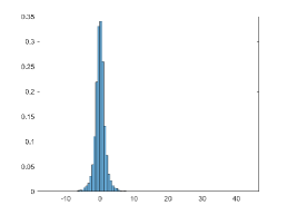
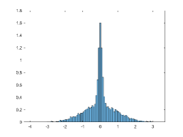
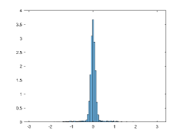
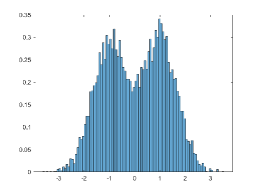
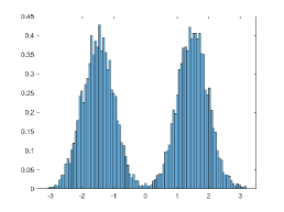
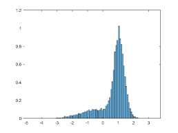
Notes: The panels display histograms of the error distributions used in the data generating processes, M1 to M6. For illustrative purposes these histograms are generated using $10,000$ independent draws and 100 bins (while the DGPs rely on $T=50,100,200$).

Figure 2 illustrates the results of the simulation exercise. For each DGP the individual panels show the trace $R^{2}$ of the multivariate regression of the estimated factors onto the simulated factors for the proposed VBQFA model and the benchmark model developed by CDG. For the heavy-tailed (M1), kurtotic (M2), and outlier distribution (M3) two important observations emerge. While the VBQFA model and the CDG model perform equally well at the median, the VBQFA outperforms the CDG model at the 25^th and 75^th percentile level. Across DGPs the trace $R^{2}$ of the VBQFA model lies between 93.5% and 100% and that of the CDG model between 80.5% and 100% in the tails of the distributions. In addition, while the performance of CDG declines as the number of variables, $N$, increases, the VBQFA model’s performance is robust to changes in the size of the information set. In most cases, the VBQFA’s performance improves in $N$ and $T$ leading to performance gains across growing simulation sizes. The biggest contrast emerges for the bipolar distribution with separated modes, M5. In this case the CDG model outperforms the proposed VBQFA model at all quantile levels and the performance of the VBQFA declines slightly faster in $N$ and $T$ than that of the CDG benchmark. The DGPs M4 and M6 represent in-between cases. Both models perform similarly at the median, but the VBQFA (CDG) model dominates at the $0.75$ ($0.25$) quantile level. In general, both models perform worse on this type of distribution with the trace $R^{2}$ of the VBQFA (CDG) model declining to 68.4% (68.8%) in the least favourable case. The Online Supplement provides detailed tables with the numerical values of the trace $R^{2}$ plotted in Figure 2, as well as comparisons using alternative statistical accuracy metrics.

Figure 2: Trace $R^{2}$

(a) M1

(b) M2

(c) M3

(d) M4

(e) M5

(f) M6

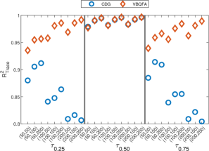
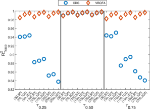
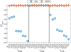
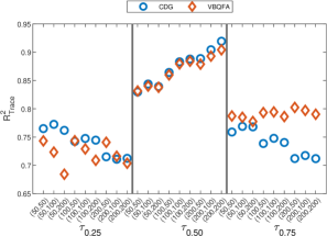
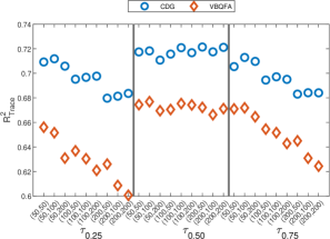
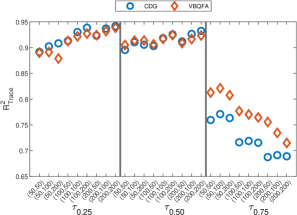
Notes: The different panels depict the trace $R^{2}$ of the multivariate regression of $F$ onto $\hat{F}$ for the CDG, VBQFA, and KS1 quantile factor model for the different data generating processes M1 to M6. The x-axis displays the different Monte Carlo simulation settings, $(N,T)$, for the quantile levels $\tau_{0.25}$, $\tau_{0.50}$, and $\tau_{0.75}$, respectively.

3.2 Quantile factor estimation with dependent idiosyncratic errors

Here we replicate the second Monte Carlo exercise of CDG by adding our proposed estimator of quantile factors. Following these authors we consider the following data generating process

$$x_{it} = \lambda_{1i}f_{1t}+\lambda_{2i}f_{2t}+\left(\lambda_{3i}f_{3t}\right)e_{it},$$ (20)

$$e_{it} = \beta e_{it}+v_{it}+\rho\sum_{j=i-J,j\neq i}^{i+J}v_{jt}$$ (21)

$$f_{jt} = 0.8f_{jt-1}+\epsilon_{jt},j=1,2,$$ (22)

$$f_{3t} = |g_{t}|,$$ (23)

where $\lambda_{1i},\lambda_{2i},\epsilon_{1t},\epsilon_{2t},g_{t}$ are all independent draws from $N(0,1)$ and $\lambda_{3i}\sim U[1,2]$. The autoregressive coefficient $\beta$ captures the serial correlation of $e_{it}$, while the parameters $\rho$ and $J$ capture the cross-sectional correlations of $e_{it}$. As in CDG we have three cases of models that generate our data

1. Independent errors.: $\beta=\rho=0$ and $v_{it}\sim N(0,1)$

2. Independent errors with heavy tails: $\beta=\rho=0$ and $v_{it}\sim t_{3}(0,1)$

3. Serially and cross-sectionally correlated errors: $\beta=0.2$, $\rho=0.4$, $J=3$ and $v_{it}\sim N(0,1)$

This particular DGP is used in order to assess whether autocorrelation in the errors affects quantile factor estimation. We use the exact settings in CDG, namely we generate 1000 artificial datasets for each of M1, M2, M3, for $n,T\in\left\{50,100,200\right\}$, for $\tau\in\left\{0.25,0.50,0.75\right\}$, and we fix $r=3$ in all estimations. Table 1 presents the $R^{2}$s from regressing each of the three true factors to the quantile factor estimates from the output CDG algorithm. That is, this table is equivalent to Table II in the Appendix of CDG. Next Table 2 shows the $R^{2}$s calculated using variational Bayes. Comparing the two tables it is obvious that for the vast majority of cases the two algorithms give identical results. Only for the median estimates of the third factor our algorithm achieves higher $R^{2}$s, however, the overall level of both algorithms is rather low as this third factors enters the DGP in a nonlinear way. Overall, this simulation confirms once more the excellent numerical properties of our algorithm.

Table 1: Simulation Results MCII, CDG, R2

(N,T)	$f_{1}$	$f_{2}$	$f_{3}$	$f_{1}$	$f_{2}$	$f_{3}$	$f_{1}$	$f_{2}$	$f_{3}$
M1	$\tau=0.25$			$\tau=0.50$			$\tau=0.75$
(50,50)	0.959	0.926	0.770	0.967	0.946	0.060	0.957	0.929	0.776
(50,100)	0.965	0.935	0.796	0.972	0.949	0.027	0.965	0.935	0.794
(50,200)	0.967	0.937	0.799	0.974	0.950	0.015	0.967	0.938	0.798
(100,50)	0.979	0.965	0.874	0.984	0.973	0.063	0.979	0.963	0.874
(100,100)	0.983	0.969	0.891	0.986	0.975	0.030	0.983	0.968	0.890
(100,200)	0.984	0.970	0.892	0.987	0.975	0.014	0.984	0.970	0.892
(200,50)	0.989	0.981	0.925	0.992	0.985	0.076	0.989	0.981	0.921
(200,100)	0.992	0.984	0.942	0.993	0.987	0.036	0.992	0.984	0.942
(200,200)	0.992	0.985	0.944	0.994	0.988	0.017	0.992	0.985	0.944
M2	$\tau=0.25$			$\tau=0.50$			$\tau=0.75$
(50,50)	0.923	0.871	0.708	0.957	0.929	0.065	0.927	0.874	0.713
(50,100)	0.942	0.892	0.747	0.962	0.933	0.033	0.941	0.892	0.752
(50,200)	0.946	0.895	0.760	0.966	0.935	0.013	0.945	0.895	0.758
(100,50)	0.964	0.934	0.834	0.979	0.964	0.068	0.965	0.936	0.844
(100,100)	0.974	0.947	0.864	0.983	0.968	0.030	0.973	0.945	0.863
(100,200)	0.974	0.951	0.869	0.984	0.969	0.015	0.975	0.951	0.868
(200,50)	0.982	0.960	0.901	0.989	0.980	0.078	0.982	0.965	0.899
(200,100)	0.987	0.974	0.926	0.992	0.984	0.036	0.987	0.974	0.926
(200,200)	0.988	0.976	0.932	0.992	0.985	0.019	0.988	0.977	0.932
M3	$\tau=0.25$			$\tau=0.50$			$\tau=0.75$
(50,50)	0.948	0.904	0.580	0.960	0.931	0.061	0.946	0.901	0.583
(50,100)	0.957	0.919	0.599	0.965	0.936	0.032	0.957	0.915	0.600
(50,200)	0.960	0.920	0.604	0.967	0.937	0.014	0.960	0.921	0.604
(100,50)	0.975	0.950	0.744	0.980	0.964	0.075	0.974	0.952	0.751
(100,100)	0.979	0.958	0.756	0.983	0.968	0.036	0.979	0.956	0.762
(100,200)	0.980	0.962	0.760	0.984	0.968	0.014	0.980	0.959	0.758
(200,50)	0.986	0.973	0.853	0.989	0.980	0.081	0.985	0.974	0.854
(200,100)	0.989	0.980	0.867	0.991	0.983	0.044	0.990	0.979	0.866
(200,200)	0.990	0.981	0.866	0.992	0.984	0.019	0.990	0.979	0.863

Notes: The table displays the adjusted $R^{2}$ of the regression of the true factor, $F_{i,t}$, onto the estimated factors $\hat{F}_{\cdot,t}$ for the CDG quantile factor model. The rows contain the adjusted $R^{2}$ for the different data generating processes M1 to M3 and Monte Carlo simulation settings $(N,T)$. The columns contain the results for the individual factors at the quantile levels $\tau_{0.25}$, $\tau_{0.50}$, and $\tau_{0.75}$, respectively.

Table 2: Simulation Results MCII, VBQFA, R2

(N,T)	$f_{1}$	$f_{2}$	$f_{3}$	$f_{1}$	$f_{2}$	$f_{3}$	$f_{1}$	$f_{2}$	$f_{3}$
M1	$\tau=0.25$			$\tau=0.50$			$\tau=0.75$
(50,50)	0.954	0.925	0.785	0.961	0.934	0.092	0.946	0.912	0.752
(50,100)	0.963	0.931	0.806	0.968	0.942	0.047	0.960	0.926	0.793
(50,200)	0.966	0.936	0.809	0.972	0.946	0.021	0.965	0.933	0.800
(100,50)	0.980	0.968	0.891	0.984	0.973	0.115	0.979	0.966	0.871
(100,100)	0.984	0.971	0.897	0.987	0.975	0.066	0.983	0.970	0.892
(100,200)	0.985	0.972	0.897	0.988	0.976	0.034	0.985	0.971	0.894
(200,50)	0.991	0.984	0.931	0.993	0.987	0.144	0.990	0.983	0.919
(200,100)	0.992	0.985	0.945	0.993	0.988	0.082	0.992	0.985	0.943
(200,200)	0.993	0.986	0.947	0.994	0.988	0.041	0.993	0.986	0.946
M2	$\tau=0.25$			$\tau=0.50$			$\tau=0.75$
(50,50)	0.921	0.874	0.681	0.946	0.910	0.100	0.910	0.846	0.605
(50,100)	0.938	0.887	0.737	0.956	0.921	0.053	0.931	0.873	0.711
(50,200)	0.945	0.896	0.759	0.964	0.930	0.025	0.940	0.888	0.746
(100,50)	0.963	0.941	0.798	0.979	0.966	0.133	0.959	0.929	0.754
(100,100)	0.976	0.953	0.856	0.983	0.969	0.073	0.973	0.950	0.826
(100,200)	0.977	0.955	0.872	0.985	0.970	0.037	0.976	0.954	0.865
(200,50)	0.984	0.967	0.867	0.991	0.984	0.143	0.980	0.960	0.810
(200,100)	0.988	0.977	0.913	0.992	0.985	0.090	0.987	0.973	0.877
(200,200)	0.989	0.979	0.929	0.993	0.986	0.054	0.989	0.978	0.922
M3	$\tau=0.25$			$\tau=0.50$			$\tau=0.75$
(50,50)	0.944	0.907	0.598	0.948	0.913	0.080	0.935	0.892	0.557
(50,100)	0.952	0.913	0.611	0.956	0.918	0.038	0.949	0.905	0.598
(50,200)	0.957	0.917	0.613	0.960	0.924	0.016	0.955	0.914	0.604
(100,50)	0.976	0.957	0.761	0.980	0.965	0.116	0.974	0.954	0.749
(100,100)	0.979	0.962	0.762	0.982	0.968	0.053	0.978	0.961	0.763
(100,200)	0.981	0.964	0.765	0.984	0.969	0.024	0.981	0.962	0.760
(200,50)	0.988	0.979	0.864	0.990	0.983	0.138	0.987	0.977	0.859
(200,100)	0.990	0.981	0.870	0.992	0.984	0.071	0.990	0.981	0.866
(200,200)	0.991	0.982	0.869	0.992	0.985	0.031	0.990	0.982	0.864

Notes: The table displays the adjusted $R^{2}$ of the regression of the true factor, $F_{i,t}$, onto the estimated factors $\hat{F}_{\cdot,t}$ for the VBQFA quantile factor model. The rows contain the adjusted $R^{2}$ for the different data generating processes M1 to M3 and Monte Carlo simulation settings $(N,T)$. The columns contain the results for the individual factors at the quantile levels $\tau_{0.25}$, $\tau_{0.50}$, and $\tau_{0.75}$, respectively.

3.3 FRED-QD factors

As an additional evidence on the numerical properties of the new algorithm, we extract factors from a large panel of macroeconomic variables for the U.S. In this exercise we use FRED-QD (https://research.stlouisfed.org/econ/mccracken/fred-databases/) that contains 246 macroeconomic and financial indicators observed quarterly for the period 1960Q1 to 2019Q4. Following McCracken and Ng (2020), the raw data are transformed to stationarity and we do not extract factors from series that are high-level aggregates that are related by an identity to subaggregates. This leaves us with a set of 101 subaggregate series to extract factors from. Figure 3 displays the quantile factors extracted with our probabilistic quantile factor model together with the quantile factors extracted using the nonparametric procedure of CDG as well as the conditional mean factors that are extracted using PCA. To simplify representation, we extract quantile factors for three quantile levels, $\tau\in\left\{0.1,0.5,0.9\right\}$, displayed in the columns of the figure and only show the first three factors extracted with each estimation procedure, which are displayed in the rows.

The figure reveals some interesting patters. The first factor of both quantile factor models largely follows the conditional mean factor at the $10\%$ and $50\%$ quantile level. Slight differences emerge at the $90\%$ quantile level. The first quantile factor extracted with the nonparametric procedure of CDG is markedly more volatile and appears to peak more often than both, the first PCA and the first VBQFA quantile factor. Overall, the first factor extracted with our proposed procedure seems to lie between the PCA factor and the CDG quantile factor. Generally, however, both quantile factors move together with the conditional mean factor. This picture changes for the second and third factor. At the $10\%$ quantile level the second VBQFA quantile factor demonstrates more pronounced peaks than the other two procedures throughout the 60s. During the 70s and 80s, however, the factor features three distinct troughs. During the great moderation, all factors broadly move together. This picture is again disrupted during the great depression. The PCA factor drops sharply in 2008Q2 while the two quantile factors show a more muted response. While the PCA quickly recovers to higher levels, especially the VBQFA quantile factor remains at lower or negative level until 2014Q1. At the median, all three factors generally move together, however, the PCA factor again drops more sharply at the onset of the 2008 financial crisis and remains at slightly lower levels thereafter. At the $90\%$ level, the VBQFA quantile factor tends to move together with the PCA factor throughout the first part of the sample, but has more pronounced peaks. During the same period, the CDG quantile factor is less volatile and moves around lower levels. In the second half of the sample up until the financial crisis, both quantile factors tend to move together and seem to lead the cycle of the conditional mean factor. At the onset of the great depression, the PCA factor again drops distinctly while the quantile factors only show a timid response. In the final part of the sample, the VBQFA quantile factor remains at lower levels compared to the other two. For the third factor the CDG quantile factor moves at lower levels during the first part of the sample and moves at higher levels than the other two factors since the great depression at the $10\%$ and $90\%$ level. At the $50\%$ quantile level the behaviour is reversed with the CDG quantile factor being elevated before trending downwards throughout the second half of the sample. In contrast, the VBQFA quantile factor moves together with the PCA factor in the first half of the sample, but is significantly more volatile in the second half at all quantile levels. In addition, during the the financial crisis the third VBQFA quantile factor is characterized by the most pronounced peak an through compared to the other two.

Figure 3: First three quantile factors from FRED-QD.

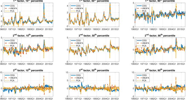
Even though it is hard to draw general conclusions without considering the factor loadings as well, these observations are nonetheless indicative of interesting features. First, quantile factors extracted with either the VBQFA or the CDG approach seem to capture information that is not already contained in the conditional mean factors. This seems to be the case specifically for the tail factors. Second, in line with the previous exercise, both quantile factors also differ from one another with the regularized VBQFA factors being less volatile on average, but peaking more pronouncedly during specific sample periods.

4 Uncertain uncertainty shocks

In this Section we use the quantile factor methodology to extract novel indicators of economic policy uncertainty (EPU). We build on Baker et al. (2016) who construct a single index of economic policy uncertainty for the US, based on textual analysis of millions of newspaper articles. As is the case with most methodologies for constructing uncertainty indices, such measures of uncertainty capture average effects of the underlying concept. On average, high uncertainty has been connected with numerous adverse effects to the economy, that can also be long-lasting, see for example the analysis in Jurado et al. (2015). However, historically there are numerous economic, financial and political events that increase average uncertainty abruptly but do not materialize into widespread recessions or other contractions of the economy. For that reason, various authors suggest that there are two faces of uncertainty that can have diverse outcomes to macroeconomic aggregates. Berger et al. (2020), Caldara et al. (2016), Gambetti et al. (2022) and Segal et al. (2015) are few of many recent empirical studies that document an asymmetric effect of uncertainty shocks depending on the modeling assumptions.

We build on these ideas and we utilize the quantile factor model methodology to measure “low”, “medium”, and “high” uncertainty based on identifying quantiles of the EPU index of Baker et al. (2016). We use data on nine disaggregated categories that are category-specific versions of the aggregate EPU index, namely uncertainties around: monetary policy, fiscal policy, government spending, health care, national security, entitlement programs, regulation, trade policy, and sovereign debt & currency crises. Baker et al. (2016) construct these categorical EPU indices by adding additional search terms to their definition of aggregate EPU. As such, aggregate EPU could also be interpreted as a weighted average of the categorical indices with time-varying weights. In their empirical exercise Baker et al. (2016) find that individual economic sectors are especially attentive to their respective measures of economic policy uncertainty, suggesting that these might capture relevant cross-sector heterogeneity. This provides additional motivation for considering the entire distribution of categorical EPUs. We collect monthly observations on these nine indices as well as the aggregate EPU index for the period 1985M1-2022M10. We estimate a probabilistic quantile factor at three levels, $\tau=0.1,0.5$ and $0.9$, and we do the same for the nonparametric quantile factor using the methodology of CDG. For reference, we also estimate a simple principal component from the nine series. In all three methods, the original data are standardized to have zero mean and variance one, but no other transformation is applied to them as the series are used in their observed levels, without removing outliers or doing further numerical adjustments.

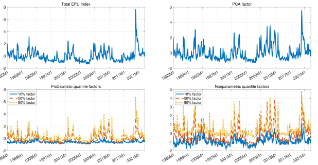
Figure 4 has four panels that allow visual comparison of different estimates of economic policy uncertainty. The top left panel shows the total EPU index of Baker et al. (2016) which (for comparability) has also been standardized to have zero mean and variance one. The top right panel shows the simple PCA estimate from the nine disaggregated categorical EPU series. The aggregate EPU and the PCA index are broadly similar, however, the PCA estimate has more pronounced peaks. Next, the bottom left panel shows the $10\%$, $50\%$ and $90\%$ levels of the VBQFA quantile factor, and the bottom right panel shows the three levels of the CDG quantile factor. Here there are more marked differences between the series. Most importantly the $10\%$ VBQFA factor has noticeably less peaks compared to its CDG counterpart, especially during events of high materialized uncertainty such as the 2020 pandemic. The higher-level factors are also different in the way they peak. The $90\%$ VBQFA factor has correctly estimated levels as it shows the 2020 pandemic to have by far the highest uncertainty in-sample. However, this is not true for the CDG $90\%$ factor which, erratically, attains its highest value during the early 90s US recession and Gulf War.

Figure 4: Aggregate EPU Index vs factor estimates using categorical EPU series: principal component (top right panel); probabilistic quantile factor analysis (bottom left panel); loss-based quantile factor analysis (bottom right panel)

Having established that the quantile factor estimates have noticeable differences with each other, as well as the mean factor and total aggregate uncertainty, we proceed to evaluate the informational content of each series. We broadly follow Bloom (2009) and Jurado et al. (2015) and use vector autoregressions (VARs) in order to evaluate the effects of uncertainty to a series of macroeconomic variables. These authors use large VARs with either eight or 11 macroeconomic and financial variables. To keep things simple, replicable, and transparent, our VARs follow the tradition of simple New Keynesian models and include a measure of output (total industrial production), a measure of prices (total consumer price index) and the (pre-zero lower bound era) monetary policy tool (effective federal funds rate). Our macro data are from the Federal Reserve Economic Data (FRED) database and have mnemonics INDPRO, CPIAUSL, and FEDFUNDS. All series are observed at monthly frequency from 1985M1-2022M10. Other than taking growth rates of output and prices (defined as the first difference of logarithms), we don’t apply any other transformation nor we adjust for the large outliers observed during the 2020-21 period.

We explore the informational content of each of the uncertainty measures plotted in Figure 4 by estimating eight VARs using the three macro variables augmented with each of the uncertainty series (original EPU index; PCA factor; quantile factors using CDG; quantile factors using VBQFA), one at a time. In all specifications we use $p=12$ lags and estimate the models with OLS. We produce forecasts for each of the three macro variables for up to $h=24$ months ahead. All forecasts are iterative pseudo-out-of-sample, where we use the last $60\%$ of the observed sample to compute forecast errors (forecast minus the realization). Table 3 shows the average of the squares of these forecast errors, also known as mean squared forecast errors (MSFEs) for all eight specifications. For comparability the forecast errors for each horizon and each model are relative to the forecast errors generated by the VAR with uncertainty measured using total EPU, which explains why the table only has seven columns (the benchmark VAR with total EPU is a column of ones). Relative MSFE values lower than one for any horizon and any of the three forecasted macro variables, imply that the respective uncertainty indicator is more useful (in a predictive/out-of-sample fit sense) than total EPU. For compactness we only present results for all short forecast horizons $h=1-6$ months, as well as the two longer $h=12,24$ horizons.

The table reveals some interesting patterns. For industrial production, all uncertainty indexes provide marginal predictability in the short-run. The “mean” factor ($f^{PCA}$) achieves gains up to $4\%$ versus the aggregate EPU. Looking at the quantile factors, it is not surprising that these forecast gains are only replicated by their $90\%$ factors, while the $10\%$ and $50\%$ factors are on par with total EPU. This observation implies that quantile factors capture periods of high uncertainty (typically associated with recessions) much better than an average index, translating to higher forecast performance gains. It is noticeable that the highest gains, up to almost $7\%$, are achieved by the VBQFA $90\%$ factor. Moving to CPI, the PCA estimate as well as the vast majority of the uncertainty indexes give forecasting results equal to, or worse than, the VAR using the total EPU index. There are only some small gains when using the $10\%$ quantile factors, namely $f^{CDG}_{0.1}$ and $f^{VBQFA}_{0.1}$. Interestingly, the quantile factors seem to affect the interest rate - which is the conventional monetary policy tool - the most. In particular, $f^{PCA}$ as well as the median and $90\%$ factors (both VBQFA and CDG) seem to improve over total EPU by a large margin, but the highest gains are observed when looking at $10\%$ quantile factors. This result suggests that, on average, low uncertainty events affect the Fed’s decisions more so than high uncertainty. Again, the largest forecasting gains are consistently observed by our VBQFA quantile factor, despite the fact that the CDG quantile factor also performs very well.

Table 3: Relative mean squared forecast errors in the VAR

	rMSFEs of Industrial Production									rMSFEs of CPI Inflation									rMSFEs of Federal Funds Rate
	$f^{PCA}$	$f^{CDG}_{0.1}$	$f^{CDG}_{0.5}$	$f^{CDG}_{0.9}$	$f^{VBQFA}_{0.1}$	$f^{VBQFA}_{0.5}$	$f^{VBQFA}_{0.9}$			$f^{PCA}$	$f^{CDG}_{0.1}$	$f^{CDG}_{0.5}$	$f^{CDG}_{0.9}$	$f^{VBQFA}_{0.1}$	$f^{VBQFA}_{0.5}$	$f^{VBQFA}_{0.9}$			$f^{PCA}$	$f^{CDG}_{0.1}$	$f^{CDG}_{0.5}$	$f^{CDG}_{0.9}$	$f^{VBQFA}_{0.1}$	$f^{VBQFA}_{0.5}$	$f^{VBQFA}_{0.9}$
$h=1$	0.965	0.996	0.981	0.978	0.993	0.988	0.953			1.001	0.972	1.006	1.014	0.982	0.996	1.024			0.921	0.891	0.919	0.939	0.871	0.939	0.935
$h=2$	0.980	0.998	1.005	0.990	0.994	1.012	0.933			1.000	0.971	0.989	1.025	0.965	0.990	1.033			0.925	0.874	0.929	0.934	0.862	0.952	0.971
$h=3$	0.961	0.971	0.970	0.968	0.960	0.974	0.952			1.012	0.994	1.008	1.053	0.992	1.004	1.037			0.937	0.883	0.946	0.936	0.868	0.977	1.001
$h=4$	0.975	1.008	0.992	0.965	1.006	0.982	0.958			1.016	1.005	1.009	1.061	1.022	1.002	1.035			0.940	0.874	0.949	0.925	0.857	0.982	1.004
$h=5$	1.012	1.038	1.028	1.000	1.052	1.017	0.975			1.016	1.002	1.009	1.048	1.019	0.994	1.030			0.947	0.882	0.958	0.921	0.863	0.984	1.006
$h=6$	0.999	1.024	1.006	0.994	1.028	1.008	0.976			1.016	1.014	1.009	1.059	1.028	0.993	1.031			0.962	0.899	0.975	0.926	0.882	0.999	1.017
$h=12$	1.008	1.026	1.019	0.999	1.021	1.006	0.992			1.003	1.021	1.009	1.000	1.028	1.000	0.982			1.002	0.979	1.013	0.950	0.925	1.013	1.029
$h=24$	1.013	1.004	1.019	1.006	1.011	1.014	1.013			1.014	0.999	1.021	1.012	0.987	1.010	1.010			1.010	1.078	1.036	0.958	0.983	1.011	1.017

Notes: The table displays the root mean squared forecast errors (rMSFE) for the PCA, the qPCA, and the VBQFA model for industrial production, CPI inflation, and the Federal Funds rate and forecast horizons 1 to 6, 12, and 24.

Having established that the quantile factor estimated using our methodology has relevant information for macroeconomic aggregates, we proceed into an evaluation of the structural content of the low, medium, and high uncertainty factors. Again, we estimate VAR(12) models using the three macro variables and our three probabilistic quantile factors plus total EPU, but do so by means of the bootstrap estimator of Kilian (1998). We estimate generalized impulse responses of industrial production to a shock in uncertainty in each of the four VAR models. Figure 5 plots the cumulative sum of these responses of industrial production at the 72 month horizon. In the VAR where uncertainty is measured using EPU, shocks to IP are clearly contractionary. However, when considering in turn each of the low, medium and high uncertainty measures that correspond to the $10\%$, $50\%$ and $90\%$ factors, we see that low uncertainty is in fact not recessionary.

Figure 5: Impulse responses of industrial production to total EPU, and quantile factor uncertainty shocks.

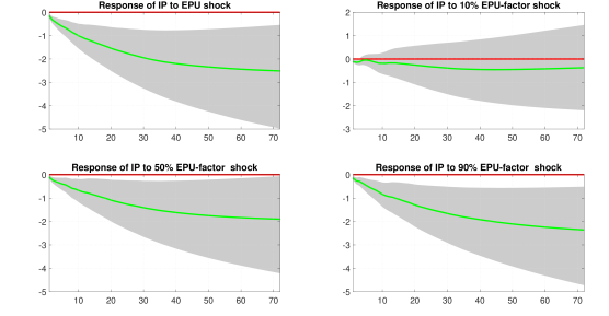
This empirical result complies with empirical observations in recent papers working with various measures and empirical models involving uncertainty. Caldara et al. (2016) show that the negative impact of uncertainty shocks is amplified when financial conditions worsen. When measuring the effects of monetary policy to the economy, Aastveit et al. (2017) document that a monetary policy shock’s effect to output are dampened during periods of high uncertainty. More recently, Berger et al. (2020) measure shocks to realized volatility and identify uncertainty shocks as a by-product using a VAR identification scheme borrowed from the business cycles news literature. Using their identification they find that contemporaneous realized volatility shocks are contractionary while shocks that correspond to uncertainty about the future are not. They attribute this effect to the fact that historically investors hedge realized volatility risk but not implied volatility. Finally, Gambetti et al. (2022) also show that uncertainty shocks can be benign during periods of high disagreement among consumers, while it has the usual contractionary effect to output during periods of high agreement. As in these papers, here we record the empirical result that “low-quantile uncertainty” may not be recessionary, while only “high uncertainty” is correlated with negative response of output. Attempting to pin down the exact channel by which only some manifestations of uncertainty are correlated with, or even cause recessions, is a very useful exercise that is beyond the scope of this paper.

5 Conclusion

We adopt probabilistic inference in the linear quantile factor analysis model. The model allows to capture complex data distributions by modeling each percentile of that distribution using a separate factor analysis model. We allow for penalization of loadings of each quantile factor by adopting a hierarchical shrinkage prior. We propose a computational fast variational Bayes algorithm that we also demonstrate using many synthetic and real data examples, to be numerically accurate. The empirical illustration of measuring uncertainty shows the potential benefits of extracting latent indices using quantile factor analysis, as our estimates outperform traditional averages and PCA in providing accurate early warning signals for industrial production and the interest rate.

Appendix A Variational Bayes inference in the quantile factor model

A.1 Linear quantile factor analysis

The linear quantile factor model is of the form

$$x_{it}=\bm{\lambda}_{i,(\tau)}^{\prime}\bm{f}_{t,(\tau)}+u_{it,(\tau)},\text{ \ \ }u_{it,(\tau)}\sim AL\left(0,\sigma_{i,(\tau)},\tau\right),$$ (A.1)

where $AL(m,\sigma,\tau)$ denotes the univariate asymmetric Laplace density with location parameter $m$, scale parameter $\sigma$, and asymmetry parameter $\tau$. This distribution is of the form

$$u_{it,(\tau)}\sim\frac{\tau(1-\tau)}{\sigma_{i,(\tau)}}\left[e^{(1-\tau)\frac{u_{it,(\tau)}}{\sigma_{i,(\tau)}}}\mathbb{I}(u_{it,(\tau)}\leq 0)+e^{-\tau\frac{u_{it,(\tau)}}{\sigma_{i,(\tau)}}}\mathbb{I}(u_{it,(\tau)}>0)\right].$$ (A.2)

The first step towards Bayesian inference is to rewrite the asymmetric Laplace likelihood as conditionally Gaussian likelihood, because the latter greatly simplifies inference. Following Yu and Moyeed (2001) the AL disturbance term can be written as a normal-exponential mixture of the form

$$u_{it,(\tau)}|z_{it,(\tau)}\ \sim\frac{1}{\sqrt{2\pi z_{it,(\tau)}\sigma_{i,(\tau)}\kappa_{2,(\tau)}^{2}}}\exp\left\{-\frac{\left(x_{it}-\bm{\lambda}_{i,(\tau)}\bm{f}_{(\tau)}-\kappa_{1,(\tau)}z_{it,(\tau)}\right)^{2}}{2z_{it,(\tau)}\sigma_{i,(\tau)}\kappa_{2,(\tau)}^{2}}\right\}\exp\left\{-\frac{z_{it,(\tau)}}{\sigma_{i,(\tau)}}\right\},$$ (A.3)

or more compactly $u_{it}|z_{it}\sim N(\kappa_{1,(\tau)}z_{it,(\tau)},\kappa_{2,(\tau)}^{2}\sigma_{i,(\tau)}z_{it,(\tau)})$, $z_{it,(\tau)}\sim Exp(\sigma_{i,(\tau)})$, where $Exp(\bullet)$ denotes the exponential distribution, $\kappa_{1,(\tau)}=\frac{1-2\tau}{\tau(1-\tau)}$ and $\kappa_{2,(\tau)}^{2}=\frac{2}{\tau(1-\tau)}$. This scale mixture of normals representation gives rise to the following Bayesian quantile factor model

$$x_{it}=\bm{\lambda}_{i,(\tau)}^{\prime}\bm{f}_{t,(\tau)}+\kappa_{1,(\tau)}z_{it,(\tau)}+\kappa_{2,(\tau)}\sqrt{\sigma_{i,(\tau)}z_{it,(\tau)}}u_{it},$$ (A.4)

which is easier to work with because now $v_{it}\sim N(0,1)$.

The prior for $\sigma_{i,(\tau)}$ is of the form $\sigma_{i,(\tau)}\sim G^{-1}(r_{0},s_{0})$, for the factors we assume $\bm{f}_{(\tau)}\sim\prod_{t=1}^{T}N_{r}\left(\bm{0},\bm{I}\right)$, and by definition $z_{it,(\tau)}\sim Exp(\sigma_{i,(\tau)})$. The model is completed by defining the hierarchical structure implied by the sparse Bayesian learning shrinkage prior for $\lambda_{ij,(\tau)}$ for $i=1,\dots,n$ and $j=1,...,r$, which is given by

$$\lambda_{ij,(\tau)}|\alpha_{ij,(\tau)} \sim N(0,\alpha_{ij,(\tau)}^{-1}),$$ (A.5)

$$\alpha_{ij,(\tau)} \sim G\left(a,b\right)$$ (A.6)

where $a$ and $b$ are a tuning parameters set by the user.

Consequently, based on the model likelihood in equation (A.4) and the equations of the prior, the set of latent parameters is $\bm{\theta}_{(\tau)}=\left(\left\{\bm{\lambda}_{i(\tau)},\bm{\alpha}_{i,(\tau)},\bm{\sigma}_{i,(\tau)}\right\}_{i=1}^{n},\left\{\bm{f}_{t,(\tau)},\bm{z}_{t,(\tau)}\right\}_{t=1}^{T}\right)$. The joint prior is $p(\bm{\theta}_{(\tau)})$, the data density is $p(\mathbf{x}|\bm{\theta}_{(\tau)})$, and the parameter posterior is $p(\bm{\theta}_{(\tau)}|\mathbf{x})$. Variational inference requires the introduction of a family of approximating posterior functions $q(\bm{\theta}_{(\tau)}|\mathbf{x})$, where the optimal density $q^{\star}(\bm{\theta}_{(\tau)}|\mathbf{x})$ is the one that maximizes the evidence lower bound (ELBO) $L$

$$q^{\star}(\bm{\theta}_{(\tau)}|\mathbf{x})=\arg\max L=\arg\max\int_{\bm{\theta}_{(\tau)}\in\bm{\Theta}}q(\bm{\theta}_{(\tau)}|\mathbf{x})\log\left\{\frac{p(\mathbf{x}|\bm{\theta}_{(\tau)})p(\bm{\theta}_{(\tau)})}{q(\bm{\theta}_{(\tau)}|\mathbf{x})}\right\}d\bm{\theta}_{(\tau)},$$ (A.7)

where the lower bound can be written compactly as

$$L=\mathbb{E}_{q(\bm{\theta}_{(\tau)}|\mathbf{x})}\left(\log p(\mathbf{x}|\bm{\theta}_{(\tau)})\right)+\mathbb{E}_{q(\bm{\theta}_{(\tau)}|\mathbf{x})}\left(\log p(\bm{\theta}_{(\tau)})\right)-\mathbb{E}_{q(\bm{\theta}_{(\tau)}|\mathbf{x})}\left(\log q(\bm{\theta}_{(\tau)}|\mathbf{x})\right),$$ (A.8)

for $\mathbb{E}_{q(\bm{\theta}_{(\tau)}|\mathbf{x})}(\bullet)$ being the expectation function w.r.t. the variational posterior.

Using calculus of variations, it can be shown that the maximization above can be approximated iteratively by partitioning the parameter set into $M$ groups; see Blei et al. (2017) for details. Consider the decomposition $q(\bm{\theta}_{(\tau)}|\mathbf{x})=\prod_{j=1}^{M}q(\bm{\theta}_{j,(\tau)}|\mathbf{x})$, then optimization of lower bound function can be achieved by sequentially iterating over the densities

$$q(\bm{\theta}_{j,(\tau)}|\mathbf{x})\propto\exp\mathbb{E}_{q(\bm{\theta}_{(-j),(\tau)}|\mathbf{x})}\left(\log p(\bm{\theta}_{j,(\tau)}|\bm{\theta}_{(-j),(\tau)},\mathbf{x})\right),$$ (A.9)

where $\bm{\theta}_{(-j),(\tau)}$ denotes all elements of $\bm{\theta}_{(\tau)}$, excluding those in the j^th group, $j=1,...,M$. Therefore, the variational posterior can be obtained by calculating the variational expectation of the conditional posterior densities.

A crucial question is how to decide on the partitioning of $\bm{\theta}_{(\tau)}$ into the $M$ groups, as this choice affects the overall performance of variational Bayes procedures (see Ormerod et al., 2017). Following Lim et al. (2020) we assume the following factorization of the variational Bayes posterior density:

$$q(\bm{\theta}_{(\tau)}|\mathbf{x})=\prod_{i=1}^{n}\left[q(\bm{\lambda}_{i,(\tau)}|\mathbf{x})q(\sigma_{i,(\tau)}|\mathbf{x})\prod_{j=1}^{r}q(\alpha_{ij,(\tau)}|\mathbf{x})\prod_{t=1}^{T}q(z_{it,(\tau)}|\mathbf{x})\right]\prod_{t=1}^{T}q(\bm{f}_{t,(\tau)}|\mathbf{x}),$$ (A.10)

which implies partial posterior independence between cerain groups of parameters. With the additional assumption that the parameter priors are (conditionally) independent, the joint prior can be written as

$$p(\bm{\theta}_{(\tau)})=\prod_{i}^{n}p(\bm{\lambda}_{i,(\tau)}|\alpha_{i,(\tau)})p(\bm{\alpha}_{i,(\tau)})p(\bm{z}_{i,(\tau)})p(\bm{\sigma}_{i,(\tau)})p(\bm{f}_{(\tau)}).$$ (A.11)

In order to capitalize on these simplifications we need to insert equations (A.10) and (A.11) into the formula for the variational lower bound $L$ given in equation (A.8). Due to this being a lengthy formula (but otherwise easy to derive as it depends on expectations of logarithms of standard densities) we do not present it here. Instead, we focus on deriving expressions for the densities $q(\bm{\theta}_{j,q}|\mathbf{x})$, one at a time for each $j=1,...,M$.

1. Update $\bm{\lambda}_{i,(\tau)}$ for $i=1,....,n$ from

   $$q(\bm{\lambda}_{i,(\tau)}|\mathbf{x})=N_{r}(\bm{\mu}^{\lambda}_{i,(\tau)},\bm{\Sigma}^{\lambda}_{i,(\tau)}),$$ (A.12)

   where $\bm{\Sigma}^{\lambda}_{i,(\tau)}=\left(\frac{1}{\kappa_{2,(\tau)}^{2}}\sum_{t=1}^{T}\mathbb{E}\left(\bm{f}_{t,(\tau)}\right)\mathbb{E}\left(\bm{f}_{t,(\tau)}\right)^{\prime}\mathbb{E}\left(\frac{1}{z_{it,(\tau)}}\right)\mathbb{E}\left(\frac{1}{\sigma_{i,(\tau)}}\right)+\bm{\alpha}_{i,(\tau)}^{-1}\right)^{-1}$ and

   $$\begin{split}\bm{\mu}^{\lambda}_{i,(\tau)}=\bm{\Sigma}^{\lambda}_{i,(\tau)}\left(\frac{1}{\kappa_{2,(\tau)}^{2}}\sum_{t=1}^{T}\mathbb{E}\left(\bm{f}_{t,(\tau)}\right)x_{it}\mathbb{E}\left(\frac{1}{z_{it,(\tau)}}\right)\mathbb{E}\left(\frac{1}{\sigma_{i,(\tau)}}\right)\right.-\\ \left.\frac{\kappa_{1,(\tau)}}{\kappa_{2,(\tau)}^{2}}\mathbb{E}\left(\frac{1}{\sigma_{i,(\tau)}}\right)\sum_{t=1}^{T}\mathbb{E}\left(\bm{f}_{t,(\tau)}\right)\right).\end{split}$$

2. Update $\bm{\alpha}_{i,(\tau)}$ for $i=1,....,n$ from

   $$q(\bm{\alpha}_{i,(\tau)}|\mathbf{x})=G^{-1}\left(a^{\alpha}_{(\tau)},b^{\alpha}_{i,(\tau)}\right),$$ (A.13)

   where $a^{\alpha}_{(\tau)}=a+\frac{1}{2}$ and $b^{\alpha}_{i,(\tau)}=b+\frac{1}{2}\mathbb{E}\left(\lambda_{i,(\tau)}^{2}\right)$.

3. Update $z_{it,(\tau)}$ for $i=1,...,n$ and for $t=1,...,T$ from

   $$q(z_{it,(\tau)}|\mathbf{x})=IG\left(\frac{1}{2},a_{it,(\tau)},b_{it,(\tau)}\right).$$ (A.14)

   where $a_{it,(\tau)}=\mathbb{E}\left(\frac{1}{\sigma_{i,(\tau)}}\right)\left(2+\frac{\kappa_{1,(\tau)}^{2}}{\kappa_{2,(\tau)}^{2}}\right)$ and $b_{it,(\tau)}=\mathbb{E}\left(\frac{1}{\sigma_{i,(\tau)}}\right)\frac{\left(\mathbf{x}_{it}-\mathbb{E}\left(\bm{\lambda}_{i,(\tau)}\right)E\left(\bm{f}_{t,(\tau)}\right)\right)^{2}+\mathbb{E}\left(f_{t,(\tau)}\right)\bm{\Sigma}^{\lambda}_{i,(\tau)}\mathbb{E}\left(f_{t,(\tau)}\right)^{\prime}}{\kappa_{2,(\tau)}^{2}}$. Here $IG(\bullet)$ is the three parameter Inverse Gaussian distribution.

4. Update $\sigma_{i,(\tau)}$ for $i=1,...,n$ from

   $$q(\sigma_{i,(\tau)}|\mathbf{x})=G^{-1}(r_{(\tau)},s_{i,(\tau)}),$$ (A.15)

   where $r_{(\tau)}=r_{0}+3T$ and

   $$s_{i,(\tau)} =s_{0}+\sum_{t=1}^{T}\Biggr{[}\mathbb{E}\left(\frac{1}{z_{it,(\tau)}}\right)\frac{\left(\left(\mathbf{x}_{it}-\mathbb{E}\left(\bm{\lambda}_{i,(\tau)}\right)\mathbb{E}\left(\bm{f}_{t,(\tau)}\right)\right)^{2}+\mathbb{E}\left(\bm{f}_{t,(\tau)}\right)\bm{\Sigma}^{\lambda}_{i,(\tau)}\mathbb{E}\left(\bm{f}_{t,(\tau)}\right)^{\prime}\right)}{2\kappa_{2,(\tau)}^{2}}$$

   $$-\kappa_{1,(\tau)}\frac{X_{it}-\mathbb{E}\left(\bm{\lambda}_{i,(\tau)}\right)\mathbb{E}\left(\bm{f}_{t,(\tau)}\right)}{\kappa_{2,(\tau)}^{2}}+\left(1+\frac{\kappa_{1,(\tau)}^{2}}{2\kappa_{2,(\tau)}^{2}}\right)\mathbb{E}\left(z_{it,(\tau)}\right)\vphantom{\int_{1}^{2}}\Biggr{]}$$

5. Update $\bm{f}_{t,(\tau)}$ for $t=1,....,T$ from

   $$q(\bm{f}_{t,(\tau)}|\mathbf{x})=N_{r}(\bm{\mu}^{f}_{t,(\tau)},\bm{\Sigma}^{f}_{t,(\tau)}),$$ (A.16)

   where $\bm{\Sigma}^{f}_{t,(\tau)}=\left(\frac{1}{\kappa_{2,(\tau)}^{2}}\sum_{i=1}^{n}\mathbb{E}\left(\bm{\lambda}_{i,(\tau)}\right)\mathbb{E}\left(\bm{\lambda}_{i,(\tau)}\right)^{\prime}\mathbb{E}\left(\frac{1}{\bm{z}_{it,(\tau)}}\right)\mathbb{E}\left(\frac{1}{\sigma_{i,(\tau)}}\right)+\bm{I}_{r}\right)^{-1}$ and

   $$\begin{split}\bm{\mu}^{f}_{t,(\tau)}=\bm{\Sigma}^{f}_{t,(\tau)}\left(\frac{1}{\kappa_{2,(\tau)}^{2}}\sum_{i=1}^{n}\mathbb{E}\left(\bm{\lambda}_{i,(\tau)}\right)x_{it}\mathbb{E}\left(\frac{1}{z_{it,(\tau)}}\right)\mathbb{E}\left(\frac{1}{\sigma_{i,(\tau)}}\right)-\right.\\ \left.\frac{\kappa_{1,(\tau)}}{\kappa_{2,(\tau)}^{2}}\sum_{i=1}^{n}\mathbb{E}\left(\frac{1}{\sigma_{i,(\tau)}}\right)\mathbb{E}\left(\bm{\lambda}_{i,(\tau)}\right)\right).\end{split}$$

Also notice that the expectations of each parameter w.r.t. to the variational posterior are defined as:

• $\mathbb{E}(\bm{\lambda}_{i,(\tau)})=\bm{\mu}^{\lambda}_{i,(\tau)}$,

• $\mathbb{E}(\bm{\lambda}_{i,(\tau)}^{2})=\left(\bm{\mu}^{\lambda}_{i,(\tau)}\right)^{2}+diag\left(\bm{\Sigma}_{i,(\tau)}^{\lambda}\right)$,

• $\mathbb{E}(\bm{f}_{t,(\tau)})=\bm{\mu}^{f}_{t,(\tau)}$,

• $\mathbb{E}(\bm{f}_{t,(\tau)}^{2})=\left(\bm{\mu}^{f}_{t,(\tau)}\right)^{2}+diag\left(\bm{\Sigma}_{t,(\tau)}^{f}\right)$,

• $\bm{\alpha}_{i,(\tau)}^{-1}=diag\left(\mathbb{E}\left(\frac{1}{\alpha_{i1,(\tau)}}\right),...,\mathbb{E}\left(\frac{1}{\alpha_{ik,(\tau)}}\right)\right)$,

• $\mathbb{E}\left(\frac{1}{\alpha_{ij,(\tau)}}\right)=\frac{a^{\alpha}_{(\tau)}}{b^{\alpha}_{i,(\tau)}}$

• $\mathbb{E}\left(\frac{1}{\sigma_{i,(\tau)}}\right)=\frac{r_{(\tau)}}{s_{i,(\tau)}}$,

• $\mathbb{E}\left(z_{it}\right)=\frac{\sqrt{b_{it,(\tau)}}K_{3/2}\left(\sqrt{a_{it,(\tau)}b_{it,(\tau)}}\right)}{\sqrt{a_{it,(\tau)}}K_{1/2}\left(\sqrt{a_{it,(\tau)}b_{it,(\tau)}}\right)}$,

• $\mathbb{E}\left(\frac{1}{z_{it}}\right)=\frac{\sqrt{a_{it,(\tau)}}K_{3/2}\left(\sqrt{a_{it,(\tau)}b_{it,(\tau)}}\right)}{\sqrt{b_{it,(\tau)}}K_{1/2}\left(\sqrt{a_{it,(\tau)}b_{it,(\tau)}}\right)}-\frac{1}{b_{it,(\tau)}}$ and $K_{p}(\bullet)$ is the Bessel function of order $p$.

It is evident from the formulas above that each parameter is dependent on the variational expectation of other parameters, such that update of all parameters cannot be achieved in one step. However, parameter updates can be achieved sequentially, similar to the EM-algorithm that is used to maximize likelihood functions.

A.2 Convergence of ELBO and factor selection

Iterating through steps 1-5 maximizes the evidence lower bound $L$. As with all iterative algorithms, it is important to ask whether there are convergence guarantees, whether a global maximum of the ELBO can be achieved, and how many iterations a typical run would require. Blei et al. (2017), who provide an excellent introduction to these issues in general settings, note that different initialization of parameters will lead to slightly different paths of the ELBO. Therefore, as is the case with all EM-type algorithms, achieving a global optimum is not always guaranteed. Additionally, in many cases the ELBO might not converge to a fixed point, despite the fact that parameter updates from one iteration to the next are minimal. Therefore, it is important to choose good initial conditions. For the quantile factor model we initialize the factors to their PCA estimate, such that in step 1 of the algorithm we have during the first iteration $\mathbb{E}\left(\bm{f}_{t,(\tau)}\right)=\widehat{\bm{f}}_{t}^{pca}$. All other parameters are initialized to default values, i.e. they are either vectors of zeros or ones (for mean estimates) or set to $10\bm{I}$ (for variances/covariances).

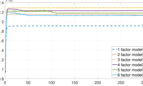
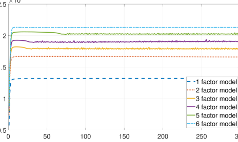
As the ELBO is, by definition, a lower bound to the log-marginal likelihood, its value can be used for model selection. Therefore, it would be interesting to find out not only how quickly the ELBO convergences, but also whether it is a reliable measure for model selection. For that reason we set up a small experiment and generate artificial data from a three-factor model ($r=3$) with Student-t errors, using $T=100$ and $n=50$. We then proceed to estimate quantile factor models with one, two, three, four, five and six factors, respectively.

Figure A.1 shows the estimates of the ELBO over 300 iterations for all six quantile factor models fitted to the artificial data. In all cases, after only a handful of iterations the ELBO convergences towards a fixed value. However, when overfitting the model with four, five and six factors (solid lines) the ELBO does small fluctuations around a fixed value. If we assume a fairly standard convergence criterion (e.g. that the tolerance between two consecutive iterations is 0.0001), then in this three cases the algorithm won’t convergence and it will have to terminate by reaching the maximum number of allowed iterations (300 in the example of Figure A.1). In contrast, when estimating the models with one, two and three factors, convergence is very fast and smooth.

Most importantly, we observe the the estimated model with three factors achieves the highest value of the ELBO. We repeat this experiment, but now we assume in the DGP that the true number of factors is $r=6$. Figure A.2 shows that now the estimated model with six factors is the best. We have also done various simulations for different $T,n,r$ values, and we found that the ELBO selects the correct number of factors in 98-100% of the cases. However, we don’t report these results, as we consider factor selection using the ELBO not a particularly important issue. This is because researchers many times face a fixed number of factors, for example, as it was the case in our empirical exercise with the single uncertainty index, or when using factors for structural analysis. Even when interested in forecasting a variable $y$, in-sample fit measures for choosing factors are less important for two reasons. First, factor estimates are extracted from data $\bm{x}$ without reference to the target variable $y$. Second, measures of out-of-sample performance (e.g. mean squared forecast errors) are always more appropriate when forecasting compared to in-sample measures.

Figure A.1: ELBO estimates when the true number of factors in the DGP is $r=3$

Figure A.2: ELBO estimates when the true number of factors in the DGP is $r=6$

Appendix B Detailed simulation results

Tables B.1 and B.2 present the numerical values of the trace $R^{2}$ statistics used to produced the summary figure in the main document. Tables B.3 and B.4 show the $R^{2}$’s per factor, the exact way this measure is defined in Chen et al. (2021). Finally, tables B.5 and B.6 present the mean squared deviations, which are simply the average squared deviation between each factor estimate and the true value of the factor. The detailed results confirm the summary picture drawn in the main paper, that is, the probabilistic and loss-based estimators have identical performance in the median, but in the tails the former is performing better in the vast majority of cases.

Table B.1: Simulation Results VBQFA; Trace R2

$N=$ $50$ $100$ $200$ $T=$ 50 100 200 50 100 200 50 100 200 $\tau_{0.25}$ 0.935 0.955 0.957 0.958 0.981 0.986 0.969 0.986 0.992 M1 $\tau_{0.50}$ 0.977 0.990 0.995 0.981 0.992 0.996 0.984 0.993 0.997 $\tau_{0.75}$ 0.939 0.959 0.966 0.956 0.976 0.984 0.962 0.981 0.989 $\tau_{0.25}$ 0.985 0.992 0.995 0.987 0.994 0.997 0.988 0.995 0.998 M2 $\tau_{0.50}$ 0.989 0.996 0.998 0.991 0.996 0.998 0.991 0.996 0.998 $\tau_{0.75}$ 0.982 0.991 0.995 0.985 0.993 0.996 0.985 0.993 0.997 $\tau_{0.25}$ 0.998 0.999 1.000 0.998 0.999 1.000 0.998 0.999 1.000 M3 $\tau_{0.50}$ 0.998 0.999 1.000 0.998 0.999 1.000 0.999 0.999 1.000 $\tau_{0.75}$ 0.997 0.999 0.999 0.998 0.999 0.999 0.998 0.999 0.999 $\tau_{0.25}$ 0.743 0.723 0.684 0.744 0.729 0.709 0.741 0.716 0.704 M4 $\tau_{0.50}$ 0.831 0.840 0.838 0.860 0.879 0.884 0.879 0.893 0.904 $\tau_{0.75}$ 0.787 0.785 0.777 0.793 0.794 0.786 0.802 0.797 0.790 $\tau_{0.25}$ 0.656 0.652 0.631 0.637 0.630 0.621 0.626 0.609 0.601 M5 $\tau_{0.50}$ 0.674 0.677 0.670 0.671 0.675 0.674 0.672 0.666 0.671 $\tau_{0.75}$ 0.671 0.672 0.665 0.655 0.652 0.643 0.645 0.631 0.624 $\tau_{0.25}$ 0.890 0.891 0.879 0.913 0.922 0.927 0.924 0.932 0.938 M6 $\tau_{0.50}$ 0.905 0.913 0.914 0.906 0.917 0.924 0.909 0.916 0.923 $\tau_{0.75}$ 0.813 0.821 0.808 0.777 0.770 0.764 0.756 0.735 0.715 Notes: The table displays the trace $R^{2}$ of the multivariate regression of $F$ onto $\hat{F}$ for the VBQFA quantile factor model. The rows contain the trace $R^{2}$ for the different data generating processes M1 to M6 and for the quantile levels $\tau_{0.25}$, $\tau_{0.50}$, and $\tau_{0.75}$, respectively. The columns contain the different Monte Carlo simulation settings for $N$ and $T$. The trace $R^{2}$ is given by $R^{2}_{\hat{F},F}=\hat{E}tr(\hat{F}^{\prime}P_{F}\hat{F})/\hat{E}tr(\hat{F}^{\prime}\hat{F})$, where $P_{F}=F(F^{\prime}F)^{-1}F^{\prime}$.

Table B.2: Simulation Results CDG; Trace R2

$N=$ $50$ $100$ $200$ $T=$ 50 100 200 50 100 200 50 100 200 $\tau_{0.25}$ 0.880 0.905 0.912 0.841 0.848 0.864 0.809 0.816 0.807 M1 $\tau_{0.50}$ 0.979 0.990 0.995 0.982 0.992 0.996 0.983 0.992 0.996 $\tau_{0.75}$ 0.885 0.914 0.909 0.839 0.855 0.855 0.809 0.822 0.805 $\tau_{0.25}$ 0.941 0.941 0.944 0.883 0.886 0.890 0.852 0.855 0.838 M2 $\tau_{0.50}$ 0.990 0.995 0.997 0.991 0.996 0.998 0.991 0.996 0.998 $\tau_{0.75}$ 0.944 0.942 0.950 0.875 0.890 0.895 0.862 0.848 0.841 $\tau_{0.25}$ 0.944 0.949 0.951 0.890 0.889 0.888 0.869 0.867 0.848 M3 $\tau_{0.50}$ 0.998 0.999 1.000 0.998 0.999 1.000 0.999 0.999 1.000 $\tau_{0.75}$ 0.959 0.939 0.944 0.895 0.890 0.889 0.871 0.867 0.855 $\tau_{0.25}$ 0.765 0.773 0.762 0.742 0.748 0.745 0.715 0.711 0.712 M4 $\tau_{0.50}$ 0.830 0.844 0.839 0.864 0.883 0.888 0.889 0.904 0.919 $\tau_{0.75}$ 0.759 0.769 0.768 0.739 0.748 0.740 0.712 0.717 0.712 $\tau_{0.25}$ 0.709 0.712 0.706 0.695 0.697 0.698 0.680 0.681 0.684 M5 $\tau_{0.50}$ 0.717 0.718 0.711 0.716 0.721 0.717 0.721 0.718 0.721 $\tau_{0.75}$ 0.705 0.713 0.710 0.695 0.697 0.695 0.683 0.684 0.684 $\tau_{0.25}$ 0.892 0.902 0.908 0.913 0.930 0.939 0.923 0.937 0.942 M6 $\tau_{0.50}$ 0.895 0.910 0.906 0.903 0.918 0.925 0.912 0.926 0.932 $\tau_{0.75}$ 0.759 0.771 0.763 0.716 0.719 0.715 0.688 0.691 0.689 Notes: The table displays the trace $R^{2}$ of the multivariate regression of $F$ onto $\hat{F}$ for the CDG quantile factor model. The rows contain the trace $R^{2}$ for the different data generating processes M1 to M6 and for the quantile levels $\tau_{0.25}$, $\tau_{0.50}$, and $\tau_{0.75}$, respectively. The columns contain the different Monte Carlo simulation settings for $N$ and $T$. The trace $R^{2}$ is given by $R^{2}_{\hat{F},F}=\hat{E}tr(\hat{F}^{\prime}P_{F}\hat{F})/\hat{E}tr(\hat{F}^{\prime}\hat{F})$, where $P_{F}=F(F^{\prime}F)^{-1}F^{\prime}$.

Table B.3: Simulation Results VBQFA; $R^{2}$ per quantile factor

(N,T)	$f_{1}$	$f_{2}$	$f_{3}$	$f_{1}$	$f_{2}$	$f_{3}$	$f_{1}$	$f_{2}$	$f_{3}$		(N,T)	$f_{1}$	$f_{2}$	$f_{3}$	$f_{1}$	$f_{2}$	$f_{3}$	$f_{1}$	$f_{2}$	$f_{3}$
M1	$\tau=0.25$			$\tau=0.50$			$\tau=0.75$				M4	$\tau=0.25$			$\tau=0.50$			$\tau=0.75$
(50,50)	0.956	0.956	0.953	0.972	0.972	0.971	0.953	0.954	0.953		(50,50)	0.804	0.788	0.812	0.839	0.834	0.847	0.814	0.810	0.813
(50,100)	0.981	0.982	0.984	0.990	0.989	0.990	0.983	0.980	0.982		(50,100)	0.807	0.802	0.829	0.863	0.853	0.872	0.824	0.814	0.832
(50,200)	0.991	0.992	0.991	0.995	0.995	0.995	0.991	0.992	0.991		(50,200)	0.816	0.810	0.806	0.870	0.871	0.865	0.832	0.830	0.822
(100,50)	0.967	0.969	0.966	0.978	0.979	0.978	0.967	0.967	0.966		(100,50)	0.763	0.795	0.777	0.851	0.856	0.850	0.804	0.811	0.802
(100,100)	0.989	0.988	0.989	0.992	0.991	0.992	0.988	0.988	0.988		(100,100)	0.784	0.780	0.785	0.875	0.878	0.876	0.819	0.814	0.815
(100,200)	0.994	0.995	0.995	0.996	0.996	0.996	0.994	0.995	0.994		(100,200)	0.799	0.788	0.787	0.893	0.886	0.879	0.826	0.822	0.805
(200,50)	0.975	0.973	0.972	0.982	0.982	0.981	0.974	0.974	0.972		(200,50)	0.750	0.765	0.752	0.860	0.873	0.863	0.803	0.814	0.801
(200,100)	0.990	0.990	0.990	0.992	0.992	0.992	0.990	0.990	0.990		(200,100)	0.757	0.748	0.771	0.891	0.880	0.886	0.819	0.799	0.812
(200,200)	0.996	0.996	0.996	0.996	0.996	0.996	0.996	0.996	0.996		(200,200)	0.765	0.745	0.773	0.895	0.899	0.902	0.812	0.802	0.813
M2	$\tau=0.25$			$\tau=0.50$			$\tau=0.75$				M5	$\tau=0.25$			$\tau=0.50$			$\tau=0.75$
(50,50)	0.983	0.983	0.983	0.986	0.986	0.986	0.981	0.981	0.982		(50,50)	0.770	0.749	0.767	0.777	0.753	0.772	0.776	0.749	0.771
(50,100)	0.992	0.992	0.993	0.995	0.994	0.995	0.992	0.992	0.992		(50,100)	0.773	0.754	0.793	0.786	0.766	0.795	0.781	0.763	0.791
(50,200)	0.996	0.996	0.996	0.997	0.997	0.997	0.996	0.996	0.996		(50,200)	0.779	0.771	0.778	0.791	0.785	0.780	0.783	0.787	0.779
(100,50)	0.985	0.986	0.986	0.989	0.989	0.989	0.985	0.985	0.985		(100,50)	0.725	0.744	0.733	0.736	0.754	0.751	0.734	0.748	0.744
(100,100)	0.994	0.994	0.994	0.995	0.995	0.995	0.994	0.994	0.994		(100,100)	0.744	0.740	0.744	0.759	0.755	0.764	0.750	0.751	0.752
(100,200)	0.997	0.997	0.997	0.998	0.998	0.998	0.997	0.997	0.997		(100,200)	0.759	0.746	0.747	0.784	0.758	0.760	0.767	0.753	0.748
(200,50)	0.987	0.987	0.986	0.990	0.991	0.990	0.987	0.987	0.986		(200,50)	0.707	0.734	0.687	0.724	0.745	0.718	0.721	0.740	0.703
(200,100)	0.995	0.995	0.995	0.996	0.996	0.996	0.995	0.995	0.995		(200,100)	0.722	0.700	0.732	0.741	0.726	0.751	0.732	0.712	0.737
(200,200)	0.998	0.998	0.998	0.998	0.998	0.998	0.997	0.997	0.997		(200,200)	0.721	0.706	0.744	0.746	0.731	0.766	0.720	0.719	0.753
M3	$\tau=0.25$			$\tau=0.50$			$\tau=0.75$				M6	$\tau=0.25$			$\tau=0.50$			$\tau=0.75$
(50,50)	0.997	0.997	0.997	0.997	0.998	0.998	0.997	0.997	0.997		(50,50)	0.904	0.902	0.907	0.921	0.910	0.913	0.837	0.832	0.838
(50,100)	0.999	0.999	0.999	0.999	0.999	0.999	0.999	0.999	0.999		(50,100)	0.919	0.908	0.916	0.925	0.919	0.929	0.859	0.834	0.853
(50,200)	0.999	0.999	0.999	0.999	0.999	1.000	0.999	0.999	0.999		(50,200)	0.923	0.916	0.914	0.929	0.926	0.926	0.842	0.843	0.842
(100,50)	0.997	0.997	0.997	0.998	0.998	0.998	0.997	0.997	0.997		(100,50)	0.912	0.916	0.914	0.923	0.924	0.927	0.814	0.805	0.810
(100,100)	0.999	0.999	0.999	0.999	0.999	0.999	0.999	0.999	0.999		(100,100)	0.926	0.926	0.920	0.935	0.932	0.931	0.815	0.799	0.797
(100,200)	1.000	1.000	1.000	1.000	1.000	1.000	0.999	0.999	0.999		(100,200)	0.937	0.930	0.931	0.944	0.938	0.935	0.819	0.797	0.783
(200,50)	0.998	0.998	0.998	0.998	0.998	0.998	0.998	0.998	0.998		(200,50)	0.926	0.925	0.919	0.932	0.937	0.928	0.796	0.798	0.792
(200,100)	0.999	0.999	0.999	0.999	0.999	0.999	0.999	0.999	0.999		(200,100)	0.933	0.927	0.934	0.941	0.934	0.940	0.769	0.757	0.776
(200,200)	1.000	1.000	1.000	1.000	1.000	1.000	1.000	1.000	1.000		(200,200)	0.943	0.939	0.938	0.945	0.945	0.942	0.767	0.725	0.764

Notes: The table displays the adjusted $R^{2}$ of the regression of the true factor, $F_{i,t}$, onto the estimated factors $\hat{F}_{\cdot,t}$ for the VBQFA quantile factor model. The rows contain the adjusted $R^{2}$ for the different data generating processes M1 to M6 and Monte Carlo simulation settings $(N,T)$. The columns contain the results for the individual factors at the quantile levels $\tau_{0.25}$, $\tau_{0.50}$, and $\tau_{0.75}$, respectively.

Table B.4: Simulation Results CDG; $R^{2}$ per quantile factor

(N,T)	$f_{1}$	$f_{2}$	$f_{3}$	$f_{1}$	$f_{2}$	$f_{3}$	$f_{1}$	$f_{2}$	$f_{3}$		(N,T)	$f_{1}$	$f_{2}$	$f_{3}$	$f_{1}$	$f_{2}$	$f_{3}$	$f_{1}$	$f_{2}$	$f_{3}$
M1	$\tau=0.25$			$\tau=0.50$			$\tau=0.75$				M4	$\tau=0.25$			$\tau=0.50$			$\tau=0.75$
(50,50)	0.910	0.907	0.917	0.978	0.978	0.978	0.919	0.910	0.917		(50,50)	0.805	0.785	0.804	0.870	0.849	0.870	0.794	0.789	0.798
(50,100)	0.940	0.927	0.939	0.990	0.989	0.990	0.940	0.940	0.950		(50,100)	0.799	0.807	0.825	0.879	0.875	0.887	0.794	0.793	0.827
(50,200)	0.944	0.950	0.940	0.995	0.995	0.995	0.945	0.941	0.943		(50,200)	0.819	0.805	0.793	0.888	0.880	0.874	0.818	0.813	0.803
(100,50)	0.873	0.866	0.878	0.981	0.982	0.982	0.879	0.859	0.879		(100,50)	0.757	0.779	0.775	0.883	0.883	0.881	0.757	0.761	0.783
(100,100)	0.874	0.883	0.879	0.992	0.991	0.992	0.881	0.888	0.894		(100,100)	0.777	0.778	0.782	0.895	0.901	0.903	0.783	0.777	0.782
(100,200)	0.894	0.889	0.896	0.996	0.996	0.996	0.886	0.872	0.893		(100,200)	0.774	0.778	0.799	0.911	0.907	0.905	0.778	0.776	0.775
(200,50)	0.835	0.836	0.829	0.983	0.984	0.983	0.830	0.831	0.833		(200,50)	0.740	0.752	0.713	0.893	0.900	0.896	0.719	0.748	0.727
(200,100)	0.838	0.830	0.858	0.992	0.992	0.992	0.838	0.839	0.862		(200,100)	0.719	0.736	0.758	0.918	0.904	0.918	0.741	0.734	0.752
(200,200)	0.839	0.825	0.837	0.996	0.996	0.996	0.827	0.821	0.844		(200,200)	0.743	0.730	0.757	0.923	0.928	0.932	0.742	0.739	0.744
M2	$\tau=0.25$			$\tau=0.50$			$\tau=0.75$				M5	$\tau=0.25$			$\tau=0.50$			$\tau=0.75$
(50,50)	0.957	0.950	0.949	0.989	0.989	0.990	0.963	0.948	0.951		(50,50)	0.766	0.748	0.757	0.784	0.765	0.778	0.766	0.760	0.745
(50,100)	0.956	0.950	0.954	0.995	0.995	0.995	0.953	0.957	0.956		(50,100)	0.758	0.755	0.791	0.773	0.773	0.808	0.760	0.752	0.784
(50,200)	0.955	0.958	0.954	0.997	0.997	0.997	0.967	0.958	0.960		(50,200)	0.779	0.765	0.767	0.790	0.787	0.777	0.774	0.777	0.765
(100,50)	0.885	0.899	0.904	0.991	0.991	0.991	0.898	0.876	0.899		(100,50)	0.720	0.735	0.742	0.753	0.758	0.770	0.725	0.732	0.734
(100,100)	0.890	0.901	0.913	0.995	0.995	0.995	0.910	0.901	0.907		(100,100)	0.741	0.732	0.740	0.770	0.770	0.762	0.747	0.733	0.735
(100,200)	0.901	0.899	0.923	0.998	0.998	0.998	0.906	0.898	0.922		(100,200)	0.740	0.745	0.754	0.776	0.766	0.770	0.744	0.739	0.746
(200,50)	0.866	0.857	0.863	0.991	0.991	0.991	0.882	0.870	0.861		(200,50)	0.708	0.717	0.682	0.743	0.751	0.746	0.698	0.711	0.705
(200,100)	0.867	0.862	0.880	0.996	0.996	0.996	0.849	0.861	0.873		(200,100)	0.695	0.707	0.737	0.755	0.737	0.763	0.714	0.700	0.728
(200,200)	0.852	0.855	0.850	0.998	0.998	0.998	0.860	0.846	0.863		(200,200)	0.724	0.699	0.734	0.757	0.746	0.772	0.714	0.711	0.734
M3	$\tau=0.25$			$\tau=0.50$			$\tau=0.75$				M6	$\tau=0.25$			$\tau=0.50$			$\tau=0.75$
(50,50)	0.958	0.945	0.954	0.998	0.998	0.998	0.973	0.953	0.968		(50,50)	0.917	0.905	0.919	0.927	0.925	0.924	0.810	0.791	0.796
(50,100)	0.956	0.958	0.962	0.999	0.999	0.999	0.950	0.952	0.951		(50,100)	0.927	0.924	0.928	0.934	0.935	0.939	0.806	0.797	0.831
(50,200)	0.960	0.962	0.958	1.000	1.000	1.000	0.952	0.950	0.957		(50,200)	0.934	0.933	0.931	0.939	0.937	0.936	0.815	0.809	0.803
(100,50)	0.903	0.897	0.899	0.998	0.998	0.998	0.909	0.901	0.909		(100,50)	0.926	0.929	0.928	0.934	0.934	0.939	0.735	0.757	0.758
(100,100)	0.911	0.894	0.904	0.999	0.999	0.999	0.905	0.909	0.899		(100,100)	0.944	0.944	0.943	0.950	0.945	0.948	0.755	0.740	0.766
(100,200)	0.899	0.881	0.925	1.000	1.000	1.000	0.896	0.896	0.908		(100,200)	0.954	0.950	0.953	0.957	0.957	0.950	0.762	0.754	0.758
(200,50)	0.883	0.870	0.876	0.999	0.999	0.999	0.879	0.880	0.870		(200,50)	0.935	0.938	0.927	0.943	0.945	0.943	0.712	0.722	0.698
(200,100)	0.870	0.862	0.897	0.999	0.999	0.999	0.869	0.868	0.884		(200,100)	0.942	0.952	0.947	0.957	0.954	0.957	0.714	0.709	0.738
(200,200)	0.862	0.861	0.852	1.000	1.000	1.000	0.858	0.867	0.868		(200,200)	0.954	0.949	0.953	0.962	0.961	0.960	0.718	0.698	0.744

Notes: The table displays the adjusted $R^{2}$ of the regression of the true factor, $F_{i,t}$, onto the estimated factors $\hat{F}_{\cdot,t}$ for the CDG quantile factor model. The rows contain the adjusted $R^{2}$ for the different data generating processes M1 to M6 and Monte Carlo simulation settings $(N,T)$. The columns contain the results for the individual factors at the quantile levels $\tau_{0.25}$, $\tau_{0.50}$, and $\tau_{0.75}$, respectively.

Table B.5: Simulation Results VBQFA; MSD per quantile factor

(N,T)	$f_{1}$	$f_{2}$	$f_{3}$	$f_{1}$	$f_{2}$	$f_{3}$	$f_{1}$	$f_{2}$	$f_{3}$		(N,T)	$f_{1}$	$f_{2}$	$f_{3}$	$f_{1}$	$f_{2}$	$f_{3}$	$f_{1}$	$f_{2}$	$f_{3}$
M1	$\tau=0.25$			$\tau=0.50$			$\tau=0.75$				M4	$\tau=0.25$			$\tau=0.50$			$\tau=0.75$
(50,50)	1.931	1.904	1.950	1.929	1.914	1.954	1.927	1.921	1.951		(50,50)	1.930	1.887	1.954	1.919	1.861	1.940	1.916	1.867	1.941
(50,100)	2.000	1.995	2.001	2.003	1.992	2.008	2.004	1.997	2.009		(50,100)	2.020	1.957	1.923	2.017	1.964	1.939	2.017	1.968	1.970
(50,200)	1.955	1.965	2.005	1.959	1.963	2.014	1.957	1.965	2.005		(50,200)	1.923	1.931	1.995	1.923	1.944	2.013	1.925	1.955	2.036
(100,50)	2.055	1.995	1.996	2.055	1.997	1.991	2.056	2.001	1.990		(100,50)	2.018	1.978	1.985	2.010	1.987	2.006	2.005	1.983	2.017
(100,100)	1.945	1.957	2.015	1.949	1.951	2.014	1.949	1.951	2.020		(100,100)	1.942	1.957	2.018	1.953	1.941	2.048	1.953	1.947	2.030
(100,200)	1.905	1.938	1.945	1.901	1.939	1.937	1.902	1.941	1.944		(100,200)	1.916	1.975	1.948	1.908	1.978	1.982	1.908	1.983	1.993
(200,50)	1.935	1.997	2.086	1.934	2.000	2.088	1.936	2.001	2.085		(200,50)	1.895	2.009	2.060	1.889	1.996	2.078	1.889	1.993	2.070
(200,100)	1.953	2.021	1.979	1.952	2.018	1.979	1.956	2.019	1.977		(200,100)	1.990	2.064	1.997	1.991	2.071	1.975	1.987	2.075	1.961
(200,200)	2.020	1.989	1.939	2.022	1.991	1.940	2.019	1.991	1.935		(200,200)	2.041	1.952	2.017	2.042	1.958	1.998	2.048	1.968	2.016
M2	$\tau=0.25$			$\tau=0.50$			$\tau=0.75$				M5	$\tau=0.25$			$\tau=0.50$			$\tau=0.75$
(50,50)	1.929	1.915	1.893	1.927	1.909	1.893	1.928	1.909	1.899		(50,50)	1.988	1.999	2.009	1.992	2.006	2.008	1.987	1.998	2.007
(50,100)	1.976	2.041	1.973	1.979	2.041	1.980	1.980	2.043	1.976		(50,100)	2.008	2.011	1.916	1.994	1.997	1.942	1.998	2.010	1.949
(50,200)	1.971	1.939	1.942	1.973	1.937	1.945	1.973	1.938	1.941		(50,200)	1.967	2.060	1.994	1.980	2.054	2.011	1.993	2.067	2.012
(100,50)	2.039	1.971	1.962	2.039	1.971	1.960	2.038	1.969	1.961		(100,50)	1.983	2.083	2.033	1.960	2.090	2.045	1.963	2.093	2.037
(100,100)	1.956	1.946	2.027	1.956	1.942	2.027	1.956	1.944	2.024		(100,100)	2.019	1.997	2.071	2.038	1.983	2.060	2.040	1.998	2.066
(100,200)	1.897	1.969	1.915	1.895	1.971	1.914	1.895	1.969	1.915		(100,200)	1.976	1.905	2.018	1.977	1.904	2.035	1.981	1.896	2.018
(200,50)	1.932	1.965	2.065	1.934	1.966	2.067	1.934	1.967	2.067		(200,50)	1.925	1.993	2.014	1.920	1.995	2.013	1.921	1.994	2.022
(200,100)	1.962	2.003	1.997	1.962	2.003	1.996	1.962	2.004	1.997		(200,100)	1.981	2.025	1.974	1.985	2.017	1.968	1.970	2.022	1.969
(200,200)	2.024	1.967	1.950	2.025	1.967	1.949	2.024	1.968	1.949		(200,200)	1.995	1.979	2.006	2.003	1.971	2.008	2.009	1.970	2.003
M3	$\tau=0.25$			$\tau=0.50$			$\tau=0.75$				M6	$\tau=0.25$			$\tau=0.50$			$\tau=0.75$
(50,50)	1.922	1.914	1.900	1.919	1.912	1.900	1.922	1.914	1.901		(50,50)	1.941	1.940	1.923	1.937	1.935	1.930	1.936	1.929	1.918
(50,100)	1.989	2.022	1.976	1.988	2.022	1.978	1.988	2.022	1.975		(50,100)	1.982	2.032	1.990	1.980	2.032	1.982	1.980	2.036	1.972
(50,200)	1.929	1.932	1.975	1.929	1.930	1.979	1.930	1.932	1.976		(50,200)	1.943	1.941	1.949	1.936	1.944	1.953	1.935	1.940	1.954
(100,50)	2.046	2.000	1.949	2.046	2.000	1.948	2.046	2.000	1.949		(100,50)	2.029	2.020	1.968	2.023	2.025	1.971	2.022	2.014	1.980
(100,100)	1.954	1.926	2.012	1.953	1.926	2.012	1.954	1.926	2.012		(100,100)	1.972	1.944	2.004	1.968	1.945	2.023	1.961	1.934	2.019
(100,200)	1.884	1.952	1.940	1.883	1.952	1.940	1.884	1.952	1.940		(100,200)	1.914	1.945	1.963	1.917	1.939	1.969	1.921	1.929	1.987
(200,50)	1.929	1.983	2.031	1.929	1.983	2.031	1.929	1.983	2.032		(200,50)	1.913	1.946	2.047	1.917	1.951	2.052	1.910	1.985	1.988
(200,100)	1.961	2.044	1.975	1.961	2.044	1.975	1.961	2.044	1.975		(200,100)	1.973	2.023	2.003	1.977	2.017	2.018	1.967	2.031	2.069
(200,200)	2.019	1.944	1.941	2.019	1.944	1.941	2.019	1.944	1.941		(200,200)	2.011	1.945	1.980	2.009	1.934	1.985	2.004	1.920	1.953

Notes: The table displays the mean squared deviations (MSD) true factor, $F_{i,t}$, and the estimated factors $\hat{F}_{i,t}$ for the VBQFA quantile factor model. The rows contain the MSD for the different data generating processes M1 to M6 and Monte Carlo simulation settings $(N,T)$. The columns contain the results for the individual factors at the quantile levels $\tau_{0.25}$, $\tau_{0.50}$, and $\tau_{0.75}$, respectively.

Table B.6: Simulation Results CDG; MSD per quantile factor

(N,T)	$f_{1}$	$f_{2}$	$f_{3}$	$f_{1}$	$f_{2}$	$f_{3}$	$f_{1}$	$f_{2}$	$f_{3}$		(N,T)	$f_{1}$	$f_{2}$	$f_{3}$	$f_{1}$	$f_{2}$	$f_{3}$	$f_{1}$	$f_{2}$	$f_{3}$
M1	$\tau=0.25$			$\tau=0.50$			$\tau=0.75$				M4	$\tau=0.25$			$\tau=0.50$			$\tau=0.75$
(50,50)	1.865	1.920	1.898	1.855	2.026	1.957	1.910	2.008	2.032		(50,50)	1.917	1.960	1.970	1.889	1.964	1.991	1.924	2.006	2.009
(50,100)	1.904	1.994	1.987	1.905	2.067	1.977	1.962	1.960	1.877		(50,100)	2.003	2.014	1.973	1.870	2.003	1.999	1.916	1.938	1.943
(50,200)	1.925	1.970	1.945	1.991	1.939	1.975	1.982	2.009	1.921		(50,200)	1.978	2.020	1.974	1.933	2.037	1.966	1.896	1.971	1.966
(100,50)	2.073	1.984	1.982	2.103	2.077	1.908	2.051	2.052	1.919		(100,50)	2.070	2.064	1.946	2.060	1.998	1.942	2.072	2.052	2.029
(100,100)	1.960	2.016	2.028	1.959	2.051	1.929	1.947	1.965	2.022		(100,100)	1.973	2.058	1.963	1.956	2.080	1.910	1.936	2.056	2.045
(100,200)	1.878	1.957	1.997	1.961	2.003	1.901	1.964	1.980	1.948		(100,200)	1.991	1.942	2.036	1.897	1.869	1.959	2.009	1.999	1.966
(200,50)	2.026	2.042	1.953	2.008	1.990	1.993	1.956	2.026	1.983		(200,50)	2.085	2.023	1.966	2.075	1.997	2.106	1.974	1.977	1.976
(200,100)	1.959	2.017	2.027	1.963	2.008	2.005	2.000	2.004	2.014		(200,100)	1.979	1.936	2.014	1.908	2.035	2.037	1.912	1.990	1.963
(200,200)	2.001	2.075	1.907	1.998	1.984	2.063	2.007	2.028	2.001		(200,200)	1.974	2.001	1.959	1.963	1.953	1.970	2.049	2.043	1.970
M2	$\tau=0.25$			$\tau=0.50$			$\tau=0.75$				M5	$\tau=0.25$			$\tau=0.50$			$\tau=0.75$
(50,50)	1.932	1.970	1.932	1.933	1.966	1.938	1.977	1.907	1.911		(50,50)	1.954	2.030	1.913	1.899	1.911	1.920	1.919	1.957	1.960
(50,100)	1.950	2.035	1.922	1.929	2.027	1.955	1.949	1.985	2.002		(50,100)	1.978	2.023	1.932	1.949	2.020	1.999	2.020	1.914	1.959
(50,200)	1.921	1.940	1.902	1.980	1.942	1.978	1.915	1.958	1.922		(50,200)	1.962	1.967	2.008	1.978	1.969	1.999	1.929	1.966	1.930
(100,50)	2.133	2.051	1.985	2.115	2.010	1.890	2.119	2.011	1.917		(100,50)	2.069	1.960	1.996	2.027	1.941	2.034	2.078	1.966	1.959
(100,100)	1.961	2.005	1.971	1.962	2.044	1.905	1.954	1.981	1.964		(100,100)	1.954	2.012	1.931	1.951	2.022	1.979	1.929	1.952	2.011
(100,200)	1.912	1.989	1.982	1.898	1.931	1.915	1.968	1.949	1.955		(100,200)	1.991	1.944	2.015	1.957	1.935	2.014	1.979	1.958	1.956
(200,50)	1.950	1.977	2.074	2.047	1.955	2.029	1.978	2.031	1.974		(200,50)	2.111	1.941	2.030	2.040	1.914	1.936	2.032	2.011	1.957
(200,100)	1.962	2.070	1.939	1.946	1.981	1.997	1.940	2.078	1.992		(200,100)	2.001	1.994	1.954	1.996	2.047	2.019	1.945	1.998	1.961
(200,200)	1.973	1.962	1.979	1.964	2.017	2.026	1.990	2.070	2.022		(200,200)	1.989	2.047	1.977	2.031	1.987	1.972	2.089	2.024	2.003
M3	$\tau=0.25$			$\tau=0.50$			$\tau=0.75$				M6	$\tau=0.25$			$\tau=0.50$			$\tau=0.75$
(50,50)	1.899	1.907	1.902	1.934	1.974	1.947	1.893	1.916	1.926		(50,50)	1.926	1.996	1.942	1.970	1.994	1.977	1.972	1.921	1.957
(50,100)	2.001	2.014	1.976	1.941	2.003	1.963	1.940	2.021	1.970		(50,100)	1.918	2.042	2.026	1.950	1.992	1.990	1.986	2.069	1.874
(50,200)	1.866	1.949	1.982	1.884	1.948	1.973	1.904	2.039	1.926		(50,200)	1.943	2.055	1.958	1.979	1.912	1.883	1.925	1.968	1.939
(100,50)	2.119	2.029	1.983	2.088	2.078	1.992	2.138	2.062	1.937		(100,50)	2.079	2.057	2.010	2.143	2.064	1.987	2.105	1.908	1.933
(100,100)	2.007	2.043	1.995	1.980	2.007	1.909	1.988	2.021	1.962		(100,100)	1.968	2.019	1.955	1.937	2.040	1.952	1.950	1.947	2.015
(100,200)	1.875	2.025	2.014	1.888	1.965	1.916	1.917	1.965	1.992		(100,200)	1.868	1.884	1.926	1.858	1.998	1.967	2.022	2.066	2.014
(200,50)	2.039	1.978	1.975	2.011	2.085	2.049	2.028	2.004	1.897		(200,50)	2.016	1.973	1.982	2.029	2.045	2.005	1.994	2.059	2.005
(200,100)	1.974	2.060	1.964	1.977	1.968	2.005	1.983	1.963	1.976		(200,100)	1.996	1.993	2.028	1.995	1.983	2.087	1.986	1.977	1.971
(200,200)	2.020	1.972	1.927	2.000	1.984	2.031	2.018	2.029	2.036		(200,200)	2.036	2.086	2.036	1.987	2.015	2.014	1.996	2.051	1.989

Notes: The table displays the mean squared deviations (MSD) true factor, $F_{i,t}$, and the estimated factors $\hat{F}_{i,t}$ for the CDG quantile factor model. The rows contain the MSD for the different data generating processes M1 to M6 and Monte Carlo simulation settings $(N,T)$. The columns contain the results for the individual factors at the quantile levels $\tau_{0.25}$, $\tau_{0.50}$, and $\tau_{0.75}$, respectively.

References

- Aastveit et al. (2017) Aastveit, K. A., G. J. Natvik, and S. Sola (2017): “Economic uncertainty and the influence of monetary policy,” Journal of International Money and Finance, 76, 50–67.
- Adrian et al. (2019) Adrian, T., N. Boyarchenko, and D. Giannone (2019): “Vulnerable Growth,” American Economic Review, 109, 1263–89.
- Ando and Bai (2020) Ando, T. and J. Bai (2020): “Quantile Co-Movement in Financial Markets: A Panel Quantile Model With Unobserved Heterogeneity,” Journal of the American Statistical Association, 115, 266–279.
- Baker et al. (2016) Baker, S. R., N. Bloom, and S. J. Davis (2016): “Measuring Economic Policy Uncertainty,” The Quarterly Journal of Economics, 131, 1593–1636.
- Bates et al. (2013) Bates, B. J., M. Plagborg-Møller, J. H. Stock, and M. W. Watson (2013): “Consistent factor estimation in dynamic factor models with structural instability,” Journal of Econometrics, 177, 289–304, dynamic Econometric Modeling and Forecasting.
- Berger et al. (2020) Berger, D., I. Dew-Becker, and S. Giglio (2020): “Uncertainty shocks as second-moment news shocks,” The Review of Economic Studies, 87, 40–76.
- Bernanke et al. (2005) Bernanke, B. S., J. Boivin, and P. Eliasz (2005): “Measuring the Effects of Monetary Policy: A Factor-Augmented Vector Autoregressive (FAVAR) Approach,” The Quarterly Journal of Economics, 120, 387–422.
- Bishop (1999) Bishop, C. (1999): “Variational principal components,” in 1999 Ninth International Conference on Artificial Neural Networks ICANN 99. (Conf. Publ. No. 470), vol. 1, 509–514 vol.1.
- Blei et al. (2017) Blei, D. M., A. Kucukelbir, and J. D. McAuliffe (2017): “Variational Inference: A Review for Statisticians,” Journal of the American Statistical Association, 112, 859–877.
- Bloom (2009) Bloom, N. (2009): “The Impact of Uncertainty Shocks,” Econometrica, 77, 623–685.
- Cai and Xu (2009) Cai, Z. and X. Xu (2009): “Nonparametric Quantile Estimations for Dynamic Smooth Coefficient Models,” Journal of the American Statistical Association, 104, 371–383.
- Caldara et al. (2016) Caldara, D., C. Fuentes-Albero, S. Gilchrist, and E. Zakrajšek (2016): “The macroeconomic impact of financial and uncertainty shocks,” European Economic Review, 88, 185–207, sI: The Post-Crisis Slump.
- Chen et al. (2021) Chen, L., J. J. Dolado, and J. Gonzalo (2021): “Quantile Factor Models,” Econometrica, 89, 875–910.
- Clark et al. (2021) Clark, T. E., F. Huber, G. Koop, M. Marcellino, and M. Pfarrhofer (2021): “Investigating Growth at Risk Using a Multi-country Non-parametric Quantile Factor Model,” .
- Gaglianone and Lima (2012) Gaglianone, W. P. and L. R. Lima (2012): “Constructing Density Forecasts from Quantile Regressions,” Journal of Money, Credit and Banking, 44, 1589–1607.
- Gambetti et al. (2022) Gambetti, L., D. Korobilis, J. Tsoukalas, and F. Zanetti (2022): “Agreed and Disagreed Uncertainty,” Working paper, University of Glasgow.
- Gerlach et al. (2011) Gerlach, R. H., C. W. S. Chen, and N. Y. C. Chan (2011): “Bayesian Time-Varying Quantile Forecasting for Value-at-Risk in Financial Markets,” Journal of Business & Economic Statistics, 29, 481–492.
- Ghahramani and Beal (1999) Ghahramani, Z. and M. J. Beal (1999): “Variational Inference for Bayesian Mixtures of Factor Analysers,” in Proceedings of the 12th International Conference on Neural Information Processing Systems, Cambridge, MA, USA: MIT Press, NIPS’99, 449–455.
- Iacopini et al. (2022) Iacopini, M., F. Ravazzolo, and L. Rossini (2022): “Bayesian Multivariate Quantile Regression with alternative Time-varying Volatility Specifications,” .
- Jurado et al. (2015) Jurado, K., S. C. Ludvigson, and S. Ng (2015): “Measuring Uncertainty,” American Economic Review, 105, 1177–1216.
- Kilian (1998) Kilian, L. (1998): “Small-Sample Confidence Intervals for Impulse Response Functions,” The Review of Economics and Statistics, 80, 218–230.
- Kim (2007) Kim, M.-O. (2007): “Quantile regression with varying coefficients,” Annals of Statistics, 35, 92–108.
- Koenker (2005) Koenker, R. (2005): Quantile Regression, Econometric Society Monographs, Cambridge University Press.
- Koop and Korobilis (2014) Koop, G. and D. Korobilis (2014): “A new index of financial conditions,” European Economic Review, 71, 101–116.
- Koop and Korobilis (forthcoming) ——— (forthcoming): “Bayesian dynamic variable selection in high-dimensions,” International Economic Review, -, –.
- Korobilis (2017) Korobilis, D. (2017): “Quantile regression forecasts of inflation under model uncertainty,” International Journal of Forecasting, 33, 11–20.
- Kose et al. (2003) Kose, M. A., C. Otrok, and C. H. Whiteman (2003): “International Business Cycles: World, Region, and Country-Specific Factors,” American Economic Review, 93, 1216–1239.
- Lim et al. (2020) Lim, D., B. Park, D. Nott, X. Wang, and T. Choi (2020): “Sparse signal shrinkage and outlier detection in high-dimensional quantile regression with variational Bayes,” Statistics and Its Interface, 13, 237–249.
- López-Salido and Loria (2019) López-Salido, J. D. and F. Loria (2019): “Inflation at Risk,” Discussion Papers No. 14074, Center for Economic Policy Research.
- Mariano and Murasawa (2003) Mariano, R. S. and Y. Murasawa (2003): “A new coincident index of business cycles based on monthly and quarterly series,” Journal of Applied Econometrics, 18, 427–443.
- McCracken and Ng (2020) McCracken, M. and S. Ng (2020): “FRED-QD: A Quarterly Database for Macroeconomic Research,” Working Paper 26872, National Bureau of Economic Research.
- Müller et al. (2022) Müller, U. K., J. H. Stock, and M. W. Watson (2022): “An Econometric Model of International Growth Dynamics for Long-Horizon Forecasting,” The Review of Economics and Statistics, 104, 857–876.
- Ormerod et al. (2017) Ormerod, J. T., C. You, and S. Müller (2017): “A variational Bayes approach to variable selection,” Electronic Journal of Statistics, 11, 3549–3594.
- Sargent and Sims (1977) Sargent, T. J. and C. A. Sims (1977): Business Cycle Modeling Without Pretending to Have Too Much A Priori Economic Theory, Federal Reserve Bank of Minneapolis.
- Segal et al. (2015) Segal, G., I. Shaliastovich, and A. Yaron (2015): “Good and bad uncertainty: Macroeconomic and financial market implications,” Journal of Financial Economics, 117, 369–397.
- Stock and Watson (2002) Stock, J. H. and M. W. Watson (2002): “Forecasting Using Principal Components From a Large Number of Predictors,” Journal of the American Statistical Association, 97, 1167–1179.
- Tipping (2001) Tipping, M. E. (2001): “Sparse Bayesian Learning and the Relevance Vector Machine,” Journal of Machine Learning Research, 1, 211–244.
- Yu and Moyeed (2001) Yu, K. and R. A. Moyeed (2001): “Bayesian quantile regression,” Statistics & Probability Letters, 54, 437–447.