Cell-Free Data Power Control Via
Scalable Multi-Objective Bayesian Optimisation

Abstract

Cell-free multi-user multiple input multiple output networks are a promising alternative to classical cellular architectures, since they have the potential to provide uniform service quality and high resource utilisation over the entire coverage area of the network. To realise this potential, previous works have developed radio resource management mechanisms using various optimisation engines. In this work, we consider the problem of overall ergodic spectral efficiency maximisation in the context of uplink-downlink data power control in cell-free networks. To solve this problem in large networks, and to address convergence-time limitations, we apply scalable multi-objective Bayesian optimisation. Furthermore, we discuss how an intersection of multi-fidelity emulation and Bayesian optimisation can improve radio resource management in cell-free networks.

I Introduction

Cell-free (CF) multi-user multiple input multiple output (MIMO) networks are promising 6G architectures, since they have the potential to provide a surface uniform quality of service while achieving high capacity and maintaining high time, frequency and spatial resource utilisation [1]. Their advantages over traditional cellular and distributed MIMO networks include flexible deployment of access points (APs), dynamic user equipment (UE) clustering, small fronthaul load and improved coverage with consequential increase in throughput [2, 3, 4]. Naturally, such an ambitious setup gives rise to a multitude of challenging optimisation problems in the domain of radio resource management (RRM). These do not only include resource allocation (RA), power control (PC) and load balancing [5, 3], but also tasks that stem from closely supporting functionalities at the physical and medium access control layers. Examples of such mechanisms include link adaptation [6], controller design for joint uplink (UL)-downlink (DL) scheduling [7] and pilot assignment [8, 9].

As demonstrated in the following works, some of these problems are still addressed by conventional methods. Wu et al. [4] tackle the combined slot RA and precoder design problem by decoupling them into UE grouping and intra-group RA sub-tasks. The former is approached as a graph-based optimisation, while the latter utilises the proportional fair RA scheme. Braga et al. [3] study the interplay between a centralised UL pilot and data PC and its effects on the inherent trade-off between spectral efficiency (SE) and fairness in CF user-centric cases. In their setting, the proposed geometric programming alone is insufficient due to the non-convexity of both problems and additional signal-to-interference-plus-noise ratio (SINR) constraints imposed by an energy budget. To remedy that, the authors derive a combination of successive convex approximation and geometric programming, which allows the former to be used with convergence guarantees. The concept of inter-slice RRM is briefly discussed by Wang et al. [10], where the authors compare online convex optimisation with both model-based and data-driven methods. While the proposed inter-slice RRM scheme is appealing, it may suffer from a high computational complexity in scenarios that include a large number of APs or require high RA frequency.

The increasing popularity of data-driven modelling methodology is motivated by the abundance of available network and sensory data, and recent advances in statistical machine learning. For example, reinforcement learning (RL) has already been applied for solving various RRM tasks. In [6], Saxena et al. propose a tuning-free link adaptation mechanism using latent Thompson sampling supported by an offline link model with a Bayesian update scheme. Nasir et al. [5], use a multi-agent RL framework to solve the problem of simultaneous DL subband selection and PC. Their solution stands out, as it features distributed execution and scales better in terms of the number of subbands in comparison with solutions that address these problems separately. Finally, Li et al. [11] apply deep RL to balance fairness and spectrum efficiency by controlling beam selection in a set of AP antenna arrays.

Concurrently, RRM tasks may exhibit properties that hinder conventional RL approaches. Examples of such tasks include objective functions that lack analytic expressions and have high evaluation costs. To operate in such conditions, Bayesian optimisation (BO) may be used. An early work to apply BO in such a setting, is reported by Dreifuerst et al. [12], where the authors identify the set of Pareto optimal solutions between UL capacity and coverage in the sectors of a multi-cell network by jointly tuning the downtilt and the transmit power. While that method provides comparable results with RL, BO does not reduce the risk of creating coverage gaps with consequential performance degradation. Later, Maggi et al. [13] successfully apply BO to UL open loop PC in the form of a tutorial on both topics. It can also be argued that the authors’ formulation of BO in a dynamic RRM setting does not take into account pre-existing solutions addressing both cold-start and kernel selection issues. Eller et al. [14] solve a reverse task, where UEs infer the positions of APs from timing-advance measurements in a multipath propagation environment, using BO. Tekgul et al. [15] optimise antenna downtilt from the perspectives of outage probability minimisation and sum log rate maximisation. The authors embed BO into differential evolution to solve, what is conventionally called, the problem of experimental design. It is noteworthy, that this joint framework can effectively be replaced by a single BO engine. In fact, applying a single BO engine can not only result in improved convergence guarantees, but it also increases the interpretability of the model. To extend BO into large dimensional settings, Maddox et al. [16] leverage tensor-based Gaussian process (GP) surrogates for BO and demonstrate the performance using various benchmarks, including coverage optimisation [12].

Continuing the line of research that lies in the intersection of RRM and BO, in this work we consider the problem of optimising the total ergodic SE in the context of UL-DL data PC [9] in CF networks. First, we argue that the aforementioned multi-objective problem can be approached from a BO standpoint. Next, we apply an advanced version of the BO engine, providing uncertainty estimation and ensuring support of both multi-objective and high-dimensional aspects of the setting. We conclude this work with a discussion about the intersection of multi-fidelity emulation and BO, and how they can improve RRM in CF MIMO networks.

Notations: The upper and lower-bold letters denote vectors and matrices, $(\cdot)^{H}$ – Hermitian transpose, $\mathbb{E}[\cdot]$ – expectation of a random variable and $\mathcal{CN}(\cdot,\cdot)$ – $\mathbb{C}$ Gaussian distribution. The index $\alpha$ substitutes UL and DL indices.

II System Setting

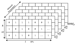
In this paper, we adapt the system model proposed in [9] for cellular MIMO networks to a CF system setting. Specifically, our system model consists of $L$ MIMO APs, each equipped with $M$ antennas, and $K$ single antenna UE. All units are placed randomly, in a uniform manner, on a limited Cartesian plane with a condition ensuring a minimum distance between any pair of units. We also assume that each UE can establish a time division duplex (TDD) link with each AP and that latency constraints allow deployment of a centralised RRM controller. We also introduce a concept of a tensor representation for the network. Shown in Fig. 1, the 3-dimensional array spans UE, APs and parameters of TDD links between aforementioned units. Most notably, the first parameter depicts connectivity, where $1$ and $0$ indicate whether $k$-th UE and $l$-th AP are connected or not. Consequentially it effects all parts of a system model containing sums over $k$ and $l$ indices.

Preserving the original definitions, in our system model $\tau_{c}$ denotes the length of coherence block, $\tau_{p}$ denotes the number of symbols for UL training, thus $\tau_{c}-\tau_{p}$ is available for transmitting data symbols. Fractions of the latter, $w_{l,k}^{\alpha}$, are used to tune the priorities of UL-DL transmissions between user $k$ and AP $l$. The wireless channels $\mathbf{h}_{l,k}\in\mathbb{C}^{M}$ are assumed to have Rayleigh fading with $\mathbf{h}_{k,l}\sim\mathcal{CN}\left(\mathbf{0},\mathbf{R}_{k,l}\right)$ distribution and correlation matrix $\mathbf{R}_{k,l}\in\mathbb{C}^{M\times M}$. The channel information is assumed to be known or easy to estimate. The TDD links consist of UL training and data transmission parts with definitions for closed-form UL-DL ergodic SE (1) and SINR (2) defined in accordance with [8, 9] and updated for CF setting as follows:

$$R_{l,k}^{\alpha}=w_{l,k}^{\alpha}\left(1-\frac{\tau_{p}}{\tau_{c}}\right)\log_{2}\left(1+\operatorname{SINR}_{l,k}^{\alpha}\right)$$ (1)

$$\operatorname{SINR}_{l,k}^{\alpha}=A\mathbin{/}(I_{C}^{\alpha}+I_{I}^{\alpha}+\sigma_{\alpha}^{2});$$ (2)

$$A=p_{l,k}^{\alpha}\left\|\boldsymbol{\psi}_{l,k}\right\|^{4}\operatorname{Tr}\left(\mathbf{R}_{l,k}\mathbf{F}_{l,k}^{-1}\mathbf{R}_{l,k}\right);$$

$$I_{C}^{\text{UL}}=\sum_{i,j\backslash l,k}p_{i,j}^{\text{UL}}\left|\boldsymbol{\psi}_{l,k}^{H}\boldsymbol{\psi}_{i,j}\right|^{2}\frac{\left|\operatorname{Tr}\left(\mathbf{R}_{i,j}\mathbf{F}_{l,k}^{-1}\mathbf{R}_{l,k}\right)\right|^{2}}{\operatorname{Tr}\left(\mathbf{R}_{l,k}\mathbf{F}_{l,k}^{-1}\mathbf{R}_{l,k}\right)};$$

$$I_{C}^{\text{DL}}=\sum_{i,j\backslash l,k}p_{i,j}^{\text{DL}}\left|\boldsymbol{\psi}_{l,k}^{H}\boldsymbol{\psi}_{i,j}\right|^{2}\frac{\left|\operatorname{Tr}\left(\mathbf{R}_{i,j}\mathbf{F}_{i,j}^{-1}\mathbf{R}_{l,k}\right)\right|^{2}}{\operatorname{Tr}\left(\mathbf{R}_{i,j}\mathbf{F}_{i,j}^{-1}\mathbf{R}_{i,j}\right)};$$

$$I_{I}^{\text{UL}}=\sum_{i,j\backslash l,k}p_{i,j}^{\text{UL}}\frac{\operatorname{Tr}\left(\mathbf{R}_{i,j}\mathbf{R}_{l,k}\mathbf{F}_{l,k}^{-1}\mathbf{R}_{l,k}\right)}{\operatorname{Tr}\left(\mathbf{R}_{l,k}\mathbf{F}_{l,k}^{-1}\mathbf{R}_{l,k}\right)};$$

$$I_{I}^{\text{DL}}=\sum_{i,j\backslash l,k}p_{i,j}^{\text{DL}}\frac{\operatorname{Tr}\left(\mathbf{R}_{i,j}\mathbf{F}_{i,j}^{-1}\mathbf{R}_{i,j}\mathbf{R}_{l,k}\right)}{\operatorname{Tr}\left(\mathbf{R}_{i,j}\mathbf{F}_{i,j}^{-1}\mathbf{R}_{i,j}\right)},$$

where $A$ denotes the array gain, $I_{C}^{\alpha}$ denotes the coherent interference (e.g. caused by pilot reuse), $I_{I}^{\alpha}$ is the incoherent interference and $\sigma_{\alpha}^{2}$ is the noise term.

Figure 1: Tensor representation of a CF network.

The rest of the model, which contributes to (1) follows the model proposed in [9], and is summarised as follows. During UL training, a number $K\leq\tau_{p}\leq KL$ of mutually orthogonal pilot signals $\boldsymbol{\psi}_{l,k}$ are reused among the UE and contribute to UL training pilot signal $\mathbf{Y}_{l,k}\in\mathbb{C}^{M\times\tau_{p}}$ at the AP as in (3).

$$\mathbf{Y}_{l,k}=\sum_{i,j}\mathbf{h}_{i,j}\boldsymbol{\psi}_{i,j}^{H}+\mathbf{N}_{l,k};$$ (3)

$$\hat{\mathbf{h}}_{l,k}=\left\|\boldsymbol{\psi}_{l,k}\right\|^{2}\mathbf{R}_{l,k}\left(\mathbf{F}_{l,k}\right)^{-1}\mathbf{Y}_{l,k}\boldsymbol{\psi}_{l,k};$$

$$\hat{\mathbf{h}}_{l,k}\sim\mathcal{CN}\left(\mathbf{0},\left\|\boldsymbol{\psi}_{l,k}\right\|^{4}\mathbf{R}_{l,k}\mathbf{F}_{l,k}^{-1}\mathbf{R}_{l,k}\right);$$

$$\mathbf{F}_{l,k}=\sum_{i,j}\mathbf{R}_{i,t}\left|\boldsymbol{\psi}_{i,j}^{H}\boldsymbol{\psi}_{l,k}\right|^{2}+\sigma_{\text{UL}}^{2}\left\|\boldsymbol{\psi}_{l,k}\right\|^{2}\mathbf{I}_{M},$$

where $\mathbf{N}_{l,k}\in\mathcal{CN}\left(\mathbf{0},\sigma_{\text{UL}}^{2}\mathbf{I}_{M\tau_{p}}\right)$ is the UL noise matrix with its elements sampled from $\mathcal{CN}\left({0},\sigma_{\text{UL}}^{2}\right)$ distribution and $\hat{\mathbf{h}}_{l,k}$ are channel estimates obtained by MMSE estimation [8, 9]. The resulting channel estimates shape linear processing vectors for data transmission. We make an assumption, that the timing difference between UE UL transmissions is insignificant, and they can be seen as practically simultaneous.

During data reception by the AP, the UL signal $\mathbf{v}_{l,k}^{H}\mathbf{y}_{l}$ is detected by applying maximum-ratio combining vector $\mathbf{v}_{l,k}$ (4)

$$\mathbf{v}_{l,k}^{H}\mathbf{y}_{l}=\sum_{i,t}\sqrt{p_{i,j}^{\text{UL}}}\hat{\mathbf{h}}_{l,k}^{H}\mathbf{h}_{i,j}s_{i,j}+\hat{\mathbf{h}}_{l,k}^{H}\mathbf{n}_{l},\ \mathbf{v}_{l,k}=\hat{\mathbf{h}}_{l,k};$$ (4)

$$\mathbf{y}_{l}=\sum_{i,j}\sqrt{p_{i,j}^{\text{UL}}}\mathbf{h}_{i,j}s_{i,j}+\mathbf{n}_{l},$$

where $\mathbf{y}_{l}$ is a received signal with $s_{l,k}$ complex data, $p_{l,k}^{\mathrm{UL}}$ – transmit data power and $\mathbf{n}_{l}\sim\mathcal{CN}\left(\mathbf{0},\sigma_{\text{UL}}^{2}\mathbf{I}_{M}\right)$ – noise term. In turn, UE receives a combined signal $r_{l,k}$ from all APs assigned to it, based on maximum ratio precoding vector $\mathbf{W}_{l,k}$.

$$r_{l,k}=\sum_{i,j}\sqrt{p_{i,j}^{\text{DL}}}\left(\mathbf{h}_{l,k}^{i}\right)^{H}\mathbf{w}_{i,j}q_{i,j}+n_{l,k};$$ (5)

$$\mathbf{w}_{l,k}=\hat{\mathbf{h}}_{l,k}\mathbin{/}{\sqrt{\left\|\boldsymbol{\psi}_{l,k}\right\|^{4}\operatorname{tr}\left(\mathbf{R}_{l,k}^{l}\mathbf{F}_{l,k}^{-1}\mathbf{R}_{l,k}^{l}\right)}};$$

$$\mathbf{x}_{l}=\sum_{j=1}^{K}\sqrt{p_{l,j}^{\text{DL}}}\mathbf{w}_{l,j}q_{l,j},$$

where $\mathbf{x}_{l}$ is a transmitted signal with $q_{l,k}$ complex data, $p_{l,k}^{\mathrm{UL}}$ – transmit data power and $n_{l,k}\sim\mathcal{CN}\left(0,\sigma_{\mathrm{dl}}^{2}\right)$ – noise term. Both (4) and (5) contribute directly to definition of SE in (1).

III Constrained Data Power Allocation

In this part we introduce a problem of data PC for the total max-min sum SE per user fairness under UL and DL transmit power constraints. The fractions $w_{l,k}^{\alpha}$, introduced earlier in Section II, from a system perspective serve not only as ratios between UL-DL symbol sequences, but also as prioritisations for each link established between $k$-th UE and $l$-th AP. We address the problem (6) in its original formulation [9]

$$\max_{w_{l,k}^{\alpha};\ p_{l,k}^{\alpha}\geq 0}\ \ \min_{(l,k)} R_{l,k}^{\text{UL}}+R_{l,k}^{\text{DL}}$$ (6)

s.t. $$p_{l,k}^{\text{UL}}\leq P_{\max,l,k}^{\text{UL}},\forall l,k$$

$$\sum_{k=1}^{K}p_{l,k}^{\text{DL}}\leq P_{\max,l}^{\text{DL}},\forall l\text{,}$$

where $P_{\max,l,k}^{\text{UL}},P_{\max,l}^{\text{DL}}$ are maximum powers that each UE and AP can allocate to in the UL and DL, respectively.

Because this task falls into the combinatorial domain over a large scalable parameter space, previous works applied various heuristics in combination with conventional optimisation methods. These methods treat the UL-DL terms of the objective function separately or use sequential iterations between pilot assignment and PC. In this work, we relax the constraint on $\boldsymbol{\psi}_{l,k}$ effectively leaving only PC for optimisation. In the context of CF MIMO networks, we must also ensure good scalability of the optimisation method as well as a good interpretability with uncertainty estimation for system simulations. BO allows to address all of the aforementioned points.

IV Multi-Objective Bayesian Optimisation

IV-A Preliminaries

BO is an efficient global black-box optimisation tool [13], that employs a probabilistic surrogate model in conjunction with an acquisition function to address the exploration-exploitation trade-off. This methodology has been successfully developed over the years to support multi-objective cases and to a lesser extent problems with noisy observations and parallelisation requirements.

Based on the formulation of constrained data PC (6), our objective, formally, is to find a set of optimal designs $\boldsymbol{x}$ over the bounded set $\mathcal{X}$ that maximise multiple objectives $\boldsymbol{f}(\boldsymbol{x})$. Here, multi-objective (MO) optimisation aims to identify a set of Pareto-optimal objective trade-offs. For example, a solution $\boldsymbol{f}(\boldsymbol{x})=\left[f^{(1)}(\boldsymbol{x}),\ldots,f^{(T)}(\boldsymbol{x})\right]$ dominates another solution $f(x)\succ f\left(x^{\prime}\right)$ if $f^{(t)}(\boldsymbol{x})\geq f^{(t)}\left(\boldsymbol{x}^{\prime}\right)$ for $t=1,\ldots,T$ and $\exists t\in\{1,\ldots,T\}$ s.t. $f^{(t)}(\boldsymbol{x})>f^{(t)}\left(\boldsymbol{x}^{\prime}\right)$. Then the Pareto frontier (PF) is defined as $\mathcal{P}^{*}=\left\{\boldsymbol{f}(\boldsymbol{x}):\boldsymbol{x}\in\mathcal{X},\nexists\ \boldsymbol{x}^{\prime}\in\mathcal{X}\right.$ s.t. $\left.\boldsymbol{f}\left(\boldsymbol{x}^{\prime}\right)\succ\boldsymbol{f}(\boldsymbol{x})\right\}$ with a set of optimal designs as $\mathcal{X}^{*}=\left\{\boldsymbol{x}:\boldsymbol{f}(\boldsymbol{x})\in\mathcal{P}^{*}\right\}$ . The PF often consists of an infinite set of points and MO optimisation algorithms aim to identify a finite approximate PF $\mathcal{P}$. The quality of PF is the hypervolume of the region of objective space that is dominated by the PF and bounded from below by a reference point [17].

Within the aforementioned framework each objective must be modelled as an independent surrogate function. GPs are typically used as such for BO due to their well-calibrated predictive uncertainty. Another part of BO is an acquisition function $\alpha(\cdot)$, that specifies value of evaluating a set of new points based on the surrogate’s predictive distribution. Surrogates substitute original objectives $\boldsymbol{f}$ with fast and computationally cheap evaluations. This allows to effectively run numerical optimisation methods to find $\boldsymbol{x}^{*}=\arg\max_{\boldsymbol{x}\in\mathcal{X}}\alpha(\boldsymbol{x})$ in the loop with a selection of new points for BO to update the model. Related research works contain many types of acquisition, which are chosen depending on the structure of the underlying problem [18, 19]. Some of acquisition functions are probability of improvement, entropy search, upper confidence bound, and expected hypervolume improvement (EHVI), where the latter is used in this work.

IV-B Expected Hypervolume Improvement

We first recall that the explanation of parallel MO BO solutions, devised by Daulton et al. [17], requires the definitions of the hypervolume indicator (HV) and hypervolume improvement (HVI).

The HV of a finite approximate PF $\mathcal{P}$ is the $T$-dimensional Lebesgue measure $\lambda_{T}$ of the space dominated by $\mathcal{P}$ and bounded from below by a reference point:

$$\boldsymbol{r}\in\mathbb{R}^{T}:\mathrm{HV}(\mathcal{P}\mid\boldsymbol{r})=\lambda_{T}\left(\bigcup_{\boldsymbol{v}\in\mathcal{P}}[\boldsymbol{r},\boldsymbol{v}]\right),$$ (7)

where $[\boldsymbol{r},\boldsymbol{v}]$ denotes the hyper-rectangle bounded by vertices $\boldsymbol{r}$ and $\boldsymbol{v}$. Then, the HVI of a set of points $\mathcal{P}^{\prime}$ with respect to an existing approximate PF $\mathcal{P}$ and reference point $\boldsymbol{r}$ are defined as $\mathrm{HVI}\left(\mathcal{P}^{\prime}\mid\mathcal{P},\boldsymbol{r}\right)=\mathrm{HV}\left(\mathcal{P}\cup\mathcal{P}^{\prime}\mid\boldsymbol{r}\right)-\mathrm{HV}(\mathcal{P}\mid\boldsymbol{r})$.

Since we approach our problem from black-box optimisation perspective, function values at unobserved points are unknown together with HVI of an out-of-sample point. BO remedies this issue by GP surrogates that provide a posterior distribution $p(\boldsymbol{f}(\boldsymbol{x})\mid\mathcal{D})$ over function values for each $\boldsymbol{x}$. This, in turn, allows to compute EHVI acquisition function analytically (8) or using Monte Carlo (MC) integration (9):

$$\alpha_{\mathrm{EHVI}}(\boldsymbol{x}\mid\mathcal{P})=\mathbb{E}[\mathrm{HVI}(\boldsymbol{f}(\boldsymbol{x})\mid\mathcal{P})]$$ (8)

$$\alpha_{q\mathrm{EHVI}}\left(\mathcal{X}_{\text{cand }}\mid\mathcal{P}\right)\approx\hat{\alpha}_{q\mathrm{EHVI}}\left(\mathcal{X}_{\text{cand }}\mid\mathcal{P}\right)=$$ (9)

$$\leavevmode\nobreak\ \leavevmode\nobreak\ =\frac{1}{N}\sum_{i=1}^{N}\operatorname{HVI}\left(\tilde{\boldsymbol{f}}_{i}\left(\mathcal{X}_{\text{cand }}\right)\mid\mathcal{P}\right),$$

where $\tilde{\boldsymbol{f}}_{i}\sim p(\boldsymbol{f}\mid\mathcal{D})$ and $\mathcal{X}_{\text{cand }}=\left\{x_{j}\right\}_{i=j}^{q}$.

IV-C Multi-Objective Noisy Expected Hypervolume Improvement

Because conventional BO does not scale well with number of objectives, and in such setting does not have converge guarantees, Daulton et al. [17] address that by deriving a Bayes-optimal EHVI criterion (10). This implies iterating the expectation over the posterior $p\left(\boldsymbol{f}\left(X_{n}\right)\mid\mathcal{D}_{n}\right)$ of the function values at previously evaluated data points $X_{n}$, given the noisy observations $\mathcal{D}_{n}=\left\{\boldsymbol{x}_{i},\boldsymbol{y}_{i},\left(\Sigma_{i}\right)\right\}_{i=1}^{n}$:

$$\alpha_{\mathrm{NEHVI}}(\boldsymbol{x})=\int\alpha_{\mathrm{EHVI}}\left(\boldsymbol{x}\mid\mathcal{P}_{n}\right)p\left(\boldsymbol{f}\mid\mathcal{D}_{n}\right)d\boldsymbol{f};$$ (10)

$$\hat{\alpha}_{\mathrm{NEHVI}}(\boldsymbol{x})=\frac{1}{N}\sum_{i=1}^{N}\operatorname{HVI}\left(\tilde{\boldsymbol{f}}_{i}(\boldsymbol{x})\mid\mathcal{P}_{i}\right),$$

where $P_{i}$ denotes the PF over $\boldsymbol{f}\left(X_{i}\right)$, $\tilde{\boldsymbol{f}}_{i}\left(X_{n},\boldsymbol{x}\right)\sim p\left(\boldsymbol{f}\left(X_{n},\boldsymbol{x}\right)\mid\mathcal{D}_{n}\right)$ is a joint posterior and $\hat{\alpha}_{\text{NEHVI}}(\boldsymbol{x})$ is an approximation of $\alpha_{\text{NEHVI}}(\boldsymbol{x})$ by MC integration. Note that in practice, the algorithm is computationally complex. Despite this, our interest lies primarily in the ability to support high-dimensional data PC, which naturally falls into the domain of BO with a noisy-EHVI acquisition function.

V Simulation Results

V-A Experimental Design

To demonstrate the performance of the proposed MO BO methodology, we consider three cases of CF networks, and one with a TDD link between a single UE and AP. In all settings, the APs are equipped with a 128 antenna MIMO system, while the UE s operate with single antennas. All units in the network are placed randomly with the following minimal distances between pairs: AP-UE– 40 m, UE-UE– 5 m, AP-AP– 100 m. Similarly to [9], there are $K$ orthogonal pilot signals and $P_{\max,l,k}^{\text{UL}}=200$ mW with $P_{\max,l,k}^{\text{DL}}=200K$ mW are set to ensure an equal total power budget for the UL and DL data transmissions. The covariance matrix of channel $\mathbf{R}_{l,k}$ (11) is defined according to the exponential correlation model for a uniform linear array:

$$\mathbf{R}_{l,k}=\beta_{l,k}\left[\begin{array}[]{ccc}1&\cdots&\left(r_{l,k}^{*}\right)^{M-1}\\ \vdots&\ddots&\vdots\\ \left(r_{l,k}\right)^{M-1}&\cdots&1\end{array}\right];$$ (11)

$$\beta_{l,k}[\mathrm{\leavevmode\nobreak\ dB}]=-148.1-37.6\log_{10}\left(d_{l,k}/1\mathrm{\leavevmode\nobreak\ km}\right)+z_{l,k},$$

where $\mu e^{j\theta_{l,k}}$ denotes the spatial correlation with $\mu$ in a closed unit interval, $\beta_{l,k}^{j}$ [dB] denotes the large-scale fading coefficients, $d_{l,k}$ denotes distance between respective UE and AP, and lastly $z_{l,k}$ is the log-normally distributed shadow fading term. Since we focus on the task of data PC, the pilot assignment is done according to the similarity between covariance matrices [20].

V-B Pareto Frontiers

To demonstrate the performance of a parallel MO BO scheme with EHVI [17] and gain insight into our multi-objective problem (6) at scale, we first consider three controllable experiments, which consist of finding PFs for a TDD link consisting of one UE and one AP.

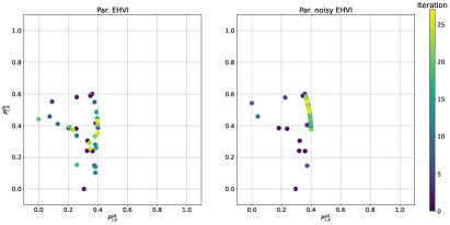
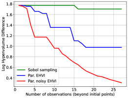
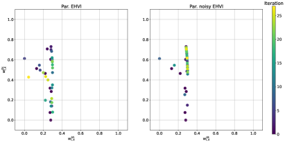
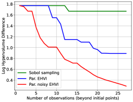
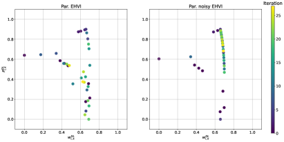
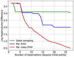
To this end, we first fix $w_{1,1}^{\mathrm{DL}}$ and $w_{1,1}^{\mathrm{UL}}$ by assigning random values to them, and optimise $P_{1,1}^{\mathrm{DL}}$ and $P_{1,1}^{\mathrm{UL}}$. Fig. (2) corresponds to this experiment, and contains the estimated PFs for EHVI and noisy-EHVI, as well as the convergence curves for the log-hypervolume difference, where they are compared with quasi-MC sampling, based on Sobol sequences. Next, in Fig. (3) and Fig. (4) we reverse the problem by optimising the pairs: $w_{1,k}^{\mathrm{DL}}$ with $w_{1,1}^{\mathrm{UL}}$ and $P_{1,k}^{\mathrm{DL}}$ with $w_{1,1}^{\mathrm{DL}}$, respectively.

The PFs contain the collected observations for both EHVI versions, where the colours correspond to the BO iteration, at which the point was collected. Across all Fig. 2-4, the central PFs for noisy-EHVI show that it is able to quickly identify the PF and most of its evaluations are very close to it. It is interesting to note that conventional EHVI also identifies multiple observations close to the PF, but due to relying on the technique of optimising random scalarisations, the shapes of PFs are less defined. Finally, notice that MC sampling is unable to converge to a PF, which is indicated by a stagnant log-hypervolume difference across all cases. It is worth mentioning that the noisy-EHVI continues to converge, and has a potential to approximate more complex PF, which aligns with its convergence properties, as established in [17].

Further controllable experiments (not reported here) provide additional intuition into performance of the chosen MO optimisation methods, but our main goal is to maximise total SE by solving data PC.

Figure 2: PFs for $P_{l,k}^{\text{DL}}$ and $P_{l,k}^{\text{UL}}$ using EHVI with log-hypervolume difference convergence plot, 1 UE– 1 AP.

å

Figure 3: PFs for $w_{l,k}^{\text{DL}}$ and $w_{l,k}^{\text{UL}}$ using EHVI with log-hypervolume difference convergence plot, 1 UE– 1 AP.

Figure 4: PFs for $w_{l,k}^{\text{DL}}$ and $P_{l,k}^{\text{DL}}$ using EHVI with log-hypervolume difference convergence plot, 1 UE– 1 AP.

V-C Spectral Efficiencies

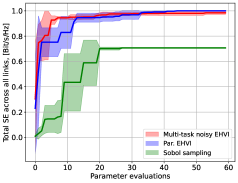
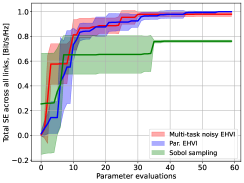
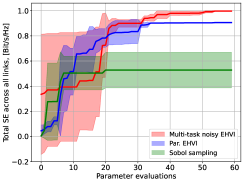
In the key set of results reported below, we provide convergence plots with uncertainty estimates for SE maximisation via data PC in three scenarios with increasing CF network dimensionality. Similarly to sub-section (V-A), we also compare quasi-MC sampling and two EHVI variants [17].

Fig. 5(a), 5(b) and 5(c) show the total or summed SE for all established UE-AP links in the network for problem (6). The normalisation is done in order to compare the convergence processes in relation with the number of parameter evaluations across all three network cases.

The first case only contains 5 UE s and 5 AP s, which is comparable to the number of units in previous works [8, 9]. Here, both versions of EHVI show similar performance by reaching a PF solution after 20 parameter evaluations. The real benefit of noisy-EHVI becomes apparent in large scenarios containing in total 50 and 100 units in the network. There, conventional methods do not scale well and random sampling struggles to continue convergence. Fig. 5(c) confirms this notion, as quasi-MC maintains high uncertainty through all evaluations, while the noisy-EHVI continuously reduces.

Because studied problem is multi-objective and combinatorial in its nature, it is difficult to know the exact optimum. In context of future ressearch, it would be crucial to utilise high interpretability of BO in combination with PFs in order to assess properties of solution on per UE basis.

(a) 5 UE, 5 AP

(b) 30 UE, 20 AP

(c) 60 UE, 40 AP

Figure 5: Convergence rates for total spectral efficiency as a function of $w_{l,k}^{\alpha}$ and $p_{l,k}^{\alpha}$ for 3 network cases.

VI Concluding Remarks and Future Research

In this paper, we have described and shown a solution to the data PC problem in a CF setting, using an advanced BO engine of the multi-objective noisy-EHVI.

Despite the fact that nature of the problem does not allow to explicitly analyse the convergence towards the global optimum or a unique PF, MO BO provides various benefits, which make its application advantageous in the domain of RRM. For example, BO can be used to emulate the behaviour of large scale dynamical networks, effectively replacing existing link-level simulators. Another advantage of the Bayesian approach is its modularity, which allows to combine GP nonparametric and parametric models and build statistical emulators.

A statistical emulator is an effective data-driven model that learns about a given simulation. Most notably, it learns with uncertainty. In practice, the emulators may replace simulators, and they can invoke the simulator to make updates. A statistical emulator is also a system that reconstructs the simulation with a statistical model. Together with reconstruction, a statistical emulator can be used to correlate with the real environment as well as calibrate the simulation to the environment. This allows the emulator to characterise where the simulation can be relied on and consequentially to adjudicate between simulations. This is known as multi-fidelity emulation.

Based on the aforementioned properties and results, we envision a future work in the context of MIMO CF network emulators, which will not be hindered by scalability or restrictions in terms of the tunable parameters.

References

- [1] V. Ranjbar, A. Girycki, M. A. Rahman, S. Pollin, M. Moonen, and E. Vinogradov, “Cell-Free mMIMO Support in the O-RAN Architecture: A PHY Layer Perspective for 5G and Beyond Networks,” IEEE Communications Standards Magazine, vol. 6, no. 1, pp. 28–34, Mar. 2022.
- [2] S. Chen, J. Zhang, J. Zhang, E. Björnson, and B. Ai, “A survey on user-centric cell-free massive MIMO systems,” Digital Communications and Networks, Dec. 2021.
- [3] I. M. Braga, R. P. Antonioli, G. Fodor, Y. C. B. Silva, and W. C. Freitas, “Joint Pilot and Data Power Control Optimization in the Uplink of User-Centric Cell-Free Systems,” IEEE Communications Letters, vol. 26, no. 2, pp. 399–403, Feb. 2022.
- [4] S. Wu, Y. Wei, S. Zhang, and W. Meng, “Proportional-Fair Resource Allocation for User-Centric Networks,” IEEE Transactions on Vehicular Technology, vol. 71, no. 2, pp. 1549–1561, Feb. 2022.
- [5] Y. S. Nasir and D. Guo, “Deep Reinforcement Learning for Joint Spectrum and Power Allocation in Cellular Networks,” in 2021 IEEE Globecom Workshops (GC Wkshps), Dec. 2021, pp. 1–6.
- [6] V. Saxena, H. Tullberg, and J. Jaldén, “Reinforcement Learning for Efficient and Tuning-Free Link Adaptation,” IEEE Transactions on Wireless Communications, vol. 21, no. 2, pp. 768–780, Feb. 2022.
- [7] A. M. Girgis, J. Park, M. Bennis, and M. Debbah, “Predictive Control and Communication Co-Design via Two-Way Gaussian Process Regression and AoI-Aware Scheduling,” IEEE Transactions on Communications, vol. 69, no. 10, pp. 7077–7093, Oct. 2021.
- [8] T. Van Chien, E. Björnson, and E. G. Larsson, “Joint Pilot Design and Uplink Power Allocation in Multi-Cell Massive MIMO Systems,” IEEE Transactions on Wireless Communications, vol. 17, no. 3, pp. 2000–2015, Mar. 2018.
- [9] T. H. Nguyen, T. V. Chien, H. Q. Ngo, X. N. Tran, and E. Björnson, “Pilot Assignment for Joint Uplink-Downlink Spectral Efficiency Enhancement in Massive MIMO Systems With Spatial Correlation,” IEEE Transactions on Vehicular Technology, vol. 70, no. 8, pp. 8292–8297, Aug. 2021.
- [10] T. Wang and S. Wang, “Inter-Slice Radio Resource Allocation: An Online Convex Optimization Approach,” IEEE Wireless Communications, vol. 28, no. 5, pp. 171–177, Oct. 2021.
- [11] Y. Li, J. Jiang, C. Jia, Y. Yuan, Z. Zhao, Y. Du, and Z. Wang, “Deep Reinforcement Learning-Based Multi-Panel Beam Management in Massive MIMO Systems: Algorithm Design and System-Level Simulation,” in 2021 IEEE 32nd Annual International Symposium on Personal, Indoor and Mobile Radio Communications (PIMRC), Sep. 2021, pp. 1–6.
- [12] R. M. Dreifuerst, S. Daulton, Y. Qian, P. Varkey, M. Balandat, S. Kasturia, A. Tomar, A. Yazdan, V. Ponnampalam, and R. W. Heath, “Optimizing Coverage and Capacity in Cellular Networks using Machine Learning,” in ICASSP 2021 - 2021 IEEE International Conference on Acoustics, Speech and Signal Processing (ICASSP), Jun. 2021, pp. 8138–8142.
- [13] L. Maggi, A. Valcarce, and J. Hoydis, “Bayesian Optimization for Radio Resource Management: Open Loop Power Control,” IEEE Journal on Selected Areas in Communications, vol. 39, no. 7, pp. 1858–1871, Jul. 2021.
- [14] L. Eller, V. Raida, P. Svoboda, and M. Rupp, “Localizing Basestations From End-User Timing Advance Measurements,” IEEE Access, vol. 10, pp. 5533–5544, 2022.
- [15] E. Tekgul, T. Novlan, S. Akoum, and J. G. Andrews, “Sample-Efficient Learning of Cellular Antenna Parameter Settings,” in 2021 IEEE Information Theory Workshop (ITW), Oct. 2021, pp. 1–6.
- [16] W. Maddox, Q. Feng, and M. Balandat, “Optimizing High-Dimensional Physics Simulations via Composite Bayesian Optimization,” arXiv:2111.14911 [cs], Nov. 2021.
- [17] S. Daulton, M. Balandat, and E. Bakshy, “Parallel Bayesian Optimization of Multiple Noisy Objectives with Expected Hypervolume Improvement,” in Advances in Neural Information Processing Systems, vol. 34. Curran Associates, Inc., 2021, pp. 2187–2200.
- [18] J. Wilson, F. Hutter, and M. Deisenroth, “Maximizing acquisition functions for Bayesian optimization,” in Advances in Neural Information Processing Systems, vol. 31. Curran Associates, Inc., 2018.
- [19] R. B. Gramacy, Surrogates: Gaussian Process Modeling, Design, and Optimization for the Applied Sciences, 1st ed. Boca Raton: Chapman and Hall/CRC, Jan. 2020.
- [20] L. You and X. Gao, “Pilot Reuse for Massive MIMO,” in Encyclopedia of Wireless Networks, X. S. Shen, X. Lin, and K. Zhang, Eds. Cham: Springer International Publishing, 2020, pp. 1071–1073.