An example of higher-dimensional Heegaard Floer homology

Abstract.

We count pseudoholomorphic curves in the higher-dimensional Heegaard Floer homology of disjoint cotangent fibers of a two dimensional disk. We show that the resulting algebra is isomorphic to the Hecke algebra associated to the symmetric group.

1. Introduction

Many topological properties of a manifold $M$ can be recovered from the symplectic geometry of its cotangent bundle $T^{*}M$. An example is the $A_{\infty}$-equivalence between the wrapped Floer homology $CW^{*}(T^{*}_{q}M)$ of a cotangent fiber and the space $C_{-*}(\Omega_{q}M)$ of chains on the based loop space of $M$, proved by Abbondandolo, Schwarz [AS10] and Abouzaid [Abo12].

On the symplectic side, there is a generalization, the wrapped Floer homology $CW^{*}(\sqcup_{i=1}^{\kappa}T^{*}_{q_{i}}M)$ of $\kappa$ disjoint cotangent fibers in the framework of higher-dimensional Heegaard Floer homology (abbreviated HDHF) established by Colin, Honda and Tian [CHT20]. It is related to the braid group of $M$ on the topological side.

When $M=\Sigma$ is a real oriented surface, the HDHF was recently studied by Honda, Tian and Yuan [HTY22]. Pick $\kappa$ basepoints $\mathbf{q}=\{q_{1},\dots,q_{\kappa}\}\subset\Sigma$. By definition, $CW^{*}(\sqcup_{i}T^{*}_{q_{i}}\Sigma)$ is an $A_{\infty}$ algebra over $\mathbb{Z}[[\hbar]]$, where $\hbar$ keeps track of the Euler characteristic of the holomorphic curves that are counted in the definition of the $A_{\infty}$-operations. If $\Sigma$ is not a two sphere, then $CW^{*}(\sqcup_{i}T^{*}_{q_{i}}\Sigma)$ is supported in degree zero and hence is an ordinary algebra. The main result of [HTY22] is that the algebra $CW^{*}(\sqcup_{i}T^{*}_{q_{i}}\Sigma)$ is isomorphic to the braid skein algebra $\operatorname{BSk}_{\kappa}(\Sigma)$ of $\Sigma$, which was defined by Morton and Samuelson [MS21]. Roughly speaking, $\operatorname{BSk}_{\kappa}(\Sigma)$ is a quotient of the group algebra of the braid group of $\Sigma$ by the HOMFLY skein relation which is expressed in terms of $\hbar$. The skein relation has an explanation as holomorphic curve counting due to Ekholm and Shende [ES19]. This is one of the keys to build the bridge between $CW^{*}(\sqcup_{i}T^{*}_{q_{i}}\Sigma)$ and $\operatorname{BSk}_{\kappa}(\Sigma)$.

Morton and Samuelson showed that $\operatorname{BSk}_{\kappa}(\Sigma)$ is isomorphic to the double affine Hecke algebra associated to $\mathfrak{gl}_{\kappa}$ when $\Sigma$ is a torus. Based on this result, Honda, Tian and Yuan proved the isomorphisms between $CW^{*}(\sqcup_{i}T^{*}_{q_{i}}\Sigma)$ and various Hecke algebras of type A for $\Sigma$ being a disk, a cylinder or a torus.

In this paper, we focus on the local case: $\Sigma=D^{2}$ is a disk. Let $\operatorname{End}(L^{\otimes\kappa})$ denote the algebra $CW^{*}(\sqcup_{i}T^{*}_{q_{i}}D^{2})$ throughout the paper. It is isomorphic to the finite Hecke algebra associated to the symmetric group $S_{\kappa}$ over $\mathbb{Z}[[\hbar]]$ [HTY22]. The main result of this paper is to show that $\operatorname{End}(L^{\otimes\kappa})$ can be defined over $\mathbb{Z}[\hbar]$, and the isomorphism to the finite Hecke algebra still holds.

By definition, the Floer generators of $\operatorname{End}(L^{\otimes\kappa})$ are tuples of intersection points between the cotangent fibers $T^{*}_{q_{i}}D^{2}$. They are in one-to-one correspondence to elements of the symmetric group $S_{\kappa}$. Let $T_{w}\in\operatorname{End}(L^{\otimes\kappa})$ denote the corresponding Floer generator for $w\in S_{\kappa}$.

We now recall some basic facts about the Hecke algebra associated to $S_{\kappa}$. For our purpose, we change the variable from $q$ to $\hbar$ via $\hbar=q-q^{-1}$.

Definition 1.1.

The Hecke algebra $H_{\kappa}$ is a unital $\mathbb{Z}[\hbar]$-algebra generated by $\tilde{T}_{1},\dots,\tilde{T}_{\kappa-1}$, with relations

$$\tilde{T}_{i}^{2} =1+\hbar\tilde{T}_{i},$$

$$\tilde{T}_{i}\tilde{T}_{j} =\tilde{T}_{j}\tilde{T}_{i}\,\,\,\mathrm{for}\,\,\,|i-j|>1,$$

$$\tilde{T}_{i}\tilde{T}_{i+1}\tilde{T}_{i} =\tilde{T}_{i+1}\tilde{T}_{i}\tilde{T}_{i+1}.$$

It is known that the Hecke algebra $H_{\kappa}$ is a free $\mathbb{Z}[\hbar]$-module with a basis $\tilde{T}_{w},w\in S_{\kappa}$, called the standard basis. Here, $\tilde{T}_{i}=\tilde{T}_{s_{i}}$ for the transposition $s_{i}=(i,i+1)$. There is a length function on $S_{\kappa}$ defined by $l(w)=\min\{l\leavevmode\nobreak\ |\leavevmode\nobreak\ w=s_{i_{1}}\cdots s_{i_{l}}\}$. The basis $\tilde{T}_{w}=\tilde{T}_{i_{1}}\cdots\tilde{T}_{i_{l}}$ if $w=s_{i_{1}}\cdots s_{i_{l}}$ is an expression of minimal length. Moreover, the algebra structure on $H_{\kappa}$ is uniquely determined by

(1.3) $$\tilde{T}_{i}\tilde{T}_{w}=\left\{\begin{array}[]{ll}\tilde{T}_{s_{i}w}&\mathrm{if}\,\,\,l(s_{i}w)>l(w)+1\\ \tilde{T}_{s_{i}w}+\hbar\tilde{T}_{w}&\mathrm{if}\,\,\,l(s_{i}w)<l(w)-1\end{array}\right.$$

Our main result is the following.

Theorem 1.2.

The HDHF homology $\operatorname{End}(L^{\otimes\kappa})$ is defined over $\mathbb{Z}[\hbar]$. Moreover, there is an isomorphism of unital algberas $\phi:H_{\kappa}\to\operatorname{End}(L^{\otimes\kappa})$ such that $\phi(\tilde{T}_{w})=T_{w}$ for $w\in S_{\kappa}$.

Our strategy of the proof is a direct computation of HDHF. It is different from the method in [HTY22]. For the convenience of curve counting, we view the disk $D^{2}$ as a product of two intervals $I_{1}\times I_{2}$ so that $T^{*}D^{2}=T^{*}I_{1}\times T^{*}I_{2}\subset\mathbb{C}\times\mathbb{C}$. Lagrangians (wrapped cotangent fibers) are products of 1-dimensional Lagrangians in $T^{*}I_{1}$ and $T^{*}I_{2}$. Counting curves in $T^{*}D^{2}$ is then reduced to counting curves in $\mathbb{C}$, which is easier to work with.

Further directions:

It is natural to ask whether the HDHF homology $\operatorname{End}(\sqcup_{i}T^{*}_{q_{i}}\Sigma)$ of disjoint fibers of $T^{*}\Sigma$ can be defined over $\mathbb{Z}[\hbar]$ for a general surface $\Sigma$. It is possible to generalize our local result to the global case by using some sheaf theoretic technique, for instance in [GPS18].

It is also interesting to explain the geometric meaning of the change of variables $\hbar=q-q^{-1}$. Note that the canonical basis of the Hecke algebra is defined over $\mathbb{Z}[q,q^{-1}]$. We will express the canonical basis via HDHF in an upcoming paper.

Acknowledgements. The authors thank Ko Honda for numerous ideas and suggestions. YT is supported by NSFC 11971256.

2. Preliminaries

We first specify the ambient manifold and Lagrangian submanifolds of interest. For convenience of curve counting, we set $D^{2}=I_{1}\times I_{2}$ with $I_{1}=I_{2}=[0,1]$, which is topologically the same as the unit disk. Let $X=T^{*}D^{2}=T^{*}I_{1}\times T^{*}I_{2}$ be the total space of the cotangent bundle of $D^{2}$.

Consider the canonical Liouville form $\theta$ on $T^{*}D^{2}$, which induces a contact manifold structure at the infinity of $(T^{*}D^{2},\theta)$. For a Lagrangian $L\subset{T^{*}D^{2}}$, denote its boundary at infinity by $\partial_{\infty}L$. An isotopy of Lagrangians $L_{t}$ in $T^{*}D^{2}$ is called positive if $\alpha(\partial_{t}\partial_{\infty}L_{t})>0$ for all $t$. Let $T^{*}_{v}D^{2}=T^{*}D^{2}|_{\partial D^{2}}$ be the vertical boundary of $T^{*}D^{2}$ over $\partial D^{2}$. We require that any isotopy $L_{t}$ cannot cross $T_{v}^{*}D^{2}$. A positive isotopy is also called a “partially wrapping”. For the details of partially wrapped Fukaya categories, we refer to [Syl19] by Sylvan and [GPS20] by Ganatra, Shende, and Pardon.

We next consider the generalization to wrapped HDHF. Pick $\kappa$ disjoint basepoints $\mathbf{q}=\{q_{1},\dots,q_{\kappa}\}\subset D^{2}\backslash\partial D^{2}$ and consider the $\kappa$ cotangent fibers $L_{0i}=T^{*}_{q_{i}}D$ for $i=1,\dots,\kappa$. We denote $\mathcal{L}_{0}=\{L_{01},\dots,L_{0\kappa}\}$. An isotopy of $\kappa$-tuple of Lagrangians $\mathcal{L}_{t}=\{L_{t1},\dots,L_{t\kappa}\}$ is called positive if $\alpha(\partial_{t}\partial_{\infty}L_{ti})>0$ for all $i=1,\dots,\kappa$ and all $t$. For a pair of $\kappa$-tuples of Lagrangians $\mathcal{A}$ and $\mathcal{B}$, we denote $\mathcal{A}\rightsquigarrow\mathcal{B}$ if there is an positive isotopy from $\mathcal{A}$ to $\mathcal{B}$.

We then perform positive wrapping on $\mathcal{L}_{0}$ to get $\mathcal{L}_{j}=\{L_{j1},\dots,L_{j\kappa}\}$ for $j=1,2$. Specifically, we put $\mathcal{L}_{0},\mathcal{L}_{1},\mathcal{L}_{2}$ in the position as in Figure 1 (b,c), which represent the $T^{*}I_{1}$-direction and $T^{*}I_{2}$-direction, respectively. It is easy to check that

$$\mathcal{L}_{0}\rightsquigarrow\mathcal{L}_{1}\rightsquigarrow\mathcal{L}_{2}.$$

Remark 2.1.

We fix this special wrapping of $\mathcal{L}_{0},\mathcal{L}_{1},\mathcal{L}_{2}$. It is crucial for our counting of curves. We do not know whether the finite generation over $\hbar$ still holds for a general wrapping.

The HDHF cochain complex $CW^{*}(\mathcal{L}_{i},\mathcal{L}_{j})$, $i<j$ is defined as the free abelian group generated by $\kappa$-tuples of intersection points between $\mathcal{L}_{i}$ and $\mathcal{L}_{j}$ over $\mathbb{Z}[[\hbar]]$. By definition, $CW^{*}(\mathcal{L}_{i},\mathcal{L}_{j})$ is an $A_{\infty}$-algebra. We refer the reader to [HTY22] for details of the definition of HDHF in this case.

There is an absolute grading on $CW^{*}(\mathcal{L}_{i},\mathcal{L}_{j})$ and the degree is supported at $0$ by [HTY22, Proposition 2.9]. Hence, $CW^{*}(\mathcal{L}_{i},\mathcal{L}_{j})$ is an ordinary algebra over $\mathbb{Z}[[\hbar]]$. We denote it by $\operatorname{End}(L^{\otimes\kappa})$.

We describe the $m_{2}$-composition map of $\operatorname{End}(L^{\otimes\kappa})$ in the following. We set $\widehat{X}=D_{3}\times X$ as the target manifold, where $D_{3}$ is the unit disk with 3 boundary punctures and referred as the “$A_{\infty}$ base direction”. Let $z_{0},z_{1},z_{2}$ be the boundary punctures of $D_{3}$ and let $\alpha_{0},\alpha_{1},\alpha_{2}$ be the boundary arcs. We extend $\mathcal{L}_{i}$ to the $D_{3}$ direction by setting $\widehat{\mathcal{L}}_{i}=\alpha_{i}\times\mathcal{L}_{i}$, $\widehat{L}_{ij}=\alpha_{i}\times L_{ij}$, $i=0,1,2$, $j=1,\dots,\kappa$, which are Lagrangian submanifolds of $\widehat{X}$.

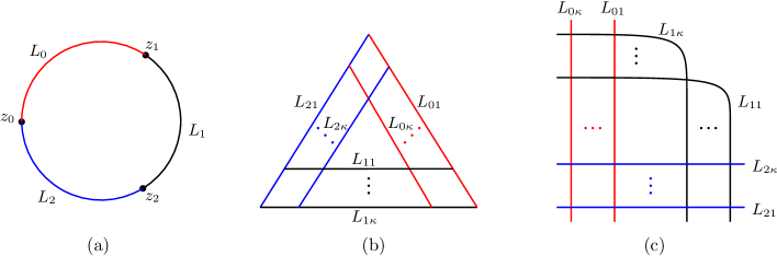
Figure 1. (a) $D_{3}$, the $A_{\infty}$ base direction; (b) The Lagrangians in the $T^{*}I_{1}$ direction; (c) The Lagrangians in the $T^{*}I_{2}$ direction.

For $i=0,1,2$, let $\boldsymbol{y}_{i}=\{y_{i1},\dots,y_{i\kappa}\}$ be a tuple of intersection points $y_{ij}\in\widehat{L}_{(i-1)j}\cap\widehat{L}_{ij^{\prime}}$, where $\{1^{\prime},\dots,\kappa^{\prime}\}$ is some permutation of $\{1,\dots,\kappa\}$. Let $J$ be a small generic perturbation of $J_{D_{3}}\times J_{1}\times J_{2}$, where $J_{D_{3}},J_{1},J_{2}$ are the standard complex structures on $D_{3},T^{*}I_{1},T^{*}I_{2}$, viewed as subsets of $\mathbb{C}$. Let $\mathcal{M}_{J}(\boldsymbol{y}_{1},\boldsymbol{y}_{2},\boldsymbol{y}_{0})$ be the moduli space of maps

(2.1) $$u:(\dot{F},j)\to(\widehat{X},J),$$

where $(F,j)$ is a compact Riemann surface with boundary, $\boldsymbol{p}_{i}$ are disjoint tuples of boundary punctures of $F$ for $i=0,1,2$, and $\dot{F}=F\backslash\cup_{i}\boldsymbol{p}_{i}$. The map $u$ satisfies

(2.7) $$\left\{\begin{array}[]{ll}\text{$du\circ j=J\circ du$;}\\ \text{each component of $\partial\dot{F}$ is mapped to a unique $\widehat{L}_{ij}$;}\\ \text{$\pi_{X}\circ u$ tends to $\boldsymbol{y}_{i}$ as $s_{i}\to+\infty$ for $i=1,\dots,m$;}\\ \text{$\pi_{X}\circ u$ tends to $\boldsymbol{y}_{0}$ as $s_{0}\to-\infty$;}\\ \text{$\pi_{D_{3}}\circ u$ is a $\kappa$-fold branched cover of $D_{3}$,}\end{array}\right.$$

where the 3rd condition means that $\pi_{X}\circ u$ maps the neighborhoods of the punctures of $\boldsymbol{p}_{i}$ asymptotically to the Reeb chords of $\boldsymbol{y}_{i}$ for $i=1,\dots,m$ at the positive ends. The 4th condition is similar.

The $m_{2}$-composition map of $\operatorname{End}(L^{\otimes\kappa})$ is then defined as

(2.8) $$m_{2}(\boldsymbol{y_{1}},\boldsymbol{y_{2}})=\sum_{\boldsymbol{y_{0}},\chi\leq\kappa}\#\mathcal{M}^{\mathrm{ind}=0,\chi}_{J}(\boldsymbol{y_{1}},\boldsymbol{y_{2}},\boldsymbol{y_{0}})\cdot\hbar^{\kappa-\chi}\cdot\boldsymbol{y_{0}}.$$

where the superscript “$\mathrm{ind}$” denotes the Fredholm index and “$\chi$” denotes the Euler characteristic of $F$; the symbol $\#$ denotes the signed count of the corresponding moduli space.

It is known that a choice of spin structures on the Lagrangians determines a canonical orientation of the moduli space. The Lagrangian in our case is the cotangent fiber which is topologically $\mathbb{R}^{2}$. So there is a unique spin structure. We omit the details about the orientation, and refer the reader to [CHT20, Section 3].

3. The case of $\kappa=2$

In this section we compute $\operatorname{End}(L^{\otimes 2})$ as a model case. The general case will be discussed in Section 4.

For $0\leq i<j\leq 2$, there are two Floer generators of $CF^{*}(\mathcal{L}_{i},\mathcal{L}_{j})$: $T_{{\operatorname{id}}}$ and $T_{1}$, where $T_{{\operatorname{id}}}=(q_{1},q_{2})$ with $q_{1}\in L_{i1}\cap L_{j1}$ and $q_{2}\in L_{i2}\cap L_{j2}$, and $T_{1}=(q_{1},q_{2})$ with $q_{1}\in L_{i1}\cap L_{j2}$ and $q_{2}\in L_{i2}\cap L_{j1}$. The main result of this section is the following.

Proposition 3.1.

The multiplication on $\operatorname{End}(L^{\otimes 2})$ is given by

$$T_{\operatorname{id}}\cdot T_{\operatorname{id}} =T_{\operatorname{id}};$$

$$T_{\operatorname{id}}\cdot T_{1} =T_{1};$$

$$T_{1}\cdot T_{\operatorname{id}} =T_{1};$$

$$T_{1}\cdot T_{1} =1+\hbar T_{1}.$$

Hence, Theorem 1.2 holds for $\kappa=2$.

The proof of this proposition occupies the rest of the section. We directly compute the moduli spaces. There are trivial curves with $\chi=2$ accounting for the $\hbar^{0}$ terms in the multiplication. We show that $\mathcal{M}^{\chi<2}_{J}(\boldsymbol{y}_{1},\boldsymbol{y}_{2},\boldsymbol{y}_{0})=\emptyset$ for almost all cases except that $\mathcal{M}^{\chi=1}_{J}(T_{1},T_{1},T_{1})\neq\emptyset$ accounting for the $\hbar^{1}$ term in $T_{1}\cdot T_{1}$. The main strategy to prove the nonexistence of curves is to stretch the Lagrangians in the $T^{*}I_{1}$-direction and apply the Gromov compactness.

For later use, we make the following conventions:

• We denote the length of the line segment of $L_{1\kappa}$ in the $I_{1}$-direction by $d$, see Figure 1(b);

• For $q\in X$, we denote its projection in the $T^{*}I_{1}$ (resp. $T^{*}I_{2}$)-direction by $q^{\prime}$ (resp. $q^{\prime\prime}$).

• We denote the line segment between $q_{1}$ and $q_{2}$ by $(q_{1}q_{2})$.

• When plotting figures, we denote the intersections $q_{i}$ by $i$.

• When taking the limit, we denote the degenerated domain by $\dot{F}^{\prime}$ and its irreducible component containing $\{p_{1},p_{2},\dots\}$ by $\dot{F}^{\prime}_{(12\dots)}$.

Lemma 3.2.

$T_{\operatorname{id}}\cdot T_{\operatorname{id}}=T_{\operatorname{id}}$.

Proof.

We first show that

(3.1) $$\#\mathcal{M}^{\chi}_{J}(T_{\operatorname{id}},T_{\operatorname{id}},T_{\operatorname{id}})=\left\{\begin{array}[]{lr}1,\,\,\chi=2&\\ 0,\,\,\chi<2&\end{array}.\right.$$

The Floer generators are shown in Figure 2.

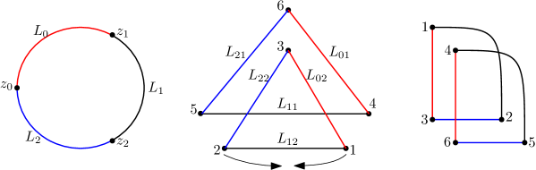
Figure 2. Generators for $\mathcal{M}_{J}(T_{\operatorname{id}},T_{\operatorname{id}},T_{\operatorname{id}})$.

If $\chi=2$, there is a unique trivial holomorphic curve consisting of two disks. So $\#\mathcal{M}^{\chi=2}_{J}(T_{\operatorname{id}},T_{\operatorname{id}},T_{\operatorname{id}})=1$.

If $\chi<2$, let $d\to 0$, i.e., let $q^{\prime}_{1}$ and $q^{\prime}_{2}$ get closer. In the limit, since there is no slit or branch points separating $q^{\prime}_{1}$ and $q^{\prime}_{2}$, $\dot{F}^{\prime}_{(12)}$ bubbles off as a triangle with vertices $\{p_{1},p_{2},p_{a}\}$, where $\{p_{a}\}$ is a boundary nodal point. The projection of $\dot{F}^{\prime}_{(12)}$ under $\pi_{T^{*}I_{2}}\circ u$ is a homeomorphism to the triangle with vertices $\{q^{\prime\prime}_{1},q^{\prime\prime}_{2},q^{\prime\prime}_{3}\}$. Hence the projection of $\dot{F}^{\prime}_{(3)}$ under $\pi_{T^{*}I_{2}}\circ u$ is a constant map to $q^{\prime\prime}_{3}$. Since $\pi_{T^{*}I_{2}}\circ u$ is of degree 0 or 1 near $q^{\prime\prime}_{3}$, the image $\pi_{T^{*}I_{2}}\circ u(\dot{F}\backslash(\dot{F}^{\prime}_{(12)}\cup\dot{F}^{\prime}_{(3)}))$ is disjoint from $q^{\prime\prime}_{3}$. It follows that $\dot{F}^{\prime}_{(12)}\cup\dot{F}^{\prime}_{(3)}$ is a connected component of $\dot{F}^{\prime}$. Therefore, $\dot{F}$ consists of two components before the degeneration, which are homeomorphically mapped to the triangles $\{q^{\prime\prime}_{1},q^{\prime\prime}_{2},q^{\prime\prime}_{3}\}$ and $\{q^{\prime\prime}_{4},q^{\prime\prime}_{5},q^{\prime\prime}_{6}\}$ under $\pi_{T^{*}I_{2}}\circ u$, respectively. So $\chi=2$, which is a contradiction. We conclude that $\#\mathcal{M}^{\chi}_{J}(T_{\operatorname{id}},T_{\operatorname{id}},T_{\operatorname{id}})=0$ if $\chi<2$.

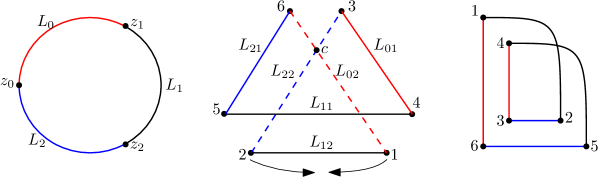
Figure 3. Generators for $\mathcal{M}_{J}(T_{\operatorname{id}},T_{\operatorname{id}},T_{1})$.

We next show that $\#\mathcal{M}_{J}(T_{\operatorname{id}},T_{\operatorname{id}},T_{1})=0$. The generators are shown in Figure 3. As $d\to 0$, $\dot{F}^{\prime}_{(12)}$ bubbles off as a triangle with vertices $\{p_{1},p_{2},p_{a}\}$, where $p_{a}\in\dot{F}^{\prime}$ is a nodal point. Denote the union of irreducible components of $\dot{F}^{\prime}$ containing the preimage of the dashed lines in the $T^{*}I_{1}$-direction by $\dot{F}^{\prime}_{\text{dash}}$. Since $p_{3}$, $p_{6}$, and $p_{a}$ are mapped to $z_{0}$ under $\pi_{D_{3}}\circ u$ in the limit, the preimages of the dashed lines are also mapped to $z_{0}$. Hence, $\dot{F}^{\prime}_{\text{dash}}$ is mapped to the constant point $z_{0}$ under $\pi_{D_{3}}\circ u$. Since $(q^{\prime}_{5}q^{\prime}_{6})$ cannot be separated by slits, we have $q^{\prime}_{5}\in\dot{F}^{\prime}_{\text{dash}}$ and $\pi_{D_{3}}\circ u(q^{\prime}_{5})=z_{0}$. This contradicts with the fact that $\pi_{D_{3}}\circ u(q^{\prime}_{5})=z_{2}$. Therefore, $\mathcal{M}_{J}(T_{\operatorname{id}},T_{\operatorname{id}},T_{1})=\emptyset$. ∎

Lemma 3.3.

$T_{\operatorname{id}}\cdot T_{1}=T_{1}$.

Proof.

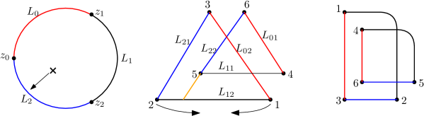
Figure 4. Generators for $\mathcal{M}_{J}(T_{\operatorname{id}},T_{1},T_{1})$.

First we show that

(3.2) $$\#\mathcal{M}^{\chi}_{J}(T_{\operatorname{id}},T_{1},T_{1})=\left\{\begin{array}[]{lr}1,\,\,\chi=2&\\ 0,\,\,\chi<2&\end{array}.\right.$$

The generators are shown in Figure 4.

If $\chi=2$, there is a unique trivial holomorphic curve consisting of two disks. So $\#\mathcal{M}^{\chi=2}_{J}(T_{\operatorname{id}},T_{1},T_{1})=1$.

If $\chi<2$, as $d\to 0$, there are two cases:

• If the orange slit extending $(q^{\prime}_{6}q^{\prime}_{5})$ is not long, then $\dot{F}^{\prime}_{(12)}$ bubbles off as a triangle with vertices $\{p_{1},p_{2},p_{a}\}$. The remaining proof is the same as that of $\#\mathcal{M}^{\chi}_{J}(T_{\operatorname{id}},T_{\operatorname{id}},T_{\operatorname{id}})=0$ for $\chi<2$ in Lemma 3.2. Hence, the limiting curve does not exist.

• If the orange slit extending $(q^{\prime}_{6}q^{\prime}_{5})$ is long, then there is a branch point approaching the interior of $L_{2}$ in the $D_{3}$-direction (as in the left of Figure 4). In the limit, the preimage of the branch point on the domain tends to some nodal point $p_{n}$ so that $\pi_{D_{3}}\circ u(p_{n})\in L_{2}$. It implies that $\pi_{T^{*}I_{2}}\circ u(p_{n})\in L_{21}\cap L_{22}$. This contradicts with the fact that $L_{21}\cap L_{22}=\emptyset$ in the $T^{*}I_{2}$-direction.

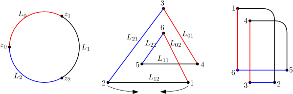
Figure 5. Generators for $\mathcal{M}_{J}(T_{\operatorname{id}},T_{1},T_{\operatorname{id}})$.

Next we show that $\#\mathcal{M}^{\chi}_{J}(T_{\operatorname{id}},T_{1},T_{\operatorname{id}})=0$, for $\chi\leq 2$. The generators are shown in Figure 5. As $d\to 0$, $\dot{F}^{\prime}_{(12)}$ bubbles off as a triangle $\{p_{1},p_{2},p_{a}\}$. Then $p_{a}$ should be mapped to the intersection of the extension of the line segments $(q^{\prime\prime}_{1}q^{\prime\prime}_{6})$ and $(q^{\prime\prime}_{2}q^{\prime\prime}_{3})$. But this is impossible since the degree of the projection $\pi_{T^{*}I_{2}}\circ u$ is 0 near the intersection. ∎

The similar arguments will be used in the proofs of Propositions 4.1 and 4.2. In general, $\dot{F}^{\prime}_{(12)}$ always bubbles off as a triangle as $d\to 0$. Here, $q^{\prime}_{1},q^{\prime}_{2}$ are on the bottom Lagrangian $L_{1\kappa}$ in the $T^{*}I_{1}$-direction. We then analyze the remaining irreducible components of $\dot{F}^{\prime}$ and reduce the problem to simpler cases.

Lemma 3.4.

$T_{1}\cdot T_{\operatorname{id}}=T_{1}$.

Proof.

This is similar to the proof of Lemma 3.3. ∎

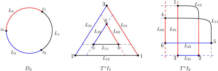
Figure 6. Generators for $\mathcal{M}_{J}(T_{1},T_{1},T_{\operatorname{id}})$.

Lemma 3.5.

$T_{1}\cdot T_{1}=T_{\operatorname{id}}+\hbar T_{1}$.

Proof.

We first show that

(3.3) $$\#\mathcal{M}^{\chi}_{J}(T_{1},T_{1},T_{\operatorname{id}})=\left\{\begin{array}[]{lr}1,\,\,\chi=2&\\ 0,\,\,\chi<2&\end{array}.\right.$$

The generators are shown in Figure 6.

If $\chi=2$, then there is a unique trivial holomorphic curve consisting of two disks, so $\#\mathcal{M}^{\chi=2}_{J}(T_{1},T_{1},T_{\operatorname{id}})=1$.

If $\chi<2$, then $\dot{F}^{\prime}_{(12)}$ bubbles off as a triangle as $d\to 0$. The projection of $\dot{F}^{\prime}_{(12)}$ under $\pi_{T^{*}I_{2}}\circ u$ is a homeomorphism to the triangle $\{q^{\prime\prime}_{1},q^{\prime\prime}_{2},q^{\prime\prime}_{3}\}$. Consequently, the projection of $\dot{F}^{\prime}_{(3)}$ under $\pi_{T^{*}I_{2}}\circ u$ is the constant map to $q^{\prime\prime}_{3}$. Since $\pi_{T^{*}I_{2}}\circ u$ is of degree 0 or 1 near $q^{\prime\prime}_{3}$, the image of $\pi_{T^{*}I_{2}}\circ u(\dot{F}\backslash(\dot{F}^{\prime}_{(12)}\cup\dot{F}^{\prime}_{(3)}))$ is disjoint from $q^{\prime\prime}_{3}$. It follows that $\dot{F}^{\prime}_{(12)}\cup\dot{F}^{\prime}_{(3)}$ is a connected component of $\dot{F}^{\prime}$. Therefore, $\dot{F}$ consists of two components before the degeneration, which are homeomorphically mapped to the triangles $\{q^{\prime\prime}_{1},q^{\prime\prime}_{2},q^{\prime\prime}_{3}\}$ and $\{q^{\prime\prime}_{4},q^{\prime\prime}_{5},q^{\prime\prime}_{6}\}$ under $\pi_{T^{*}I_{2}}\circ u$, respectively. So $\chi=2$, which is a contradiction.  

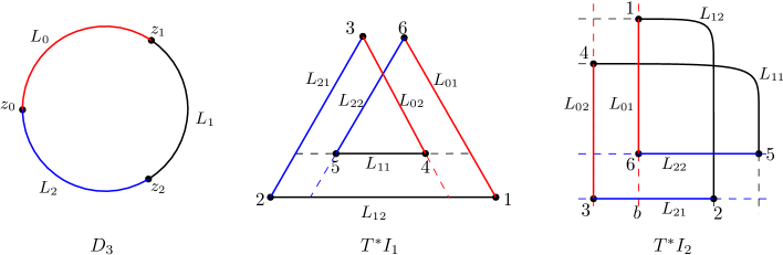
Figure 7. Generators for $\mathcal{M}_{J}(T_{1},T_{1},T_{1})$.

Figure 8. A disk $\dot{F}=D_{6}$ which satisfies the involution condition.

We next show that

(3.4) $$\#\mathcal{M}^{\chi}_{J}(T_{1},T_{1},T_{1})=\left\{\begin{array}[]{lr}1,\,\,\chi=1&\\ 0,\,\,\chi\neq 1&\end{array}.\right.$$

The generators are shown in Figure 7.

We denote the moduli space of domain $(\dot{F},j)$ by $\mathcal{M}(\dot{F})$. By Riemann-Roch formula, $\mathrm{dim}\,\mathcal{M}(\dot{F})=3(\kappa-\chi)$. Consider the moduli space of pseudoholomorphic maps from $(\dot{F},j)$ to each direction $D_{3}$, $T^{*}I_{1}$ and $T^{*}I_{2}$, denoted by $\mathcal{M}(D_{3})$, $\mathcal{M}({T^{*}I_{1}})$ and $\mathcal{M}({T^{*}I_{2}})$, respectively. The index formula says

$$\mathrm{dim}\,\mathcal{M}(D_{3})=\mathrm{dim}\,\mathcal{M}({T^{*}I_{1}})=\mathrm{dim}\,\mathcal{M}({T^{*}I_{2}})=2(\kappa-\chi),$$

for generic $J$. We have

(3.5) $$\mathcal{M}_{J}(T_{1},T_{1},T_{1})=\mathcal{M}(D_{3})\cap\mathcal{M}({T^{*}I_{1}})\cap\mathcal{M}({T^{*}I_{2}}),$$

This is our main strategy to count curves in $\mathcal{M}_{J}(T_{1},T_{1},T_{1})$: we compute the moduli space for each direction and then count their intersection number.

The moduli space of curves restricted to each direction has an explicit parametrization. For example, $\pi_{D_{3}}\circ u$ from $\dot{F}$ to $D_{3}$ is a $\kappa$-fold branched cover, and its restriction to $\partial\dot{F}$ is a $\kappa$-fold cover over $S^{1}$. Generically, $\pi_{D_{3}}\circ u$ is parametrized by the positions of $\kappa-\chi$ double branch points on $\dot{F}$ over $D_{3}$.

In the case $\kappa=2$ and $\chi=1$, $\dot{F}=D_{6}$ is a disk with 6 boundary punctures. The moduli space of $(\dot{F},j)$ is

$$\mathcal{M}(\dot{F})\simeq\mathbb{R}^{3}.$$

Then we consider the cut-out moduli space $\mathcal{M}(D_{3})$, viewed as a subset of $\mathcal{M}(\dot{F})$. The deck transformation of $\pi_{D_{3}}\circ u$ imposes an involution condition on $\dot{F}$. In other words, we require that $\{p_{i},p_{i+3}\}$ lie on a diameter for $i=1,2,3$ after some fractional linear transformation. Therefore,

$$\mathcal{M}(D_{3})\simeq\mathbb{R}^{2}.$$

The moduli spacce $\mathcal{M}(D_{3})$ admits a compactification $\overline{\mathcal{M}}(D_{3})$, which is described in Figure 9.

Figure 9. The compactified moduli space $\overline{\mathcal{M}}(D_{3})$ is described by the hexagon. Index $i$ stands for $p_{i}\in\partial\dot{F}$. The indices inside brackets describe the bubbling behavior, e.g., $(12)(45)$ means $p_{1}$ and $p_{2}$ (resp. $p_{4}$ and $p_{5}$) are close to each other. The involution condition is preserved on boundary strata, e.g., the cross ratio of the two bubble disks on the stratum $(123)(456)$ are the same.

We first consider $\partial\mathcal{M}(D_{3})\cap\mathcal{M}(T^{*}I_{1})$. The map from a disk to the middle of Figure 7 may have a double branch point inside the inner region with degree 2. As the branch point touches the boundary of the inner region, it is replaced by a slit with 2 switch points along the Lagrangians. Since we are interested in $\partial\mathcal{M}(D_{3})$, the bubbling behavior in Figure 9 requires the slit to be very long so that some switch point meets another Lagrangian. The involution condition further requires that such switch points come in pairs. We conclude that $\partial\mathcal{M}(D_{3})\cap\mathcal{M}(T^{*}I_{1})$ consists of two points : one passes $q^{\prime}_{5}$ to its left extending the line segment $(q^{\prime}_{4}q^{\prime}_{5})$ and downwards extending $(q^{\prime}_{6}q^{\prime}_{5})$; the other passes $p_{4}$ to its right extending $(q^{\prime}_{5}q^{\prime}_{4})$ and downwards extending $(q^{\prime}_{3}q^{\prime}_{4})$. The two points are decipted as the violet dots in Figure 10.

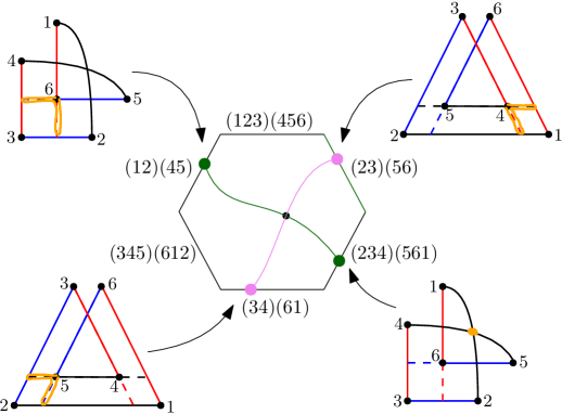
Figure 10. The orange curves in the pictures outside the hexagon represent slits. The black dot inside the hexagon is a curve in $\mathcal{M}_{J}(D_{3})\cap\mathcal{M}_{J}(T^{*}I_{1})\cap\mathcal{M}_{J}(T^{*}I_{2})$.

For $\partial\mathcal{M}(D_{3})\cap\mathcal{M}(T^{*}I_{2})$, consider the right of Figure 7. Similar to the previous paragraph, the degeneration of $D_{6}$ requires the existence of long slits. There are two curves: one with a slit passing $q^{\prime\prime}_{6}$ to its left and downwards; the other lies on the Lagrangian $(q^{\prime\prime}_{1}q^{\prime\prime}_{2})$ or $(q^{\prime\prime}_{4}q^{\prime\prime}_{5})$ with one switch point meeting the intersection point $(q^{\prime\prime}_{1}q^{\prime\prime}_{2})\cap(q^{\prime\prime}_{4}q^{\prime\prime}_{5})$. The two curves are decipted as the dark-green dots in Figure 10.

The violet and dark-green points in $\partial\mathcal{M}(D_{3})$ indicate that $\mathcal{M}(D_{3})\cap\mathcal{M}(T^{*}I_{1})$ and $\mathcal{M}(D_{3})\cap\mathcal{M}(T^{*}I_{2})$ have intersection of algebraic count 1 inside $\mathcal{M}(D_{3})$. Thus,

(3.6) $$\#\mathcal{M}^{\chi=1}_{J}(T_{1},T_{1},T_{1})=\#\mathcal{M}(D_{3})\cap\mathcal{M}(T^{*}I_{1})\cap\mathcal{M}(T^{*}I_{2})=1.$$

If $\chi\neq 1$, we show that $\#\mathcal{M}^{\chi}_{J}(T_{1},T_{1},T_{1})=0$. As $d\to 0$, $\dot{F}^{\prime}_{(12)}$ bubbles off as a triangle. Since the projection of $\dot{F}^{\prime}\backslash\dot{F}^{\prime}_{(12)}$ to $T^{*}I_{2}$ is of degree 1 to its image (the polygon composed of $\{q^{\prime\prime}_{3},q^{\prime\prime}_{4},q^{\prime\prime}_{5},q^{\prime\prime}_{6},q^{\prime\prime}_{b}\}$ in Figure 7), the domain before degeneration has to be a disk. This contradicts with the fact that $\chi\neq 1$. ∎

The counting in (3.6) is essentially the only case in our direct computation where a nontrivial curve exists. It corresponds to the deformation $\tilde{T}_{i}^{2}=1+\hbar\tilde{T}_{i}$ from the symmetric group to the Hecke algebra.

4. The general case

In this section, we compute $\operatorname{End}(L^{\otimes\kappa})$ by induction on $\kappa$. Recall that $\operatorname{End}(L^{\otimes\kappa})$ is freely generated by $T_{w}=\{y_{1},\cdots,y_{\kappa}\}$, where $y_{j}\in L_{0j}\cap L_{1w(j)}$ and $w\in S_{\kappa}$ is viewed as a permutation. We compute $T_{w_{1}}\cdot T_{w_{2}}$ for $w_{1},w_{2}\in S_{\kappa}$ by a case-by-case discussion depending on how $w_{1}$ acts on the last one or two elements of $\{1,\dots,\kappa\}$.

The first case is when $w_{1}$ fixes the last element. The schematic picture is shown in Figure 11. The following proposition is a generalization of Lemmas 3.2, 3.3.

Figure 11. The case for Proposition 4.1.

Proposition 4.1.

For $w_{1},w_{2},w_{3}\in S_{\kappa}$, suppose $w_{1}=w_{1}^{\prime},w_{2}=w_{2}^{\prime}s_{\kappa-1}s_{\kappa-2}\cdots s_{\kappa-m}$, where $w_{1}^{\prime},w_{2}^{\prime}\in S_{\kappa-1}$ and $m\geq 0$. We have

$$\#\mathcal{M}^{\chi}(T_{w_{1}},T_{w_{2}},T_{w_{3}})=\left\{\begin{array}[]{ll}\#\mathcal{M}^{\chi-1}(T_{w_{1}^{\prime}},T_{w_{2}^{\prime}},T_{w_{3}^{\prime}})&\mathrm{if}\,\,\,w_{3}=w_{3}^{\prime}s_{\kappa-1}s_{\kappa-2}\cdots s_{\kappa-m},\\ 0&\mathrm{otherwise},\end{array}\right.$$

where $w_{3}^{\prime}\in S_{\kappa-1}$.

Proof.

Suppose that the strand of $w_{3}$ starting from the position $\kappa$ ends on the position $t$. See the right of Figure 11. Here, we are reading the picture for $w_{3}$ from top to bottom. We consider the following three cases depending on $t$.

1. $t=\kappa-m$. Let $w_{3}=w_{3}^{\prime}s_{\kappa-1}s_{\kappa-2}\cdots s_{\kappa-m}$ for $w_{3}^{\prime}\in S_{\kappa-1}$. This case is shown in Figure 12. The last vertical strand of $w_{1}$ in Figure 11 corresponds to $p_{1}$ in Figure 12. As $d\to 0$, $\dot{F}^{\prime}_{(12)}$ bubbles off as a triangle with vertices $\{p_{1},p_{2},p_{a}\}$. The image of $\dot{F}^{\prime}_{(12)}$ in the $T^{*}I_{2}$-direction is the orange triangle and the image of $\dot{F}^{\prime}_{(3)}$ is the constant point $q^{\prime\prime}_{3}$. Since $\pi_{T^{*}I_{2}}\circ u$ is of degree 0 or 1 near $q^{\prime\prime}_{3}$, the image $\pi_{T^{*}I_{2}}\circ u(\dot{F}\backslash(\dot{F}^{\prime}_{(12)}\cup\dot{F}^{\prime}_{(3)}))$ is disjoint from $q^{\prime\prime}_{3}$. It implies that $\dot{F}^{\prime}_{(12)}\cup\dot{F}^{\prime}_{(3)}$ is a connected component of $\dot{F}^{\prime}$. Therefore, $\dot{F}_{(123)}$ is a connected component of $\dot{F}$ before the degeneration, and it is mapped homeomorphically to the triangle $\{q^{\prime\prime}_{1},q^{\prime\prime}_{2},q^{\prime\prime}_{3}\}$ under $\pi_{T^{*}I_{2}}\circ u$. After removing the component $\dot{F}_{(123)}$, we see that $\#\mathcal{M}^{\chi}(T_{w_{1}},T_{w_{2}},T_{w_{3}})=\#\mathcal{M}^{\chi-1}(T_{w^{\prime}_{1}},T_{w^{\prime}_{2}},T_{w^{\prime}_{3}})$.

   

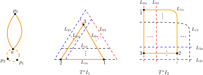
   Figure 12. The case $t=\kappa-m$.

2. $t>\kappa-m$. This case is shown in Figure 13. As $d\to 0$, $\dot{F}^{\prime}_{(12)}$ bubbles off as a triangle with vertices $\{p_{1},p_{2},p_{a}\}$. There is a vertex $p_{b}$ in the component $\dot{F}^{\prime}_{(3)}$ which is adjacent to $p_{a}$. Since $\pi_{T^{*}I_{2}}\circ u$ has degree 0 near the intersection between the extensions of $(q^{\prime\prime}_{1}q^{\prime\prime}_{b})$ and $(q^{\prime\prime}_{2}q^{\prime\prime}_{3})$, $\dot{F}^{\prime}_{(12)}$ cannot be a triangle. This leads to a contradiction. Therefore, $\#\mathcal{M}^{\chi}(T_{w_{1}},T_{w_{2}},T_{w_{3}})=0$.

   

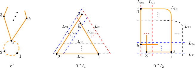
   Figure 13. The case $t>\kappa-m$.

3. $t<\kappa-m$. This case is shown in Figure 14. As $d\to 0$, $\dot{F}^{\prime}_{(12)}$ bubbles off as a triangle with vertices $\{p_{1},p_{2},p_{a}\}$. On one hand, similar to the proof of $\#\mathcal{M}_{J}(T_{\operatorname{id}},T_{\operatorname{id}},T_{1})=0$ of Lemma 3.2, the projection of $\dot{F}^{\prime}_{(b)}$ under $\pi_{D_{3}}\circ u$ is the constant map to $z_{0}$. On the other hand, the line denoted by the orange arrow is disjoint from $L_{0i}$ for $i=1,\dots,\kappa-1$ since $(q^{\prime}_{1}q^{\prime}_{b})$ lies on $L_{0\kappa}$. So $q^{\prime}_{b}$ cannot be separated from the bottom-left region. But the generators in this region are mapped to $z_{2}$ in the $D_{3}$-direction. We conclude that $\pi_{D_{3}}\circ u(\dot{F}^{\prime}_{(b)})$ cannot be far from $z_{2}$. This is a contradiction. Therefore, $\#\mathcal{M}^{\chi}(T_{w_{1}},T_{w_{2}},T_{w_{3}})=0$.

   

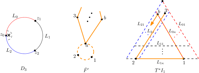
   Figure 14. The case $t<\kappa-m$.

This finishes the proof. ∎

The second case is when $w_{1}$ exchanges the last two elements. The schematic pictures are shown in Figures 15 and 16, which correspond to two subcases depending on the action of $w_{2}$ on the last two elements. The following proposition is a generalization of Lemmas 3.4, 3.5.

Figure 15. The case for Proposition 4.2 (1).

Figure 16. The case for Proposition 4.2 (2).

Proposition 4.2.

For $w_{1},w_{2},w_{3}\in S_{\kappa}$, suppose that $w_{1}=w_{1}^{\prime\prime}s_{\kappa-1}$, where $w_{1}^{\prime\prime}\in S_{\kappa-2}$.

1. If $w_{2}=w_{2}^{\prime\prime}s_{\kappa-2}\cdots s_{\kappa-m}s_{\kappa-1}s_{\kappa-2}\cdots s_{\kappa-l}$, where $w_{2}^{\prime\prime}\in S_{\kappa-2}$, $m>l\geq 0$, we have

   $$\#\mathcal{M}^{\chi}(T_{w_{1}},T_{w_{2}},T_{w_{3}})$$

   $$= \left\{\begin{array}[]{ll}\#\mathcal{M}^{\chi-2}(T_{w_{1}^{\prime\prime}},T_{w_{2}^{\prime\prime}},T_{w_{3}^{\prime\prime}})&\mathrm{if}\,\,\,w_{3}=w_{3}^{\prime\prime}s_{\kappa-1}s_{\kappa-2}\cdots s_{\kappa-m}s_{\kappa-1}s_{\kappa-2}\cdots s_{\kappa-l},\\ 0&\mathrm{otherwise},\end{array}\right.$$

   where $w_{3}^{\prime\prime}\in S_{\kappa-2}$.

2. If $w_{2}=w_{2}^{\prime\prime}s_{\kappa-1}s_{\kappa-2}\cdots s_{\kappa-m}s_{\kappa-1}s_{\kappa-2}\cdots s_{\kappa-l}$, where $w_{2}^{\prime\prime}\in S_{\kappa-2}$, $m>l\geq 0$, we have

   $$\#\mathcal{M}^{\chi}(T_{w_{1}},T_{w_{2}},T_{w_{3}})$$

   $$= \left\{\begin{array}[]{ll}\#\mathcal{M}^{\chi-2}(T_{w_{1}^{\prime\prime}},T_{w_{2}^{\prime\prime}},T_{w_{3}^{\prime\prime}})&\mathrm{if}\,\,\,w_{3}=w_{3}^{\prime\prime}s_{\kappa-2}\cdots s_{\kappa-m}s_{\kappa-1}s_{\kappa-2}\cdots s_{\kappa-l},\\ \#\mathcal{M}^{\chi-1}(T_{w_{1}^{\prime\prime}},T_{w_{2}^{\prime\prime}},T_{w_{3}^{\prime\prime}})&\mathrm{if}\,\,\,w_{3}=w_{3}^{\prime\prime}s_{\kappa-1}s_{\kappa-2}\cdots s_{\kappa-m}s_{\kappa-1}s_{\kappa-2}\cdots s_{\kappa-l},\\ 0&\mathrm{otherwise},\end{array}\right.$$

   where $w_{3}^{\prime\prime}\in S_{\kappa-2}$.

Proof.

The proof is similar to but slightly longer than that of Proposition 4.1 since we need to discuss the last two strands of $w_{1}$ instead of one. We keep track of the following labels.

• The strands of $w_{3}$ which start from the positions $\kappa$ and $\kappa-1$ end on positions $t_{1}$ and $t_{2}$, respectively.

• The strands of $w_{3}$ which end on the position $\kappa-m$ and $\kappa-l$ start from positions $r_{1}$ and $r_{2}$, respectively.

Figure 17 describes the part of generators $T_{w_{1}},T_{w_{2}}$ corresponding to the last two strands of $w_{1}$, where the dashed circles describe the undetermined $T_{w_{3}}$. We discuss Cases (1) and (2) separately in the following.

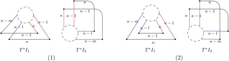
Figure 17. The part of generators $T_{w_{1}},T_{w_{2}}$ for Cases (1) and (2).

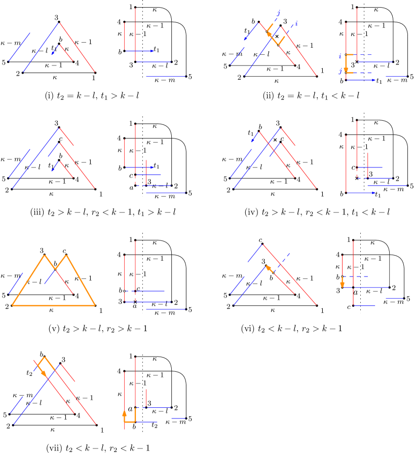
Figure 18. The subcases of Case (1).

(1) We first consider the case when $t_{1}=\kappa-m$, $t_{2}=\kappa-l$. This is equivalent to $w_{3}=w_{3}^{\prime\prime}s_{\kappa-1}s_{\kappa-2}\cdots s_{\kappa-m}s_{\kappa-1}s_{\kappa-2}\cdots s_{\kappa-l},$ for some $w_{3}^{\prime\prime}\in S_{\kappa-2}$. Consider a holomorphic curve in $\mathcal{M}^{\chi}(T_{w_{1}},T_{w_{2}},T_{w_{3}})$ which contains two trivial disks corresponding to the last two strands of $w_{1}$. The remaining components represent a curve in $\mathcal{M}^{\chi-2}(T_{w_{1}^{\prime\prime}},T_{w_{2}^{\prime\prime}},T_{w_{3}^{\prime\prime}})$. Thus, $\mathcal{M}^{\chi-2}(T_{w_{1}^{\prime\prime}},T_{w_{2}^{\prime\prime}},T_{w_{3}^{\prime\prime}})$ can be viewed as a subset of $\mathcal{M}^{\chi}(T_{w_{1}},T_{w_{2}},T_{w_{3}})$. We show that no other curve exists in the rest of the proof. The subcases are shown in Figure 18.

1. $t_{2}=k-l$, $t_{1}>k-l$. As $d\to 0$, $\dot{F}_{(12)}$ bubbles off as a triangle with vertices $\{p_{1},p_{2},p_{a}\}$, where $p_{a}\in\dot{F}^{\prime}$ is the nodal point mapped to the limit of $q_{1}^{\prime}$ and $q_{2}^{\prime}$ in the $T^{*}I_{1}$-direction. Then the projection of $\dot{F}^{\prime}_{(3)}$ to the $T^{*}I_{2}$-direction must be the constant map to $q_{3}^{\prime\prime}$. Since $\pi_{T^{*}I_{2}}\circ u$ is of degree 0 or 1 near $q_{3}$, the image $\pi_{T^{*}I_{2}}\circ u(\dot{F}\backslash(\dot{F}^{\prime}_{(12)}\cup\dot{F}^{\prime}_{(3)}))$ is disjoint from $q^{\prime\prime}_{3}$. It implies that $\dot{F}^{\prime}_{(12)}\cup\dot{F}^{\prime}_{(3)}$ is a connected component of $\dot{F}^{\prime}$. Therefore, the triangle $\{p_{1},p_{2},p_{3}\}$ forms a connected component of $\dot{F}$ before the degeneration. By removing the triangle $\{p_{1},p_{2},p_{3}\}$, the problem reduces to the case (2) of Proposition 4.1 with $\kappa-1$-strands. Hence, $\#\mathcal{M}^{\chi}(T_{w_{1}},T_{w_{2}},T_{w_{3}})=0$.

2. $t_{2}=k-l$, $t_{1}<k-l$. As $d\to 0$, $\dot{F}_{(12)}$ bubbles off as a triangle with vertices $\{p_{1},p_{2},p_{a}\}$ and the projection of $\dot{F}^{\prime}_{(3)}$ to the $T^{*}I_{2}$-direction must be the constant map to $q^{\prime\prime}_{3}$. Moreover $\dot{F}^{\prime}_{(3)}$ is a bigon with possible nodal degeneration points which are connected to other irreducible components of $\dot{F}^{\prime}$. Denote one of such nodal points on $\dot{F}^{\prime}$ by $p_{n}$, whose images in $T^{*}I_{1}$ and $T^{*}I_{2}$ are drawn as the crossings in Figure 18 (ii). We now remove the bigon $\dot{F}^{\prime}_{(3)}$ from $\dot{F}^{\prime}$ but keep $p_{n}$ remained. We denote the irreducible component containing $p_{n}$ in the remaining part of $\dot{F}^{\prime}$ by $\dot{F}^{\prime}_{p_{n}}$.

   In the $T^{*}I_{2}$-direction, the projection of $u(\dot{F}^{\prime}\backslash\dot{F}^{\prime}_{(3)})$ to the left side of the vertical dotted line is of degree 1. Let $C$ be the boundary of the image $\pi_{T^{*}I_{2}}\circ(\dot{F}^{\prime}_{p_{n}})$. Then the part of $C$ near $L_{0{\kappa}}\cap L_{2(\kappa-l)}$ is locally drawn as the orange lines, which goes from $L_{2i}$ to $L_{2j}$ on $L_{0\kappa}$ for $i>\kappa-l$, $j<\kappa-m$. We denote the preimage of the orange arrow from $L_{2i}$ to $L_{2j}$ by $C_{arrow}$. It has the positive boundary orientation.

   In the $T^{*}I_{1}$-direction, the position of the crossing must be above $L_{0\kappa}$ since $\pi_{D_{3}}\circ u(p_{n})=z_{0}$. However, the image of $C_{arrow}$, denoted by the orange arrow, has the negative boundary orientation. This leads to a contradiction. Therefore, $\#\mathcal{M}^{\chi}(T_{w_{1}},T_{w_{2}},T_{w_{3}})=0$.

3. $t_{2}>k-l$, $r_{2}<k-1$, $t_{1}>k-l$. As $d\to 0$, $\dot{F}_{(12)}$ bubbles off as a triangle with vertices $\{p_{1},p_{2},p_{a}\}$. Since on $T^{*}I_{2}$, $\pi_{T^{*}I_{2}}\circ u$ is of degree 0 near the intersection of the extension of $(q^{\prime\prime}_{1}q^{\prime\prime}_{c})$ and $(q^{\prime\prime}_{2}q^{\prime\prime}_{3})$, $\{p_{1},p_{2},p_{a}\}$ cannot form a triangle. This leads to a contradiction. Therefore, $\#\mathcal{M}^{\chi}(T_{w_{1}},T_{w_{2}},T_{w_{3}})=0$.

4. $t_{2}>k-l$, $r_{2}<k-1$, $t_{1}<k-l$. As $d\to 0$, $\dot{F}_{(12)}$ bubbles off as a triangle with vertices $\{p_{1},p_{2},p_{a}\}$, where $p_{a}$ is mapped to a point in $T^{*}I_{2}$, denoted by a crossing. We denote the preimage of this crossing in the irreducible component other than $\dot{F}_{(12)}$ and $\dot{F}_{(3)}$ by $p_{n}$. The image of $p_{n}$ in $T^{*}I_{1}$ is also denoted by a crossing. It sits above $L_{0\kappa}$ for the same reason as in (ii). The remaining argument is the same as in (ii). We conclude that $\#\mathcal{M}^{\chi}(T_{w_{1}},T_{w_{2}},T_{w_{3}})=0$.

5. $t_{2}>k-l$, $r_{2}>k-1$. As $d\to 0$, $\dot{F}_{(12)}$ bubbles off as a triangle $T$ with vertices $\{p_{1},p_{2},p_{a}\}$, where $p_{a}$ is mapped to the crossing in $T^{*}I_{2}$. The other irreducible component of $\dot{F}^{\prime}$ containing $p_{a}$ is the quadrilateral $Q$ with vertices $\{p_{3},p_{c},p_{a},p_{b}\}$ which is the bottom-left part in the $T^{*}I_{2}$-direction. Figure 19 describes the degenerated domain $\dot{F}^{\prime}$.

   Removing $T$ and $Q$ from $\dot{F}^{\prime}$ corresponds to removing the orange polygon in the $T^{*}I_{1}$-direction. As a result, the vertices $\{p_{1},p_{2},p_{3},p_{c}\}$ are replaced by $p_{b}$. Then the problem is reduced to the case (2) of Proposition 4.1 with $\kappa-1$ strands. Hence, $\#\mathcal{M}^{\chi}(T_{w_{1}},T_{w_{2}},T_{w_{3}})=0$.

   

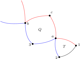
   Figure 19. The subcase (v).

6. $t_{2}<k-l$, $r_{2}>k-1$. This is similar to (ii). The orientation of the orange arrows leads to a contradiction. Hence $\#\mathcal{M}^{\chi}(T_{w_{1}},T_{w_{2}},T_{w_{3}})=0$.

7. $t_{2}<k-l$, $r_{2}<k-1$. This is similar to (ii). So $\#\mathcal{M}^{\chi}(T_{w_{1}},T_{w_{2}},T_{w_{3}})=0$.

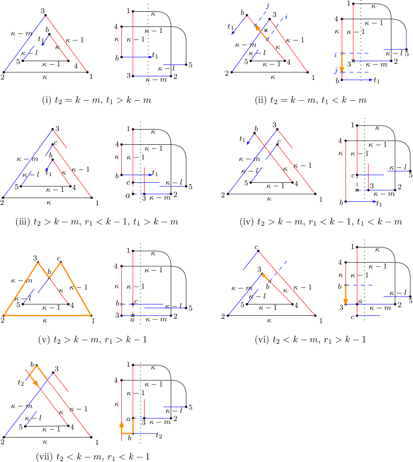
Figure 20. The subcases of Case (2).

(2) The subcases are shown in Figure 20. The proofs of all subcases are similar to those in (1) except for the subcase (v). We discuss the subcase (v) only and omit the others.

1. $t_{2}>k-m$, $r_{1}>k-1$. The proof is similar to that of the subcase (v) of (1). As $d\to 0$, $\dot{F}_{(12)}$ bubbles off as a triangle $T$ with vertices $\{p_{1},p_{2},p_{a}\}$, where $p_{a}$ is mapped to the crossing in $T^{*}I_{2}$, and $\{p_{3},p_{c},p_{a},p_{b}\}$ forms a quadrilateral $Q$, as the bottom-left part in the $T^{*}I_{2}$-direction. Figure 19 describes the degenerated domain $\dot{F}^{\prime}$. Removing $T$ and $Q$ from $\dot{F}^{\prime}$ corresponds to removing the orange polygon in the $T^{*}I_{1}$-direction. As a result, the vertices $\{p_{1},p_{2},p_{3},p_{c}\}$ are replaced by $p_{b}$. Then the problem is reduced to the case with $\kappa-1$ strands. There are three possibilities.

   1. $t_{2}=\kappa-l$. This is similar to the case (1) of Proposition 4.1. If the limiting curve exists, then $\{p_{1},p_{2},p_{3},p_{4},p_{5},p_{c}\}$ must forms a (hexagon) disk component $H$ of $\dot{F}$. The count of $u\in\mathcal{M}^{\chi}(T_{w_{1}},T_{w_{2}},T_{w_{3}})$ restricted to $H$ is exactly the count of $\mathcal{M}^{\chi=1}_{J}(T_{1},T_{1},T_{1})$ in Lemma 3.5, which is equals 1. The count of $u$ restricted to $\dot{F}\backslash H$ is the count of $\mathcal{M}^{\chi-1}(T_{w_{1}^{\prime\prime}},T_{w_{2}^{\prime\prime}},T_{w_{3}^{\prime\prime}})$. Therefore, $\#\mathcal{M}^{\chi}(T_{w_{1}},T_{w_{2}},T_{w_{3}})=\#\mathcal{M}^{\chi-1}(T_{w_{1}^{\prime\prime}},T_{w_{2}^{\prime\prime}},T_{w_{3}^{\prime\prime}})$.

   2. $t_{2}>\kappa-l$. This is similar to the case (2) of Proposition 4.1. So $\#\mathcal{M}^{\chi}(T_{w_{1}},T_{w_{2}},T_{w_{3}})=0$.

   3. $t_{2}<\kappa-l$. This is similar to the case (3) of Proposition 4.1. So $\#\mathcal{M}^{\chi}(T_{w_{1}},T_{w_{2}},T_{w_{3}})=0$.

This finishes the proof. ∎

The following corollaries are direct consequences by inductively using the two propositions above.

Corollary 4.3.

The generator $T_{{\operatorname{id}}}$ is the identity in $\operatorname{End}(L^{\otimes\kappa})$.

Corollary 4.4.

We have $T_{i}T_{w}=\left\{\begin{array}[]{ll}T_{s_{i}w}&\mathrm{if}\,\,\,l(s_{i}w)>l(w)+1,\\ T_{s_{i}w}+\hbar T_{w}&\mathrm{if}\,\,\,l(s_{i}w)<l(w)-1.\end{array}\right.$

Corollary 4.5.

The generators $T_{i}$ satisfy the relations in the Hecke algebra:

(4.1) $$T_{i}^{2} =1+\hbar T_{i},$$

(4.2) $$T_{i}T_{j} =T_{j}T_{i}\,\,\,\mathrm{for}\,\,\,|i-j|>1,$$

(4.3) $$T_{i}T_{i+1}T_{i} =T_{i+1}T_{i}T_{i+1}.$$

Proof of Theorem 1.2.

Define a unital $\mathbb{Z}[\hbar]$-algebra map $\phi:H_{\kappa}\to\operatorname{End}(L^{\otimes\kappa})$ on the algebra generators by $\phi(\tilde{T}_{i})=T_{i}$. The map is well-defined by Corollary 4.5. The multiplication rules on $H_{\kappa}$ in (1.3) and that of $\operatorname{End}(L^{\otimes\kappa})$ in Corollary 4.4 are the same. So we have $\phi(\tilde{T}_{w})=T_{w}$ for all $w\in S_{\kappa}$. ∎

References

- [Abo12] Mohammed Abouzaid “On the wrapped Fukaya category and based loops” In J. Symplectic Geom. 10.1, 2012, pp. 27–79 URL: http://projecteuclid.org/euclid.jsg/1332853049
- [AS10] Alberto Abbondandolo and Matthias Schwarz “Floer homology of cotangent bundles and the loop product” In Geom. Topol. 14.3, 2010, pp. 1569–1722 DOI: 10.2140/gt.2010.14.1569
- [CHT20] Vincent Colin, Ko Honda and Yin Tian “Applications of higher-dimensional Heegaard Floer homology to contact topology”, 2020 arXiv:2006.05701 [math.SG]
- [ES19] Tobias Ekholm and Vivek Shende “Skeins on branes”, 2019 arXiv:1901.08027 [math.SG]
- [GPS18] Sheel Ganatra, John Pardon and Vivek Shende “Sectorial descent for wrapped Fukaya categories”, 2018 arXiv:1809.03427
- [GPS20] Sheel Ganatra, John Pardon and Vivek Shende “Covariantly functorial wrapped Floer theory on Liouville sectors” In Publ. Math. Inst. Hautes Études Sci. 131, 2020, pp. 73–200 DOI: 10.1007/s10240-019-00112-x
- [HTY22] Ko Honda, Yin Tian and Tianyu Yuan “Higher-dimensional Heegaard Floer homology and Hecke algebras”, 2022 arXiv:2202.05593 [math.SG]
- [MS21] Hugh Morton and Peter Samuelson “DAHAs and skein theory” In Comm. Math. Phys. 385.3, 2021, pp. 1655–1693 DOI: 10.1007/s00220-021-04052-8
- [Syl19] Zachary Sylvan “On partially wrapped Fukaya categories” In J. Topol. 12.2, 2019, pp. 372–441 DOI: 10.1112/topo.12088