Three-dimensional tomographic imaging of the magnetization vector field using Fourier transform holography

Abstract

In recent years, interest in expanding from 2D to 3D systems has grown in the magnetism community, from exploring new geometries to broadening the knowledge on the magnetic textures present in thick samples, and with this arise the need for new characterization techniques, in particular tomographic imaging. Here, we present a new tomographic technique based on Fourier transform holography, a lensless imaging technique that uses a known reference in the sample to retrieve the object of interest from its diffraction pattern in one single step of calculation, overcoming the phase problem inherent to reciprocal-space-based techniques. Moreover, by exploiting the phase contrast instead of the absorption contrast, thicker samples can be investigated. We obtain a 3D full-vectorial image of a $800$ nm-thick extended Fe/Gd multilayer in a $5\,\upmu$m-diameter circular field of view with a resolution of approximately $80$ nm. The 3D image reveals worm-like domains with magnetization pointing mostly out of plane near the surface of the sample but that falls in-plane near the substrate. Since the FTH setup is fairly simple, it allows modifying the sample environment. Therefore, this technique could enable in particular a 3D view of the magnetic configuration’s response to an external magnetic field.

I Introduction

Three-dimensional magnetic textures have recently attracted increasing interest both from fundamental and a technological point of view  Streubel et al. (2016); Fernández-Pacheco et al. (2017); Fischer et al. (2020); Nguyen et al. (2015); May et al. (2019); Kent et al. (2021); Meng et al. (2021); Donnelly et al. (2021, 2022). This emergent field of research comes hand in hand with the need for new characterization techniques, in particular to obtain tomographic images of the magnetic textures. Among the wide variaty of magnetic microscopies, transmission based techniques offer the possibility to extend their capabilities to 3D, that is, to probe the magnetization as a vector field through the depths of the material. Such capability has been demonstrated for neutrons Manke et al. (2010); Hilger et al. (2018), x-rays Streubel et al. (2016); Donnelly et al. (2017) and electrons Wolf et al. (2019, 2022), at distinct length scales. The development done with neutrons allowed to image the magnetic domain distribution in the bulk, electrons permitted the characterization of the domain walls and observation of skyrmion tubes in objects of approximately $100$ nm thickness, whereas x-ray magnetic tomography allowed to observe new textures, such as Bloch points Donnelly et al. (2017), merons Hierro-Rodriguez et al. (2020) and vortex rings Donnelly et al. (2020a), in samples from $200$ nm thickness for soft x-rays up to $5\,\upmu$m using hard x-rays.

In particular, x-rays offer a range of microscopic and tomographic techniques well suited to the study of micron size samples with nanoscale resolution. The magnetic sensitivity is usually obtained by exploiting x-ray magnetic circular dichroism van der Laan and Figueroa (2014), i.e., an absorption contrast for opposite helicities of circular polarizations of the incident light. High-resolution 2D imaging is routinely achieved with x-ray microscopes based on zone-plate optics. When operated in imaging mode (transmission x-ray microscopy, TXM), the resolution is given by the outermost zone width of the zone plate, whereas for scanning mode (scanning transmission x-ray microscopy, STXM) it is possible to achieve a higher resolution since the latter is given by the beam size Fischer et al. (2006). Both full-field TXM and STXM have been successfully extended into magnetic tomography techniques Suzuki et al. (2018); Witte et al. (2020); Donnelly et al. (2022); Hierro-Rodriguez et al. (2020); Hermosa et al. .

Exploiting the coherence of the beam can in principle provide a higher resolution, but more interesting is that it provides a phase contrast in addition to the absorption contrast, which shall be referred to here as x-ray magnetic circular birefringence. This aspect is particularly appealing to investigate thick samples, since the magnetic phase contrast can remain sizable a few eV away from the absorption edge Donnelly et al. (2016), which in turn reduces the sample damage. Coherence-based imaging techniques Miao et al. (2015), such as coherent diffraction imaging (CDI), Fourier transform holography (FTH) Stroke (1965) and ptychography, are well-suited to obtain 3D structural images Chapman et al. (2006); Guehrs et al. (2012); Holler et al. (2017) and 2D magnetic images with nanometric resolution Turner et al. (2011); Eisebitt et al. (2004); Tripathi et al. (2011). However, among the latter three techniques, only ptychography has so far been adapted to obtain full tomographic magnetic images Donnelly et al. (2017, 2020b); Rana et al. . Here we propose to extend FTH capabilities to 3D magnetic imaging.

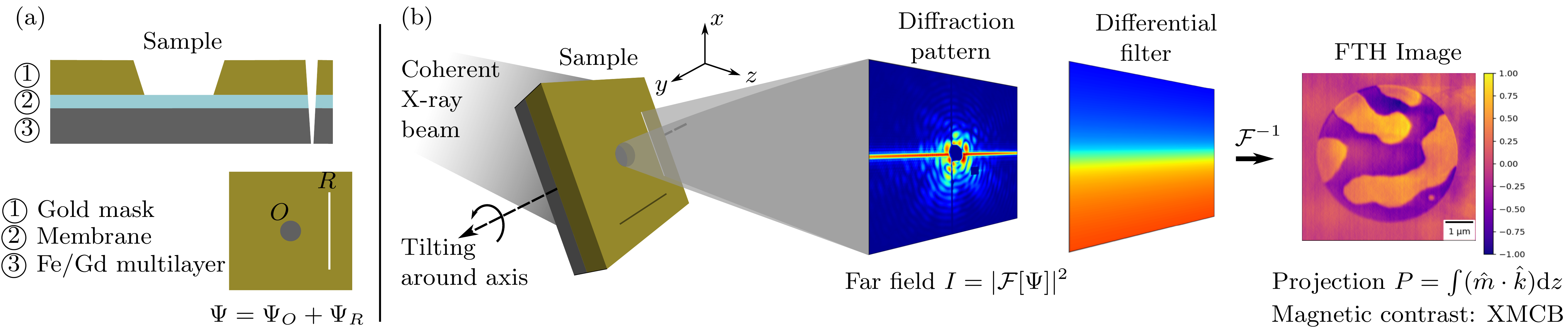
Figure 1: Magnetic nanotomography based on Fourier transform holography (FTH): (a) The sample for FTH has three layers – a gold mask, the membrane and the magnetic material of interest. (b) A circular window of $5\upmu$m-diameter is milled into the (opaque) gold layer, which coats the magnetic sample, to allow the x-rays to pass through. Two reference slits are also milled across the sample and coating. The coherent x-ray beam illuminates the whole sample. The complex x-ray amplitude after the sample, i.e., the exit wave, is denoted as $\Psi$. After filtering the reference from the diffraction pattern and applying an inverse Fourier transform, the magnetic projection is recovered. The magnetic contrast is obtained by x-ray magnetic circular birefringence (XMCB). Tilting the sample around axes $x$ and $y$ allows to probe all three components of the magnetization.

The main asset of Fourier Transform Holography Stroke (1965) is being able to retrieve an image of the structure from the experimental data in only one deterministic step. Moreover, it only requires a simple instrumental setup consisting of a pinhole to impose the high coherence of the incident beam, a rotating sample stage to select the magnetic projection and a beamstop – protecting the high resolution 2D detector in the far-field of the sample Popescu et al. (2019), which leaves space to implement the modification of the sample environment, such as controlling the temperature or applying an in situ magnetic field.

Indeed, the complexity resides mostly in the sample preparation. The required sample consists of the object of interest $O$ and a known reference $R$ (described in terms of 2D, complex transmission functions), which interfere in the coherent beam (see Fig. 1(a)). The holographic reconstruction provides an image which consists of the convolution of the object $O$ and the reference $R$. As a consequence, the resolution of FTH is limited by the reference size and quality. Additionally, phase retrieval algorithms can be used as a complementary method to improve the FTH resolution Flewett et al. (2012).

For extended references, following the HERALDO approach Guizar-Sicairos and Fienup (2007), a linear differential operator specific to the chosen reference can be exactly calculated and consecutively applied to the measured intensity. In this way, the real-space image is deconvoluted with the reference, so that a complex-valued image of the object can be retrieved in a single deterministic step (see Fig. 1(b)), rather than following an iterative approach. This image is equivalent to the object complex transmission coefficient if the object and the reference do not overlap Guizar-Sicairos and Fienup (2007).

FTH has shown to be useful to obtain 2D images of the magnetization in flat samples Duckworth et al. (2011, 2013); Turnbull et al. (2020); Birch et al. (2020). Its inherent mechanical stability thanks to the integration of the reference in the sample itself makes FTH particularly interesting for time-resolved measurements Wang et al. (2012); Bukin et al. (2016). In fact, what is measured in forward scattering is a projection of the magnetization, just as with any other transmission technique van der Laan (2008). This is the component of $\hat{m}$ that is parallel to the beam direction $\hat{k}$ integrated through the material along the said direction $r_{k}$:

$$P_{\hat{k}}=\int(\hat{m}\cdot\hat{k})\mathrm{d}r_{k}.$$ (1)

So whereas the first report of FTH focused on imaging the out-of-plane magnetization, i.e., the component perpendicular to the surface of the sample Eisebitt et al. (2004), if the sample is tilted the method also allows us to probe the in-plane magnetization components, using either a tilted reference hole Tieg et al. (2010) or an extended reference Duckworth et al. (2013). Furthermore, it has also been shown that it is possible to use FTH to perform tomography and obtain the 3D electronic density Guehrs et al. (2012, 2015).

In this work, we go further and use FTH as a 3D full-vectorial magnetic imaging technique. To this end, we tilt the sample around two orthogonal axes perpendicular to the beam direction and, for each tilt, we measure a dichroic projection image. Acquiring a dual set of dichroic projections has been proven using other techniques to be sufficient to reconstruct not only the charge density of an object but also all three components of the magnetization in an entire three-dimensional structureDonnelly et al. (2017, 2018); Hierro-Rodriguez et al. (2020), including the inner configuration.

This paper is structured as follows. In Sec. II, we describe the sample used to test the proposed technique, the experimental setup and we give the details regarding the data analysis. In Sec. III, we present a numerical validation of the method and analyze its limitations, followed by the experimental proof in Sec. IV. Finally, in Sec. V, we summarize the conclusions of this work.

II Experimental details

We test the proposed tomographic method experimentally on an Fe/Gd multilayer which displays worm-like magnetic domains with a typical width of $1$ $\upmu$m, as seen by magnetic force microscopy (MFM) (Fig. 2(a)). In-plane magnetization curves also show that, in spite of the dominating perpendicular magnetic anisotropy, it is expected to also have a persistent magnetic remanence as shown in the inset of Fig. 2(a). This coexistence of both in-plane and out-of-plane magnetization promises an intriguing 3D configuration, that cannot be mapped by 2D imaging techniques.

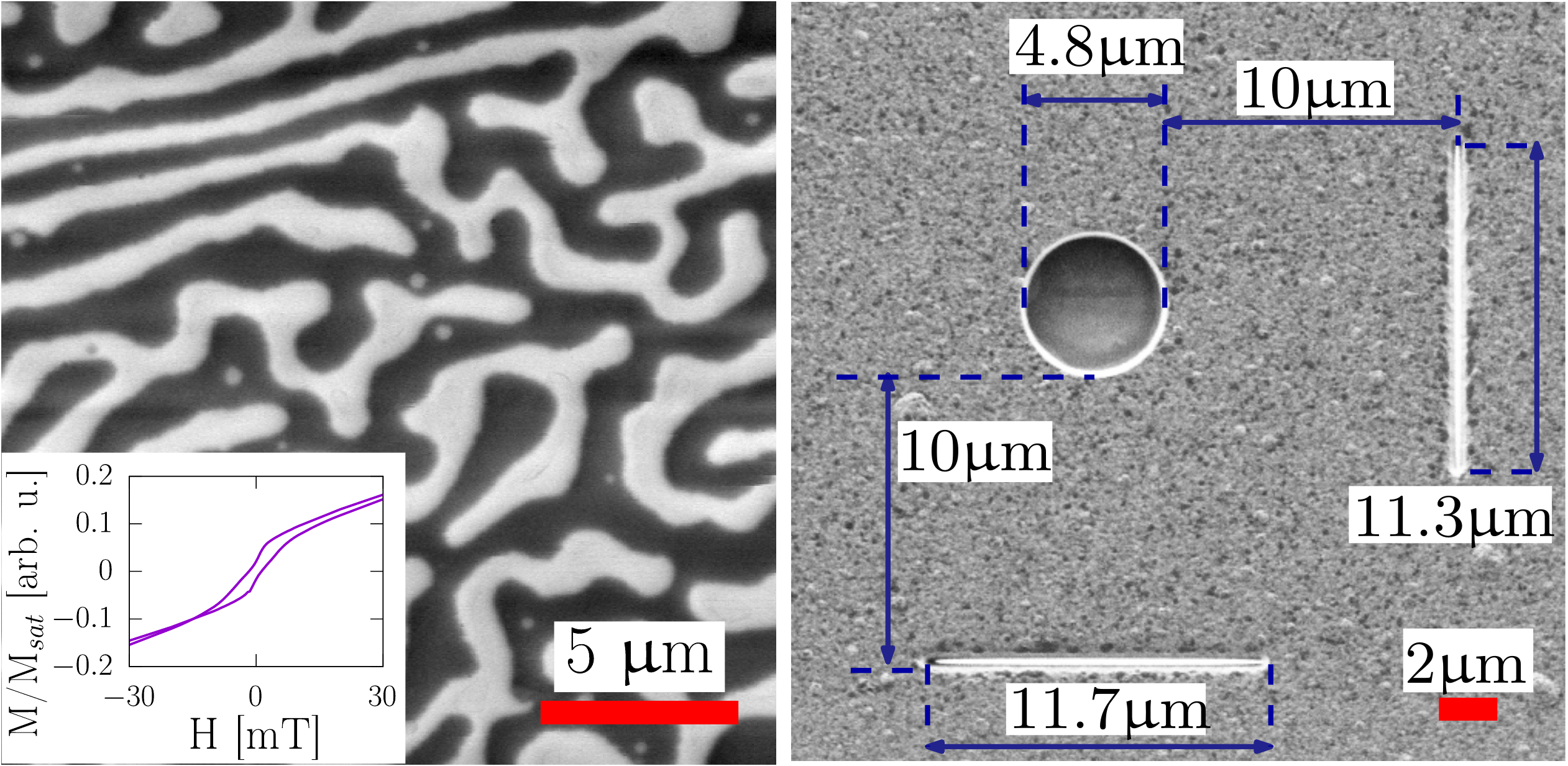
Figure 2: Details of the sample for 3D Fourier transform holography: (a) MFM image of the Fe/Gd multilayer grown on one side of a Si₃N₄ membrane. Inset: In-plane magnetic hysteresis loop. (b) SEM image of the Au mask grown on the other side of the membrane. A circular aperture and two reference slits are milled for doing 3D-FTH tomography.

The multilayer was sputtered at room temperature with deposition rates reaching $1.7$, $0.5$ and $1.2$ Å/sec for Ta, Fe and Gd, respectively, and limit pressure $7.10^{-8}$ mbar. The nominal stacking for this sample is Ta($6$)/[Fe($0.45$)/Gd($0.96$)]₆₀₀/Ta($6$) where the thicknesses are expressed in nm and $600$ is the number of repetitions of the bilayer. The average composition of this sample was measured with energy-dispersive x-ray spectroscopy (EDX) to be Fe_0.667Gd_0.333 and the total stack thickness as determined from scanning electron microscopy (SEM) is approximately $800$ nm.

The sample was grown on a $300$ nm-thick Si₃N₄ membrane suitable for x-ray measurements. This membrane was covered with a $1700$ nm-thick gold mask which is opaque to soft x-rays. The mask has also four $5$ nm-thick Ti layers grown intercalated with the Au to prevent the formation of large Au grains and the subsequent leakage of x-rays. Then we milled a circular aperture of diameter $d=5$ $\upmu$m into the gold mask using focused ion beam (FIB) to allow the transmission of x-rays. This aperture represents the object $O$ in the FTH approach (Fig. 1). To create the references $R$, two thin slits of length of $11\,\upmu$m, perpendicular to each other and at a distance $10\,\upmu$m of the circular aperture, were milled across the coating and the sample (Fig. 2(b)). The location and length of the slits meet the HERALDO separation conditions, which prevent the overlapping of the deconvoluted object and reference images Guizar-Sicairos and Fienup (2007). The width of the slits, which goes down to $\sim 80$ nm across the 2.8 $\mu$m total thickness of the full stack (see transversal slice of the slit in Fig. 1(a)), limits the resolution in one of the transverse directions in individual 2D images, while the resolution in the other transverse direction is limited to $\sim 50$ nm by the sharpness of the slit end.

The FTH data presented in this work was mainly acquired on the COMET endstation Popescu et al. (2019) at SEXTANTS beamline of SOLEIL synchrotron, and complementary data was measured at beamline ID32 of the ESRF. Both beamlines use similar setups. Circularly polarized x-rays are delivered by a helical undulator and the energy of the beam tuned by a grating monochromator. The coherence of the beam is ensured by a set of apertures in front of the endstation. The small angle coherent diffraction patterns are acquired on an area detector with a CCD camera (SEXTANTS), or a CMOS camera Desjardins et al. (2020) (ID32). The geometrical settings were such that the pixel size of the direct space images was $25$ nm at SEXTANTS and $50$ nm at ID32. To allow for tilting along two orthogonal axes, an azimuthal rotation of the sample holder was implemented, in addition to the existing tilt rotation. This setup is also compatible with the laminography geometry Witte et al. (2020).

To acquire the required dual set of projections, we tilt the sample around two orthogonal axes corresponding to the directions of both slits. By tilting around the $x$ axis according to Fig. 1, for example, the vertical slit is shadowed by the thickness of the sample, while the horizontal slit is not, hence the latter serves as the holographic reference for the measurements. In the same way, by tilting around the $y$ axis, the horizontal slit is now obscured and the vertical slit serves as the reference. Only close to normal incidence can both slits serve as a reference. We measured projections for $22$ tilt angles in total, getting $3$ images per polarization for each, with a total acquisition time of $130$ ms per image. The FTH measurements were performed at room temperature and at remanence.

The FTH images were reconstructed using a Python notebook based on the one provided in Ref. Birch et al. (2020), which in turn follows the HERALDO method Guizar-Sicairos and Fienup (2007). The FTH reconstruction algorithm provides complex-valued images, from which we extracted the phase since this quantity is proportional to the projection of the magnetization. To maximize the magnetic contrast of the images, we worked at $704.6$ eV, which is $2.1$ eV below the Fe $L_{3}$-edge. See the Appendix for more details on this.

Once all the measurements are processed and the set of projections is obtained, they are used as input for reconstructing the 3D magnetic configuration. To that end, we developed the PyCUDA library magtopy mag .

The reconstruction algorithm is based on the gradient descent method which has already been shown to be able to successfully reconstruct full-vectorial 3D magnetization configurations Donnelly et al. (2018). Starting with an initial guess for the 3D magnetic structure $\hat{m}_{0}(x,y,z)=\vec{0}$, the next update is directed by minimizing the error metric

$$\epsilon=\sum_{\phi}\sum_{x,y}\left(P^{(\phi)}(x,y)-P_{m}^{(\phi)}(x,y)\right)^{2},$$ (2)

where $\{P_{m}^{(\phi)}\}$ is the measured set of projections and $\{P^{(\phi)}\}$ is the one calculated from the guess as

$$P^{(\phi)}(x,y)=\sum_{z}R^{(\phi)}[\hat{m}]\cdot\hat{z}.$$ (3)

For each tilt angle $\phi$, the rotation matrix $R^{(\phi)}$ is applied to $\hat{m}$. Once the gradient $\frac{\partial\epsilon}{\partial\hat{m}}$ is calculated, the structure is updated according to

$$\hat{m}_{new}=\hat{m}-\alpha\frac{\partial\epsilon}{\partial\hat{m}}.$$ (4)

We included a step optimization according to which the best step $\alpha$ is estimated by imposing the condition

$$\epsilon_{k-1}-\epsilon_{k}>v,$$ (5)

so that the error decreases sufficiently in each step, that is, more than a certain value $v$.

It is worth noting that the chosen programming language for the library, PyCUDA, provides the interoperability of Python while taking advantage of high performance computing. The main algorithm is capable of reconstructing the 3D magnetic configuration of a $200^{3}$ voxels cube, or a ($5\,\upmu$m)³ cube considering a pixel size of $25$ nm, in one minute .

III Validation of the reconstruction algorithm

To validate the vectorial reconstruction of the magnetic configuration, as well as to understand its limitations, we considered one of the most relevant and common problems that can arise during the experiment, which is having a reduced angular range for the tomography, also known as missing wedge and addressed in Ref. Hierro-Rodriguez et al. (2018) with a different reconstruction algorithm. Another problem of FTH is the artifacts related to the imperfection of the references, for example an irregular slit end causes the overlay of weaker replicas over the main reconstruction. However, since these artifacts are bound to the sample fabrication stage, we will not address these in the present discussion.

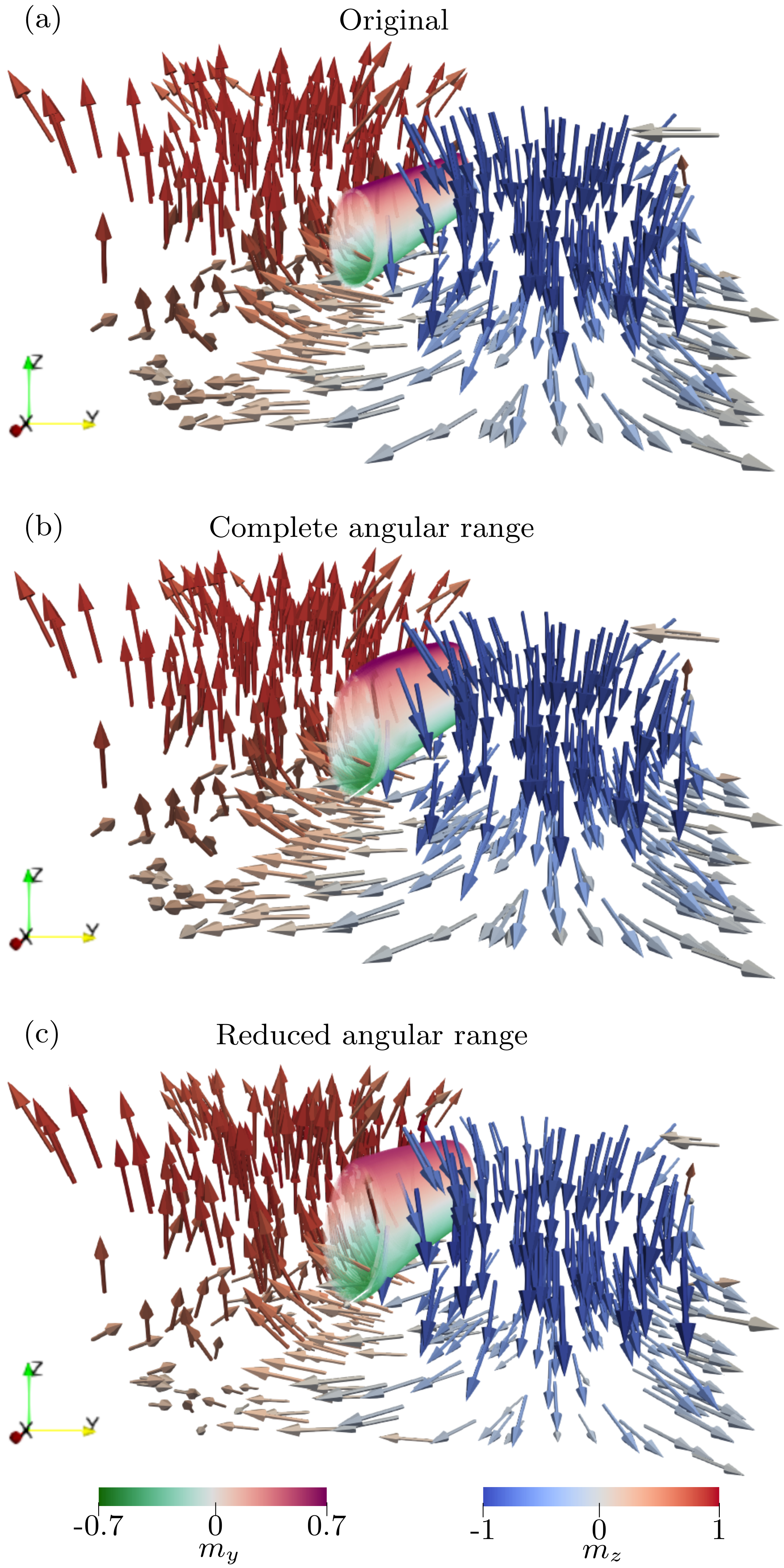
Figure 3: Comparison between the (a) original magnetic configuration from simulations and the reconstructed configurations from (b) a complete angular range which includes projections of the sample tilted from $-90$° to $90$°, and (c) the reduced angular range which only includes tilts from $-45$° to $45$°. Streamlines in the center of the structure highlight the core of the domain wall. The normalized reduced mean square error in each case is: (b) NRMSE$(m_{x})=3\%$, NRMSE$(m_{y})=2\%$, NRMSE$(m_{z})=2\%$ and (c) NRMSE$(m_{x})=24\%$, NRMSE$(m_{y})=5\%$, NRMSE$(m_{z})=5\%$.

We used as a test case the simulated magnetic configuration from Ref. Beutier et al. (2005) which has a size comparable to the experimental sample described above. The configuration, displayed in Fig. 3(a), shows two main domains with opposite out-of-plane (z-axis) magnetization and a domain wall with a Bloch-type core and two opposite Néel closure caps. The streamlines shown in the center of the structure highlight the position of the Bloch core.

Measuring several projections tilting the sample around $180$° leads to highly accurate reconstructions of the magnetic configuration, as can be seen in Fig. 3(b). There we can observe only a slight deformation of the streamlines in the domain wall core. The normalized reduced mean squared error (NRMSE ) calculated in this case is smaller than $3$% for all three components of the magnetization.

However, the accessible angular range is usually limited experimentally, for instance by the geometrical constraints of the setup, and in particular by the geometry of the supporting membrane and its frame, which may shadow the object of interest at shallow incidence angles. Therefore, we simulated projections for tilting angles ranging from $-45$° to $45$° to match the accessible ones in the experiment. The magnetic configuration reconstructed from the latter set is shown in Fig. 3(c).

We observe that the NRMSE of one of the in-plane components, $m_{x}$, increases to $24$%. The increased error is mainly due to the missing wedge effect. In particular, the magnetization along $x$ in this simulated system has a different behavior through the thickness of the sample than the rest, i.e., there is a larger component near the substrate that is not present near the surface. Compare the magnetic vectors on the top of the structure with the ones from the bottom: the former point mainly in the $z$ direction, while the latter are significantly tilted towards $x$. The information on this inhomogeneity is lost when no projections are given between $45$° and $90$°. Nevertheless, the NRMSE of the other two components remains at $5$%. A similar effect has been observed also in simulated Py discs measured between $-55$° and $55$° and reconstructed with a different algorithm Hierro-Rodriguez et al. (2018). From the streamlines in the center of the structure, we can see in detail how the walls are affected. In particular for the Néel caps, we see that $m_{y}$ is weaker compared to the original.

Altogether, note that the main features in the structure, namely the two opposite domains and the domain wall are successfully recovered and fully recognizable, which grants the method a robustness against the angular limitation.

IV Experimental results

Now let us return to the experiments. In Fig. 4(a), we show the full three-dimensional reconstruction of the magnetization vector field for the $800$ nm-thick Fe/Gd multilayer described in Sec. II. Two kinds of domains appear: one with the magnetization pointing mainly towards the surface of the disk (in negative $z$ direction) and another with the magnetization pointing mainly away from it (in positive $z$ direction). The general aspect of the magnetic structure is consistent with the MFM images performed on a full film (Fig. 2(a)). More interesting is the depth structure, which 2D measurements cannot capture.

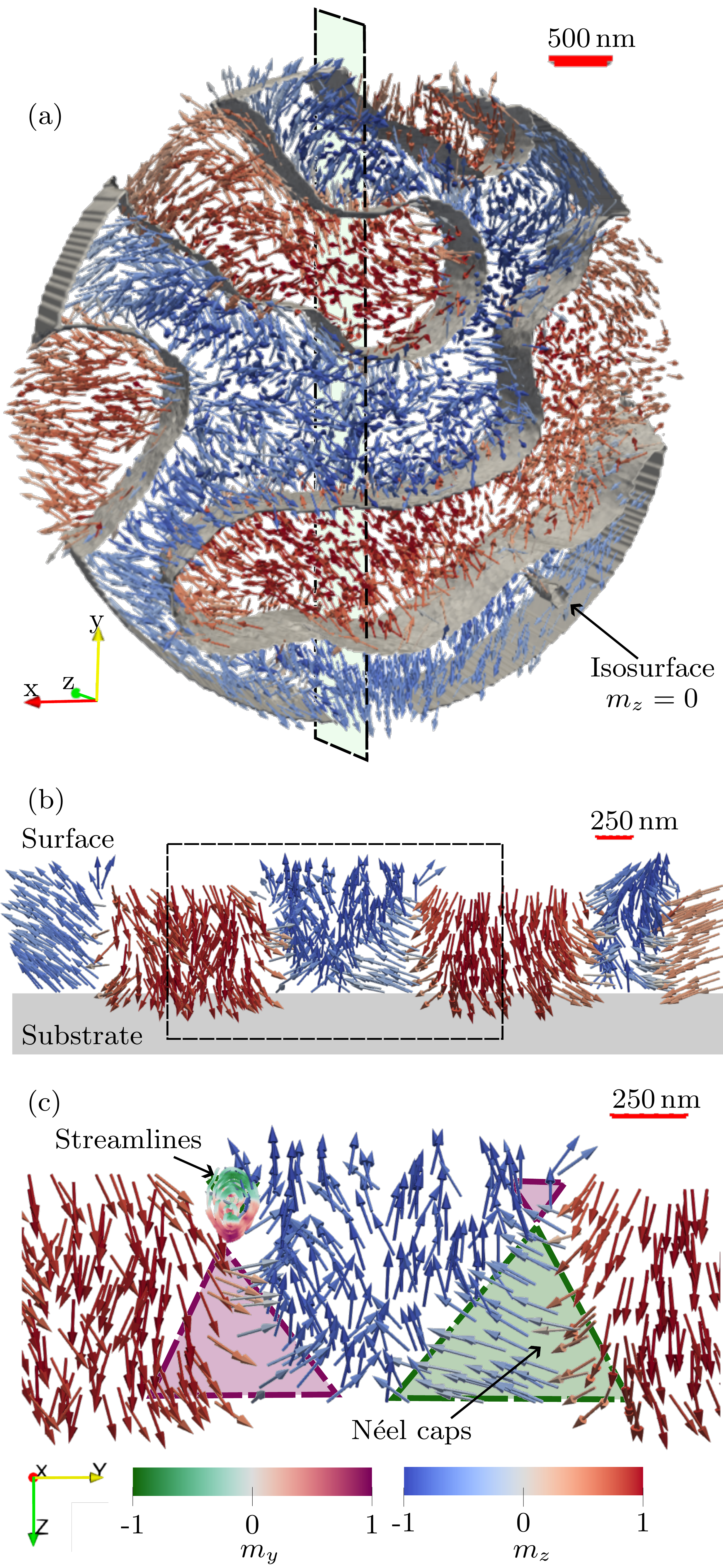
Figure 4: 3D magnetic image of the Fe/Gd multilayer obtained using Fourier transform holography with the two reference slit setup: (a) Overview of the magnetic vector field imaged through the circular aperture. In grey, the isosurface for $m_{z}=0$ hints mostly prismatic domains. The dashed rectangle indicates where the slice for (b) was taken, and in (b) the dashed rectangle indicates the area taken to show in more detail in (c). Both (b) and (c) have the same axes orientation.

The isosurface for $m_{z}=0$ is also displayed as an overlay in Fig. 4(a) and it shows the location of the walls that separate the two domains. From this we can observe that the shape of the domains as seen from the surface spans through the thickness, so that the isosurface appears perpendicular to the surface. In another words, the volume of each domain has a prismatic shape. In particular, a small tube, possibly a skyrmion, can also be spotted in the lower-right corner of the structure. Indeed, dipolar skyrmions have been reported in Fe/Gd multilayers Montoya et al. (2017) and seem to be present in the MFM measurement from Fig. 2(a) as well.

In Fig. 4(b), we present a transversal slice along the $y$ axis, through the middle of the sample, to show in detail the magnetization vector field. Here we observe that the in-plane component of the magnetization increases close to the substrate. In that area we can distinguish the Néel caps. Close to the borders we can notice the magnetization vector falling into the $y$ direction. This is an artifact that comes from the missing information of the borders for an extended system and it affects mostly an outer ring of approximately $500$ nm. This represents a limitation on the maximum field of view of the method used, that can be overcome by patterning a finite structure centered in the FTH aperture, as opposed to an extended one.

In Fig. 4(c), we show an area of the previous slice in more detail. Close to the top left corner, the streamlines help identifying the area of the Bloch core, similarly to the simulated system in Sec. III. The color code of the streamlines highlights that the upper area have negative $m_{y}$ whereas the bottom have positive $m_{y}$, corresponding to the two Néel caps. The colored triangles correspond to the area where $m_{y}>0.5$, and they represent the Néel caps. It can be observed that the Néel caps closer to the substrate are larger than the ones close to the surface. To estimate the width of the domain walls, we measured $m_{z}$ profile along $y$ in the first layer close to the surface ($z=0$ nm) and in the last layer near the substrate ($z=775$ nm), and we fitted a hyperbolic tangent. This will give us the domain wall width convoluted with the spatial resolution. We obtained a width of $100$ nm in the surface and $325$ nm near the substrate. If we do the same for the position of the core marked by the streamlines in Fig. 4(c) ($z=200$ nm), we obtain a width of $63$ nm.

The spatial resolution was estimated by calculating the Fourier shell correlation (FSC) pyn between two independent reconstructions. To this end, we split the projection set in two, and obtain a reconstruction configuration for each. We used the $1/2$-bit threshold criterion to ascertain the value of the spatial resolutionVan Heel and Schatz (2005). We show these curves in Fig. 5(a). The spatial resolution is $80$, $75$ and $60$ nm for each of the components of the magnetization: $m_{x}$, $m_{y}$ and $m_{z}$, respectively. These numbers are in-between the width of the slits ($\sim 80$ nm) and the sharpness of the slit ends, estimated to $\sim 50$ nm from individual 2D images. In particular, the resolution for $m_{z}$ matches the size of the Bloch core reported above. 2D FTH could achieve significantly higher resolution with a thinner and sharper reference ($17$ nm claimed in Ref. Turnbull et al. (2020)), which in turn would improve the resolution in the 3D reconstruction. For comparison, in previous soft x-rays dual-axis magnetic tomography based on transmission microscopy, a resolution of $85$ nm for a $400$ nm-thick film Hierro-Rodriguez et al. (2020) and $10$ nm for a $120$ nm-thick superlattice Rana et al. (2021) has been reported.

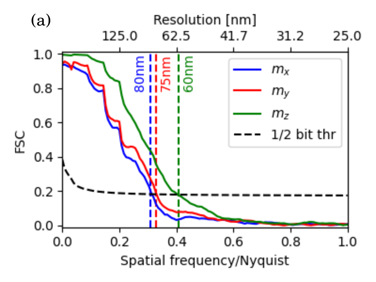
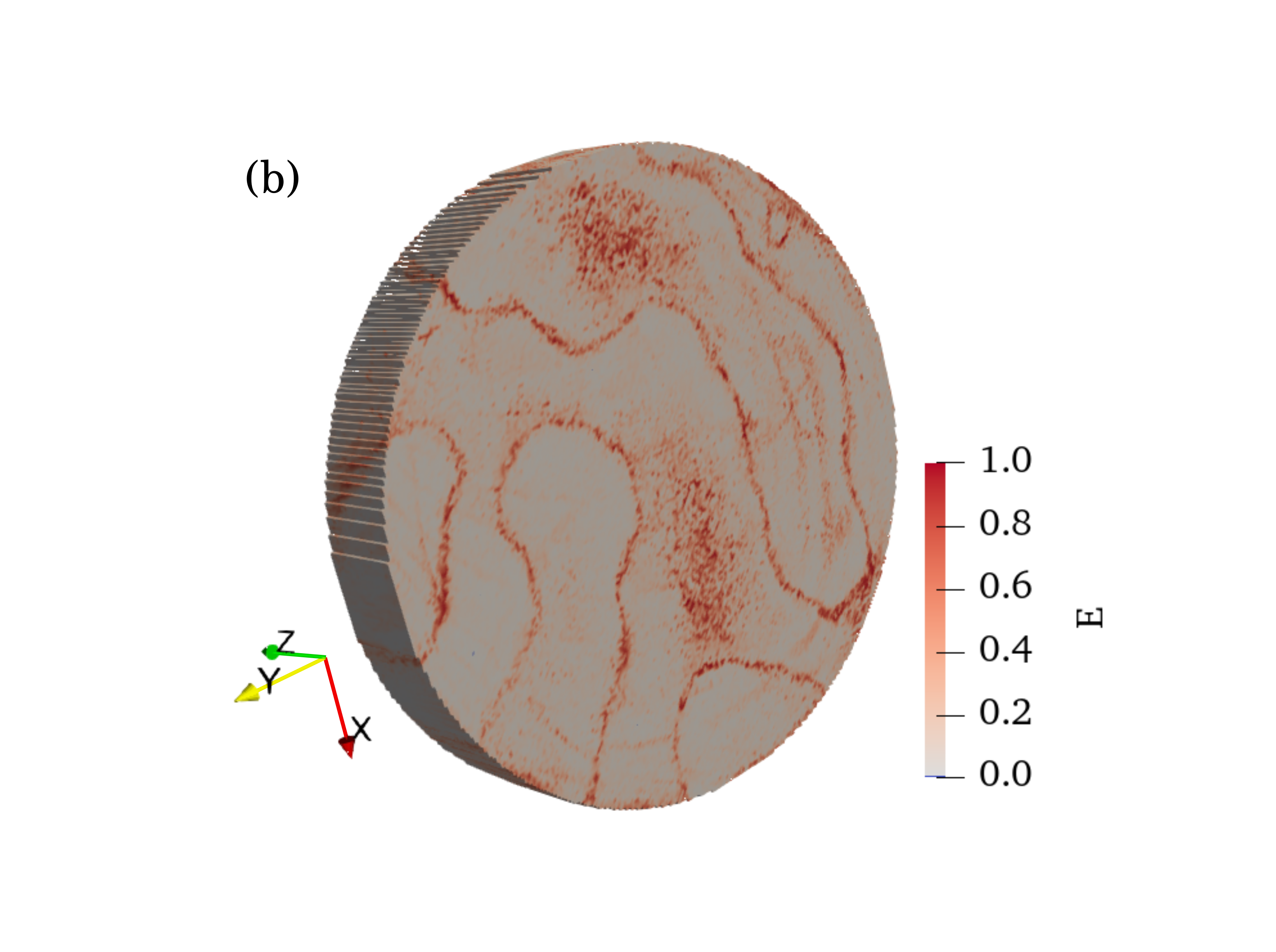
Figure 5: Spatial resolution and error in the 3D magnetic image of the Fe/Gd multilayer: (a) Spatial resolution estimated via Fourier Shell Correlation (FSC) for the three magnetization components. The $1/2$-bit threshold (dashed line) is used to estimate these values. (b) Error $E$ between the reconstructions acquired with two complementary projection sets. Only $1$% of the reconstruction has an error larger than 0.9 which means a complete opposite orientation of the magnetic moments. These are in turn concentrated in areas with artifacts coming from the FTH projection measurements and some specific regions of the domain walls.

While the FSC quantifies the resolution on average, to get a sense of the spatial localization of the error, we present also Fig. 5(b). Here, we show the error for each voxel of the reconstructed structure, defined as

$$\begin{split}&E=\\ &\frac{1}{2}\sqrt{(m_{x,1}-m_{x,2})^{2}+(m_{y,1}-m_{y,2})^{2}+(m_{z,1}-m_{z,2})^{2}},\end{split}$$ (6)

where the components with subscript $1$ and $2$ correspond to the two different projection sets used to calculate the FSC as described above. Note how the error is mainly concentrated approximately $75$ nm around the area of the domain walls as well as in specific regions of the domains. The latter can be directly related to FTH measurement artifacts previously observed in the projection images, and in the reconstruction, these affect the inner layers (larger $z$) the most, doubling its value for the layer closest to the substrate. Altogether, this shows that the 3D reconstruction concentrates its reliability in the domain area.

Magnetometry and MFM measurements can shed light on the observed phenomenon of in-plane magnetization predominance close to the substrate. We considered two other samples that are thinner than the one used for 3D-FTH. While the sample used in the 3D-FTH experiment has $N=600$ repetitions of [Fe($0.45$ nm)/Gd($0.96$ nm)], the other two have $150$ and $300$ repetitions of the same Fe/Gd bilayer, corresponding to a thickness of $200$ nm and $400$ nm, respectively. The hysteresis loops of these three, as well as MFM images of the surface of each sample at remanence, are shown in Fig. 6.

Extraordinary Hall effect (EHE) measurements provide sensitivity to the out-of-plane magnetization component. The thinnest sample’s ($200$ nm) EHE data reveals a square hysteresis loop indicating perpendicular anisotropy (Fig. 6(e)). With this in mind, we can understand its MFM image (Fig. 6(a)). The broad domains correspond to mostly up and down magnetization. The large size is the reason for the contrast being stronger close to the domain walls since a Néel character is expected close to the surface. This is expected for films that are thicker than the dipolar-exchange length like this one, since this allows for a better flux closure Hubert and Schäfer (1998).

The behavior of this $200$ nm-thick sample is however more complicated than a typical perpendicular system with only uniaxial anisotropy. Indeed, the in-plane magnetometry data shown in Fig. 6(d) features a clear hysteresis with sizeable remanence, as well as a large in-plane susceptibility up to significant values of $M/M_{\mathrm{s}}$. Both characteristics disappear at larger thicknesses i.e., for the $400$ and $800$ nm-thick multilayers, which indicates less favorable in-plane magnetization. In turn, MFM images show that the large domains give way to perpendicular stripe-like domains and eventually worm domains when the thickness increases (see Fig. 6(b) and (c)). When measuring thinner samples, the surface, to which the MFM is sensitive, is closer to the substrate, so we get more sensitive to any influence the substrate can have on the rest of the sample. Hence, this results hint at a decrease of the out-of-plane component near the substrate.

The Gd content has an specific effect on the sample behavior. Specifically, this sample effectively displays a ferrimagnetic behavior, such that the magnetic moments of Fe and Gd are antiferromagnetically coupled. This is observed by EHE measurements (Fig. 6.(d-e)) showing inverted loops. Indeed, at our average sample composition, the corresponding alloy’s magnetization is dominated by Gd Hansen et al. (1989), whereas the EHE is expected to be more sensitive to the perpendicular magnetization of Fe in this material McGuire et al. (1976), and since the Fe is antiferromagnetically aligned with the Gd, the magnetic loop is consequently expected to be inverted Bhatt et al. (2021); Stanciu et al. (2020); Becker et al. (2017); Stavrou and Röll (1999).

It has previously been observed that in transition-metal-Gd thin films, the Gd may segregate towards the surfaces Kim et al. (2019) where oxidation can occur Bergeard et al. (2017). Aside from oxidation, a loss in Gd moment has also been reported for decreasing CoGd thickness in Ir/CoGd/Pt multilayers Streubel et al. (2018), suggesting a detrimental role of the interfaces with the transition-metal-Gd alloy. These material-specific phenomena, in addition to the more generic trend towards flux closure in thick films, add plausibility to distinct magnetic behaviors close to the sample surfaces compared to its bulk.

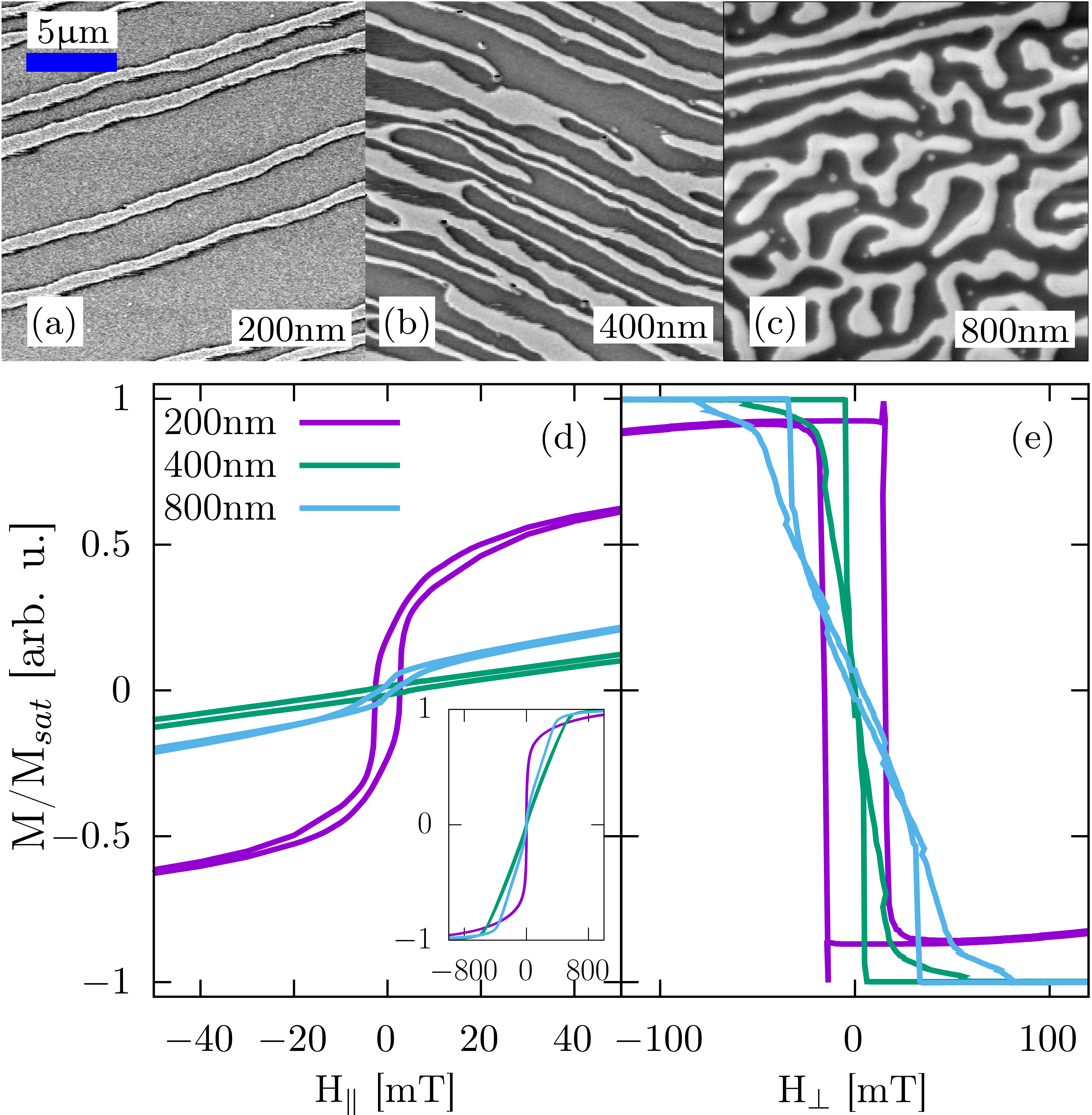
Figure 6: Magnetic behavior of Fe/Gd multilayers with different film thicknesses given by the total amount of bilayers stacked in each case: MFM images in remanence for $200$ (a), $400$ (b) and $800$ nm (c) of Fe/Gd; in-plane (d) and out-of-plane (e) hysteresis loops for the same three samples.

V Conclusions

We presented the first full-vectorial magnetic tomography based on Fourier transform holography achieving a resolution of $80$, $75$ and $60$ nm in $m_{x}$, $m_{y}$ and $m_{z}$, respectively. To that end, we used a sample with two slits as holographic references which allowed us to probe all three components of the magnetization within the sample.

We acquired the magnetic projections by deconvoluting the object from these references. The recovered image is complex-valued and, in particular, its phase is proportional to the magnetic projection. Measuring the phase at the pre Fe $L_{3}$-edge also allows us for high contrast in soft x-rays even in a $800$ nm-thick sample.

To validate our reconstruction method, we studied the effect of having a reduced angular range for tilting the sample and found that the missing wedge does not affect the recovering the out-of-plane magnetization nor the domain walls but it can fail recovering strong magnetic inhomogeneities or small domain caps.

To avoid reconstruction artifacts due to the missing information in the borders, we propose to use in the future patterned (finite) systems when utilizing FTH tomography with the dual-axis setup. For extended samples, the laminography setup represents a promising alternative since the information in the border of the disc is not lost. A future challenge will be to implement the aforementioned setup for FTH.

The resolution of the measurement is currently limited by the width of the reference and the sharpness of its ends, while the 3D reconstruction does not degrade it. It could in principle be significantly higher than demonstrated here, as 2D FTH images can be achieved down to 17 nm resolution at $3d$ transition metal $L$ edges Turnbull et al. (2020).

Magnetic tomography by FTH can take advantage of the fairly simple FTH setups, which allow large and various sample environments. It could for instance be performed under applied magnetic field using a multi-coil rotatable magnetic field Popescu et al. (2019) opening up the study of the either static or even dynamic response of the 3D magnetic configuration to this stimulus.

Appendix A

In a well conceived FTH experiment, the Fourier transform of the scattered intensity $g(\textbf{r})$ measured in the far field provides the convolution between the exit wave from the sample $\Psi(\textbf{r})$ and its inverse: $g(\textbf{r})=\Psi(\textbf{r})\star\Psi(\textbf{-r})$. The exit wave can be considered as the sum over the exit wave from the object of interest $\Psi_{O}(\textbf{r})$ and the exit wave from the reference $\Psi_{R}(\textbf{r})$. A region of interest in $g(\textbf{r})$ provides one of the cross-terms between object and reference: $\Psi_{O}(\textbf{r})\star\Psi_{R}(\textbf{r})$. For the sake of simplicity, we assume in the following that the reference wave is a Dirac function, such that we consider the extracted term as the exit wave from the object $\Psi_{O}(\textbf{r})$. The HERALDO approach with an infinitely sharp slit, which is the one we use in this paper, yields the same result after the application of a linear filter Guizar-Sicairos and Fienup (2007).

The exit wave results from the propagation through the sample of the incident wave. Assuming an incident flat wave, the exit wave can be expressed as

$$\Psi(x,y)=\exp\left(\frac{2\pi i}{\lambda}\int n\mathrm{d}z\right),$$ (7)

where $\lambda$ is the wavelength, $n$ is the optical index, the integration is along the beam axis $z$ and $x$ and $y$ are the transverse coordinates. The optical index includes a magnetic part, which will be detailed below.

In many published works using FTH, the real part of $\Psi(x,y)$ is used, since it has shown to give good qualitative images for the magnetization Eisebitt et al. (2004); Streit-Nierobisch et al. (2009); Turnbull et al. (2020); Birch et al. (2020); Duckworth et al. (2011, 2013). However, in order to perform tomography, a quantitative set of projections is needed. These are images that provide a quantity directly proportional to the magnetization of the sample. In that case, we notice that the real part actually consists in a mix between the absorption and refraction effects, both with magnetic components. Therefore, we take the phase instead, which includes only refraction effects. The phase of $\Psi(x,y)$ is

$$\Phi(x,y)=\frac{2\pi}{\lambda}\int n^{\prime}\mathrm{d}z,$$ (8)

where $n^{\prime}$ is the real part of the optical index. Eq. (8) remains correct as long as the phase spans over less than 2$\pi$.

Next we will detail the magnetic dependence of the optical index and its circular dichroism. The optical index reads:

$$n=1-\frac{r_{e}\lambda^{2}}{2\pi}\rho f,$$ (9)

where $r_{e}$ is the classical electron radius, $\rho$ the density of scatterers and $f$ their atomic scattering factor. At an absorption edge of the scatterers, when the incident beam is circularly polarised, the atomic scattering factor can be written as

$$f=f_{c}\pm f_{m}\hat{m}\cdot\hat{k},$$ (10)

where $f_{c}$ corresponds to the electron density factor, $f_{m}$ to the dichroic scattering factor and $\hat{m}\cdot\hat{k}$ is the magnetization component along the beam direction Hannon et al. (1988); van der Laan (2008). $f_{c}$ and $f_{m}$ are resonant spectroscopic terms with generally both real and imaginary parts, i.e., $f_{m}=f^{\prime}_{m}+if^{\prime\prime}_{m}$. The sign of the magnetic term in Eq. (10) changes with the helicity of the circular polarization. We point out that in the following, we will consider only the (resonant) scattering factors of iron. The contributions of Gd to magnetic scattering are negligible in our case, since we are measuring several hundreds of eV away from any absorption edge of Gd.

Combining Eqs. (8), (9) and (10), and assuming $\rho f_{m}$ constant (i.e., assuming the chemical homogeneity of the sample), we obtain the circular dichroism applied to the phase $\Phi(x,y)$ of the FTH reconstruction:

$$\Delta\Phi(x,y)=-r_{e}\lambda\rho f_{m}^{\prime}\int\hat{m}\cdot\hat{k}\mathrm{d}z$$ (11)

We see that the dichroic phase shift is proportional to the integrated projection onto the beam axis.

As mentioned above, Eq. (8) is valid a long as the phase shift spans over less than 2$\pi$, otherwise phase wraps will appear. If we assume the chemical homogeneity of the sample, the problem applies only to the dichroic part. According to Eq. (11), in the case of saturated magnetization along the beam direction, the phase shift is

$$\Delta\Phi=-r_{e}\lambda\rho f_{m}^{\prime}d$$ (12)

where $d$ is the thickness of the magnetic material. In the sample studied here, the total Fe thickness is around 255 nm, which corresponds to a phase shift around $\sim$0.6 rad at the energy of the measurement, well below the absorption edge (Figs. 7 and 8).

In contrast, the absorbance at the same energy is much lower, such that the absorption contrast would be very poor. At the peak of the magnetic absorbance, the phase contrast would vanish and the absorption contrast would be highest Donnelly et al. (2016), but the dependence of the absorption contrast on the magnetization is only approximately linear, for a sufficiently optically thin sample. The same holds for the real part, which is then the main reason why using it to calculate quantitatively the magnetization projection is only valid for thin samples.

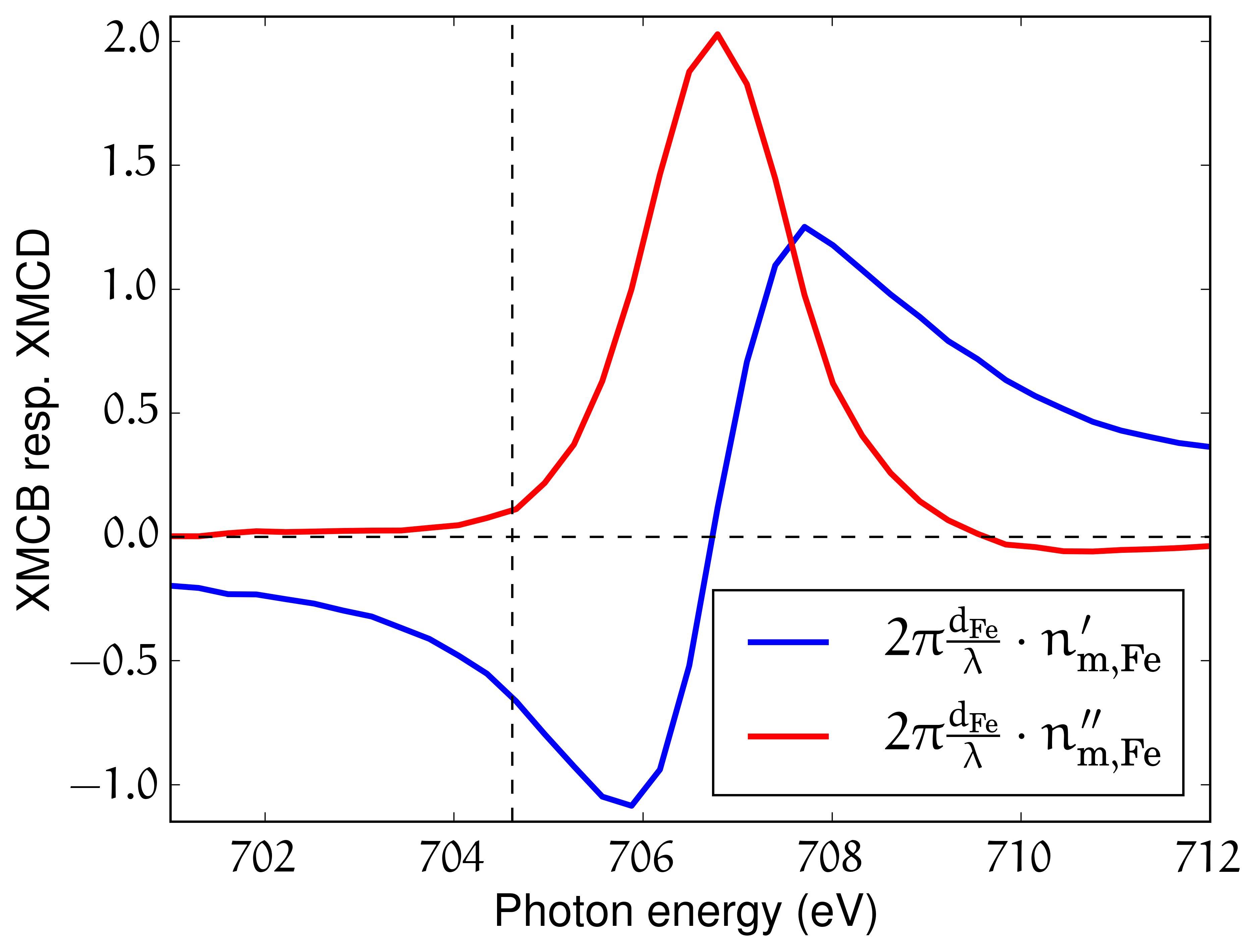
Figure 7: Calculated phase shift $\Delta\Phi=2\pi n^{\prime}_{\mathrm{m,Fe}}d_{\mathrm{Fe}}/\lambda$ and absorbance $2\pi n^{\prime\prime}_{\mathrm{m,Fe}}d_{\mathrm{Fe}}/\lambda$ induced by the magnetization in the Fe/Gd multilayer for a positive photon helicity, assuming saturated magnetization along the beam. The total Fe thickness is $d_{\mathrm{Fe}}=$255 nm. The real $n^{\prime}_{\mathrm{m,Fe}}$ and imaginary $n^{\prime\prime}_{\mathrm{m,Fe}}$ parts of the resonant magnetic contributions to the refractive index derive from the atomic scattering factor using $n_{\mathrm{m,Fe}}=-\frac{r_{\mathrm{e}}\lambda^{2}}{2\pi}\rho_{\mathrm{Fe}}f_{\mathrm{m,Fe}}$; the latter was taken from the measurements by Chen et al. Chen et al. (1995). At the used photon energy, we find a phase shift of -0.649 rad, and an absorbance of 0.107.

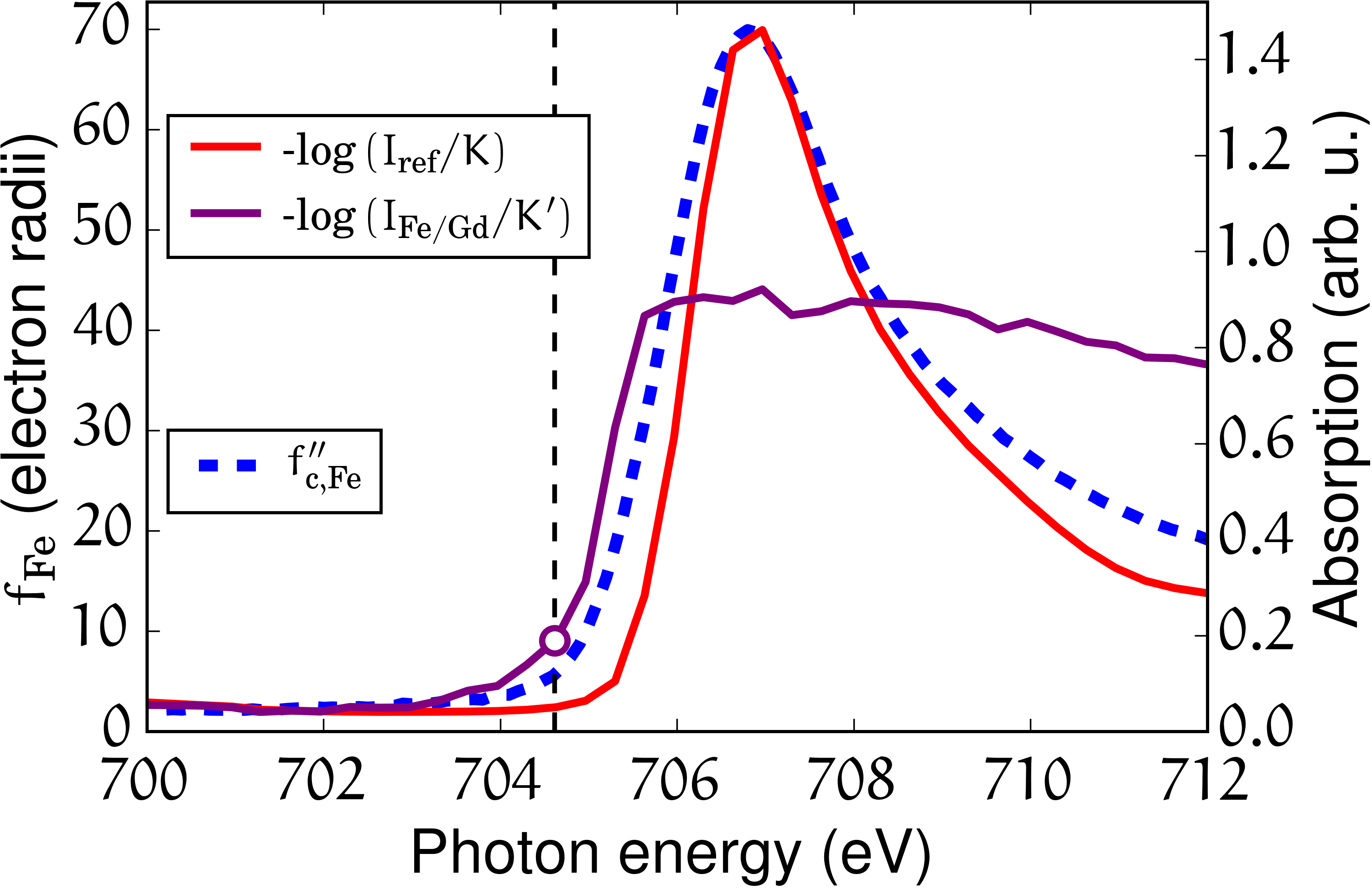
Figure 8: Spectroscopic data pertaining to Fe (dashed blue line) and transmission measurements on a reference Fe filter as well as our Fe/Gd multilayer (full lines, $K$ and $K^{\prime}$ are arbitrary normalization constants). The imaginary part of the atomic scattering factor Chen et al. (1995) related to the charge ($f^{\prime\prime}_{\mathrm{c,Fe}}$, blue dashed line) and the intensity transmitted through a thin Fe film (red full curve) were used to remove the small energy offset ($\sim 1$ eV) between the data obtained by Chen et al. and the measurements from SEXTANTS. The photon energy we used, $\sim 2.1$ eV below the peak of absorption, is indicated by the vertical dashed line. It lies at the onset of the measured transmission through the multilayer, and yet corresponds to the best signal-to-noise ratio we obtained with FTH.

References

- Streubel et al. (2016) R. Streubel, P. Fischer, F. Kronast, V. P. Kravchuk, D. D. Sheka, Y. Gaididei, O. G. Schmidt, and D. Makarov, Journal of Physics D: Applied Physics 49, 363001 (2016).
- Fernández-Pacheco et al. (2017) A. Fernández-Pacheco, R. Streubel, O. Fruchart, R. Hertel, P. Fischer, and R. P. Cowburn, Nature communications 8, 1 (2017).
- Fischer et al. (2020) P. Fischer, D. Sanz-Hernández, R. Streubel, and A. Fernández-Pacheco, APL Materials 8, 010701 (2020).
- Nguyen et al. (2015) V. Nguyen, O. Fruchart, S. Pizzini, J. Vogel, J.-C. Toussaint, and N. Rougemaille, Scientific reports 5, 1 (2015).
- May et al. (2019) A. May, M. Hunt, A. Van Den Berg, A. Hejazi, and S. Ladak, Communications Physics 2, 1 (2019).
- Kent et al. (2021) N. Kent, N. Reynolds, D. Raftrey, I. T. Campbell, S. Virasawmy, S. Dhuey, R. V. Chopdekar, A. Hierro-Rodriguez, A. Sorrentino, E. Pereiro, et al., Nature communications 12, 1 (2021).
- Meng et al. (2021) F. Meng, C. Donnelly, L. Skoric, A. Hierro-Rodriguez, J.-w. Liao, and A. Fernández-Pacheco, Micromachines 12, 859 (2021).
- Donnelly et al. (2021) C. Donnelly, K. L. Metlov, V. Scagnoli, M. Guizar-Sicairos, M. Holler, N. S. Bingham, J. Raabe, L. J. Heyderman, N. R. Cooper, and S. Gliga, Nature Physics 17, 316 (2021).
- Donnelly et al. (2022) C. Donnelly, A. Hierro-Rodríguez, C. Abert, K. Witte, L. Skoric, D. Sanz-Hernández, S. Finizio, F. Meng, S. McVitie, J. Raabe, et al., Nature nanotechnology 17, 136 (2022).
- Manke et al. (2010) I. Manke, N. Kardjilov, R. Schäfer, A. Hilger, M. Strobl, M. Dawson, C. Grünzweig, G. Behr, M. Hentschel, C. David, et al., Nature communications 1, 1 (2010).
- Hilger et al. (2018) A. Hilger, I. Manke, N. Kardjilov, M. Osenberg, H. Markötter, and J. Banhart, Nature communications 9, 1 (2018).
- Donnelly et al. (2017) C. Donnelly, M. Guizar-Sicairos, V. Scagnoli, S. Gliga, M. Holler, J. Raabe, and L. J. Heyderman, Nature 547, 328 (2017).
- Wolf et al. (2019) D. Wolf, N. Biziere, S. Sturm, D. Reyes, T. Wade, T. Niermann, J. Krehl, B. Warot-Fonrose, B. Büchner, E. Snoeck, et al., Communications Physics 2, 1 (2019).
- Wolf et al. (2022) D. Wolf, S. Schneider, U. K. Rößler, A. Kovács, M. Schmidt, R. E. Dunin-Borkowski, B. Büchner, B. Rellinghaus, and A. Lubk, Nature nanotechnology 17, 250 (2022).
- Hierro-Rodriguez et al. (2020) A. Hierro-Rodriguez, C. Quirós, A. Sorrentino, L. M. Álvarez-Prado, J. Martín, J. M. Alameda, S. McVitie, E. Pereiro, M. Velez, and S. Ferrer, Nature communications 11, 1 (2020).
- Donnelly et al. (2020a) C. Donnelly, S. Finizio, S. Gliga, M. Holler, A. Hrabec, M. Odstrčil, S. Mayr, V. Scagnoli, L. J. Heyderman, M. Guizar-Sicairos, et al., Nature nanotechnology 15, 356 (2020a).
- van der Laan and Figueroa (2014) G. van der Laan and A. I. Figueroa, Coordination Chemistry Reviews 277–228, 95 (2014).
- Fischer et al. (2006) P. Fischer, D.-H. Kim, W. Chao, J. A. Liddle, E. H. Anderson, and D. T. Attwood, Materials Today 9, 26 (2006).
- Suzuki et al. (2018) M. Suzuki, K.-J. Kim, S. Kim, H. Yoshikawa, T. Tono, K. T. Yamada, T. Taniguchi, H. Mizuno, K. Oda, M. Ishibashi, et al., Applied Physics Express 11, 036601 (2018).
- Witte et al. (2020) K. Witte, A. Späth, S. Finizio, C. Donnelly, B. Watts, B. Sarafimov, M. Odstrcil, M. Guizar-Sicairos, M. Holler, R. H. Fink, et al., Nano letters 20, 1305 (2020).
- (21) J. Hermosa, A. Hierro-Rodriguez, C. Quirós, J. I. Martin, A. Sorrentino, L. Aballe, E. Pereiro, M. Vélez, and S. Ferrer, 10.48550/arXiv.2206.02499.
- Donnelly et al. (2016) C. Donnelly, V. Scagnoli, M. Guizar-Sicairos, M. Holler, F. Wilhelm, F. Guillou, A. Rogalev, C. Detlefs, A. Menzel, J. Raabe, and L. J. Heyderman, Phys. Rev. B 94, 064421 (2016).
- Miao et al. (2015) J. Miao, T. Ishikawa, I. K. Robinson, and M. M. Murnane, Science 348, 530 (2015).
- Stroke (1965) G. W. Stroke, Applied Physics Letters 6, 201 (1965).
- Chapman et al. (2006) H. N. Chapman, A. Barty, S. Marchesini, A. Noy, S. P. Hau-Riege, C. Cui, M. R. Howells, R. Rosen, H. He, J. C. H. Spence, U. Weierstall, T. Beetz, C. Jacobsen, and D. Shapiro, J. Opt. Soc. Am. A 23, 1179 (2006).
- Guehrs et al. (2012) E. Guehrs, A. M. Stadler, S. Flewett, S. Frömmel, J. Geilhufe, B. Pfau, T. Rander, S. Schaffert, G. Büldt, and S. Eisebitt, New journal of physics 14, 013022 (2012).
- Holler et al. (2017) M. Holler, M. Guizar-Sicairos, E. H. Tsai, R. Dinapoli, E. Müller, O. Bunk, J. Raabe, and G. Aeppli, Nature 543, 402 (2017).
- Turner et al. (2011) J. J. Turner, X. Huang, O. Krupin, K. A. Seu, D. Parks, S. Kevan, E. Lima, K. Kisslinger, I. McNulty, R. Gambino, S. Mangin, S. Roy, and P. Fischer, Phys. Rev. Lett. 107, 033904 (2011).
- Eisebitt et al. (2004) S. Eisebitt, J. Lüning, W. Schlotter, M. Lörgen, O. Hellwig, W. Eberhardt, and J. Stöhr, Nature 432, 885 (2004).
- Tripathi et al. (2011) A. Tripathi, J. Mohanty, S. H. Dietze, O. G. Shpyrko, E. Shipton, E. E. Fullerton, S. S. Kim, and I. McNulty, Proceedings of the National Academy of Sciences 108, 13393 (2011), https://www.pnas.org/doi/pdf/10.1073/pnas.1104304108 .
- Donnelly et al. (2020b) C. Donnelly, S. Finizio, S. Gliga, M. Holler, A. Hrabec, M. Odstrčil, S. Mayr, V. Scagnoli, L. J. Heyderman, M. Guizar-Sicairos, et al., Nature Nanotechnology 15, 356 (2020b).
- (32) A. Rana, C.-T. Liao, E. Iacocca, J. Zou, M. Pham, E.-E. C. Subramanian, Y. H. Lo, S. A. Ryan, X. Lu, C. S. Bevis, R. M. K. Jr, A. J. Glaid, Y.-S. Yu, P. Mahale, D. A. Shapiro, S. Yazdi, T. E. Mallouk, S. J. Osher, H. C. Kapteyn, V. H. Crespi, J. V. Badding, Y. Tserkovnyak, M. M. Murnane, and J. Miao, 10.48550/arXiv.2104.12933.
- Popescu et al. (2019) H. Popescu, J. Perron, B. Pilette, R. Vacheresse, V. Pinty, R. Gaudemer, M. Sacchi, R. Delaunay, F. Fortuna, K. Medjoubi, et al., Journal of Synchrotron Radiation 26, 280 (2019).
- Flewett et al. (2012) S. Flewett, C. Günther, C. von Korff Schmising, B. Pfau, J. Mohanty, F. Büttner, M. Riemeier, M. Hantschmann, M. Kläui, and S. Eisebitt, Optics express 20, 29210 (2012).
- Guizar-Sicairos and Fienup (2007) M. Guizar-Sicairos and J. R. Fienup, Optics express 15, 17592 (2007).
- Duckworth et al. (2011) T. A. Duckworth, F. Ogrin, S. S. Dhesi, S. Langridge, A. Whiteside, T. Moore, G. Beutier, and G. van der Laan, Optics Express 19, 16223 (2011).
- Duckworth et al. (2013) T. A. Duckworth, F. Y. Ogrin, G. Beutier, S. S. Dhesi, S. A. Cavill, S. Langridge, A. Whiteside, T. Moore, M. Dupraz, F. Yakhou, et al., New Journal of Physics 15, 023045 (2013).
- Turnbull et al. (2020) L. A. Turnbull, M. T. Birch, A. Laurenson, N. Bukin, E. O. Burgos-Parra, H. Popescu, M. N. Wilson, A. Stefančič, G. Balakrishnan, F. Y. Ogrin, et al., ACS nano 15, 387 (2020).
- Birch et al. (2020) M. Birch, D. Cortés-Ortuño, L. Turnbull, M. Wilson, F. Groß, N. Träger, A. Laurenson, N. Bukin, S. Moody, M. Weigand, et al., Nature communications 11, 1 (2020).
- Wang et al. (2012) T. Wang, D. Zhu, B. Wu, C. Graves, S. Schaffert, T. Rander, L. Müller, B. Vodungbo, C. Baumier, D. P. Bernstein, B. Bräuer, V. Cros, S. de Jong, R. Delaunay, A. Fognini, R. Kukreja, S. Lee, V. López-Flores, J. Mohanty, B. Pfau, H. Popescu, M. Sacchi, A. B. Sardinha, F. Sirotti, P. Zeitoun, M. Messerschmidt, J. J. Turner, W. F. Schlotter, O. Hellwig, R. Mattana, N. Jaouen, F. Fortuna, Y. Acremann, C. Gutt, H. A. Dürr, E. Beaurepaire, C. Boeglin, S. Eisebitt, G. Grübel, J. Lüning, J. Stöhr, and A. O. Scherz, Phys. Rev. Lett. 108, 267403 (2012).
- Bukin et al. (2016) N. Bukin, C. McKeever, E. Burgos-Parra, P. Keatley, R. Hicken, F. Ogrin, G. Beutier, M. Dupraz, H. Popescu, N. Jaouen, et al., Scientific reports 6, 1 (2016).
- van der Laan (2008) G. van der Laan, Comptes Rendus Physique 9, 570 (2008).
- Tieg et al. (2010) C. Tieg, R. Frömter, D. Stickler, S. Hankemeier, A. Kobs, S. Streit-Nierobisch, C. Gutt, G. Grübel, and H. Oepen, Optics express 18, 27251 (2010).
- Guehrs et al. (2015) E. Guehrs, M. Fohler, S. Frömmel, C. M. Günther, P. Hessing, M. Schneider, L. Shemilt, and S. Eisebitt, New Journal of Physics 17, 103042 (2015).
- Donnelly et al. (2018) C. Donnelly, S. Gliga, V. Scagnoli, M. Holler, J. Raabe, L. J. Heyderman, and M. Guizar-Sicairos, New Journal of Physics 20, 083009 (2018).
- Note (1) MFM images were acquired at room temperature (RT) and zero field with a low-moment PPP-LM-MFMR tip from Nanosensors, monitoring the resonance frequency shift during the 2nd pass at a lift height of nm.
- Desjardins et al. (2020) K. Desjardins, K. Medjoubi, M. Sacchi, H. Popescu, R. Gaudemer, R. Belkhou, S. Stanescu, S. Swaraj, A. Besson, J. Vijayakumar, et al., Journal of Synchrotron Radiation 27, 1577 (2020).
- (48) Magtopy is a PyCUDA library that aims at the reconstruction of the 3D magnetization using as input a set of projections from tomography measurements. https://gitlab.com/magtopy/magtopy.
- Note (2) We measured a speed-up of in a GeForce RTX 3090 compared to the serial version of the code run in a CPU.
- Hierro-Rodriguez et al. (2018) A. Hierro-Rodriguez, D. Gürsoy, C. Phatak, C. Quirós, A. Sorrentino, L. M. Álvarez-Prado, M. Vélez, J. I. Martín, J. M. Alameda, E. Pereiro, et al., Journal of Synchrotron Radiation 25, 1144 (2018).
- Beutier et al. (2005) G. Beutier, G. van der Laan, K. Chesnel, A. Marty, M. Belakhovsky, S. Collins, E. Dudzik, J.-C. Toussaint, and B. Gilles, Physical Review B 71, 184436 (2005).
-
Note (3)
The normalized reduced mean squared error is defined as
follows,
where and are the reconstructed and the original 3D configuration, respectively, and is the size of the structure. - Montoya et al. (2017) S. Montoya, S. Couture, J. Chess, J. Lee, N. Kent, D. Henze, S. Sinha, M.-Y. Im, S. Kevan, P. Fischer, et al., Physical Review B 95, 024415 (2017).
- (54) We used the Fourier Shell Correlation function from PyNX http://ftp.esrf.fr/pub/scisoft/PyNX/.
- Van Heel and Schatz (2005) M. Van Heel and M. Schatz, Journal of structural biology 151, 250 (2005).
- Rana et al. (2021) A. Rana, C.-T. Liao, E. Iacocca, J. Zou, M. Pham, E.-E. C. Subramanian, Y. H. Lo, S. A. Ryan, X. Lu, C. S. Bevis, et al., arXiv preprint arXiv:2104.12933 (2021).
- Note (4) The multilayers for magnetometry and MFM investigations were grown on a Si/SiO2(1000Å) substrate.
- Hubert and Schäfer (1998) A. Hubert and R. Schäfer, Magnetic Domains: The Analysis of Magnetic Microstructures (Springer, 1998).
- Hansen et al. (1989) P. Hansen, C. Clausen, G. Much, M. Rosenkranz, and K. Witter, Journal of Applied Physics 66, 756 (1989).
- McGuire et al. (1976) T. R. McGuire, R. C. Taylor, and R. J. Gambino, in AIP Conference Proceedings (American Institute of Physics, 1976).
- Bhatt et al. (2021) R. C. Bhatt, L.-X. Ye, N. T. Hai, J.-C. Wu, and T.-h. Wu, Journal of Magnetism and Magnetic Materials 537, 168196 (2021).
- Stanciu et al. (2020) A. Stanciu, G. Schinteie, A. Kuncser, N. Iacob, L. Trupina, I. Ionita, O. Crisan, and V. Kuncser, Journal of Magnetism and Magnetic Materials 498, 166173 (2020).
- Becker et al. (2017) J. Becker, A. Tsukamoto, A. Kirilyuk, J. Maan, T. Rasing, P. Christianen, and A. Kimel, Physical Review Letters 118, 117203 (2017).
- Stavrou and Röll (1999) E. Stavrou and K. Röll, Journal of applied physics 85, 5971 (1999).
- Kim et al. (2019) D.-H. Kim, M. Haruta, H.-W. Ko, G. Go, H.-J. Park, T. Nishimura, D.-Y. Kim, T. Okuno, Y. Hirata, Y. Futakawa, H. Yoshikawa, W. Ham, S. Kim, H. Kurata, A. Tsukamoto, Y. Shiota, T. Moriyama, S.-B. Choe, K.-J. Lee, and T. Ono, Nature Materials 18, 685 (2019).
- Bergeard et al. (2017) N. Bergeard, A. Mougin, M. Izquierdo, E. Fonda, and F. Sirotti, Physical Review B 96, 064418 (2017).
- Streubel et al. (2018) R. Streubel, C.-H. Lambert, N. Kent, P. Ercius, A. T. N’Diaye, C. Ophus, S. Salahuddin, and P. Fischer, Advanced Materials 30, 1800199 (2018).
- Streit-Nierobisch et al. (2009) S. Streit-Nierobisch, D. Stickler, C. Gutt, L.-M. Stadler, H. Stillrich, C. Menk, R. Frömter, C. Tieg, O. Leupold, H. Oepen, et al., Journal of Applied Physics 106, 083909 (2009).
- Hannon et al. (1988) J. P. Hannon, G. T. Trammell, M. Blume, and D. Gibbs, Phys. Rev. Lett. 61, 1245 (1988).
- Chen et al. (1995) C. T. Chen, Y. U. Idzerda, H.-J. Lin, N. V. Smith, G. Meigs, E. Chaban, G. H. Ho, E. Pellegrin, and F. Sette, Phys. Rev. Lett. 75, 152 (1995).