Document-level Relation Extraction with Relation Correlations

Abstract

Document-level relation extraction faces two overlooked challenges: long-tail problem and multi-label problem. Previous work focuses mainly on obtaining better contextual representations for entity pairs, hardly address the above challenges. In this paper, we analyze the co-occurrence correlation of relations, and introduce it into DocRE task for the first time. We argue that the correlations can not only transfer knowledge between data-rich relations and data-scarce ones to assist in the training of tailed relations, but also reflect semantic distance guiding the classifier to identify semantically close relations for multi-label entity pairs. Specifically, we use relation embedding as a medium, and propose two co-occurrence prediction sub-tasks from both coarse- and fine-grained perspectives to capture relation correlations. Finally, the learned correlation-aware embeddings are used to guide the extraction of relational facts. Substantial experiments on two popular DocRE datasets are conducted, and our method achieves superior results compared to baselines. Insightful analysis also demonstrates the potential of relation correlations to address the above challenges.

1 Introduction

Relation Extraction (RE) aims to recognize entity pairs of interest from a given text and classify their relationships. Earlier work mainly focuses on predicting the relationship of a given entity pair within a single sentence, i.e., sentence-level relation extraction (SentRE) Zeng et al. (2014); Lin et al. (2016); Vashishth et al. (2018); Han et al. (2022). This setting is too simplistic and is far from the real-world scenario, due to the fact that large amounts of relational facts are expressed in multiple sentences (instead of a single sentence). For instance, more than 40.7% of relational facts on DocRED (a popular relation extraction dataset) can only be extracted across multiple sentences Yao et al. (2019).

Compared to sentence-level counterpart, document-level relation extraction (DocRE) is more challenging, which identifies the relationships of all entity pairs within a document at once. Apart from the intrinsic characteristic, there are two other overlooked challenges, see Challenge 1 and  2.

Challenge 1

Long-tail problem: the number of training triplets for different relations follows a long-tailed distribution, vanilla training on long-tailed relations will cause the model underfitted on tailed relations, yielding poor performance.

Challenge 2

Multi-label problem: some entity pairs express multiple relations simultaneously, i.e., these co-expressed relations have partial semantic overlap, requiring more complex classification boundaries among them.

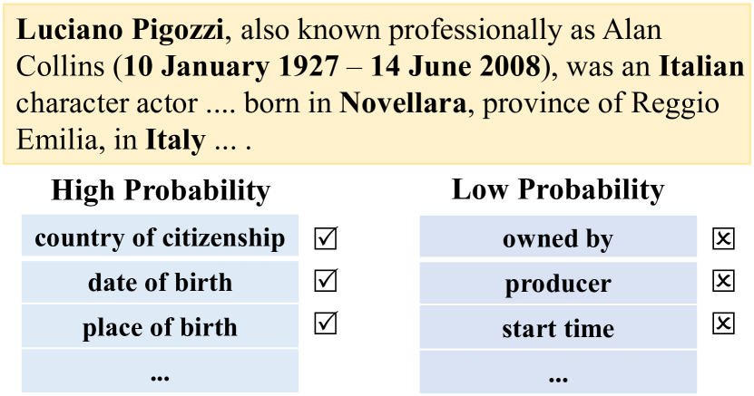
Figure 1: The given document is a biography. Relations “date of birth” and “place of birth” are more likely to occur than other relations such as “‘producer”.

For example, on DocRED dataset Yao et al. (2019), about 60 of the 96 non-NA relations are long-tailed, with less than 200 training triplets. F1 value of these data-scarce relations are even less than 1/3 of data-rich relations. Besides, for entity pairs that express relations, at least 7% have multiple relation labels. With the increase of labels, the F1 value decreases dramatically, by more than 50%. These analyses indicate that the two above challenges cannot be ignored, see Section 2.1 for details. However, existing studies rely heavily on Transformer Zhou et al. (2021); Xie et al. (2022) or rule-based document graph Nan et al. (2020); Zeng et al. (2020); Xu et al. (2021b); Peng et al. (2022b) to obtain contextual representations, ignore the interdependencies among relations and therefore hardly deals with the above challenges.

In this paper, we introduce relation correlations into DocRE task. We argue relations in the real world barely appear independently, they usually interdepend on each other and appear together. For example, the given document in Figure 1 is a personal biography about Luciano Pigozzi, relations “date of birth” and “place of birth” are more likely to be expressed by the document than “producer”. Further, relation “date of birth” is more likely to co-occur with “place of birth” than “producer”. We refer to this co-occurrence between relations as Relation Correlations, which are widely observed, as shown in Figure 3.

Relation correlations can address the above challenges. On the one hand, for long-tailed relations, their correlated relations may be data-rich. By the correlations, data-rich relations can transfer knowledge to data-scarce ones, thus assisting in the training of long-tail relations. On the other hand, for multi-label entity pairs, the same context expresses multiple relations, which means these co-expressed relations are semantically close. The correlations can reflect the semantic distance among relations, which can guide the classifier to identify semantically close relations for multi-label pairs and facilitate the delineation of decision boundaries. See Section 2.1 for detailed analysis.

We first capture the correlations using relation embeddings, and then use the correlation-aware embeddings to guide the classifier to extract relational facts. To improve the perception of relation correlations, we propose two auxiliary co-occurrence prediction sub-tasks from two perspectives, since co-occurrence could reflect correlations explicitly. From the coarse-grained view, relations as labels, Coarse-grained Relation Co-occurrence Prediction (CRCP) task judges whether one relation co-occurs with a set of other relations, based on the relations alone. From the fine-grained view, since relations depend on entity pairs to appear within a document, Fined-grained Relation Co-occurrence Prediction (FRCP) task determines whether one relation co-occurs with a set of other relations, based on both relations and entity pairs.

The learned relation embeddings which could perceive relation correlations thanks to the two auxiliary sub-tasks, accompanied by jointly-trained document contextual representations, are used to extract relational facts.

Substantial experiments on two popular datasets shows that the proposed method not only outperforms the existing baselines but also relieve the two challenges. Our model improves F1 by up to 6.49% on long-tail relations, and up to 12.39% on multi-label entity pairs, demonstrating the effectiveness of introducing relation correlations. We argue that this is the first work to introduce relation correlations into document-level relation extraction task, to the best of our knowledge.

2 Methodology: Introduce Relation Correlations in DocRE

2.1 Motivations

To better illustrate the motivation, we first conduct some data exploration using statistical and experimental analysis.

Statistical Analysis

We conduct statistical analysis on DocRED dataset Yao et al. (2019). The long-tailed distribution is particularly noticeable. More than half of the training triplets express only 6 of the 96 non-NA relation types, and about 60 relation types has less than 200 training instances. In addition, for entity pairs that express relation(s), at least 7% of them have multiple relation labels, which is extremely difficult to identify accurately.

Experimental Analysis

We conduct experiments on long-tailed relations and multi-label entity pairs of DocRED, respectively, using our base model (BERT${}_{\texttt{BASE}}$). See Section 3.1 and  4.1 for details of model and experimental settings.

For long-tailed relations, we calculate the macro-averaged F1 values for all relations (All), data-rich relations (>500) and long-tailed relations (<200 and <100). As shown in the left subfigure of Figure 2, with the reduction of training instances, the performance decreases dramatically. The F1 of “<100” is even less than 1/3 of “>500” (19.84 vs. 65.19). The poor performance of long-tailed relations severely limits the overall performance.

For multi-label entity pairs, we calculate the F1 values when the number of labels is 2, 3, 4, respectively, and report the overall macro-averaged F1. From the right subfigure of Figure 2, we find that the higher the number of labels, the worse the performance. When there are more than 3 labels, the F1 value is substantially lower than the overall value (34.26 vs.51.21).

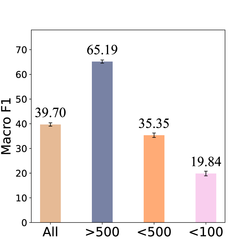
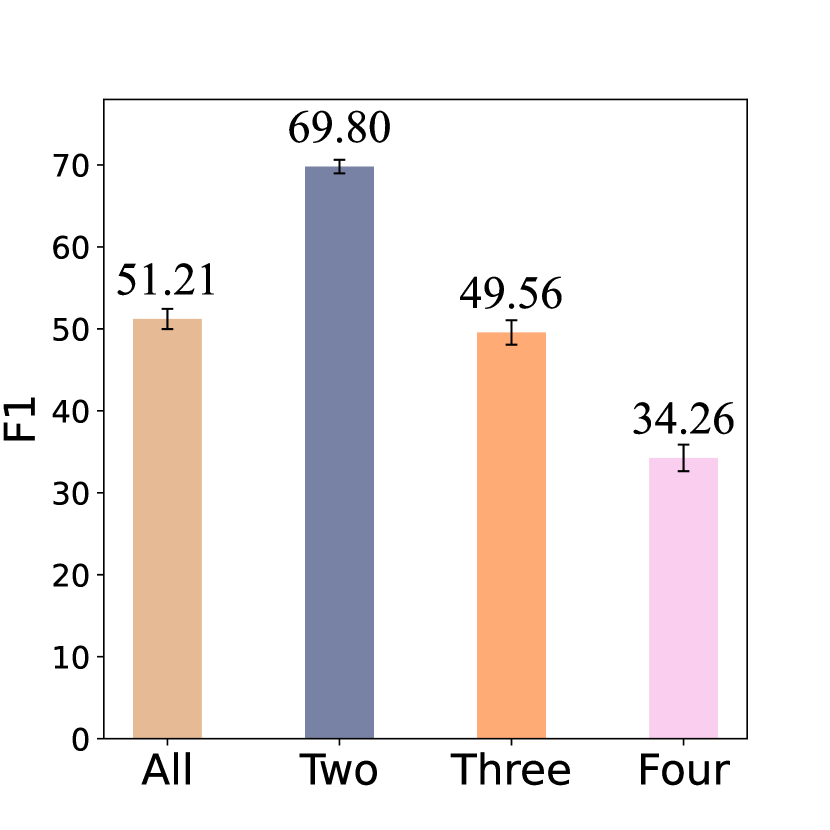
Figure 2: Left figure shows the results of BERT${}_{\texttt{BASE}}$ on long-tailed relations; right figure is the results on multi-label entity pairs. We run 5 times with different seeds, and show the mean and standard deviation bar.

Motivations

Based on the above analyses, we obtain two observations: long-tailed relations are under-trained (i.e., Challenge 1), and the classification of multi-label entity pairs is more challenging than single-label pairs (i.e., Challenge 2).

Existing work hardly deals with the above challenges. Therefore, we introduce relation correlations into DocRE task to alleviate or address them. We observe and analyze the simplest co-occurrence correlation between relations. For example, in Figure 1, relation “place of birth” is more likely to co-occur with “place of date” than “producer”. Further, we count the frequency of co-occurrence between every two relations on DocRED Yao et al. (2019), and use the positive point-wise mutual information values to measure the correlation of relations. As seen in Figure 3, co-occurrence correlation between relations are widely observed.

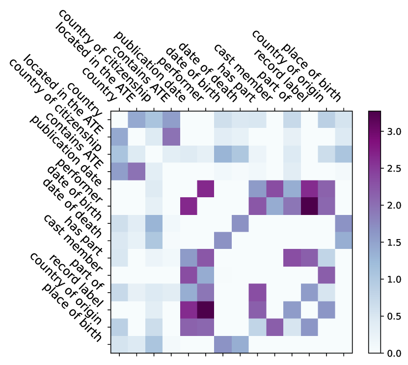
Figure 3: Relation correlations on DocRED. For better visual effect, we only show part of relations. See Appendix B for the complete figure.

Relation correlations can alleviate the above challenges: 1) For long-tailed relations, they may be highly correlated with some data-rich relations. During training, we can transfer knowledge between long-tailed relations and their correlated relations, using data-rich head relations in the long-tail distribution to assist in the training of data-scarce tailed relations, thus alleviating the undertraining caused by insufficient training triplets. 2) For multi-label entity pairs, the same context expresses multiple relations, which means these co-expressed relations have partial semantic overlap. The correlations can reflect the semantic distance among relations. If two relations co-occur frequently, then they are semantically closer than other relations. Such distance information can guide the classifier to identify semantically close relations for multi-label entity pairs, narrowing the search space and facilitating the delineation of decision boundaries.

2.2 DocRE with Relation Correlations

Task Formulation

Suppose a document $d$ consists of $n$ tokens $\{w_{i}\}_{i=1}^{n}$, involving $p$ entities $\{e_{i}\}_{i=1}^{p}$. Each entity $e_{i}$ has $Q_{i}$ mentions $\{m_{j}\}_{j=1}^{Q_{i}}$. Document-level relation extraction task aims to predict one or more relation labels from $\mathcal{R}\cup\{\texttt{NA}\}$ for each entity pair $(e_{s},e_{o})_{s,o=1...p;s\neq o}$, where $\mathcal{R}$ is the set of pre-defined relations, and NA denotes that no relation exists between two entities.

Overview

The overall framework of our model is shown in Figure 4. We first jointly learn document contextual representations and relation embeddings through shared encoder (e.g., BERT), called joint embedding learning (JE). Then, based on relation embeddings, we propose two auxiliary co-occurrence prediction tasks to capture relation correlations from both coarse- and fine-grained perspectives, including Coarse-grained Relation Co-occurrence Prediction (CRCP) and Fine-grained Relation Co-occurrence Prediction (FRCP). Finally, the learned correlation-aware relation embeddings are used to enhance the feature representations of entity pairs, thus guiding relation classification.

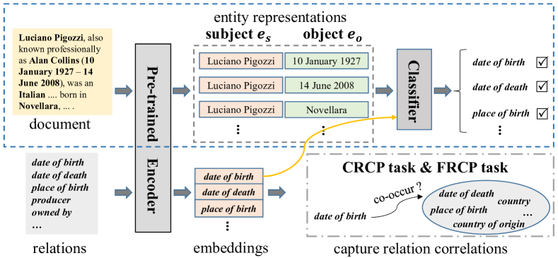
Figure 4: The overall framework of our method. The part circled by blue dashed line is the base model. The orange line indicates that relation embeddings learned by CRCP and FRCP tasks are used to guide relation classification.

Joint Embedding Learning (JE)

To obtain relation embeddings through shared encoder, we combine the document with the sequence of all relations as the inputs to PLMs (e.g., BERT), i.e., “$\texttt{[CLS]}w_{1},w_{2},...,w_{n}\texttt{[SEP]}r_{1},r_{2},...r_{|\mathcal{R}|}\texttt{[SEP]}$ ”, where $r_{i}\in\mathcal{R},i=1,2,...,|\mathcal{R}|$. This method has two strengths: 1) Features and labels can be mapped into the same hidden space, eliminating the semantic gap between relation embeddings and document representations, and 2) Dependencies between document and labels can be automatically captured by stacked self-attention layers.

Since we only share the encoder of base model to obtain the initial relation embeddings, therefore our approach to capturing relation correlations is model-agnostic and can be built on top of existing models. Next, we introduce our proposed sub-tasks in detail. Other implementation details are described in Section 3.

2.2.1 Coarse-grained Relation Co-occurrence Prediction (CRCP)

From the coarse-grained perspective, based on relation labels alone, we judge whether a relation co-occurs with a set of other relations.

For example, suppose the biography in Figure 1 involves five relations, including date of birth, place of birth, date of death, country and country of origin, CRCP task determines whether any one of them should co-occur with the other four relations. It assumes that when the other four relations appear, the remaining one should also be expressed with high probability.

Specifically, one document $d$ has the expressed relation set $R^{+}$ and a unexpressed relation set $R^{-}$. For each $r$ in $R^{+}$, the pair $(r,R^{+}-\{r\})$ serves as a positive example, marked as IsCo-Occur. The task predicts whether target relation $r$ appears based on condition $R^{+}-\{r\}$. By replacing target relation $r$ with one relation $r^{-}$ in $R^{-}$, negative examples $\{(r^{-},R^{+}-\{r\})\}$ can be constructed, marked as NotCo-Occur. The average of the embeddings of $R^{+}-\{r\}$ is concatenated with the embedding of target relation ($r$ or $r^{-}$) as input feature of a binary classifier, obtaining co-occurrence probabilities.

$$p_{ij} =P(r_{j}|d,R^{+}-\{r_{i}\})$$

$$=\sigma(\texttt{{Linear}}([r_{j};\texttt{{Avg}}(R^{+}-\{r_{i}\})]))$$ (1)

We use the binary cross-entropy to calculate the loss value $\mathcal{L}_{coarse}$ for CRCP task, i.e.,

$$\mathcal{L}_{coarse}=-\sum_{i,j}[ q_{ij}\log{p_{ij}}+$$

$$(1-q_{ij})\log{(1-p_{ij})}]$$ (2)

where $q_{ij}$ is the ground-truth (1 means IsCo-Occur and 0 denotes NotCo-Occur).

2.2.2 Fine-grained Relation Co-occurrence Prediction (FRCP)

From the fine-grained perspective, we determine whether a relation co-occurs with a set of other relations based on both relations and entity pairs, since relations depend on entity pairs to appear.

To make relation embeddings better perceive the relation correlations, we propose a surrogate embedding for each entity pair called Relation-Aggregated Embeddings (RAE), which is aggregated using relation embeddings.

Relation-aggregated embedding (RAE)

For each entity pair $(e_{s},e_{o})$, we first calculate matching scores between the pair and all relations using the token-to-relation attention matrix from the last transformer layer of shared encoder, and then use the scores to aggregate relation embeddings. For each entity $e_{i}$, the attention of all its mentions is averaged to be its attention $A_{r,e_{i}}\in\mathbb{R}^{N_{h}\times|r|}$, $N_{h}$ is the number of attention heads.

$$r_{(s,o)}=H_{r}^{\texttt{T}}\cdot\texttt{{Norm}}(\sum_{k=1}^{N_{h}}A_{r,s}^{k}\circ A_{r,o}^{k})$$ (3)

where “$\circ$” denotes hadamard product and $H_{r}$ is the matrix consisting of all relation embeddings. Since attention values are always positive, we use sum normalization, i.e, $\texttt{{Norm}}(\vec{x})=\vec{x}/\textrm{sum}(\vec{x})$.

Positive/negative examples

The resulting $r_{(s,o)}$ can be regarded as the relation representation of entity pair $(e_{s},e_{o})$. Based on whether the entity pair expresses a relation, we divide all relation representations $\{r_{(s,o)}\}_{(s,o)\in d}$ into two groups, non-NA relation set ${R_{\texttt{non-na}}}$ and NA relation set ${R_{\texttt{na}}}$. For each $r_{(s,o)}$ in $R_{\texttt{non-na}}$, the pair $(r_{(s,o)},R_{\texttt{non-na}}-\{r_{(s,o)}\})$ serves as a positive example, marked as IsCo-Occur. The task uses the relations $R_{\texttt{non-na}}-\{r_{(s,o)}\}$ of conditional entity pairs to predict whether the relation $r_{(s,o)}$ of target entity pair co-occurs. By replacing the target relation $r_{(s,o)}$ with one item $r_{\texttt{na}}$ in ${R_{\texttt{na}}}$, negative examples $\{(r_{\texttt{na}},R_{\texttt{non-na}}-\{r_{(s,o)}\})\}$ can be constructed, marked as NotCo-Occur.

A similar thought could be seen in CBOW Mikolov et al. (2013): using context vectors to predict the target. The same implementations as in Eqs. 1 and  2 are used to obtain the co-occurrence probabilities and the loss value $\mathcal{L}_{fine}$.

3 Specific Implementations

3.1 Base Model

We build our base model (BERT${}_{\texttt{BASE}}$) on the existing baselines Wang et al. (2019); Zhou et al. (2021). The document $d=\{w_{i}\}_{i=1}^{n}$ are fed into a pre-trained foundation model (e.g., BERT) to obtain the contextual representations $H=[h_{1},h_{2},...,h_{n}]\in\mathbb{R}^{n\times d_{h}}$, where $d_{h}$ is the embedding dimension.

$$H,A =\texttt{PLMs}([w_{1},w_{2},...,w_{n}])$$ (4)

All entity mentions are wrapped with a special token “*” Zhang et al. (2017); Soares et al. (2019), and the embedding of “*” in front of each mention is regarded as its representation $h_{m_{j}^{i}}$. Next, the log-sum-exp pooling Jia et al. (2019) is employed to get entity embedding $h_{e_{i}}$,

$$h_{e_{i}} =\log{\sum_{j=1}^{N_{e_{i}}}\exp{(h_{m_{j}^{i}})}}$$ (5)

where $N_{e_{i}}$ is the number of mentions for entity $e_{i}$.

As Zhou et al. (2021), the token-to-token attention matrix $A$ of the last transformer layer is used to aggregate context information $c_{(s,o)}\in\mathbb{R}^{d_{h}}$ for each entity pair $(e_{s},e_{o})$. For each entity $e_{i}$, the attention of all its mentions is averaged to be its attention $A_{e_{i}}\in\mathbb{R}^{N_{h}\times n}$.

$$c_{(s,o)}=H^{\texttt{T}}\cdot\textrm{norm}(\sum_{k=1}^{N_{h}}A_{s}^{k}\circ A_{o}^{k})$$ (6)

Finally, entity embeddings $h_{e_{s}}$ and $h_{e_{o}}$ are fused with contextual representation $c_{(s,o)}$, respectively. The resulting representation is fed to the grouped bilinear classifier Tang et al. (2020).

$$f_{s}=\tanh{(W_{s}h_{e_{s}}+W_{1}c_{(s,o)})}$$ (7)

$$f_{o}=\tanh{(W_{o}h_{e_{o}}+W_{2}c_{(s,o)})}$$ (8)

$$P(r|e_{s},e_{o})=\sigma(\sum_{i=1}^{k}{f_{s}^{i}}^{\texttt{T}}W_{r}^{i}f_{o}^{i}+b_{r})$$ (9)

where $[f^{1}_{s};f^{2}_{s};...;f^{k}_{s}]=f_{s}$, $[f^{1}_{o};f^{2}_{o};...;f^{k}_{o}]=f_{o}$, $k$ is the number of groups and $\sigma$ is the sigmoid activation function.

3.2 Base Model with Relation Correlations

To leverage the correlation-aware relation embeddings to guide the classification, we use the relation-aggregated embedding $r_{(s,o)}$ from Eq. 3 as a complementary feature of entity pair $(e_{s},e_{o})$, by modifying Eq. 7 and Eq. 8 as follows:

$$f_{s}=\tanh{(W_{s}h_{e_{s}}+W_{3}[c_{(s,o)};r_{(s,o)}])}$$ (10)

$$f_{o}=\tanh{(W_{o}h_{e_{o}}+W_{4}[c_{(s,o)};r_{(s,o)}])}$$ (11)

where $\{W_{3},W_{4}\}\in\mathbb{R}^{2d_{h}\times d_{h}}$.

Training objective

The main objective for DocRE is defined to minimize a binary cross-entropy loss $\mathcal{L}_{re}$ as Eq. 2. The overall loss can be calculated by:

$$\mathcal{L}_{col}=\alpha\cdot\mathcal{L}_{coarse}+(1-\alpha)\cdot\mathcal{L}_{fine}$$ (12)

$$\mathcal{L}=(1+\beta^{2})\cdot\frac{\mathcal{L}_{re}\cdot\mathcal{L}_{col}}{(\beta^{2}\cdot\mathcal{L}_{col})+\mathcal{L}_{re}}$$ (13)

where $\alpha$ and $\beta$ are trade-off coefficients.

4 Experiments and Analysis

4.1 Experimental Settings

Datasets

To evaluate our proposed model, we conduct experiments on two popular DocRE datasets, i.e., DocREDYao et al. (2019) and DWIEZaporojets et al. (2021). For DWIE, we employ the same pre-processing method as Ru et al. (2021). The statistics are shown in Table 1. Note that we do not choose two other commonly used datasets, i.e., CDRLi et al. (2016) and GDAWu et al. (2019), because they have only one non-NA relationship and are too polarized to model relation correlations.

Dataset	#Train	#Dev	#Test	#Relations
DocRED	3053	998	1000	96
DWIE	602	98	99	65

Table 1: Statistics of DocRED and DWIE datasets.

Implementation Details

We use the popular HuggingFace’s Transformers library (Wolf et al., 2019) to implement our model. For PLMs, we choose the pre-trained BERT-base-cased (Devlin et al., 2019). During training, our model is optimized with AdamW Loshchilov and Hutter (2019) using learning rate $\gamma$. And the warmup technique is also applied. All hyper-parameters are determined on the development set, some of which are listed in Table 2. while during inference, a global threshold determined on the validation set is used to decide whether the relation $r$ exists between $e_{s}$ and $e_{o}$. We search it from the list $[0.1,0.2,...,0.9]$ and pick the one with the highest F1 on the development set. All models are trained with 1 Tesla V100 GPU.

Dataset	DocRED	DWIE
Batch Size	4	4
#Epoch	50	30
lr for PLMs	5e-5	5e-5
lr for others	1e-4	1e-4
ratio for warmup	6%	6%
$\alpha$,$\beta$	0.7,0.5	0.5,0.5

Table 2: Hyper-parameters in training.

Dataset	DocRED				DWIE
	Dev		Test		Dev		Test
Models	Ign. F1	F1	Ign. F1	F1	Ign. F1	F1	Ign. F1	F1
CNN	37.99	43.45	36.44	42.33	37.65	47.73	34.65	46.14
LSTM	44.41	50.66	43.60	50.12	40.86	51.77	40.81	52.60
BiLSTM	45.12	50.95	44.73	51.06	40.46	51.92	42.03	54.47
Context-Aware	44.84	51.10	43.93	50.64	42.06	53.05	45.37	56.58
CorefBERT${}_{\texttt{BASE}}$	55.32	57.51	54.54	56.96	57.18	61.42	61.71	66.59
GAIN${}_{\texttt{BASE}}$	59.14	61.22	59.00	61.24	58.63	62.55	62.37	67.57
SSAN${}_{\texttt{BASE}}$	57.04	59.19	56.06	58.41	58.62	64.49	62.58	69.39
ATLOP${}_{\texttt{BASE}}$	59.22	61.09	59.31	61.30	59.03	64.82	62.09	69.94
ERA${}_{\texttt{BASE}}$	59.30	61.30	58.71	60.97	-	-	-	-
ERACL${}_{\texttt{BASE}}$	59.72	61.80	59.08	61.36	-	-	-	-
RSMAN${}_{\texttt{SSAN-BASE}}$	57.22	59.25	57.02	59.29	60.02	65.88	63.42	70.95
BERT${}_{\texttt{BASE}}$	58.09$\pm$0.11	60.10$\pm$0.12	58.03	60.20	58.40$\pm$0.26	63.38$\pm$0.33	62.92$\pm$0.64	69.12$\pm$0.56
BERT-Correl${}_{\texttt{BASE}}$	59.39${}^{\dagger}\pm$0.13	61.34${}^{\dagger}\pm$0.11	59.12	61.32	61.10${}^{\dagger}\pm$0.54	65.73${}^{\dagger}\pm$0.69	65.64${}^{\dagger}\pm$0.52	71.56${}^{\dagger}\pm$0.28
	$\uparrow$1.30	$\uparrow$1.24	$\uparrow$1.09	$\uparrow$1.12	$\uparrow$1.70	$\uparrow$2.35	$\uparrow$2.72	$\uparrow$2.44
- CRCP	59.03$\pm$0.09	60.97$\pm$0.05	58.89	61.03	59.40$\pm$0.43	64.38$\pm$0.74	64.87$\pm$1.29	70.90$\pm$0.90
- FRCP	59.11$\pm$0.12	61.10$\pm$0.09	59.05	61.12	59.52$\pm$0.28	64.00$\pm$0.26	64.33$\pm$0.54	69.99$\pm$0.52
- CRCP and FRCP	58.33$\pm$0.23	60.24$\pm$0.20	58.38	60.45	58.97$\pm$0.13	63.92$\pm$0.47	63.72$\pm$0.64	69.72$\pm$0.61
- JE (BERT${}_{\texttt{BASE}}$)	58.09$\pm$0.11	60.10$\pm$0.12	58.03	60.20	58.40$\pm$0.26	63.38$\pm$0.33	62.92$\pm$0.64	69.12$\pm$0.56

Table 3: Main results (%) on DocRED and DWIE datasets. We run 5 times with different random seeds, and report the mean and standard deviation (excluding the results of DocRED’s test set, as it must be obtained through CodaLab site). For DocRED, the results are from their original paper, while for DWIE, we use the results reported in Yu et al. (2022). The subscript “BASE” indicates using BERT-base as the backbone encoder. ^† indicates that the improvement is significant according to a two-sided T-Test ($p<0.05$).

Metrics

For overall performance, we use micro F1 and Ign. F1 in evaluation. The Ign. F1 denotes the F1 value after excluding entity pairs that appear in both train and development/test set. For long-tailed relations, we report the Macro@K which means the macro-averaged F1 for relation types with frequency in training set less than $K$. Compared to micro-F1, macro-F1 treat all relation types equally and can more accurately reflect the performance on long-tailed relations. While for multi-label entity pairs, we report the micro-F1 value when there are two/three/four labels.

Baselines

We compare our model with some typical or recent baselines, including CNN Zeng et al. (2014), LSTM/BiLSTM Cai et al. (2016), Context-Aware Sorokin and Gurevych (2017), CorefBERT Ye et al. (2020), GAIN Zeng et al. (2020), SSAN Xu et al. (2021a), ATLOP Zhou et al. (2021), ERA/ERACL Du et al. (2022) and RSMAN Yu et al. (2022).

4.2 Model Comparison Results

Table 3 depicts the overall performance of our proposed model on two popular DocRE datasets, in comparison with baselines. We can find that our base model (BERT${}_{\texttt{BASE}}$) outperforms some earlier BERT-based baselines, CorefBERT${}_{\texttt{BASE}}$ Ye et al. (2020) and SSAN Xu et al. (2021a), on all result columns of DocRED and DWIE datasets. In other words, our base model yields strong performance compared to the earlier BERT-based models. Further, our model BERT-Correl${}_{\texttt{BASE}}$ improves the performance of BERT${}_{\texttt{BASE}}$ by 1.30%, 1.24%, 1.09%, 1.12% for each column on DocRED dataset and 1.70%, 2.35%, 2.72%, 2.44% for each column on DWIE dataset. The improvement is consistent, which confirms the generalization of our approach. All results pass the two-sided T-Test ($p<0.05$), indicating that the improvement is significant.

Dataset	DocRED				DWIE
	Macro	Macro@500	Macro@200	Macro@100	Macro	Macro@100	Macro@50
BERT${}_{\texttt{BASE}}$	39.70$\pm$0.47	35.35$\pm$0.59	27.66$\pm$0.71	19.84$\pm$0.64	28.17$\pm$0.40	6.53$\pm$0.55	2.47$\pm$0.50
BERT-Correl${}_{\texttt{BASE}}$	40.81${}^{\dagger}\pm$0.35	36.55${}^{\dagger}\pm$0.40	28.76${}^{\dagger}\pm$0.63	21.38${}^{\dagger}\pm$0.96	32.80${}^{\dagger}\pm$1.25	13.02${}^{\dagger}\pm$1.46	8.59${}^{\dagger}\pm$1.73
	$\uparrow$1.11	$\uparrow$1.20	$\uparrow$1.10	$\uparrow$1.54	$\uparrow$4.63	$\uparrow$6.49	$\uparrow$6.12
- CRCP	40.48$\pm$0.32	36.18$\pm$0.36	28.32$\pm$0.39	20.56$\pm$0.54	30.52$\pm$0.63	10.24$\pm$0.94	5.98$\pm$1.47
- FRCP	40.52$\pm$0.32	36.22$\pm$0.32	28.53$\pm$0.51	20.52$\pm$0.67	30.46$\pm$0.99	10.47$\pm$1.46	6.19$\pm$1.47
- CRCP and FRCP	39.77$\pm$0.57	35.47$\pm$0.62	27.63$\pm$0.64	19.93$\pm$0.52	27.81$\pm$0.41	5.62$\pm$0.43	1.88$\pm$0.64
- JE (BERT${}_{\texttt{BASE}}$)	39.70$\pm$0.47	35.35$\pm$0.59	27.66$\pm$0.71	19.84$\pm$0.64	28.17$\pm$0.40	6.53$\pm$0.55	2.47$\pm$0.50

Table 4: Evaluation on long-tailed relations. We run 5 times with different random seeds on the development set, and report the mean and standard deviation. Labels of DocRED’s test set are not accessible, so the values on test set cannot be displayed. ^† indicates that the improvement is significant according to a two-sided T-Test ($p<0.05$).

Dataset	DocRED				DWIE
	Two	Three	Four	Macro F1	Two	Three	Macro F1
BERT${}_{\texttt{BASE}}$	69.80$\pm$0.69	49.56$\pm$1.49	34.26$\pm$1.62	51.21$\pm$1.17	70.13$\pm$0.59	77.11$\pm$1.03	73.62$\pm$0.38
BERT-Correl${}_{\texttt{BASE}}$	70.97${}^{\dagger}\pm$0.73	55.16${}^{\dagger}\pm$0.58	46.65${}^{\dagger}\pm$1.95	57.59${}^{\dagger}\pm$0.63	73.98${}^{\dagger}\pm$1.63	79.29${}^{\dagger}\pm$1.41	76.63${}^{\dagger}\pm$0.86
	$\uparrow$1.17	$\uparrow$5.60	$\uparrow$12.39	$\uparrow$6.38	$\uparrow$3.85	$\uparrow$2.18	$\uparrow$3.01
- CRCP	70.53$\pm$1.31	56.40$\pm$1.22	39.99$\pm$0.82	55.64$\pm$0.90	71.91$\pm$1.20	78.13$\pm$1.34	75.02$\pm$1.12
- FRCP	70.64$\pm$0.83	55.42$\pm$1.81	41.88$\pm$1.33	55.98$\pm$0.57	71.17$\pm$0.57	78.30$\pm$1.33	74.74$\pm$0.71
- CRCP and FRCP	69.92$\pm$0.80	51.49$\pm$1.92	40.00$\pm$0.01	53.80$\pm$0.72	70.01$\pm$0.74	76.22$\pm$0.82	73.11$\pm$0.61
- JE (BERT${}_{\texttt{BASE}}$)	69.80$\pm$0.83	49.56$\pm$1.49	34.26$\pm$1.62	51.21$\pm$1.23	70.13$\pm$0.59	77.11$\pm$1.03	73.62$\pm$0.38

Table 5: Results on multi-label entity pairs. We run 5 times with different random seeds, and report the mean and standard deviation. ^† indicates that the improvement is significant according to a two-sided T-Test ($p<0.05$).

4.3 Ablation Study

To show the efficacy of each component, we conduct ablation studies on both DocRED and DWIE, by turning off one component at a time. The results are shown at the bottom of Table 3. We can find that without CRCP and FRCP, the model performance has no or little improvement over the base model BERT-Correl${}_{\texttt{BASE}}$. (Please refer to the bottom two rows of Table 3, here -JE indicates the model for further disabling the JE module when CRCP and FRCP are not enabled, which is the same as BERT-Correl${}_{\texttt{BASE}}$.) When either CRCP or FRCP is enabled, the model achieves a significant performance improvement over BERT-Correl${}_{\texttt{BASE}}$. This observation also demonstrates that our proposed sub-tasks, CRCP and FRCP, are both very effective, and that introducing relation correlations into DocRE scenario is highly powerful. Moreover, when we enable both CRCP and FRCP, the performance is improved by at least 1.09% on DocRED and at least 1.70% on DWIE.

4.4 Analysis and Visualization

Results on Long-tailed Relations

To explore the impact of relation correlations on long-tailed relations, we conduct experiments on the tailed relation types which has fewer than $K$ training instances/ triplets. Then we report the macro-averaged F1 (Macro@K) for relation types with less than $K$ training instances in Table 4. $K$ selects values of 500, 200 and 100 for DocRED, while for DWIE, $K$ selects values of 100 and 50. “Macro” denotes the macro-averaged F1 for all relation types. We can find that our model BERT-Correl${}_{\texttt{BASE}}$ achieves consistent performance gains on long-tail relations for both DocRED and DWIE datasets, mitigating the Long-tail problem. The fewer training instances, the greater the improvement. In particular, for DWIE dataset, the performance improvement of macro-averaged F1 on tailed relations is over 6%, which indicates relation correlations has great potential for addressing long-tail relation classification. The two-sided T-Test are also employed to verify the significance of the improvement.

Results on Multi-Label Entity Pairs

We select all entity pairs expressing multiple relation types from the development set, and evaluate our model on them. Since the labels of DocRED’s test set are not available, the results on test set cannot be reported, we just report the results on the development set. Detailed results are shown in Table 5. Here multiple labels of an entity pair are individually judged to be correct or not, and counted separately. If an entity pair has 2 labels, then there are two relational triplets to evaluate. We find that relation correlations delivers consistent improvement on multi-label entity pairs of two datasets. The higher the number of labels, the more significant the improvement. In particular, for entity pairs with 4 labels on DocRED, our BERT-Correl${}_{\texttt{BASE}}$ improves by 12.39%.

Visualization of Relation Correlations

We use the relation embeddings learned by our model on DocRED for visualization. We employ dot-product to calculate the relation similarity matrix, and visualize it in Figure 5. For each row, we only display top-8 correlated relations for better visual effect. We find Figure 5 similar to Figure 3, implying that we do capture large amounts of correlation knowledge based on CRCP task and FRCP task.

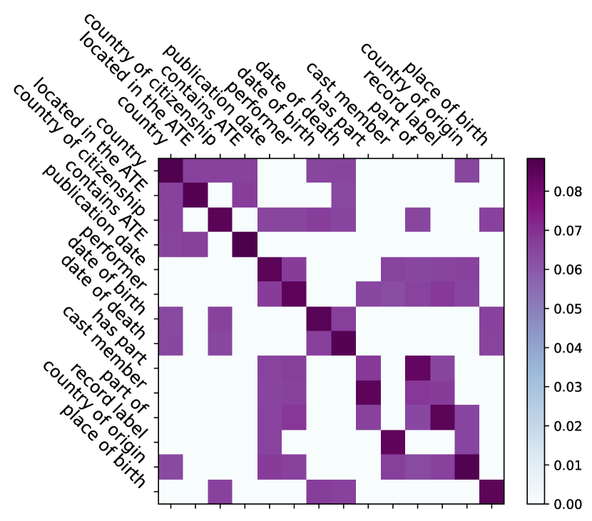
Figure 5: Relation correlations learned by our model on DocRED. For better visual effect, we only show part of relations as Figure 3.

5 Related Work

Sentence-level Relation Extraction

Sentence-level relation extraction mainly includes CNN-based methods Zeng et al. (2014); dos Santos et al. (2015); Zeng et al. (2015); Peng et al. (2022a), RNN-based methods Zhang et al. (2015); Cai et al. (2016), GNN-based methods Zhang et al. (2018); Zhu et al. (2019) and attention-based methods Lin et al. (2016); Dai et al. (2019); Ye and Ling (2019); Yuan et al. (2019); Han et al. (2022). These methods mainly benefit from local features Peng et al. (2020) such as entity type, entity position, etc. In DocRE, these local features are far from sufficient, the global cross-sentence dependencies and reasoning are necessary.

Document-level Relation Extraction

Existing work on document-level relation extraction can be mainly divided into three categories, including sequence-based models Yao et al. (2019), graph-based models Nan et al. (2020); Zeng et al. (2020); Xu et al. (2021b, c); Li et al. (2022); Peng et al. (2022b) and Transformer-based models Zhou et al. (2021); Yu et al. (2022); Xie et al. (2022). The sequence-based models use CNN Goodfellow et al. (2016) or LSTM Schuster and Paliwal (1997) to encode the entire document directly, just copying the SentRE models and yielding poor performance. The graph-based models construct document graphs based on heuristic rules, encoding with graph neural networks Veličković et al. (2018), achieving high performance. Unlike the graph-based models that rely heavily on handcrafted rules, the Transformer-based models leverage the capability for long-range dependencies of PLMs to directly obtain entity embeddings and contextual representations.

Relation Correlations

None of the above methods consider relation correlations. Similar to label correlations in the multi-label learning field Zhu et al. (2018); Zhang and Zhou (2014), relation correlations are originally proposed by Jin et al. (2020), they define this phenomenon as “Relation of Relations (ROR)” through statistical analysis. Then Peng et al. (2022a) and Han et al. (2022) introduce relation correlations into the hierarchical relation extraction task under the distant supervision paradigm, and achieve state-of-the-art performance. However, both studies perform sentence-level RE where the relation types have a hierarchical taxonomic structure. As clues, the structure can be directly used to model the correlations. In contrast, this paper focuses on DocRE task that the taxonomic structure does not exist, which is more challenging to capture the correlations.

6 Conclusion

In this paper, we analyze DocRE task in depth, and draw two observations: 1) The long-tailed relations are under-trained (i.e., challenge 1), and 2) The classification of multi-label entity pair is more challenging than single-label pairs (i.e., challenge 2). We analyze the co-occurrence correlation of relations, and introduce it into DocRE task.

We deem that relation correlations can alleviate the above challenges: 1) The correlations can transfer knowledge between data-rich relations and data-scarce long-tailed ones, assisting in the training of tailed relations, and 2) The correlations can reflect semantic distance among relations, and guide the classifier to identify semantically close relations for multi-label pairs. Specifically, we first jointly learn the relation embeddings with document representations. Then, two auxiliary co-occurrence prediction sub-tasks (i.e., CRCP and FRCP) are designed to capture the correlations using relation embeddings. Finally, the learned correlation-aware relation embeddings are used to guide the classification. We conduct experiments on two popular datasets. Relation correlations not only bring consistent improvements in overall RE performance, but also show strong potential for long-tail relations and multi-label entity pairs.

Appendix A Supplementary Details of Experiments

Dataset

As stated in Section 4.1, we evaluate our model on DocRED and DWIE datasets. DocRED is the first large-scale crowdsourced dataset for document-level relation extraction, which is constructed from Wikipedia articles. DWIE is a dataset for document-level multi-task information extraction which contains four sub-tasks. To make it suitable for the DocRE task, the same preprocessing method as Ru et al. (2021) is applied.

More statistical information on training set of these two datasets is detailed in Tabel 6. We see that each document on DocRED contains 19.49 entities expressing 12.51 relational facts, on average. Similar observations are made on DWIE. And the number of multi-label entity pairs on two datasets are 2466 and 2880, respectively. These observations also support the multi-entity and multi-label properties of DocRE task.

Statistics	DocRED	DWIE
#Relation Facts	38180	14410
#Multi-label Entity pairs	2466	2880
Avg.#Entities per Doc.	19.49	27.4
Avg.#Mentions per Entity	1.34	1.97
Avg.#Relation Facts per Doc.	12.51	23.94

Table 6: More statistical information of training set on DocRED and DWIE datasets.

Parameters Setting

For the general hyper-parameters such as batch size, learning rate, etc., we set them to be consistent with Zhou et al. (2021). For the coefficients (i.e., $\alpha$ and $\beta$) of training objectives, we search them from the list $[0.1,0.2,...,0.9]$ and pick the one with the highest F1 on the development set.

Appendix B Statistical Correlation Matrices

In this section, we show the complete statistical figures of relation correlations for the DocRED Yao et al. (2019) and DWIE Zaporojets et al. (2021) datasets. We first count the frequency of co-occurrence between every two relations, and then calculate the positive point-wise mutual information values to measure the correlations. Relation ids are sorted in descending order by the number of training triplets. For better visual effect, we only display top-20 correlated relations for each row. Since the correlation values of DWIE vary dramatically, we truncate all values greater than 1.5. In Figure 6, we can find that the co-occurrence correlation of relations is widespread, which is an essential inherent characteristic of the training data itself.

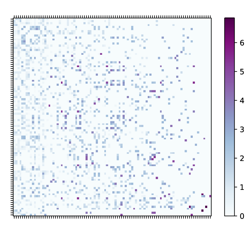
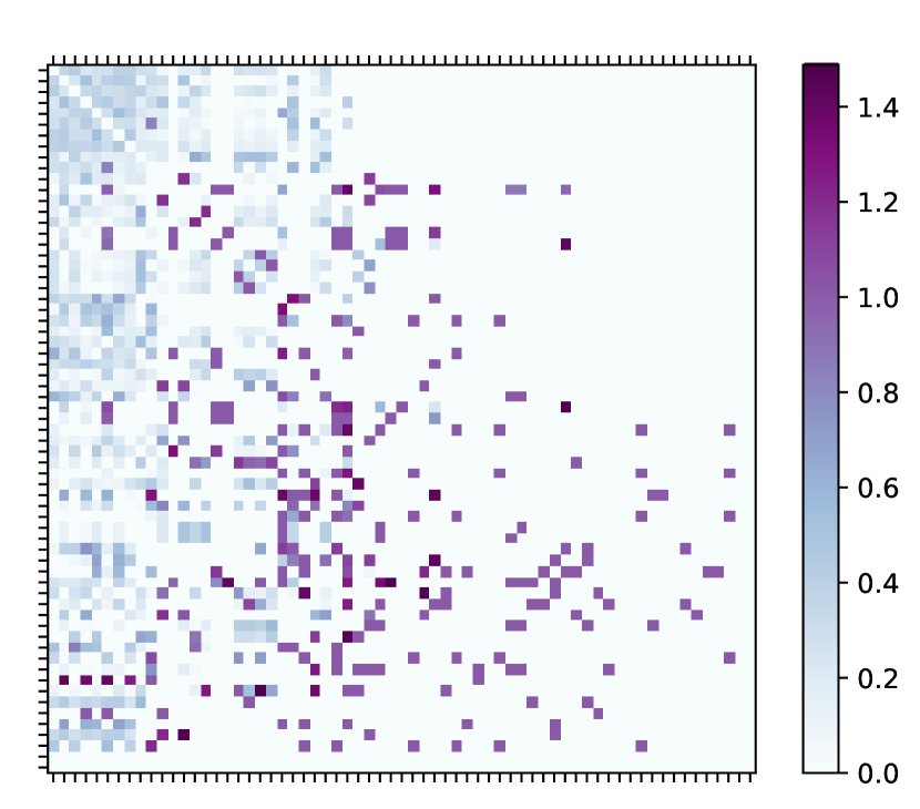
Figure 6: Statistical Relation correlations on DocRED (left) and DWIE (right) datasets. For better visual effect, we only display top-20 correlated relations for each row. For DWIE, we truncate all values greater than 1.5.

Appendix C Long-tail Distribution of Relations

We count the frequency of relations in the training set of DocRED and DWIE datasets, and display the distributions in Figure 7. Relation ids are also sorted by frequency count from high to low. The green dashed lines separate data-rich relations from long-tail ones. Here the relations with less than 200 training instances are considered as long-tail relations, and vice versa for data-rich relations. We can find that most of the relations are long-tailed on both DocRED and DWIE datasets. The lack of training instances makes these relations under-trained, severely limiting the performance of DocRE task.

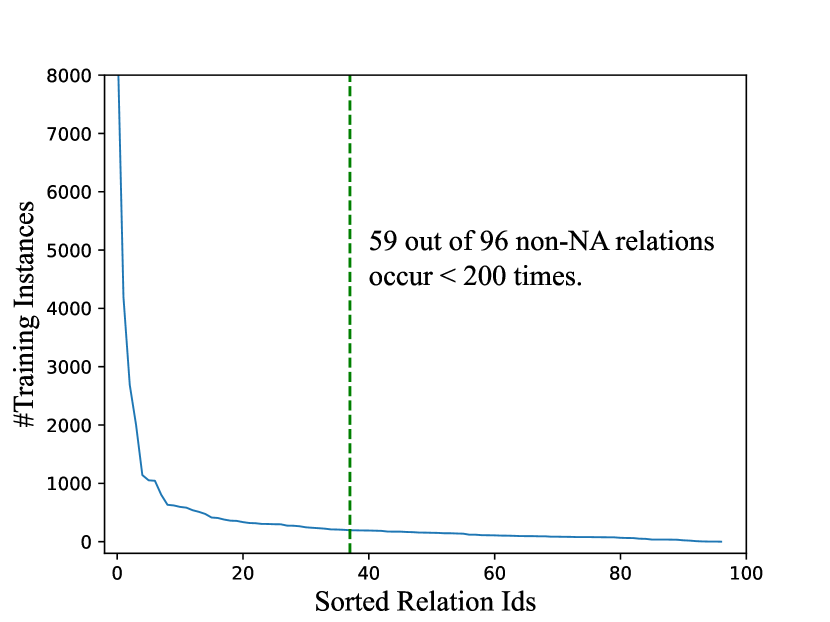
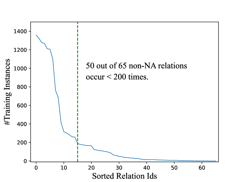
Figure 7: Relation distribution of training set on DocRED (left) and DWIE (right) datasets.

Appendix D The Learned Correlation Matrices

To check the correlations learned by our model, we fetch the relation embeddings learned by our model on DocRED and DWIE datasets, employ dot-product to calculate the relation similarity correlation matrices, and visual the complete matrices in Figure 8. Same as Appendix B, relation ids are also sorted in descending order by the number of training triplets. For better visual effect, we only display top-8 correlated relations for each row. Although there are some noise points, we can find that the correlation matrices we learned are very similar to Figure 6. This observation implies that our model does capture large amounts of correlation knowledge.

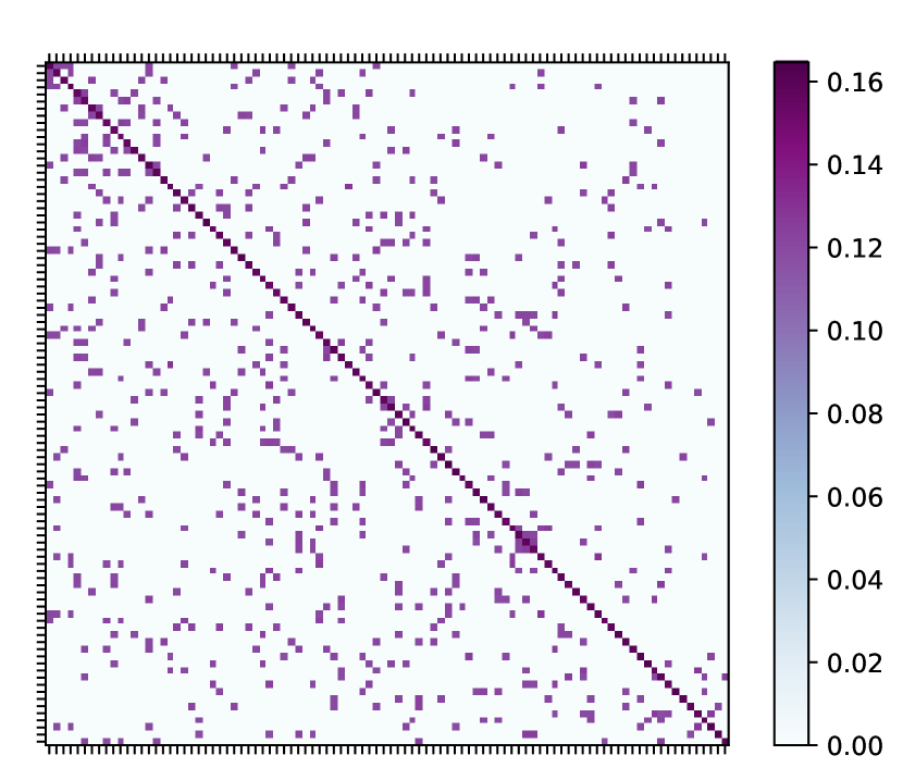
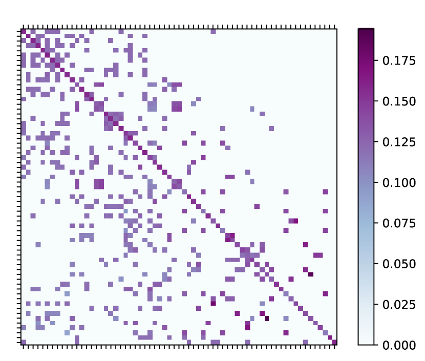
Figure 8: The learned relation correlations on DocRED (left) and DWIE (right) datasets.

References

- Cai et al. (2016) Rui Cai, Xiaodong Zhang, and Houfeng Wang. 2016. Bidirectional recurrent convolutional neural network for relation classification. In Proceedings of the 54th Annual Meeting of the Association for Computational Linguistics, ACL. The Association for Computer Linguistics.
- Dai et al. (2019) Longqi Dai, Bo Xu, and Hui Song. 2019. Feature-level attention based sentence encoding for neural relation extraction. In Natural Language Processing and Chinese Computing - 8th CCF International Conference, NLPCC, volume 11838 of Lecture Notes in Computer Science, pages 184–196. Springer.
- Devlin et al. (2019) Jacob Devlin, Ming-Wei Chang, Kenton Lee, and Kristina Toutanova. 2019. BERT: pre-training of deep bidirectional transformers for language understanding. In Proceedings of the 2019 Conference of the North American Chapter of the Association for Computational Linguistics: Human Language Technologies, NAACL-HLT, pages 4171–4186. Association for Computational Linguistics.
- dos Santos et al. (2015) Cícero Nogueira dos Santos, Bing Xiang, and Bowen Zhou. 2015. Classifying relations by ranking with convolutional neural networks. In Proceedings of the 53rd Annual Meeting of the Association for Computational Linguistics and the 7th International Joint Conference on Natural Language Processing of the Asian Federation of Natural Language Processing, ACL, pages 626–634. The Association for Computer Linguistics.
- Du et al. (2022) Yangkai Du, Tengfei Ma, Lingfei Wu, Yiming Wu, Xuhong Zhang, Bo Long, and Shouling Ji. 2022. Improving long tailed document-level relation extraction via easy relation augmentation and contrastive learning. CoRR, abs/2205.10511.
- Goodfellow et al. (2016) Ian J. Goodfellow, Yoshua Bengio, and Aaron C. Courville. 2016. Deep Learning. Adaptive Computation and Machine Learning. MIT Press.
- Han et al. (2022) Ridong Han, Tao Peng, Jiayu Han, Hai Cui, and Lu Liu. 2022. Distantly supervised relation extraction via recursive hierarchy-interactive attention and entity-order perception. Neural Networks, 152:191–200.
- Jia et al. (2019) Robin Jia, Cliff Wong, and Hoifung Poon. 2019. Document-level n-ary relation extraction with multiscale representation learning. In Proceedings of the 2019 Conference of the North American Chapter of the Association for Computational Linguistics: Human Language Technologies, NAACL-HLT, pages 3693–3704. Association for Computational Linguistics.
- Jin et al. (2020) Zhijing Jin, Yongyi Yang, Xipeng Qiu, and Zheng Zhang. 2020. Relation of the relations: A new paradigm of the relation extraction problem. CoRR, abs/2006.03719.
- Li et al. (2016) Jiao Li, Yueping Sun, Robin J. Johnson, Daniela Sciaky, Chih-Hsuan Wei, Robert Leaman, Allan Peter Davis, Carolyn J. Mattingly, Thomas C. Wiegers, and Zhiyong Lu. 2016. Biocreative V CDR task corpus: a resource for chemical disease relation extraction. Database J. Biol. Databases Curation, 2016.
- Li et al. (2022) Lishuang Li, Ruiyuan Lian, Hongbin Lu, and Jingyao Tang. 2022. Document-level biomedical relation extraction based on multi-dimensional fusion information and multi-granularity logical reasoning. In Proceedings of the 29th International Conference on Computational Linguistics, COLING, pages 2098–2107. International Committee on Computational Linguistics.
- Lin et al. (2016) Yankai Lin, Shiqi Shen, Zhiyuan Liu, Huanbo Luan, and Maosong Sun. 2016. Neural relation extraction with selective attention over instances. In Proceedings of the 54th Annual Meeting of the Association for Computational Linguistics, ACL. The Association for Computer Linguistics.
- Loshchilov and Hutter (2019) Ilya Loshchilov and Frank Hutter. 2019. Decoupled weight decay regularization. In Proceedings of the 7th International Conference on Learning Representations, ICLR. OpenReview.net.
- Mikolov et al. (2013) Tomás Mikolov, Kai Chen, Greg Corrado, and Jeffrey Dean. 2013. Efficient estimation of word representations in vector space. In 1st International Conference on Learning Representations, ICLR, Workshop Track Proceedings.
- Nan et al. (2020) Guoshun Nan, Zhijiang Guo, Ivan Sekulic, and Wei Lu. 2020. Reasoning with latent structure refinement for document-level relation extraction. In Proceedings of the 58th Annual Meeting of the Association for Computational Linguistics, ACL, pages 1546–1557. Association for Computational Linguistics.
- Peng et al. (2020) Hao Peng, Tianyu Gao, Xu Han, Yankai Lin, Peng Li, Zhiyuan Liu, Maosong Sun, and Jie Zhou. 2020. Learning from context or names? an empirical study on neural relation extraction. In Proceedings of the 2020 Conference on Empirical Methods in Natural Language Processing, EMNLP, pages 3661–3672. Association for Computational Linguistics.
- Peng et al. (2022a) Tao Peng, Ridong Han, Hai Cui, Lin Yue, Jiayu Han, and Lu Liu. 2022a. Distantly supervised relation extraction using global hierarchy embeddings and local probability constraints. Knowledge-Based Systems., 235:107637.
- Peng et al. (2022b) Xingyu Peng, Chong Zhang, and Ke Xu. 2022b. Document-level relation extraction via subgraph reasoning. In Proceedings of the Thirty-First International Joint Conference on Artificial Intelligence, IJCAI, pages 4331–4337. ijcai.org.
- Ru et al. (2021) Dongyu Ru, Changzhi Sun, Jiangtao Feng, Lin Qiu, Hao Zhou, Weinan Zhang, Yong Yu, and Lei Li. 2021. Learning logic rules for document-level relation extraction. In Proceedings of the 2021 Conference on Empirical Methods in Natural Language Processing, EMNLP, pages 1239–1250. Association for Computational Linguistics.
- Schuster and Paliwal (1997) Mike Schuster and Kuldip K. Paliwal. 1997. Bidirectional recurrent neural networks. IEEE Trans. Signal Process., 45(11):2673–2681.
- Soares et al. (2019) Livio Baldini Soares, Nicholas FitzGerald, Jeffrey Ling, and Tom Kwiatkowski. 2019. Matching the blanks: Distributional similarity for relation learning. In Proceedings of the 57th Conference of the Association for Computational Linguistics, ACL, pages 2895–2905. Association for Computational Linguistics.
- Sorokin and Gurevych (2017) Daniil Sorokin and Iryna Gurevych. 2017. Context-aware representations for knowledge base relation extraction. In Proceedings of the 2017 Conference on Empirical Methods in Natural Language Processing, EMNLP, pages 1784–1789. Association for Computational Linguistics.
- Tang et al. (2020) Yun Tang, Jing Huang, Guangtao Wang, Xiaodong He, and Bowen Zhou. 2020. Orthogonal relation transforms with graph context modeling for knowledge graph embedding. In Proceedings of the 58th Annual Meeting of the Association for Computational Linguistics, ACL, pages 2713–2722. Association for Computational Linguistics.
- Vashishth et al. (2018) Shikhar Vashishth, Rishabh Joshi, Sai Suman Prayaga, Chiranjib Bhattacharyya, and Partha P. Talukdar. 2018. RESIDE: improving distantly-supervised neural relation extraction using side information. In Proceedings of the 2018 Conference on Empirical Methods in Natural Language Processing, EMNLP, pages 1257–1266. Association for Computational Linguistics.
- Veličković et al. (2018) Petar Veličković, Guillem Cucurull, Arantxa Casanova, Adriana Romero, Pietro Liò, and Yoshua Bengio. 2018. Graph attention networks. In Proceedings of the 6th International Conference on Learning Representations, ICLR. OpenReview.net.
- Wang et al. (2019) Hong Wang, Christfried Focke, Rob Sylvester, Nilesh Mishra, and William Yang Wang. 2019. Fine-tune bert for docred with two-step process. CoRR, abs/1909.11898.
- Wolf et al. (2019) Thomas Wolf, Lysandre Debut, Victor Sanh, Julien Chaumond, Clement Delangue, Anthony Moi, Pierric Cistac, Tim Rault, Rémi Louf, Morgan Funtowicz, and Jamie Brew. 2019. Huggingface’s transformers: State-of-the-art natural language processing. CoRR, abs/1910.03771.
- Wu et al. (2019) Ye Wu, Ruibang Luo, Henry C. M. Leung, Hing-Fung Ting, and Tak Wah Lam. 2019. RENET: A deep learning approach for extracting gene-disease associations from literature. In Research in Computational Molecular Biology - 23rd Annual International Conference, RECOMB, volume 11467 of Lecture Notes in Computer Science, pages 272–284. Springer.
- Xie et al. (2022) Yiqing Xie, Jiaming Shen, Sha Li, Yuning Mao, and Jiawei Han. 2022. Eider: Empowering document-level relation extraction with efficient evidence extraction and inference-stage fusion. In Findings of the Association for Computational Linguistics: ACL, pages 257–268. Association for Computational Linguistics.
- Xu et al. (2021a) Benfeng Xu, Quan Wang, Yajuan Lyu, Yong Zhu, and Zhendong Mao. 2021a. Entity structure within and throughout: Modeling mention dependencies for document-level relation extraction. In Proceedings of the Thirty-Fifth AAAI Conference on Artificial Intelligence, AAAI, pages 14149–14157. AAAI Press.
- Xu et al. (2021b) Wang Xu, Kehai Chen, and Tiejun Zhao. 2021b. Discriminative reasoning for document-level relation extraction. In Findings of the Association for Computational Linguistics: ACL/IJCNLP, pages 1653–1663. Association for Computational Linguistics.
- Xu et al. (2021c) Wang Xu, Kehai Chen, and Tiejun Zhao. 2021c. Document-level relation extraction with reconstruction. In Proceedings of the Thirty-Fifth AAAI Conference on Artificial Intelligence, AAAI, pages 14167–14175. AAAI Press.
- Yao et al. (2019) Yuan Yao, Deming Ye, Peng Li, Xu Han, Yankai Lin, Zhenghao Liu, Zhiyuan Liu, Lixin Huang, Jie Zhou, and Maosong Sun. 2019. Docred: A large-scale document-level relation extraction dataset. In Proceedings of the 57th Conference of the Association for Computational Linguistics, ACL, pages 764–777. Association for Computational Linguistics.
- Ye et al. (2020) Deming Ye, Yankai Lin, Jiaju Du, Zhenghao Liu, Peng Li, Maosong Sun, and Zhiyuan Liu. 2020. Coreferential reasoning learning for language representation. In Proceedings of the 2020 Conference on Empirical Methods in Natural Language Processing, EMNLP, pages 7170–7186. Association for Computational Linguistics.
- Ye and Ling (2019) Zhi-Xiu Ye and Zhen-Hua Ling. 2019. Distant supervision relation extraction with intra-bag and inter-bag attentions. In Proceedings of the 2019 Conference of the North American Chapter of the Association for Computational Linguistics: Human Language Technologies, NAACL-HLT, pages 2810–2819. Association for Computational Linguistics.
- Yu et al. (2022) Jiaxin Yu, Deqing Yang, and Shuyu Tian. 2022. Relation-specific attentions over entity mentions for enhanced document-level relation extraction. In Proceedings of the 2022 Conference of the North American Chapter of the Association for Computational Linguistics: Human Language Technologies, NAACL, pages 1523–1529. Association for Computational Linguistics.
- Yuan et al. (2019) Yujin Yuan, Liyuan Liu, Siliang Tang, Zhongfei Zhang, Yueting Zhuang, Shiliang Pu, Fei Wu, and Xiang Ren. 2019. Cross-relation cross-bag attention for distantly-supervised relation extraction. In Proceedings of The Thirty-Third AAAI Conference on Artificial Intelligence, AAAI, pages 419–426. AAAI Press.
- Zaporojets et al. (2021) Klim Zaporojets, Johannes Deleu, Chris Develder, and Thomas Demeester. 2021. DWIE: an entity-centric dataset for multi-task document-level information extraction. Information Processing & Management., 58(4):102563.
- Zeng et al. (2015) Daojian Zeng, Kang Liu, Yubo Chen, and Jun Zhao. 2015. Distant supervision for relation extraction via piecewise convolutional neural networks. In Proceedings of the 2015 Conference on Empirical Methods in Natural Language Processing, EMNLP, pages 1753–1762. The Association for Computational Linguistics.
- Zeng et al. (2014) Daojian Zeng, Kang Liu, Siwei Lai, Guangyou Zhou, and Jun Zhao. 2014. Relation classification via convolutional deep neural network. In Proceedings of the 25th International Conference on Computational Linguistics, COLING, pages 2335–2344. ACL.
- Zeng et al. (2020) Shuang Zeng, Runxin Xu, Baobao Chang, and Lei Li. 2020. Double graph based reasoning for document-level relation extraction. In Proceedings of the 2020 Conference on Empirical Methods in Natural Language Processing, EMNLP, pages 1630–1640. Association for Computational Linguistics.
- Zhang and Zhou (2014) Min-Ling Zhang and Zhi-Hua Zhou. 2014. A review on multi-label learning algorithms. IEEE Trans. Knowl. Data Eng., 26(8):1819–1837.
- Zhang et al. (2015) Shu Zhang, Dequan Zheng, Xinchen Hu, and Ming Yang. 2015. Bidirectional long short-term memory networks for relation classification. In Proceedings of the 29th Pacific Asia Conference on Language, Information and Computation, PACLIC. ACL.
- Zhang et al. (2018) Yuhao Zhang, Peng Qi, and Christopher D. Manning. 2018. Graph convolution over pruned dependency trees improves relation extraction. In Proceedings of the 2018 Conference on Empirical Methods in Natural Language Processing, EMNLP, pages 2205–2215. Association for Computational Linguistics.
- Zhang et al. (2017) Yuhao Zhang, Victor Zhong, Danqi Chen, Gabor Angeli, and Christopher D. Manning. 2017. Position-aware attention and supervised data improve slot filling. In Proceedings of the 2017 Conference on Empirical Methods in Natural Language Processing, EMNLP, pages 35–45. Association for Computational Linguistics.
- Zhou et al. (2021) Wenxuan Zhou, Kevin Huang, Tengyu Ma, and Jing Huang. 2021. Document-level relation extraction with adaptive thresholding and localized context pooling. In Proceedings of the Thirty-Fifth AAAI Conference on Artificial Intelligence, AAAI, pages 14612–14620. AAAI Press.
- Zhu et al. (2019) Hao Zhu, Yankai Lin, Zhiyuan Liu, Jie Fu, Tat-Seng Chua, and Maosong Sun. 2019. Graph neural networks with generated parameters for relation extraction. In Proceedings of the 57th Conference of the Association for Computational Linguistics, ACL, pages 1331–1339. Association for Computational Linguistics.
- Zhu et al. (2018) Yue Zhu, James T. Kwok, and Zhi-Hua Zhou. 2018. Multi-label learning with global and local label correlation. IEEE Trans. Knowl. Data Eng., 30(6):1081–1094.