Weak nonleptonic decays of vector B-mesons

Abstract

We study the radiative and weak nonleptonic decays of vector B-mesons within the covariant confined quark model (CCQM) developed in our previous papers. First, we calculate the matrix elements and decays widths of the radiative decays $B^{\ast}\to B\gamma$. The obtained results are compared with those obtained in other approaches. Then we consider the nonleptonic decays $B^{\ast}\to D^{\ast}V$ which proceed via tree-level quark diagrams. It is shown that the analytical expressions for the amplitudes correspond to the factorization approach. In the framework of our model we calculate the leptonic decay constants and the form factors of the $B^{\ast}\to D^{\ast}(V)$ transitions in the entire physical region of the momentum transfer squared. Finally, we calculate the two-body decay widths and compare our results with other models.

I Introduction

In 2009, the Belle Belle:2008ezn collaboration has reported on the determination of the masses of the $B_{s}$ and $B_{s}^{\ast}$ mesons $m_{B_{s}}=5364.4\pm 1.5$ MeV and $m_{B^{\ast}_{s}}=5416.4\pm 0.6$ MeV. The LHCb LHCb:2012iuq collaboration announced the discovery of a vector $B^{\ast}$-meson with the mass $m(B^{\ast})=5324.26(41)$ MeV.

Since the $b(c,s,d,u)$ mesons cannot annihilate into gluons, the excited states decay to the ground state via the cascade emission of photons or pion pairs, leading to total widths that are less than a few hundred keV. The difference between masses $m_{B^{\ast}}-m_{B}=45.21\pm 0.21$ MeV, a $m_{B^{\ast}_{s}}-m_{B_{s}}=48.5^{+1.8}_{-1.1}$ MeV less than the mass of lightest meson ($\pi$-meson), ($m_{\pi}=134.98$ MeV), as a result of which these mesons cannot decay through a strong channel. Consequently, for vector $B$-mesons, radiative decays will be dominant. As is known, weak nonleptonic decays of $B^{\ast}$-mesons are always suppressed in comparison with their electromagnetic decay LHCb:2012iuq . However, due to small cross sections, these decays have not yet been detected experimentally. The situation can be improved with the help of the LHC and Belle-II experiments, since the annual integrated luminosity of Belle-II is expected to reach $\approx 13$ ab^-1 and this makes it possible to detect weak decays with branchings greater than $\mathcal{O}(10^{-9})$. Moreover, the LHC experiment will also provide new experimental data for weak decays of $B^{\ast}$-mesons, due to the large production cross section for $b$-quarks.

A search for excited states of the $B_{c}^{\pm}$-meson has been started at 2014 when the ATLAS collaboration reported on the observation of a new state ATLAS:2014lga through its hadronic transition to the ground state $B_{c}^{\pm}$. The mass of the observed state was found to be $6842(6)$ MeV. The mass and decay of this state are consistent with expectations for the second S-wave state of the ground $B_{c}$ state denoted as $B_{c}(2^{1}S_{0})$ or $B_{c}(2S)$. Search for excited $B_{c}^{+}$ states was started at LHCb LHCb:2017rqe . In 2019, the CMS collaboration observed two states $B_{c}(2S)$ and $B^{\ast}_{c}(2S)$ CMS:2019uhm in the $B_{c}\pi^{+}\pi^{-}$ invariant mass spectrum. They are separated in mass by $\approx 29$ MeV. The mass of the $B_{c}(2S)$ is measured to be $6871.0\pm 1.6$ MeV. The LHCb collaboration has reported on the observation of an excited $B_{c}$ state in the the $B_{c}\pi^{+}\pi^{-}$ invariant mass spectrum LHCb:2019bem . The observed peak has a mass of $6841.2\pm 1.0$ MeV. It is consistent with expectations of the $B_{c}^{\ast}(2^{3}S_{1})$ state. A second state is seen with a mass of $6872.1\pm 1.5$ MeV, and is consistent with the $B_{c}(2^{1}S_{0})$ state.

Radiative and hadronic heavy meson decays of the heavy vector $B^{\ast}$-mesons have been evaluated using the Heavy Quark Effective Theory and the Vector Meson Dominance hypothesis Colangelo:1993zq . It was found that $\Gamma(B^{\ast\,+}\to B^{+}\gamma)=220(90)$ eV and $\Gamma(B^{\ast\,0}\to B^{0}\gamma)=75(27)$ eV. The radiative and hadronic decays of vector heavy mesons were analyzed within the relativistic quark model with confined light quarks Ivanov:1994ji . The following results were obtained for the value of the constituent bottom quark mass $m_{b}=5$ GeV, $\Gamma(B^{\ast\,+}\to B^{+}\gamma)=401$ eV and $\Gamma(B^{\ast\,0}\to B^{0}\gamma)=131$ eV. The method of QCD sum rules in the presence of the external electromagnetic field was used to analyze radiative decays of charmed or bottomed mesons Zhu:1996qy . The calculated values of the decay widths were found to be $\Gamma(B^{\ast\,+}\to B^{+}\gamma)=380(60)$ eV, $\Gamma(B^{\ast\,0}\to B^{0}\gamma)=130(30)$ eV and $\Gamma(B_{s}^{\ast\,0}\to B_{s}^{0}\gamma)=220(40)$ eV. Radiative transitions in heavy mesons have been considered in a relativistic quark model Goity:2000dk . The calculated values of the decay widths with the model parameter $\kappa^{q}=0.55$) were found to be $\Gamma(B^{\ast\,+}\to B^{+}\gamma)=740(88)$ eV, $\Gamma(B^{\ast\,0}\to B^{0}\gamma)=228(27)$ eV, $\Gamma(B_{s}^{\ast\,0}\to B_{s}^{0}\gamma)=136(12)$ eV. Radiative magnetic dipole decays of heavy-light vector mesons into pseudoscalar mesons have been considered within the relativistic quark model Ebert:2002xz . The results for the mixture of vector and scalar confining potentials with the mixing parameter $\varepsilon=-1$ look as $\Gamma(B^{\ast\,+}\to B^{+}\gamma)=190$ eV, $\Gamma(B^{\ast\,0}\to B^{0}\gamma)=70$ eV, $\Gamma(B_{s}^{\ast\,0}\to B_{s}^{0}\gamma)=54$ eV. Decay constants and radiative decays of heavy mesons in light-front quark model Choi:2007se were found to be $\Gamma(B^{\ast\,+}\to B^{+}\gamma)=400(30)$ eV, $\Gamma(B^{\ast\,0}\to B^{0}\gamma)=130(10)$ eV, $\Gamma(B_{s}^{\ast\,0}\to B_{s}^{0}\gamma)=68(17)$ eV. In this paper Chang:2019xtj , the light-front quark model (LFQM) was employed to evaluate the decay widths: $\Gamma(B^{\ast\,+}\to B^{+}\gamma)=349(18)$ eV, $\Gamma(B^{\ast\,0}\to B^{0}\gamma)=116(6)$ eV, $\Gamma(B_{s}^{\ast\,0}\to B_{s}^{0}\gamma)=84(10)$ eV. The vector $B^{\ast}_{c}$ meson physics has attracted theorists from all over the world since 1994. First attempt to study $B_{c}^{\ast}$ meson was made in the framework of nonrelativistic quarkonium quantum mechanics by using the QCD-motivated potential Eichten:1994gt . It was found that $\Gamma(B_{c}^{\ast\,+}\to B_{c}^{+}\gamma)=135$ eV. Later on the authors updated this study and published the new work Eichten:2019gig . In the framework of potential models for heavy quarkonium the mass spectrum for the system $(\bar{b}c$) was considered Gershtein:1994dxw . Spin-dependent splittings, taking into account a change of a constant for effective Coulomb interaction between the quarks, and widths of radiative transitions between the $(\bar{b}c$) levels were calculated $\Gamma(B_{c}^{\ast\,+}\to B_{c}^{+}\gamma)=60$ eV. In the paper  Ebert:2002xz , the decay width was found to be $\Gamma(B_{c}^{\ast\,+}\to B_{c}^{+}\gamma)=33$ eV. The homogeneous bag model was employed in Ref. Liu:2022bdq to calculate the width of the radiative decay $\Gamma(B_{c}^{\ast\,+}\to B_{c}^{+}\gamma)=53(3)$ eV. The spectrum of heavy mesons including the excited states was treated in the framework of the heavy quark effective theory in Ref.  Zeng:1994vj . The $B_{c}$ spectroscopy was investigated in a quantum-chromodynamic potential model by using a quantum-chromodynamic potential model Gupta:1995ps , within the lattice Non-Relativistic QCD (NRQCD) Davies:1996gi , Phenomenological predictions of the properties of the $B_{c}$ system have been done in Ref.  Fulcher:1998ka by using Richardson’s potential. In particular, the width of the radiative decay of $B_{c}^{\ast}$ was found to be $\Gamma(B_{c}^{\ast\,+}\to B_{c}^{+}\gamma)=59$ eV. The properties of heavy quarkonia and $B_{c}$ mesons have been studied in the relativistic quark model Ebert:2002pp . In Ref.  Godfrey:2004ya the spectrum of the charm-beauty mesons and their radiative decays were studied by using the relativized quark model Godfrey:2004ya . It was found that $\Gamma(B_{c}^{\ast\,+}\to B_{c}^{+}\gamma)=80$ eV. The observation possibility of $B_{c}$ excitations at LHC was discussed in Ref. Berezhnoy:2013sla .

So far no experimental measurement of the vector $B^{\ast}_{c}$-meson mass available. However there are a few reliable calculations made in the Lattice QCD. In the paper Gregory:2009hq the prediction was done to be $m(B^{*}_{c})=6330(7)(2)(6)$ MeV by using the Highly Improved Staggered Quark formalism to handle charm, strange and light valence quarks in full lattice QCD, and NRQCD. The improved results for the $B$ and $D$ meson spectrum from lattice QCD including the effect of $u/d$, $s$ and $c$ quarks in the sea were presented in Ref. Dowdall:2012ab . It was found that $m(B^{*}_{c})=6278(9)$ MeV. Precise predictions of charmed-bottom hadrons from lattice QCD have been published in Ref. Mathur:2018epb , in particularly, $m(B_{c}^{\ast})=6331(4)(6)$ MeV.

In the present work we investigate both radiative and weak nonleptonic decays of $B_{(u,d,s,c)}^{\ast}$ mesons. We use the covariant confined quark model (CCQM) developed in our previous papers for calculation of the relevant form factors, branching fractions and decay widths. Our paper is organized as follows. In Sec. II we give short sketch to the model and discuss its basic aspects. In Sec. III, we present the detailed calculation of the radiative decays of vector mesons $B^{\ast}\to B\gamma$ in the framework of our approach. Then we give the numerical results for calculated decay widths and compare their values with those obtained in other approaches. In Sec. IV we study the weak nonleptonic decays $B^{\ast}\to D^{\ast}V$ where $V=\rho,K^{\ast},D^{\ast},D_{s}^{\ast}$. Since we consider the decays which proceed via tree-level quark diagrams, the matrix elements of two-body decays are factorized into the leptonic decays and the weak meson-meson transition. We calculate the relevant leptonic decay constants and the form factors of those meson-meson transitions in the framework of the CCQM. Finally, we compute the two-body decay widths by using the calculated quantities and compare the obtained results with other approaches. At the end, we make a brief summary of our main results in Sec. V.

II Basic aspects of the covariant confined quark model

The covariant confined quark model is an effective quantum field approach to hadronic interactions based on an interaction Lagrangian of hadrons interacting with their constituent quarks Branz:2009cd . The coupling strength of the hadrons with the constituent quarks is determined by the so-called compositeness condition $Z_{H}=0$ Salam:1962ap ; Weinberg:1962hj where $Z_{H}$ is the wave function renormalization constant of the hadron. Matrix elements are generated by a set of quark loop diagrams. The ultraviolet divergences of the quark loops are regularized by including the hadron-quark vertex functions which, in addition, describe finite size effects due to the non-pointlike structure of hadrons. By using Schwinger’s $\alpha$-representation for each local quark propagator and integrating out the loop momenta, one can write the resulting matrix element expression as an integral which includes integrations over a simplex of the $\alpha$-parameters and an integration over a generalized the Fock-Schwinger proper time. By introducing an infrared cutoff on the upper limit of the proper time one can avoid the appearance of singularities in any matrix element. The new infrared cutoff parameter $\lambda$ will be taken to have a common value for all processes. The CCQM contains only a few model parameters: the light and heavy constituent quark masses, the size parameters that describe the size of the distribution of the constituent quarks inside the hadron and unified parameter $\lambda$. The model parameters are determined by a fit to available experimental data.

The CCQM was successfully applied for description of both light and heavy hadron exclusive decays. In particularly, the wide range of the decays of b-hadrons ($B$, $B_{s}$, $B_{c}$ and $\Lambda_{b}$) have been researched and described Ivanov:2006ni ; Ivanov:2000aj ; Faessler:2002ut ; Gutsche:2015mxa ; Ivanov:2005fd ; Ivanov:2016qtw ; Tran:2018kuv ; Ivanov:2002un ; Issadykov:2018myx ; Dubnicka:2017job ; Gutsche:2018utw ; Ivanov:2019nqd .

In this paper we are going to start with an application of the CCQM to radiative and nonleptonic decays of the vector excited states $B^{\ast}$. An interaction Lagrangian of $B$-meson which consists from $\bar{q}b$ quarks ($q=u,d,s,c$) are written as

$${\mathcal{L}}_{\rm int}=g_{B}\,B(x)J(x)+H.c.$$ (1)

The local interpolating current has a form $J=\bar{q}\Gamma b$ where $\Gamma=i\gamma_{5}$ for a pseudoscalar meson with spin $S=0$ and $\Gamma=\gamma^{\mu}$ for a vector meson with spin $S=1$. The Lorentz index $\mu$ is contracting with the corresponding index of a vector state. In the CCQM the nonlocal interpolating currents are used for accounting the internal structure of a hadron. In our case they are written as

$$J(x)=\int\!\!dx_{1}\!\!\int\!\!dx_{2}F_{B}(x,x_{1},x_{2})\,\bar{q}_{a}(x_{1})\,\Gamma\,b_{a}(x_{2})$$ (2)

where $a=1,2,3$ is the color index. The vertex function $F_{B}(x,x_{1},x_{2})$ characterizes the finite size of the meson. To satisfy translational invariance the vertex function has to obey the identity $F_{B}(x+a,x_{1}+a,x_{2}+a)\,=\,F_{B}(x,x_{1},x_{2})$ for any given four-vector $a\,$. We employ a specific form for the vertex function which satisfies the translation invariance. One has

$$F_{B}(x,x_{1},x_{2})\,=\,\delta^{(4)}\left(x-\sum\limits_{i=1}^{2}w_{i}x_{i}\right)\;\Phi_{B}\biggl{(}(x_{1}-x_{2})^{2}\biggr{)}$$ (3)

where $\Phi_{B}$ is the correlation function of the two constituent quarks with masses $m_{q_{1}}$ and $m_{q_{2}}$. The ratios of the quark masses $w_{i}$ are defined as

$$w_{q_{1}}=\frac{m_{q_{1}}}{m_{q_{1}}+m_{q_{2}}},\quad w_{q_{2}}=\frac{m_{q_{2}}}{m_{q_{1}}+m_{q_{2}}},\quad w_{1}+w_{2}=1.$$ (4)

We choose a simple Gaussian form for the Fourier transform of vertex function $\widetilde{\Phi}_{B}(-k^{2})=\exp(k^{2}/\Lambda_{B}^{2})$. The parameter $\Lambda_{B}$ characterizes the size of the meson. Since $k^{2}$ turns into $-k^{2}_{E}$ in Euclidean space the form $\widetilde{\Phi}_{B}(k^{2}_{E})$ has the appropriate fall–off behavior in the Euclidean region.

The coupling constant $g_{B}$ in Eq. (1) is determined by the so-called compositeness condition. The compositeness condition requires that the renormalization constant $Z_{B}$ of the elementary meson field $B(x)$ is set to zero, i.e.

$$Z_{B}=1-\widetilde{\Pi}^{\prime}_{B}(p^{2})=0,\qquad(p^{2}=m^{2}_{B})$$ (5)

where $\Pi^{\prime}_{B}(p^{2})$ is the derivative of the mass function.

$S$-matrix elements are described by the quark-loop diagrams which are the convolution of the vertex functions and quark propagators. In the evaluation of the quark-loop diagrams we use the local Dirac propagator

$$S_{q}(k)=\frac{1}{m_{q}-\not\!k-i\epsilon}=\frac{m_{q}+\not\!k}{m^{2}_{q}-k^{2}-i\epsilon}$$ (6)

with an effective constituent quark mass $m_{q}$.

The meson functions in the case of the pseudoscalar and vector meson are written as

$$\widetilde{\Pi}_{P}(p^{2}) = N_{c}g_{P}^{2}\int\frac{d^{4}k}{(2\pi)^{4}i}\widetilde{\Phi}^{2}_{P}(-k^{2})\mbox{\rm{tr}}\Big{(}\gamma^{5}S_{1}(k+w_{1}p)\gamma^{5}S_{2}(k-w_{2}p)\Big{)},$$ (7)

$$\widetilde{\Pi}^{\mu\nu}_{V}(p^{2}) = N_{c}g_{V}^{2}\int\frac{d^{4}k}{(2\pi)^{4}i}\widetilde{\Phi}^{2}_{V}(-k^{2})\mbox{\rm{tr}}\Big{(}\gamma^{\mu}S_{1}(k+w_{1}p)\gamma^{\nu}S_{2}(k-w_{2}p)\Big{)}$$ (8)

$$= g^{\mu\nu}\widetilde{\Pi}_{V}(p^{2})+p^{\mu}p^{\nu}\widetilde{\Pi}^{\parallel}_{V}(p^{2}).$$

Here $N_{c}=3$ is the number of colors. Since the vector meson is on its mass-shell $\epsilon_{V}\cdot p=0$ we need to keep the part $\widetilde{\Pi}_{V}(p^{2})$. Substituting the derivative of the mass functions into Eq. (5) one can determine the coupling constant $g_{B}$ as a function of other model parameters. The loop integrations in Eqs. (7) and  (8) proceed by using the Fock-Schwinger representation of quark propagators

$$S_{q}(k+wp)=\frac{1}{m_{q}-\not\!k-w\not\!p}=(m_{q}+\not\!k+w\not\!p)\int\limits_{0}^{\infty}\!\!d\alpha\,e^{-\alpha[m_{q}^{2}-(k+wp)^{2}]}.$$ (9)

In the obtained integrals over the Fock-Schwinger parameters $0\leq\alpha_{i}<\infty$ we introduce an additional integration over the proper time which converts the set of Fock-Schwinger parameters into a simplex. In general case one has

$$\prod\limits_{i=1}^{n}\int\limits_{0}^{\infty}\!\!d\alpha_{i}f(\alpha_{1},\ldots,\alpha_{n})=\int\limits_{0}^{\infty}\!\!dtt^{n-1}\prod\limits_{i=1}^{n}\int\!\!d\alpha_{i}\delta\left(1-\sum\limits_{i=1}^{n}\alpha_{i}\right)f(t\alpha_{1},\ldots,t\alpha_{n}).$$ (10)

Finally, we cut the integration over the proper time at the upper limit by introducing an infrared cutoff $\lambda$. One has

$$\int\limits_{0}^{\infty}dt(\ldots)\to\int\limits_{0}^{1/\lambda^{2}}dt(\ldots).$$ (11)

This procedure allows us to remove all possible thresholds present in the initial quark diagram. Thus the infrared cutoff parameter $\lambda$ effectively guarantees the confinement of quarks within hadrons. This method is quite general and can be used for diagrams with an arbitrary number of loops and propagators. In the CCQM the infrared cutoff parameter $\lambda$ is taken to be universal for all physical processes.

The model parameters are determined by fitting calculated quantities of basic processes to available experimental data or lattice simulations (for details, see Ref. Branz:2009cd ). The numerical values of the constituent quark masses and the cutoff parameter $\lambda$ are given in Table 1.

Table 1: Model parameters: quark masses and cutoff parameter $\lambda$ (all in GeV).

$m_{u}$	$m_{s}$	$m_{c}$	$m_{b}$	$\lambda$
0.241	0.428	1.67	5.04	0.181

III Radiative decays of vector B-mesons

III.1 $V\to P\gamma$: theoretical calculation of matrix elements and decay widths

As the first step we consider the radiative decays of vector $B^{\ast}$-mesons. In addition to the strong interaction Lagrangian given by Eq.(1), we need the part describing the electromagnetic interactions. The free Lagrangian of quarks is gauged in the standard manner by using minimal substitution which gives

$$\mathcal{L}^{\rm em}_{\rm int}(x)=e\,A_{\mu}(x)\,J^{\mu}_{\rm em}(x),\qquad J^{\mu}_{\rm em}(x)=e_{b}\,\bar{b}(x)\gamma^{\mu}b(x)+e_{q}\,\bar{q}(x)\gamma^{\mu}q(x)$$ (12)

where $e_{b}$ and $e_{q}$ are the quark charges in units of the positron charge. The radiative decays of a vector mesons into a pseudoscalar meson and photon $V\to P\gamma$ are described by the Feynman diagrams shown in Fig. 1.

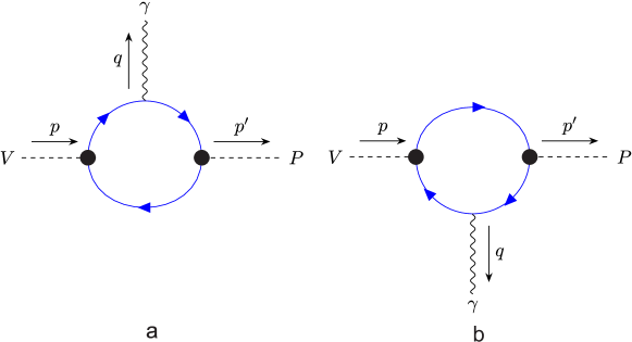
Figure 1: Feynman diagrams describing the radiative decays of a vector meson.

One has to note that there is an additional piece in the Lagrangian related to the gauging nonlocal interactions of hadrons with their constituents Branz:2009cd . This piece gives the additional contributions to the electromagnetic processes. However, they are identically zero for the process $V\to P\gamma$ due to its anomalous nature.

The matrix element of the process $V\to P\gamma$ is written down

$$M_{VP\gamma}(p;p^{\prime},q)=eg_{V}g_{P}\epsilon^{V}_{\nu}(p)\epsilon^{\gamma}_{\mu}(q)\int\!\!dx\!\!\int\!\!dy\!\!\int\!\!dz\,e^{-ipx+ip^{\prime}y+iqz}\langle\,T\{\bar{J}_{V}^{\nu}(x)J^{\mu}_{\rm em}(z)J_{P}(y)\}\rangle_{0}.$$ (13)

Using the Fourier transforms of the quark currents, we come to the final result

$$M_{VP\gamma}(p;p^{\prime},q) = (2\pi)^{4}i\,\delta(p-p^{\prime}-q)M(p,p^{\prime}),$$

$$M(p,p^{\prime}) = (-3i)eg_{V}g_{P}\epsilon^{V}_{\nu}(p)\epsilon^{\gamma}_{\mu}(q)\,\left(e_{b}M^{\mu\nu}_{b}+e_{q}M^{\mu\nu}_{q}\right)$$

$$M^{\mu\nu}_{b} = \int\!\!\frac{dk}{(2\pi)^{4}i}\widetilde{\Phi}_{V}(-\ell_{1}^{2})\widetilde{\Phi}_{P}(-\ell_{2}^{2})\mbox{\rm{tr}}\left[S_{q}(k)\gamma^{\nu}S_{b}(k-p)\gamma^{\mu}S_{b}(k-p^{\prime})\gamma^{5}\right]$$

$$M^{\mu\nu}_{q} = \int\!\!\frac{dk}{(2\pi)^{4}i}\widetilde{\Phi}_{V}(-\ell_{3}^{2})\widetilde{\Phi}_{P}(-\ell_{4}^{2})\mbox{\rm{tr}}\left[S_{q}(k+p^{\prime})\gamma^{\mu}S_{q}(k+p)\gamma^{\nu}S_{b}(k)\gamma^{5}\right]$$ (14)

where $\ell_{1}=k-w_{2}\,p$, $\ell_{2}=k-w_{2}\,p^{\prime}$ and $\ell_{3}=k+w_{1}\,p$, $\ell_{2}=k+w_{1}\,p^{\prime}$. The ratios of quark masses are defined by Eq. (4). Now one has $m_{q_{1}}=m_{b}$ and $m_{q_{2}}=m_{q}$ with $q=u,d,s$. By using the technique of calculations outlined in Sec. II and taking into account the transversality conditions $\epsilon^{\gamma}_{\mu}(q)q^{\mu}=0$ and $\epsilon^{V}_{\nu}(p)p^{\nu}=0$ one can arrives at the standard form of matrix element

$$M(p,p^{\prime})=e\,g_{VP\gamma}\,\varepsilon^{pq\mu\nu}\epsilon^{\gamma}_{\mu}(q)\epsilon^{V}_{\nu}(p),$$ (15)

where $g_{VP\gamma}=e_{b}I_{b}(m^{2}_{V},m^{2}_{P})+e_{q}I_{q}(m^{2}_{V},m^{2}_{P})$ is radiative decay constant. The quantities $I_{b,q}$ are defined by the two-fold integrals which are calculated numerically. The electromagnetic decay width is written as

$$\Gamma(V\to P+\gamma)=\frac{\alpha}{24}m_{V}^{3}\left(1-\frac{m_{P}^{2}}{m_{V}^{2}}\right)^{3}g_{VP\gamma}^{2}\,.$$ (16)

III.2 $V\to P\gamma$: numerical results

The masses of the $B^{\ast}$-meson family is not well established yet. We collect the experimentally measured masses of $B$-meson family in Table 2

Table 2: Masses of $B$-meson family taken from PDG ParticleDataGroup:2022pth (in MeV).

$B^{\pm}$	$B^{0}$	$B^{0}_{s}$	$B^{+}_{c}$	$B^{\ast}$	$B^{\ast}_{s}$
5279.25(26)	5279.63(20)	5366.91(11)	6274.47(32)	5324.71(21)	5415.8(1.5)

Since the $B_{c}^{\ast}$ or $B_{c}(1^{3}S_{1})$ state has not been observed yet, we will use the value $m(B_{c}^{\ast})~{}=~{}6331(4)(6)$ MeV obtained from lattice QCD Mathur:2018epb . The values of size parameters are taken from our previous papers Dubnicka:2017job ; Gutsche:2018utw ; Ivanov:2019nqd . Their numerical values are given in Table 3.

Table 3: Size parameters of $B$-meson family (in GeV).

$\Lambda_{B}$	$\Lambda_{B_{s}}$	$\Lambda_{B_{c}}$	$\Lambda_{B^{\ast}}$	$\Lambda_{B^{\ast}_{s}}$	$\Lambda_{B^{\ast}_{c}}$
1.96	2.05	2.73	1.72	1.71	2.42

The numerical results for the radiative decay constants are shown in Table 4. They are compared with those obtained in Ref. Li:2020rcg .

Table 4: The numerical results for the radiative decay constants (in GeV).

$g_{B^{\ast\,+}B^{+}\gamma}$	$g_{B^{\ast\,0}B^{0}\gamma}$	$g_{B_{s}^{\ast\,0}B_{s}^{0}\gamma}$	$g_{B_{c}^{\ast\,+}B_{c}^{+}\gamma}$	Ref.
1.28(13)	-0.76(8)	-0.57(6)	0.28(3)	CCQM
1.44	-0.91	-0.74	—	Li:2020rcg

The numerical values for the radiative decay widths are given in Tables 5 and 6. Our findings are compared with the results obtained in other approaches.

Now, we briefly discuss some error estimates within our model. The CCQM consists of several free parameters: the constituent quark masses $m_{q}$, the hadron size parameters $\Lambda_{H}$ and the universal infrared cutoff parameter $\lambda$. These parameters are determined by minimizing the functional $\chi^{2}=\sum\limits_{i}\frac{(y_{i}^{\rm expt}-y_{i}^{\rm theor})^{2}}{\sigma^{2}_{i}}$ where $\sigma_{i}$ is the experimental uncertainty. If $\sigma$ is too small then we take its value of 10$\%$. Besides, we have observed that the errors of the fitted parameters are of the order of 10$\%$. Thus, the theoretical error of the CCQM is estimated to be of the order of 10$\%$ at the level of matrix elements and the order of 15$\%$ at the level of widths.

Table 5: Widths of $B^{\ast}\to B\gamma$ and $B_{s}^{\ast}\to B_{s}\gamma$ decays (in eV).

Mode	CCQM	Chang:2019xtj	Choi:2007se	Ebert:2002xz	Goity:2000dk	Zhu:1996qy	Ivanov:1994ji	Colangelo:1993zq
$B^{\ast+}\to B^{+}\gamma$	372(56)	349(18)	400(30)	190	740(88)	380(60)	401	220(90)
$B^{\ast\,0}\to B^{0}\gamma$	126(19)	116(6)	130(10)	70	228(27)	130(30)	131	75(27)
$B_{s}^{\ast\,0}\to B_{s}^{0}\gamma$	90(14)	84(10)	68(17)	54	136(12)	220(40)

Table 6: Widths of $B_{c}^{\ast}\to B_{c}\gamma$ decay (in eV).

Mode	CCQM	Liu:2022bdq	Godfrey:2004ya	Fulcher:1998ka	Ebert:2002xz	Gershtein:1994dxw	Eichten:1994gt
$B_{c}^{\ast\,+}\to B_{c}^{+}\gamma$	33(5)	53(3)	80	59	33	60	135

As can be seen from the Table 5, there is suppression of the neutral mode $B^{\ast\,0}\to B^{0}\gamma$ compared to the charged mode $B^{\ast+}\to B^{+}\gamma$. The ratio of those widths is written as

$$\frac{\Gamma(B^{\ast\,0}\to B^{0}\gamma)}{\Gamma(B^{\ast+}\to B^{+}\gamma)}\sim\frac{(I_{b}+I_{d})^{2}}{{(I_{b}-2I_{u})^{2}}}\approx 0.38.$$ (17)

Note that in the heavy quark limit $m_{b}\to\infty$ the integral $I_{b}$ is suppressed as $1/m_{b}$ compare with $I_{q}$ $(q=u,d)$. Therefore our result for the ratio in Eq. (17) is not far from the the heavy quark limit $0.25$. This confirms the observation that the heavy quark limit is quite reliable in the case of $b$-quark.

IV Nonleptonic decays

The effective Hamiltonian describing the nonleptonic decays $B^{\ast}_{u,d,s}\to D^{\ast}_{u,d,s}\,+\,V$ where $V=D^{\ast}_{u,d,s},K^{\ast}_{u,d},\rho$ is written down

$$\mbox{${\cal H}_{\rm eff}$}=-\frac{G_{F}}{\sqrt{2}}V^{\ast}_{cb}V_{q_{1}q_{2}}\Big{(}C_{2}\left(\bar{c}_{a}O^{\mu}b_{a}\right)\left(\bar{q}_{1b}O_{\mu}q_{2b}\right)+C_{1}\left(\bar{c}_{a}O^{\mu}b_{b}\right)\left(\bar{q}_{1b}O_{\mu}q_{2a}\right)\Big{)}$$ (18)

where $G_{F}$ is the Fermi constant, $V_{cb}$ and $V_{q_{1}q_{2}}$ are the matrix elements of the CKM-matrix, $C_{1}$ and $C_{2}$ is Wilson coefficients and $O^{\mu}=\gamma^{\mu}(1-\gamma_{5})$ is the weak matrix with the left chirality. The Wilson coefficients $C_{2}$ (leading order) and $C_{1}$ (subleading order) are taken at the scale of $b$-quark mass from Ref. Descotes-Genon:2013vna (see, Table 3). One has

$$C_{1}=-0.2632\qquad\text{and}\qquad C_{2}=1.0111.$$ (19)

One has to emphasize that if QCD is neglected, than $C_{1}=0$ and $C_{2}=1$ Buchalla:1995vs ; Buras:1998raa .

We consider the nonleptonic decays $B^{\ast}\to D^{\ast}V$ which proceed via tree-level quark diagrams shown in Fig. 2. One has to note that the Wilson coefficients will appear in combinations either $a_{1}=C_{2}+\xi C_{1}$ for the charged emitted meson or $a_{2}=C_{1}+\xi C_{2}$ for the neutral emitted meson. The color suppression factor $\xi=1/N_{c}$ will be used to be equal to zero in calculation that corresponds to the large-$N_{c}$ limit $\xi=0$. One has to remind that an approximation is widely used in the phenomenological studies of two-body nonleptonic decays because in the case of $N_{c}=3$ the combination $a_{2}\approx 0.074$, i.e. significantly suppressed.

Figure 2: Tree-level quark diagrams

The Feynman diagram describing the nonleptonic decays $B^{\ast}\to M_{1}M_{2}$ within the CCQM are shown in Fig. 3.

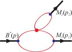
Figure 3: Diagram describing the nonleptonic decay $B^{\ast}\to M_{1}M_{2}$.

The matrix element of the nonleptonic $B^{\ast}\to M_{1}(p_{1})M_{2}(p_{2})$ decays are given by

$$M(B^{\ast}(p)\to M_{1}(p_{1})M_{2}(p_{2})) = \frac{G_{F}}{\sqrt{2}}V_{CKM}a_{W}\,m_{2}f_{M_{2}}\epsilon_{2\,\mu}\,$$ (20)

$$\times \Big{\langle}M_{1}\left(p_{1},\epsilon_{1\,\beta}\right)|\bar{q}_{1}O^{\mu}q_{2}|B^{\ast}(p,\epsilon^{\ast}_{\alpha})\Big{\rangle}$$

where $f_{M_{2}}$ is the leptonic decay constant of the vector meson $M_{2}$. Here $V_{CKM}$ and $a_{W}$ are the relevant CKM-matrix elements and the Wilson coefficients, respectively. Note that the Eq. (20) is equivalent to the factorization hypothesis.

The leptonic decay constant of the vector meson $M_{2}$ which consists from $q_{1}$ and $q_{2}$ quarks is defined by

$$N_{c}\,g_{M_{2}}\!\int\!\!\frac{d^{4}k}{(2\pi)^{4}i}\,\widetilde{\Phi}_{M_{2}}(-k^{2})\,\mbox{\rm{tr}}\biggl{[}O^{\,\mu}S_{1}(k+w_{1}p_{2})\not\!\epsilon_{2}S_{2}(k-w_{2}p_{2})\biggr{]}=m_{2}f_{M_{2}}\epsilon_{2}^{\mu}.$$ (21)

The meson is taken on its mass-shell, i.e. $p_{2}^{2}=m^{2}_{2}$ and $\epsilon_{2}\cdot p_{2}=0$.

The matrix elements of the weak $B^{\ast}-M_{1}$ transition is written as

$$\langle M_{1}(p_{1})|\bar{q}_{1}O^{\mu}q_{2}|B^{\ast}(p)\rangle=$$

$$=N_{c}\,g_{B^{\ast}}\,g_{M_{1}}\epsilon_{\alpha}(p)\epsilon^{\ast}_{1\,\beta}(p_{1})\!\!\int\!\!\frac{d^{4}k}{(2\pi)^{4}i}\,\widetilde{\Phi}_{B^{\ast}}\Big{(}-(k+w_{13}p_{1})^{2}\Big{)}\,\widetilde{\Phi}_{M_{1}}\Big{(}-(k+w_{23}p_{2})^{2}\Big{)}$$

$$\times\mbox{\rm{tr}}\biggl{[}O^{\,\mu}\,S_{1}(k+p_{1})\,\gamma^{\alpha}\,S_{3}(k)\,\gamma^{\beta}\,S_{2}(k+p_{2})\biggr{]}.$$ (22)

All particles are on their mass shell: $p^{2}=m^{2}_{B^{\ast}}$, $\epsilon_{\alpha}\,p^{\alpha}=0$, and $p_{1}^{2}=m^{2}_{1}$, $\epsilon_{1\,\beta}\,p_{1}^{\beta}=0$. Altogether there are three flavors of quarks involved in this process. We therefore introduce a notation with two subscripts $w_{ij}=m_{q_{j}}/(m_{q_{i}}+m_{q_{j}})$ $(i,j=1,2,3)$ such that $w_{ij}+w_{ji}=1$. The loop integrations in the Eqs. (21) and (22) are performed by using technique given in Sec. II. We finalize by two- and three-fold integrals in equations Eqs. (21) and (22), respectively. We calculate them by using FORTRAN codes with NAG library.

The matrix elements of the weak $B^{\ast}-M_{1}$ transition can be expressed in terms of six vector form factors $V_{i}$ and four axial form factors $A_{i}$. One has

$$\langle M_{1}(p_{1})|\bar{q}_{1} O^{\mu}q_{2}|B^{\ast}(p)\rangle=\epsilon_{\alpha}\epsilon^{\ast}_{1\,\beta}\times\Big{[}g^{\alpha\beta}\left(-P^{\mu}V_{1}(q^{2})+q^{\mu}V_{2}(q^{2})\right)$$

$$+\frac{q^{\alpha}q^{\beta}}{M^{2}-m^{2}_{1}}\left(P^{\mu}V_{3}(q^{2})-q^{\mu}V_{4}(q^{2})\right)-q^{\alpha}g^{\mu\beta}V_{5}(q^{2})+q^{\beta}g^{\mu\alpha}V_{6}(q^{2})\Big{]}$$

$$+\epsilon_{\alpha}\epsilon^{\ast}_{1\,\beta}\times\Big{[}-i\varepsilon^{\mu\nu\alpha\beta}\left(P^{\nu}A_{1}(q^{2})-q^{\nu}A_{2}(q^{2})\right)$$

$$+\frac{i\varepsilon^{\mu\nu qP}}{M^{2}-m^{2}_{1}}\left(g^{\nu\alpha}q^{\beta}A_{3}(q^{2})-g^{\nu\beta}q^{\alpha}A_{4}(q^{2})\right)\Big{]}$$ (23)

where $P=p+p_{1}$, $q=p-p_{1}=p_{2}$. The full matrix element of the nonleptonic decay $B^{\ast}(p)\to M_{1}(p_{1})M_{2}(p_{2})$ is obtained by contraction of the above two expressions from Eqs. (21) and (23). Keeping in mind that $\epsilon^{\ast}_{2}\cdot q=(\epsilon^{\ast}_{2}\cdot p_{2})=0$ one gets that the two vector form factors $V_{2}$ and $V_{4}$ do not contribute to the full matrix element.

The values of the size parameters of vector mesons are taken from Ref. Dubnicka:2017job ; Gutsche:2018utw ; Ivanov:2019nqd and displayed in Table 7.

Table 7: Size parameters of vector mesons (in GeV)

$\Lambda_{\rho}$	$\Lambda_{K^{\ast}}$	$\Lambda_{D^{\ast}}$	$\Lambda_{D^{\ast}_{s}}$	$\Lambda_{B^{\ast}}$	$\Lambda_{B^{\ast}_{s}}$
0.61	0.81	1.53	1.56	1.72	1.71

The calculated leptonic decay constants $f_{M_{2}}$ are shown in Table 8.

Table 8: Calculated leptonic decay constants $f_{M_{2}}$ (in MeV)

	CCQM	Expt/Lat
$f_{\rho}$	218(22)	$221(1)\quad$  ParticleDataGroup:2022pth
$f_{K^{\ast}}$	227(23)	$217(7)\quad$  ParticleDataGroup:2022pth
$f_{D^{\ast}}$	246(25)	$223.5(8.4)$ Lubicz:2017asp
$f_{D^{\ast}_{s}}$	273(27)	$268.8(6.6)$ Lubicz:2017asp
$f_{B^{\ast}}$	185(19)	$186.4(7.1)$ Lubicz:2017asp ; ETM:2016nbo
$f_{B^{\ast}_{s}}$	260(26)	$223.1(5.6)$ Lubicz:2017asp ; ETM:2016nbo

We calculate the relevant transition form factors in the full kinematical region of the transfered momentum squared $q^{2}$. The behavior of the form factors on the $q^{2}$ are shown in Figs. 4-7.

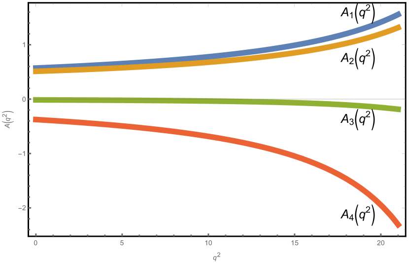
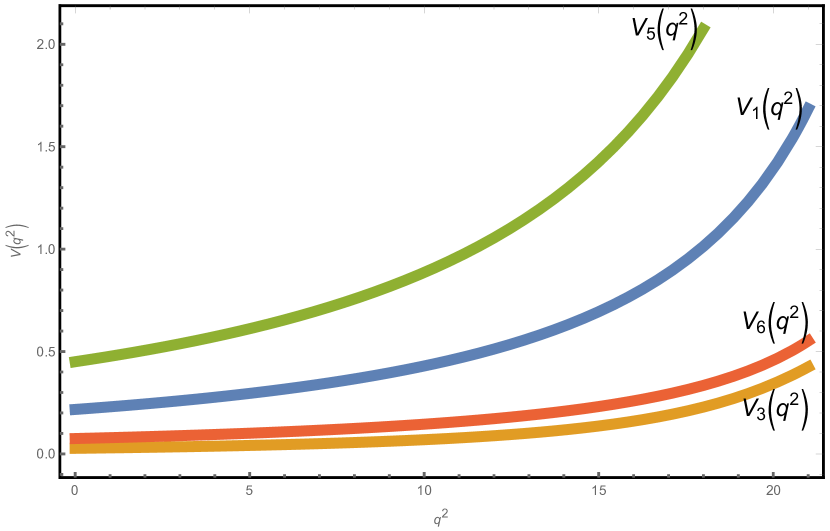
Figure 4: Form factors of $B^{\ast}-\rho$ transition

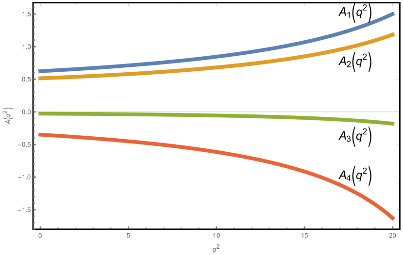
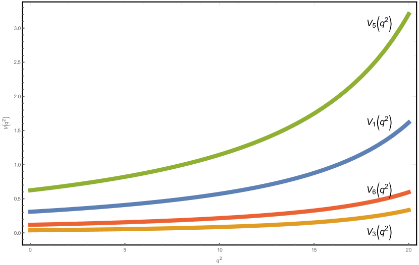
Figure 5: Form factors of $B^{\ast}-K^{\ast}$ transition

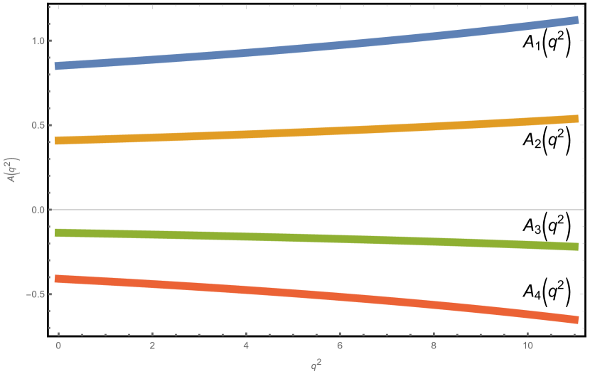
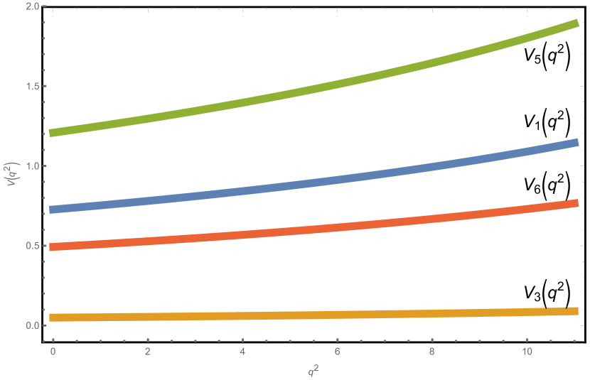
Figure 6: Form factors of $B^{\ast}-D^{\ast}$ transition

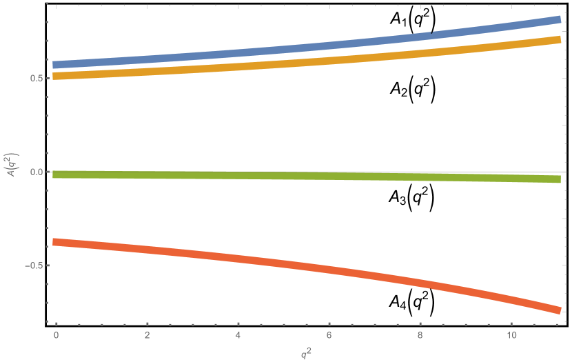
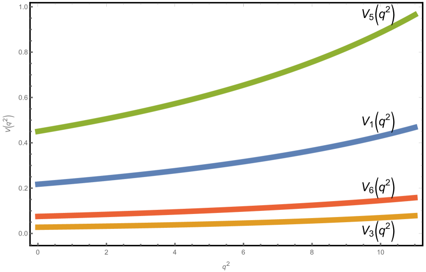
Figure 7: Form factors of $B_{s}^{\ast}-D_{s}^{\ast}$ transition

The numerical results for the form factors are well approximated by a dipole parametrization

$$F(q^{2})=\frac{F(0)}{1-as+bs^{2}},\qquad s=\frac{q^{2}}{M^{2}}$$ (24)

where $M$ is the mass of ingoing meson. The dipole approximation is quite accurate. The error relative to the exact results is less than 1$\%$ over the entire $q^{2}$ range.

Table 9: Parameters of dipole approximation

$B^{\ast}-\rho$	$A_{1}$	$A_{2}$	$A_{3}$	$A_{4}$	$V_{1}$	$V_{3}$	$V_{5}$	$V_{6}$
F(0)	0.57	0.51	$-0.014$	$-0.38$	0.22	0.027	0.45	0.075
a	0.66	0.58	2.08	1.42	1.61	2.13	1.59	1.55
b	$-0.26$	$-0.33$	1.13	0.39	0.58	1.17	0.57	0.52

$B^{\ast}-K^{\ast}$	$A_{1}$	$A_{2}$	$A_{3}$	$A_{4}$	$V_{1}$	$V_{3}$	$V_{5}$	$V_{6}$
F(0)	$0.62$	$0.51$	$-0.027$	$-0.35$	$0.31$	$0.038$	$0.62$	$0.12$
a	$0.66$	$0.59$	$1.75$	$1.34$	$1.46$	$1.92$	$1.44$	$1.42$
b	$-0.24$	$-0.31$	$0.77$	$0.31$	$0.44$	$0.94$	$0.42$	$0.40$

$B^{\ast}-D^{\ast}$	$A_{1}$	$A_{2}$	$A_{3}$	$A_{4}$	$V_{1}$	$V_{3}$	$V_{5}$	$V_{6}\qquad$
F(0)	0.85	0.41	$-0.14$	$-0.41$	0.73	0.050	1.21	0.49
a	0.57	0.56	1.02	1.01	0.98	1.29	0.97	0.95
b	$-0.14$	$-0.15$	0.14	0.13	$0.11$	0.36	0.10	0.089

$B_{s}^{\ast}-D_{s}^{\ast}$	$A_{1}$	$A_{2}$	$A_{3}$	$A_{4}$	$V_{1}$	$V_{3}$	$V_{5}$	$V_{6}\qquad$
F(0)	0.78	0.38	$-0.11$	$-0.34$	0.68	0.051	1.16	0.49
a	0.71	0.69	1.16	1.11	1.10	1.36	1.08	1.07
b	$-0.13$	$-0.16$	0.21	0.15	$0.15$	0.38	0.15	0.13

Table 10: Form factors at origin $q^{2}=0$ compared with CLFQM Chang:2019xtj

$B^{\ast}-\rho$	CCQM	CLFQM
$A_{1}$	0.57	0.27
$A_{2}$	0.51	0.25
$A_{3}$	-0.014	0.07
$A_{4}$	-0.38	0.06
$V_{1}$	0.22	0.28
$V_{3}$	0.027	0.11
$V_{5}$	0.45	0.60
$V_{6}$	0.075	0.14

$B^{\ast}-K^{\ast}$	CCQM	CLFQM
$A_{1}$	0.62	0.33
$A_{2}$	0.51	0.27
$A_{3}$	-0.027	0.07
$A_{4}$	-0.35	0.07
$V_{1}$	0.31	0.33
$V_{3}$	0.038	0.11
$V_{5}$	0.62	0.68
$V_{6}$	0.12	0.16

$B^{\ast}-D^{\ast}$	CCQM	CLFQM
$A_{1}$	0.85	0.66
$A_{2}$	0.41	0.35
$A_{3}$	-0.14	0.07
$A_{4}$	-0.41	0.08
$V_{1}$	0.73	0.67
$V_{3}$	0.050	0.13
$V_{5}$	1.21	1.17
$V_{6}$	0.49	0.48

$B^{\ast}_{s}\to D^{\ast}_{s}$	CCQM	CLFQM
$A_{1}$	0.78	0.65
$A_{2}$	0.38	0.38
$A_{3}$	-0.11	0.10
$A_{4}$	-0.34	0.09
$V_{1}$	0.68	0.66
$V_{3}$	0.051	0.15
$V_{5}$	1.16	1.19
$V_{6}$	0.49	0.53

For convenience of calculation, we further introduce the helicity amplitudes $H^{M_{1}M_{2}}_{\lambda_{1}\lambda_{2}}$ for the outgoing mesons $M_{1}$ and $M_{2}$. We imply that the meson $M_{2}$ is the emitted meson whereas $M_{1}$ is the outgoing meson in the transition $B^{\ast}-M_{1}$. One has

$$H^{M_{1}M_{2}}_{00}=f_{M_{2}}m_{2} \Big{[}+\frac{|\mathbf{p_{2}}|\left(M^{2}+m_{1}^{2}-m_{2}^{2}\right)}{m_{1}m_{2}}V_{1}+\frac{2M^{2}|\mathbf{p_{2}}|^{3}}{\left(M^{2}-m_{1}^{2}\right)m_{1}m_{2}}V_{3}$$

$$\,\,-\frac{|\mathbf{p_{2}}|\left(M^{2}-m_{1}^{2}-m_{2}^{2}\right)}{2m_{1}m_{2}}V_{5}+\frac{|\mathbf{p_{2}}|\left(M^{2}-m_{1}^{2}+m_{2}^{2}\right)}{2m_{1}m_{2}}V_{6}\Big{]}\,,$$

$$H^{M_{1}M_{2}}_{++}=f_{M_{2}}m_{2} \Big{[}+\frac{3M^{2}+m_{1}^{2}-m_{2}^{2}}{2M}A_{1}-\frac{M^{2}-m_{1}^{2}+m_{2}^{2}}{2M}A_{2}+\frac{2|\mathbf{p_{2}}|^{2}M}{M^{2}-m_{1}^{2}}A_{4}-|\mathbf{p_{2}}|V_{5}\Big{]}\,,$$

$$H^{M_{1}M_{2}}_{--}=f_{M_{2}}m_{2} \Big{[}-\frac{3M^{2}+m_{1}^{2}-m_{2}^{2}}{2M}A_{1}+\frac{M^{2}-m_{1}^{2}+m_{2}^{2}}{2M}A_{2}-\frac{2|\mathbf{p_{2}}|^{2}M}{M^{2}-m_{1}^{2}}A_{4}-|\mathbf{p_{2}}|V_{5}\Big{]}\,,$$

$$H^{M_{1}M_{2}}_{+0}=f_{M_{2}}m_{2} \Big{[}-\frac{M^{2}-m_{1}^{2}}{m_{2}}A_{1}+m_{2}A_{2}+\frac{2M|\mathbf{p_{2}}|}{m_{2}}V_{1}\Big{]}\,,$$

$$H^{M_{1}M_{2}}_{-0}=f_{M_{2}}m_{2} \Big{[}+\frac{M^{2}-m_{1}^{2}}{m_{2}}A_{1}-m_{2}A_{2}+\frac{2M|\mathbf{p_{2}}|}{m_{2}}V_{1}\Big{]}\,,$$

$$H^{M_{1}M_{2}}_{0-}=f_{M_{2}}m_{2} \Big{[}-\frac{M^{2}+3m_{1}^{2}-m_{2}^{2}}{2m_{1}}A_{1}+\frac{M^{2}-m_{1}^{2}-m_{2}^{2}}{2m_{1}}A_{2}-\frac{2|\mathbf{p_{2}}|^{2}M^{2}}{\left(M^{2}-m_{1}^{2}\right)m_{1}}A_{3}$$

$$\,\,-\frac{M|\mathbf{p_{2}}|}{m_{1}}V_{6}\Big{]}\,,$$

$$H^{M_{1}M_{2}}_{0+}=f_{M_{2}}m_{2} \Big{[}+\frac{M^{2}+3m_{1}^{2}-m_{2}^{2}}{2m_{1}}A_{1}-\frac{M^{2}-m_{1}^{2}-m_{2}^{2}}{2m_{1}}A_{2}+\frac{2|\mathbf{p_{2}}|^{2}M^{2}}{\left(M^{2}-m_{1}^{2}\right)m_{1}}A_{3}$$

$$\,\,-\frac{M|\mathbf{p_{2}}|}{m_{1}}V_{6}\Big{]}\,.$$

Here $|\mathbf{p_{2}}|=\lambda^{1/2}(M^{2},m_{1}^{2},m_{2}^{2})/2M$ is the momentum of the daughter meson in the $B^{\ast}$-meson rest frame.

Finally, the amplitudes can be written in terms of helicity amplitudes. The only two amplitudes contain the contributions from the diagrams with the charged and neutral emitted mesons. They are written as

$$M(B^{\ast-}\to D^{\ast 0}+K^{\ast-}) = \frac{G_{F}}{\sqrt{2}}\Big{(}a_{1}V_{cb}V^{\ast}_{us}H_{\lambda_{D^{\ast}}\lambda_{K^{\ast}}}^{D^{\ast}K^{\ast}}+a_{2}V_{cb}V^{\ast}_{us}H_{\lambda_{K^{\ast}}\lambda_{D^{\ast}}}^{K^{\ast}D^{\ast}}\Big{)},$$

$$M(B^{*-}\to D^{*0}+\rho^{-}) = \frac{G_{F}}{\sqrt{2}}\Big{(}a_{1}V_{cb}V^{\ast}_{ud}H_{\lambda_{D^{\ast}}\lambda_{\rho}}^{D^{\ast}\rho}+a_{2}V_{cb}V^{\ast}_{ud}H_{\lambda_{\rho}\lambda_{D^{\ast}}}^{\rho D^{\ast}}\Big{)}.$$ (25)

Other ten amplitudes contain the contributions from the diagrams with the charged emitted mesons only. One has

Table 11: Amplitudes of $B^{\ast}\to D^{\ast}V_{\rm charge}$ decays.

$M(B^{\ast}\to D^{\ast}V_{\rm charge})={\bf\frac{G_{F}}{\sqrt{2}}a_{1}V_{cb}}\,\widetilde{M}(B^{\ast}\to D^{\ast}V_{\rm charge})$
Mode	$\widetilde{M}$	Mode	$\widetilde{M}$
$B^{*-}\to D^{*0}\,D^{*-}$	$V^{\ast}_{cd}\,H_{\lambda_{D^{\ast 0}}\lambda_{D^{\ast-}}}^{D^{\ast 0}D^{\ast-}}$	$B^{*-}\to D^{*0}\,D^{*-}_{s}$	$V^{\ast}_{cs}\,H_{\lambda_{D^{\ast}}\lambda_{D_{s}^{\ast}}}^{D^{\ast}D^{\ast}_{s}}$
$\bar{B}^{*0}\to D^{*+}\,K^{*-}$	$V^{\ast}_{us}\,H_{\lambda_{D^{\ast}}\lambda_{K^{\ast}}}^{D^{\ast}K^{\ast}}$	$\bar{B}^{*0}\to D^{*+}\,\rho^{-}$	$V^{\ast}_{ud}\,H_{\lambda_{D^{\ast}}\lambda_{\rho}}^{D^{\ast}\rho}$
$\bar{B}^{*0}\to D^{*+}\,D^{*-}$	$V^{\ast}_{cd}\,H_{\lambda_{D^{\ast+}}\lambda_{D^{\ast-}}}^{D^{\ast+}D^{\ast-}}$	$\bar{B}^{*0}\to D^{*+}\,D_{s}^{*-}$	$V^{\ast}_{cs}H_{\lambda_{D^{\ast}}\lambda_{D^{\ast}_{s}}}^{D^{\ast}D^{\ast}_{s}}$
$\bar{B}_{s}^{*0}\to D^{*+}_{s}\,K^{*-}$	$V^{\ast}_{us}\,H_{\lambda_{D_{s}^{\ast}}\lambda_{K^{\ast}}}^{D^{\ast}_{s}K^{\ast}}$	$\bar{B}_{s}^{*0}\to D^{*+}_{s}\,\rho^{-}$	$V^{\ast}_{ud}\,H_{\lambda_{D_{s}^{\ast}}\lambda_{\rho}}^{D^{\ast}_{s}\rho}$
$\bar{B}_{s}^{*0}\to D^{*+}_{s}\,D^{\ast-}$	$V^{\ast}_{cd}\,H_{\lambda_{D_{s}^{\ast}}\lambda_{D^{\ast}}}^{D^{\ast}_{s}D^{\ast}}$	$\bar{B}_{s}^{*0}\to D^{*+}_{s}\,D^{\ast-}_{s}$	$V^{\ast}_{cs}\,H_{\lambda_{D_{s}^{\ast+}}\lambda_{D_{s}^{\ast-}}}^{D^{\ast+}_{s}D^{\ast-}_{s}}$

By assuming that the $B^{\ast}$-meson is unpolarized, the decay widths are calculated by the formulas

$$\Gamma\left(B^{\ast\,\lambda}\to M_{1}^{\lambda_{1}}M_{2}^{\lambda_{2}}\right)=\frac{|\mathbf{p_{2}}|}{24\pi\,M^{2}}\sum\limits_{\lambda_{1}\lambda_{2}}|M(B^{\ast}\to M_{1}M_{2})|^{2}$$ (26)

where $\lambda=-\lambda_{1}+\lambda_{2}$. In Table 12 the branching fractions of all weak nonleptonic decays considered here are given. As wide accepted, we used the calculated values of the radiative decay widths as total widths, i.e. $\Gamma_{\rm tot}(B^{\ast})=\Gamma(B^{\ast}\to B\gamma$). For comparison, we give the results obtained in Ref. Chang:2019xtj .

Table 12: Branching fractions of the $B^{\ast}\to D^{\ast}V$ decays ($V=\rho,K^{\ast},D^{\ast},D_{s}^{\ast}$)

Decay mode	CCQM	CLFQM Chang:2019xtj
$B^{*-}\to D^{*0}+K^{*-}$	$1.02(15)\times 10^{-9}$	$1.10^{+0.01+0.19}_{-0.01-0.17}\times 10^{-11}$
$B^{*-}\to D^{*0}+\rho^{-}$	$1.92(29)\times 10^{-8}$	$2.23^{+0.04+0.39}_{-0.04-0.35}\times 10^{-10}$
$B^{*-}\to D^{*0}+D^{*-}$	$1.75(26)\times 10^{-9}$	$1.44^{+0.11+0.24}_{-0.11-0.22}\times 10^{-11}$
$B^{*-}\to D^{*0}+D^{*-}_{s}$	$3.85(58)\times 10^{-8}$	$3.71^{+0.18+0.64}_{-0.18-0.57}\times 10^{-10}$
$\bar{B}^{*0}\to D^{*+}+K^{*-}$	$4.62(69)\times 10^{-9}$	$3.40^{+0.24+0.58}_{-0.23-0.52}\times 10^{-11}$
$\bar{B}^{*0}\to D^{*+}+\rho^{-}$	$8.09(1.21)\times 10^{-8}$	$6.85^{+0.26+1.17}_{-0.26-1.05}\times 10^{-10}$
$\bar{B}^{*0}\to D^{*+}+D^{*-}$	$5.12(77)\times 10^{-9}$	$4.33^{+0.33+0.74}_{-0.32-0.66}\times 10^{-11}$
$\bar{B}^{*0}\to D^{*+}+D^{*-}_{s}$	$1.17(18)\times 10^{-7}$	$1.11^{+0.06+0.19}_{-0.05-0.17}\times 10^{-9}$
$\bar{B}^{*0}_{s}\to D^{*+}_{s}+K^{*-}$	$5.63(84)\times 10^{-9}$	$4.80^{+0.34+0.83}_{-0.32-0.74}\times 10^{-11}$
$\bar{B}^{*0}_{s}\to D^{*+}_{s}+\rho^{-}$	$5.21(78)\times 10^{-9}$	$9.39^{+0.36+1.63}_{-0.35-1.46}\times 10^{-10}$
$\bar{B}^{*0}_{s}\to D^{*+}_{s}+D^{*-}$	$6.51(98)\times 10^{-9}$	$6.10^{+0.47+1.03}_{-0.45-0.92}\times 10^{-11}$
$\bar{B}^{*0}_{s}\to D^{*+}_{s}+D^{*-}_{s}$	$1.48(22)\times 10^{-7}$	$1.54^{+0.08+0.26}_{-0.07-0.24}\times 10^{-9}$

One can see from Table 12 that our results are almost two order larger in magnitude than those from Ref. Chang:2019xtj . Unfortunately, the authors of Chang:2019xtj did not give the numerical coefficients for the Wilson coefficients $C_{1}$ and $C_{2}$, there are only the combinations of $\alpha_{1}=C_{1}+\xi C_{2}$ and $\alpha_{2}=C_{2}+\xi C_{1}$ with $\xi=1/N_{c}$. However, they refer to the papers by Buras et al. Buchalla:1995vs ; Buras:1998raa in which the notation are accepted as $C_{2}=1$ and $C_{1}=0$ if QCD is neglected. We are using the Wilson coefficients from Ref. Descotes-Genon:2013vna (see, Table 3, and references therein) where their values have been calculated by using the various corrections and found that $C_{1}=-0.2632$ and $C_{2}=1.0111$. If one uses these values for $\alpha_{1}$ and $\alpha_{2}$ of Ref. Chang:2019xtj then one arrives at $\alpha_{1}\approx 0.074$ for $N_{c}=3$, i.e. strongly suppressed, whereas the value of $\alpha_{2}=0.923$ is of the leading order. If compare the analytical expressions for the decay amplitudes from Chang:2019xtj (see, Eqs. (13)-(24)) with our results given by Eq. 25 and Table 11, then one finds that in Ref. Chang:2019xtj the amplitudes with the charged emitted mesons are proportinal to $\alpha_{1}$ which is suppressed whereas in our approach those amplitudes are proportinal to $a_{1}=C_{2}+\xi C_{1}$ which is of leading order. It could explain two order difference for branching fractions obtained in these two approaches.

V Summary

The radiative and weak nonleptonic decays of vector $B$-mesons have been studied within the covariant confined quark model (CCQM) developed in our previous papers. The matrix elements and decays widths of the radiative decays $B^{\ast}\to B\gamma$ were calculated. The obtained results were compared with those obtained in other approaches.

The nonleptonic decays $B^{\ast}\to D^{\ast}V$ which proceed via tree-level quark diagrams have been carefully analized. It was shown that the analytical expressions for the amplitudes correspond to the factorization approach. In the framework of our approach we calculated the leptonic decay constants and the form factors of the $B^{\ast}\to D^{\ast}(V)$ transitions in the entire physical region of the momentum transfer squared. Finally, we calculated the two-body decay widths and compared our results with other models.

VI Acknowledgements

This work is supported by the JINR grant of young scientists and specialists No. 22-302-06. Zh.T.’s research has been funded by the Science Committee of the Ministry of Education and Science of the Republic of Kazakhstan (Grant No. AP09057862).

References

- (1) R. Louvot et al. [Belle], Phys. Rev. Lett. 102, 021801 (2009) [arXiv:0809.2526 [hep-ex]].
- (2) R. Aaij et al. [LHCb], Phys. Rev. Lett. 110, no.15, 151803 (2013) [arXiv:1211.5994 [hep-ex]].
- (3) G. Aad et al. [ATLAS], Phys. Rev. Lett. 113, no.21, 212004 (2014) [arXiv:1407.1032 [hep-ex]].
- (4) R. Aaij et al. [LHCb], JHEP 01, 138 (2018) [arXiv:1712.04094 [hep-ex]].
- (5) A. M. Sirunyan et al. [CMS], Phys. Rev. Lett. 122, no.13, 132001 (2019) [arXiv:1902.00571 [hep-ex]].
- (6) R. Aaij et al. [LHCb], Phys. Rev. Lett. 122, no.23, 232001 (2019) [arXiv:1904.00081 [hep-ex]].
- (7) P. Colangelo, F. De Fazio and G. Nardulli, Phys. Lett. B 316, 555-560 (1993) [arXiv:hep-ph/9307330 [hep-ph]].
- (8) M. A. Ivanov and Y. M. Valit, Z. Phys. C 67, 633-640 (1995)
- (9) S. L. Zhu, W. Y. P. Hwang and Z. s. Yang, Mod. Phys. Lett. A 12, 3027-3036 (1997) [arXiv:hep-ph/9610412 [hep-ph]].
- (10) J. L. Goity and W. Roberts, Phys. Rev. D 64, 094007 (2001) [arXiv:hep-ph/0012314 [hep-ph]].
- (11) D. Ebert, R. N. Faustov and V. O. Galkin, Phys. Lett. B 537, 241-248 (2002) [arXiv:hep-ph/0204089 [hep-ph]].
- (12) H. M. Choi, Phys. Rev. D 75, 073016 (2007) [arXiv:hep-ph/0701263 [hep-ph]].
- (13) Q. Chang, Y. Zhang and X. Li, Chin. Phys. C 43, no.10, 103104 (2019) [arXiv:1908.00807 [hep-ph]].
- (14) E. J. Eichten and C. Quigg, Phys. Rev. D 49, 5845-5856 (1994) [arXiv:hep-ph/9402210 [hep-ph]].
- (15) E. J. Eichten and C. Quigg, Phys. Rev. D 99, no.5, 054025 (2019) [arXiv:1902.09735 [hep-ph]].
- (16) S. S. Gershtein, V. V. Kiselev, A. K. Likhoded and A. V. Tkabladze, Phys. Rev. D 51, 3613-3627 (1995) [arXiv:hep-ph/9406339 [hep-ph]].
- (17) C. W. Liu and B. D. Wan, Phys. Rev. D 105, no.11, 114015 (2022) [arXiv:2204.08207 [hep-ph]].
- (18) J. Zeng, J. W. Van Orden and W. Roberts, Phys. Rev. D 52, 5229-5241 (1995) [arXiv:hep-ph/9412269 [hep-ph]].
- (19) S. N. Gupta and J. M. Johnson, Phys. Rev. D 53, 312-314 (1996) [arXiv:hep-ph/9511267 [hep-ph]].
- (20) C. T. H. Davies, K. Hornbostel, G. P. Lepage, A. J. Lidsey, J. Shigemitsu and J. H. Sloan, Phys. Lett. B 382, 131-137 (1996) [arXiv:hep-lat/9602020 [hep-lat]].
- (21) L. P. Fulcher, Phys. Rev. D 60, 074006 (1999) [arXiv:hep-ph/9806444 [hep-ph]].
- (22) D. Ebert, R. N. Faustov and V. O. Galkin, Phys. Rev. D 67, 014027 (2003) [arXiv:hep-ph/0210381 [hep-ph]].
- (23) S. Godfrey, Phys. Rev. D 70, 054017 (2004) [arXiv:hep-ph/0406228 [hep-ph]].
- (24) A. Berezhnoy and A. Likhoded, PoS QFTHEP2013, 051 (2013) [arXiv:1307.5993 [hep-ph]].
- (25) E. B. Gregory, C. T. H. Davies, E. Follana, E. Gamiz, I. D. Kendall, G. P. Lepage, H. Na, J. Shigemitsu and K. Y. Wong, Phys. Rev. Lett. 104, 022001 (2010) [arXiv:0909.4462 [hep-lat]].
- (26) R. J. Dowdall, C. T. H. Davies, T. C. Hammant and R. R. Horgan, Phys. Rev. D 86, 094510 (2012) [arXiv:1207.5149 [hep-lat]].
- (27) N. Mathur, M. Padmanath and S. Mondal, Phys. Rev. Lett. 121, no.20, 202002 (2018) [arXiv:1806.04151 [hep-lat]].
- (28) T. Branz, A. Faessler, T. Gutsche, M. A. Ivanov, J. G. Körner and V. E. Lyubovitskij, Phys. Rev. D 81, 034010 (2010) [arXiv:0912.3710 [hep-ph]].
- (29) A. Salam, Nuovo Cim. 25, 224-227 (1962)
- (30) S. Weinberg, Phys. Rev. 130, 776-783 (1963)
- (31) M. A. Ivanov, J. G. Körner and P. Santorelli, Phys. Rev. D 73, 054024 (2006) [arXiv:hep-ph/0602050 [hep-ph]].
- (32) M. A. Ivanov, J. G. Körner and P. Santorelli, Phys. Rev. D 63, 074010 (2001) [arXiv:hep-ph/0007169 [hep-ph]].
- (33) A. Faessler, T. Gutsche, M. A. Ivanov, J. G. Körner and V. E. Lyubovitskij, Eur. Phys. J. direct 4, no.1, 18 (2002) [arXiv:hep-ph/0205287 [hep-ph]].
- (34) T. Gutsche, M. A. Ivanov, J. G. Körner, V. E. Lyubovitskij, P. Santorelli and N. Habyl, Phys. Rev. D 91, no.7, 074001 (2015) [erratum: Phys. Rev. D 91, no.11, 119907 (2015)] [arXiv:1502.04864 [hep-ph]].
- (35) M. A. Ivanov, J. G. Körner and P. Santorelli, Phys. Rev. D 71, 094006 (2005) [erratum: Phys. Rev. D 75, 019901 (2007)] [arXiv:hep-ph/0501051 [hep-ph]].
- (36) M. A. Ivanov, J. G. Körner and C. T. Tran, Phys. Rev. D 94, no.9, 094028 (2016) [arXiv:1607.02932 [hep-ph]].
- (37) C. T. Tran, M. A. Ivanov, J. G. Körner and P. Santorelli, Phys. Rev. D 97, no.5, 054014 (2018) [arXiv:1801.06927 [hep-ph]].
- (38) M. A. Ivanov, J. G. Körner and O. N. Pakhomova, Phys. Lett. B 555, 189-196 (2003) [arXiv:hep-ph/0212291 [hep-ph]].
- (39) A. Issadykov and M. A. Ivanov, Phys. Lett. B 783, 178-182 (2018) [arXiv:1804.00472 [hep-ph]].
- (40) S. Dubnicka, A. Z. Dubnickova, A. Issadykov, M. A. Ivanov and A. Liptaj, Phys. Rev. D 96, no.7, 076017 (2017) [arXiv:1708.09607 [hep-ph]].
- (41) T. Gutsche, M. A. Ivanov, J. G. Körner and V. E. Lyubovitskij, Phys. Rev. D 98, no.7, 074011 (2018) [arXiv:1806.11549 [hep-ph]].
- (42) M. A. Ivanov, J. G. Körner, J. N. Pandya, P. Santorelli, N. R. Soni and C. T. Tran, Front. Phys. (Beijing) 14, no.6, 64401 (2019) [arXiv:1904.07740 [hep-ph]].
- (43) R. L. Workman et al. [Particle Data Group], PTEP 2022, 083C01 (2022) doi:10.1093/ptep/ptac097
- (44) H. D. Li, C. D. Lü, C. Wang, Y. M. Wang and Y. B. Wei, JHEP 04, 023 (2020) [arXiv:2002.03825 [hep-ph]].
- (45) S. Descotes-Genon, T. Hurth, J. Matias and J. Virto, JHEP 05, 137 (2013) [arXiv:1303.5794 [hep-ph]].
- (46) G. Buchalla, A. J. Buras and M. E. Lautenbacher, Rev. Mod. Phys. 68, 1125-1144 (1996) [arXiv:hep-ph/9512380 [hep-ph]].
- (47) A. J. Buras, [arXiv:hep-ph/9806471 [hep-ph]].
- (48) V. Lubicz et al. [ETM], Phys. Rev. D 96, no.3, 034524 (2017) [arXiv:1707.04529 [hep-lat]].
- (49) A. Bussone et al. [ETM], Phys. Rev. D 93, no.11, 114505 (2016) [arXiv:1603.04306 [hep-lat]].