Planning-oriented Autonomous Driving

Abstract

Modern autonomous driving system is characterized as modular tasks in sequential order, i.e., perception, prediction, and planning. In order to perform a wide diversity of tasks and achieve advanced-level intelligence, contemporary approaches either deploy standalone models for individual tasks, or design a multi-task paradigm with separate heads. However, they might suffer from accumulative errors or deficient task coordination. Instead, we argue that a favorable framework should be devised and optimized in pursuit of the ultimate goal, i.e., planning of the self-driving car. Oriented at this, we revisit the key components within perception and prediction, and prioritize the tasks such that all these tasks contribute to planning. We introduce Unified Autonomous Driving (UniAD), a comprehensive framework up-to-date that incorporates full-stack driving tasks in one network. It is exquisitely devised to leverage advantages of each module, and provide complementary feature abstractions for agent interaction from a global perspective. Tasks are communicated with unified query interfaces to facilitate each other toward planning. We instantiate UniAD on the challenging nuScenes benchmark. With extensive ablations, the effectiveness of using such a philosophy is proven by substantially outperforming previous state-of-the-arts in all aspects. Code and models are public.

1 Introduction

With the successful development of deep learning, autonomous driving algorithms are assembled with a series of tasks, including detection, tracking, mapping in perception; and motion and occupancy forecast in prediction. As depicted in Fig. 1(a), most industry solutions deploy standalone models for each task independently [68, 71], as long as the resource bandwidth of the onboard chip allows. Although such a design simplifies the R&D difficulty across teams, it bares the risk of information loss across modules, error accumulation and feature misalignment due to the isolation of optimization targets [66, 57, 82].

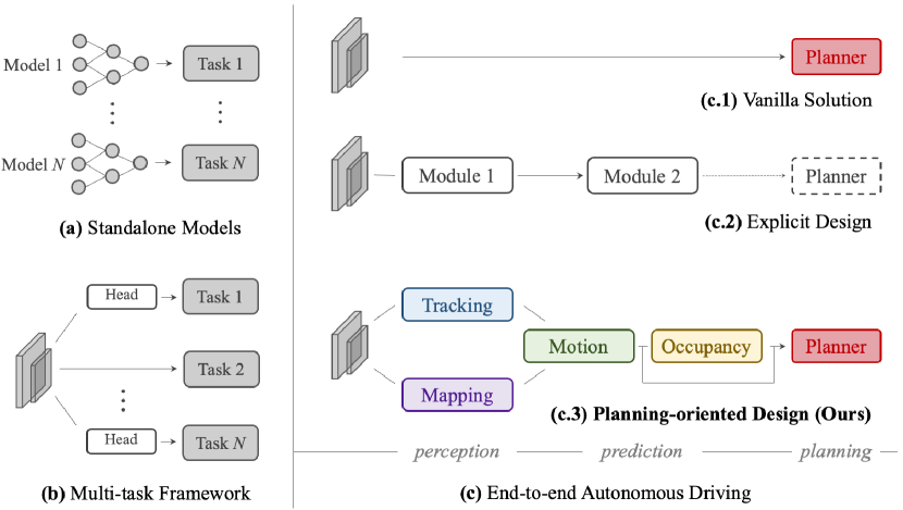
Figure 1: Comparison on the various designs of autonomous driving framework. (a) Most industrial solutions deploy separate models for different tasks. (b) The multi-task learning scheme shares a backbone with divided task heads. (c) The end-to-end paradigm unites modules in perception and prediction. Previous attempts either adopt a direct optimization on planning in (c.1) or devise the system with partial components in (c.2). Instead, we argue in (c.3) that a desirable system should be planning-oriented as well as properly organize preceding tasks to facilitate planning.

A more elegant design is to incorporate a wide span of tasks into a multi-task learning (MTL) paradigm, by plugging several task-specific heads into a shared feature extractor as shown in Fig. 1(b). This is a popular practice in many domains, including general vision [92, 108, 79], autonomous driving [105, 60, 101, 15], such as Transfuser [20], BEVerse [105], and industrialized products, e.g., Mobileye [68], Tesla [87], Nvidia [71], etc. In MTL, the co-training strategy across tasks could leverage feature abstraction; it could effortlessly extend to additional tasks, and save computation cost for onboard chips. However, such a scheme may cause undesirable “negative transfer” [23, 64].

By contrast, the emergence of end-to-end autonomous driving [19, 97, 15, 11, 38] unites all nodes from perception, prediction and planning as a whole. The choice and priority of preceding tasks should be determined in favor of planning. The system should be planning-oriented, exquisitely designed with certain components involved, such that there are few accumulative error as in the standalone option or negative transfer as in the MTL scheme. Table 1 describes the task taxonomy of different framework designs.

Following the end-to-end paradigm, one “tabula-rasa” practice is to directly predict the planned trajectory, without any explicit supervision of perception and prediction as shown in Fig. 1(c.1). Pioneering works [14, 21, 22, 16, 106, 78, 97, 95] verified this vanilla design in the closed-loop simulation [26]. While such a direction deserves further exploration, it is inadequate in safety guarantee and interpretability, especially for highly dynamic urban scenarios. In this paper, we lean toward another perspective and ask the following question: Toward a reliable and planning-oriented autonomous driving system, how to design the pipeline in favor of planning? which preceding tasks are requisite?

Design	Approach	Perception			Prediction		Plan
		Det.	Track	Map	Motion	Occ.
(b)	NMP [101]	✓			✓		✓
	NEAT [19]			✓			✓
	BEVerse [105]	✓		✓		✓
(c.1)	[14, 16, 78, 97]						✓
(c.2)	PnPNet${}^{\text{\textdagger}}$ [57]	✓	✓		✓
	ViP3D${}^{\text{\textdagger}}$ [30]	✓	✓		✓
	P3 [82]					✓	✓
	MP3 [11]			✓		✓	✓
	ST-P3 [38]			✓		✓	✓
	LAV [15]	✓		✓	✓		✓
(c.3)	UniAD (ours)	✓	✓	✓	✓	✓	✓

Table 1: Tasks comparison and taxonomy. “Design” column is classified as in Fig. 1. “Det.” denotes 3D object detection, “Map” stands for online mapping, and “Occ.” is occupancy map prediction. †: these works are not proposed directly for planning, yet they still share the spirit of joint perception and prediction. UniAD conducts five essential driving tasks to facilitate planning.

An intuitive resolution would be to perceive surrounding objects, predict future behaviors and plan a safe maneuver explicitly, as illustrated in Fig. 1(c.2). Contemporary approaches [57, 30, 82, 11, 38] provide good insights and achieve impressive performance. However, we argue that the devil lies in the details; previous works more or less fail to consider certain components (see block (c.2) in Table 1), being reminiscent of the planning-oriented spirit. We elaborate on the detailed definition and terminology, the necessity of these modules in the Supplementary.

To this end, we introduce UniAD, a Unified Autonomous Driving algorithm framework to leverage five essential tasks toward a safe and robust system as depicted in Fig. 1(c.3) and Table 1(c.3). UniAD is designed in a planning-oriented spirit. We argue that this is not a simple stack of tasks with mere engineering effort. A key component is the query-based design to connect all nodes. Compared to the classic bounding box representation, queries benefit from a larger receptive field to soften the compounding error from upstream predictions. Moreover, queries are flexible to model and encode a variety of interactions, e.g., relations among multiple agents. To the best of our knowledge, UniAD is the first work to comprehensively investigate the joint cooperation of such a variety of tasks including perception, prediction and planning in the field of autonomous driving.

The contributions are summarized as follows. (a) we embrace a new outlook of autonomous driving framework following a planning-oriented philosophy, and demonstrate the necessity of effective task coordination, rather than standalone design or simple multi-task learning. (b) we present UniAD, a comprehensive end-to-end system that leverages a wide span of tasks. The key component to hit the ground running is the query design as interfaces connecting all nodes. As such, UniAD enjoys flexible intermediate representations and exchanging multi-task knowledge toward planning. (c) we instantiate UniAD on the challenging benchmark for realistic scenarios. Through extensive ablations, we verify the superiority of our method over previous state-of-the-arts in all aspects.

We hope this work could shed some light on the target-driven design for the autonomous driving system, providing a starting point for coordinating various driving tasks.

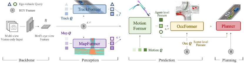
Figure 2: Pipeline of Unified Autonomous Driving (UniAD). It is exquisitely devised following planning-oriented philosophy. Instead of a simple stack of tasks, we investigate the effect of each module in perception and prediction, leveraging the benefits of joint optimization from preceding nodes to final planning in the driving scene. All perception and prediction modules are designed in a transformer decoder structure, with task queries as interfaces connecting each node. A simple attention-based planner is in the end to predict future waypoints of the ego-vehicle considering the knowledge extracted from preceding nodes. The map over occupancy is for visual purpose only.

2 Methodology

Overview.

As illustrated in Fig. 2, UniAD comprises four transformer decoder-based perception and prediction modules and one planner in the end. Queries $Q$ play the role of connecting the pipeline to model different interactions of entities in the driving scenario. Specifically, a sequence of multi-camera images is fed into the feature extractor, and the resulting perspective-view features are transformed into a unified bird’s-eye-view (BEV) feature $B$ by an off-the-shelf BEV encoder in BEVFormer [55]. Note that UniAD is not confined to a specific BEV encoder, and one can utilize other alternatives to extract richer BEV representations with long-term temporal fusion [31, 74] or multi-modality fusion [64, 58]. In TrackFormer, the learnable embeddings that we refer to as track queries inquire about the agents’ information from $B$ to detect and track agents. MapFormer takes map queries as semantic abstractions of road elements (e.g., lanes and dividers) and performs panoptic segmentation of the map. With the above queries representing agents and maps, MotionFormer captures interactions among agents and maps and forecasts per-agent future trajectories. Since the action of each agent can significantly impact others in the scene, this module makes joint predictions for all agents considered. Meanwhile, we devise an ego-vehicle query to explicitly model the ego-vehicle and enable it to interact with other agents in such a scene-centric paradigm. OccFormer employs the BEV feature $B$ as queries, equipped with agent-wise knowledge as keys and values, and predicts multi-step future occupancy with agent identity preserved. Finally, Planner utilizes the expressive ego-vehicle query from MotionFormer to predict the planning result, and keep itself away from occupied regions predicted by OccFormer to avoid collisions.

2.1 Perception: Tracking and Mapping

TrackFormer.

It jointly performs detection and multi-object tracking (MOT) without non-differentiable post-processing. Inspired by [100, 104], we take a similar query design. Besides the conventional detection queries utilized in object detection [8, 109], additional track queries are introduced to track agents across frames. Specifically, at each time step, initialized detection queries are responsible for detecting newborn agents that are perceived for the first time, while track queries keep modeling those agents detected in previous frames. Both detection queries and track queries capture the agent abstractions by attending to BEV feature $B$. As the scene continuously evolves, track queries at the current frame interact with previously recorded ones in a self-attention module to aggregate temporal information, until the corresponding agents disappear completely (untracked in a certain time period). Similar to [8], TrackFormer contains $N$ layers and the final output state $Q_{A}$ provides knowledge of $N_{a}$ valid agents for downstream prediction tasks. Besides queries encoding other agents surrounding the ego-vehicle, we introduce one particular ego-vehicle query in the query set to explicitly model the self-driving vehicle itself, which is further used in planning.

MapFormer.

We design it based on a 2D panoptic segmentation method Panoptic SegFormer [56]. We sparsely represent road elements as map queries to help downstream motion forecasting, with location and structure knowledge encoded. For driving scenarios, we set lanes, dividers and crossings as things, and the drivable area as stuff [50]. MapFormer also has $N$ stacked layers whose output results of each layer are all supervised, while only the updated queries $Q_{M}$ in the last layer are forwarded to MotionFormer for agent-map interaction.

2.2 Prediction: Motion Forecasting

Recent studies have proven the effectiveness of transformer structure on the motion task [63, 99, 43, 44, 69, 84, 70], inspired by which we propose MotionFormer in the end-to-end setting. With highly abstract queries for dynamic agents $Q_{A}$ and static map $Q_{M}$ from TrackFormer and MapFormer respectively, MotionFormer predicts all agents’ multimodal future movements, i.e., top-k possible trajectories, in a scene-centric manner. This paradigm produces multi-agent trajectories in the frame with a single forward pass, which greatly saves the computational cost of aligning the whole scene to each agent’s coordinate [49]. Meanwhile, we pass the ego-vehicle query from TrackFormer through MotionFormer to engage ego-vehicle to interact with other agents, considering the future dynamics. Formally, the output motion is formulated as $\!\{\hat{\mathbf{x}}_{i,k}\!\in\!\mathbb{R}^{T\!\times\!2}|i\!=1,\dots,N_{a};k\!=\!1,\dots,\mathcal{K}\}$ , where $i$ indexes the agent, $k$ indexes the modality of trajectories and $T$ is the length of prediction horizon.

MotionFormer.

It is composed of $N$ layers, and each layer captures three types of interactions: agent-agent, agent-map and agent-goal point. For each motion query $Q_{i,k}$ (defined later, and we omit subscripts $i$, $k$ in the following context for simplicity), its interactions between other agents $Q_{A}$ or map elements $Q_{M}$ could be formulated as:

$$Q_{a/m}=\texttt{MHCA}(\texttt{MHSA}(Q),Q_{A}/Q_{M}),$$ (1)

where MHCA, MHSA denote multi-head cross-attention and multi-head self-attention [91] respectively. As it is also important to focus on the intended position, i.e., goal point, to refine the predicted trajectory, we devise an agent-goal point attention via deformable attention [109] as follows:

$$Q_{g}=\texttt{DeformAttn}(Q,\hat{\mathbf{x}}_{T}^{l-1},B),$$ (2)

where $\hat{\mathbf{x}}_{T}^{l-1}$ is the endpoint of the predicted trajectory of previous layer. $\texttt{DeformAttn}(q,\!r,\!x)$, a deformable attention module, takes in the query $q$, reference point $r$ and spatial feature $x$. It performs sparse attention on the spatial feature around the reference point. Through this, the predicted trajectory is further refined as aware of the endpoint surroundings. All three interactions are modeled in parallel, where the generated $Q_{a}$, $Q_{m}$ and $Q_{g}$ are concatenated and passed to a multi-layer perceptron (MLP), resulting query context $Q_{\text{ctx}}$. Then, $Q_{\text{ctx}}$ is sent to the successive layer for refinement or decoded as prediction results at the last layer.

Motion queries.

The input queries for each layer of MotionFormer, termed motion queries, comprise two components: the query context $Q_{\text{ctx}}$ produced by the preceding layer as described before, and the query position $Q_{\text{pos}}$. Specifically, $Q_{\text{pos}}$ integrates the positional knowledge in four-folds as in Eq. 3: (1) the position of scene-level anchors $I^{s}$; (2) the position of agent-level anchors $I^{a}$; (3) current location of the agent $i$ and (4) the predicted goal point.

$$Q_{\text{pos}}= \text{MLP}(\text{PE}(I^{s}))+\text{MLP}(\text{PE}(I^{a}))$$ (3)

$$+ \text{MLP}(\text{PE}(\hat{\mathbf{x}}_{0}))+\text{MLP}(\text{PE}(\hat{\mathbf{x}}_{T}^{l-1})).$$

Here the sinusoidal position encoding $\text{PE}(\cdot)$ followed by an MLP is utilized to encode the positional points and $\hat{\mathbf{x}}_{T}^{0}$ is set as $I^{s}$ at the first layer (subscripts $i,k$ are also omitted). The scene-level anchor represents prior movement statistics in a global view, while the agent-level anchor captures the possible intention in the local coordinate. They are both clustered by k-means algorithm on the endpoints of ground-truth trajectories, to narrow down the uncertainty of prediction. Contrary to the prior knowledge, the start point provides customized positional embedding for each agent, and the predicted endpoint serves as a dynamic anchor optimized layer-by-layer in a coarse-to-fine fashion.

Non-linear Optimization.

Different from conventional motion forecasting works which have direct access to ground truth perceptual results, i.e., agents’ location and corresponding tracks, we consider the prediction uncertainty from the prior module in our end-to-end paradigm. Brutally regressing the ground-truth waypoints from an imperfect detection position or heading angle may lead to unrealistic trajectory predictions with large curvature and acceleration. To tackle this, we adopt a non-linear smoother [7] to adjust the target trajectories and make them physically feasible given an imprecise starting point predicted by the upstream module. The process is:

$$\tilde{\mathbf{x}}^{*}=\arg\min_{\mathbf{x}}c(\mathbf{x},\tilde{\mathbf{x}}),$$ (4)

where $\tilde{\mathbf{x}}$ and $\tilde{\mathbf{x}}^{*}$ denote the ground-truth and smoothed trajectory, $\mathbf{x}$ is generated by multiple-shooting [3], and the cost function is as follows:

$$c(\mathbf{x},\tilde{\mathbf{x}})=\lambda_{\text{xy}}\lVert\mathbf{x},\tilde{\mathbf{x}}\rVert_{2}+\lambda_{\text{goal}}\lVert\mathbf{x}_{T},\tilde{\mathbf{x}}_{T}\rVert_{2}+\sum_{\phi\in\Phi}\phi(\mathbf{x}),$$ (5)

where $\lambda_{\text{xy}}$ and $\lambda_{\text{goal}}$ are hyperparameters, the kinematic function set $\Phi$ has five terms including jerk, curvature, curvature rate, acceleration and lateral acceleration. The cost function regularizes the target trajectory to obey kinematic constraints. This target trajectory optimization is only conducted in training and does not affect inference.

2.3 Prediction: Occupancy Prediction

Occupancy grid map is a discretized BEV representation where each cell holds a belief indicating whether it is occupied, and the occupancy prediction task is to discover how the grid map changes in the future. Previous approaches utilize RNN structure for temporally expanding future predictions from observed BEV features [35, 38, 105]. However, they rely on highly hand-crafted clustering post-processing to generate per-agent occupancy maps, as they are mostly agent-agnostic by compressing BEV features as a whole into RNN hidden states. Due to the deficient usage of agent-wise knowledge, it is challenging for them to predict the behaviors of all agents globally, which is essential to understand how the scene evolves. To address this, we present OccFormer to incorporate both scene-level and agent-level semantics in two aspects: (1) a dense scene feature acquires agent-level features via an exquisitely designed attention module when unrolling to future horizons; (2) we produce instance-wise occupancy easily by a matrix multiplication between agent-level features and dense scene features without heavy post-processing.

OccFormer is composed of $T_{o}$ sequential blocks where $T_{o}$ indicates the prediction horizon. Note that $T_{o}$ is typically smaller than $T$ in the motion task, due to the high computation cost of densely represented occupancy. Each block takes as input the rich agent features $G^{t}$ and the state (dense feature) $F^{t-1}$ from the previous layer, and generates $F^{t}$ for timestep $t$ considering both instance- and scene-level information. To get agent feature $G^{t}$ with dynamics and spatial priors, we max-pool motion queries from MotionFormer in the modality dimension denoted as $Q_{X}\!\in\!\mathbb{R}^{N_{a}\!\times\!D}$, with $D$ as the feature dimension. Then we fuse it with the upstream track query $Q_{A}$ and current position embedding $P_{A}$ via a temporal-specific MLP:

$$G^{t}=\text{MLP}_{t}([Q_{A},P_{A},Q_{X}]),\ t={1,\dots,T_{o}},$$ (6)

where $[\cdot]$ indicates concatenation. For the scene-level knowledge, the BEV feature $B$ is downscaled to $\nicefrac{{1}}{{4}}$ resolution for training efficiency to serve as the first block input $F^{0}$. To further conserve training memory, each block follows a downsample-upsample manner with an attention module in between to conduct pixel-agent interaction at $\nicefrac{{1}}{{8}}$ downscaled feature, denoted as $F_{\text{ds}}^{t}$.

Pixel-agent interaction

is designed to unify the scene- and agent-level understanding when predicting future occupancy. We take the dense feature $F_{\text{ds}}^{t}$ as queries, instance-level features as keys and values to update the dense feature over time. Detailedly, $F^{t}_{\text{ds}}$ is passed through a self-attention layer to model responses between distant grids, then a cross-attention layer models interactions between agent features ${G^{t}}$ and per-grid features. Moreover, to align the pixel-agent correspondence, we constrain the cross-attention by an attention mask, which restricts each pixel to only look at the agent occupying it at timestep $t$, inspired by [17]. The update process of the dense feature is formulated as:

$$D_{\text{ds}}^{t}=\texttt{MHCA}(\texttt{MHSA}(F_{\text{ds}}^{t}),G^{t},\text{attn\_mask}=O_{m}^{t}).$$ (7)

The attention mask $O_{m}^{t}$ is semantically similar to occupancy, and is generated by multiplying an additional agent-level feature and the dense feature $F_{\text{ds}}^{t}$, where we name the agent-level feature here as mask feature $M^{t}=\text{MLP}({G^{t}})$. After the interaction process in Eq. 7, $D_{\text{ds}}^{t}$ is upsampled to $\nicefrac{{1}}{{4}}$ size of $B$. We further add $D_{\text{ds}}^{t}$ with block input $F^{t-1}$ as a residual connection, and the resulting feature $F^{t}$ is passed to the next block.

Instance-level occupancy.

It represents the occupancy with each agent’s identity preserved. It could be simply drawn via matrix multiplication, as in recent query-based segmentation works [18, 52]. Formally, in order to get an occupancy prediction of original size $H\!\times\!W$ of BEV feature $B$, the scene-level features $F^{t}$ are upsampled to $F_{\text{dec}}^{t}\!\in\!\mathbb{R}^{C\!\times\!H\!\times\!W}$ by a convolutional decoder, where $C$ is the channel dimension. For the agent-level feature, we further update the coarse mask feature $M^{t}$ to the occupancy feature $U^{t}\!\in\!\mathbb{R}^{N_{a}\!\times\!C}$ by another MLP. We empirically find that generating $U^{t}$ from mask feature $M^{t}$ instead of original agent feature ${G^{t}}$ leads to superior performance. The final instance-level occupancy of timestep $t$ is:

$$\hat{O}_{A}^{t}=U^{t}\cdot F_{\text{dec}}^{t}.$$ (8)

2.4 Planning

Planning without high-definition (HD) maps or predefined routes usually requires a high-level command to indicate the direction to go [11, 38]. Following this, we convert the raw navigation signals (i.e., turn left, turn right and keep forward) into three learnable embeddings, named command embeddings. As the ego-vehicle query from MotionFormer already expresses its multimodal intentions, we equip it with command embeddings to form a “plan query”. We attend plan query to BEV features $B$ to make it aware of surroundings, and then decode it to future waypoints $\hat{\tau}$.

To further avoid collisions, we optimize $\hat{\tau}$ based on Newton’s method in inference only by the following:

$$\tau^{*}=\arg\min_{\tau}f(\tau,\hat{\tau},\hat{O}),$$ (9)

where $\hat{\tau}$ is the original planning prediction, $\tau^{*}$ denotes the optimized planning, which is selected from multiple-shooting [3] trajectories $\tau$ as to minimize cost function $f(\cdot)$. $\hat{O}$ is a classical binary occupancy map merged from the instance-wise occupancy prediction from OccFormer. The cost function $f(\cdot)$ is calculated by:

$$f(\tau,\hat{\tau},\hat{O})=\lambda_{\text{coord}}\lVert\tau,\hat{\tau}\rVert_{2}+\lambda_{\text{obs}}\sum_{t}\mathcal{D}(\tau_{t},\hat{O}^{t}),$$ (10)

$$\mathcal{D}(\tau_{t},\hat{O}^{t})=\sum_{(x,y)\in\mathcal{S}}\frac{1}{\sigma\sqrt{2\pi}}\text{exp}(-\frac{\lVert\tau_{t}-(x,y)\rVert_{2}^{2}}{2\sigma^{2}}).$$ (11)

Here $\lambda_{\text{coord}}$, $\lambda_{\text{obs}}$, and $\sigma$ are hyperparameters, and $t$ indexes a timestep of future horizons. The $l_{2}$ cost pulls the trajectory toward the original predicted one, while the collision term $\mathcal{D}$ pushes it away from occupied grids, considering surrounding positions confined to $\mathcal{S}=\{(x,y)|\lVert(x,y)-\tau_{t}\rVert_{2}<d,\hat{O}_{x,y}^{t}=1\}$.

ID	Modules					Tracking			Mapping		Motion Forecasting			Occupancy Prediction				Planning
	Track	Map	Motion	Occ.	Plan	AMOTA$\uparrow$	AMOTP$\downarrow$	IDS$\downarrow$	IoU-lane$\uparrow$	IoU-road$\uparrow$	minADE$\downarrow$	minFDE$\downarrow$	MR$\downarrow$	IoU-n.$\uparrow$	IoU-f.$\uparrow$	VPQ-n.$\uparrow$	VPQ-f.$\uparrow$	avg.L2$\downarrow$	avg.Col.$\downarrow$
0∗	✓	✓	✓	✓	✓	0.356	1.328	893	0.302	0.675	0.858	1.270	0.186	55.9	34.6	47.8	26.4	1.154	0.941
1	✓					0.348	1.333	791	-	-	-	-	-	-	-	-	-	-	-
2		✓				-	-	-	0.305	0.674	-	-	-	-	-	-	-	-	-
3	✓	✓				0.355	1.336	785	0.301	0.671	-	-	-	-	-	-	-	-	-
4			✓			-	-	-	-	-	0.815	1.224	0.182	-	-	-	-	-	-
5	✓		✓			0.360	1.350	919	-	-	0.751	1.109	0.162	-	-	-	-	-	-
6	✓	✓	✓			0.354	1.339	820	0.303	0.672	0.736(-9.7%)	1.066(-12.9%)	0.158	-	-	-	-	-	-
7				✓		-	-	-	-	-	-	-	-	60.5	37.0	52.4	29.8	-	-
8	✓			✓		0.360	1.322	809	-	-	-	-	-	62.1	38.4	52.2	32.1	-	-
9	✓	✓	✓	✓		0.359	1.359	1057	0.304	0.675	0.710(-3.5%)	1.005(-5.8%)	0.146	62.3	39.4	53.1	32.2	-	-
10					✓		-	-	-	-	-	-	-	-	-	-	-	1.131	0.773
11	✓	✓	✓		✓	0.366	1.337	889	0.303	0.672	0.741	1.077	0.157	-	-	-	-	1.014	0.717
12	✓	✓	✓	✓	✓	0.358	1.334	641	0.302	0.672	0.728	1.054	0.154	62.3	39.5	52.8	32.3	1.004	0.430

Table 2: Detailed ablations on the effectiveness of each task. We can conclude that two perception sub-tasks greatly help motion forecasting, and prediction performance also benefits from unifying the two prediction modules. With all prior representations, our goal-planning boosts significantly to ensure safety. UniAD outperforms naive MTL solution by a large margin for prediction and planning tasks, and it also owns the superiority that no substantial perceptual performance drop occurs. Only main metrics are shown for brevity. “avg.L2” and “avg.Col” are the average values across the planning horizon. $\ast$: ID-0 is the MTL scheme with separate heads for each task.

2.5 Learning

UniAD is trained in two stages. We first jointly train perception parts, i.e., the tracking and mapping modules, for a few epochs (6 in our experiments), and then train the model end-to-end for 20 epochs with all perception, prediction and planning modules. The two-stage training is found more stable empirically. We refer the audience to the Supplementary for details of each loss.

Shared matching.

Since UniAD involves instance-wise modeling, pairing predictions to the ground truth set is required in perception and prediction tasks. Similar to DETR [8, 56], the bipartite matching algorithm is adopted in the tracking and online mapping stage. As for tracking, candidates from detection queries are paired with newborn ground truth objects, and predictions from track queries inherit the assignment from previous frames. The matching results in the tracking module are reused in motion and occupancy nodes to consistently model agents from historical tracks to future motions in the end-to-end framework.

3 Experiments

We conduct experiments on the challenging nuScenes dataset [6]. In this section, we validate the effectiveness of our design in three aspects: joint results revealing the advantage of task coordination and its effect on planning, modular results of each task compared with previous methods, and ablations on the design space for specific modules. Due to space limit, the full suite of protocols, some ablations and visualizations are provided in the Supplementary.

3.1 Joint Results

We conduct extensive ablations as shown in Table 2 to prove the effectiveness and necessity of preceding tasks in the end-to-end pipeline. Each row of this table shows the model performance when incorporating task modules listed in the second Modules column. The first row (ID-0) serves as a vanilla multi-task baseline with separate task heads for comparison. The best result of each metric is marked in bold, and the runner-up result is underlined in each column.

Roadmap toward safe planning.

As prediction is closer to planning compared to perception, we first investigate the two types of prediction tasks in our framework, i.e., motion forecasting and occupancy prediction. In Exp.10-12, only when the two tasks are introduced simultaneously (Exp.12), both metrics of the planning L2 and collision rate achieve the best results, compared to naive end-to-end planning without any intermediate tasks (Exp.10, Fig. 1(c.1)). Thus we conclude that both these two prediction tasks are required for a safe planning objective. Taking a step back, in Exp.7-9, we show the cooperative effect of two types of prediction. The performance of both tasks get improved when they are closely integrated (Exp.9, -3.5% minADE, -5.8% minFDE, -1.3 MR(%), +2.4 IoU-f.(%), +2.4 VPQ-f.(%)), which demonstrates the necessity to include both agent and scene representations. Meanwhile, in order to realize a superior motion forecasting performance, we explore how perception modules could contribute in Exp.4-6. Notably, incorporating both tracking and mapping nodes brings remarkable improvement to forecasting results (-9.7% minADE, -12.9% minFDE, -2.3 MR(%)). We also present Exp.1-3, which indicate training perception sub-tasks together leads to comparable results to a single task. Additionally, compared with naive multi-task learning (Exp.0, Fig. 1(b)), Exp.12 outperforms it by a significant margin in all essential metrics (-15.2% minADE, -17.0% minFDE, -3.2 MR(%)), +4.9 IoU-f.(%)., +5.9 VPQ-f.(%), -0.15$m$ avg.L2, -0.51 avg.Col.(%)), showing the superiority of our planning-oriented design.

3.2 Modular Results

Following the sequential order of perception-prediction-planning, we report the performance of each task module in comparison to prior state-of-the-arts on the nuScenes validation set. Note that UniAD jointly performs all these tasks with a single trained network. The main metric for each task is marked with gray background in tables.

Perception results.

As for multi-object tracking in Table 3, UniAD yields a significant improvement of +6.5 and +14.2 AMOTA(%) compared to MUTR3D [104] and ViP3D [30] respectively. Moreover, UniAD achieves the lowest ID switch score, showing its temporal consistency for each tracklet. For online mapping in Table 4, UniAD performs well on segmenting lanes (+7.4 IoU(%) compared to BEVFormer), which is crucial for downstream agent-road interaction in the motion module. As our tracking module follows an end-to-end paradigm, it is still inferior to tracking-by-detection methods with complex associations such as Immortal Tracker [93], and our mapping results trail previous perception-oriented methods on specific classes. We argue that UniAD is to benefit final planning with perceived information rather than optimizing perception with full model capacity.

Prediction results.

Motion forecasting results are shown in Table 5, where UniAD remarkably outperforms previous vision-based end-to-end methods. It reduces prediction errors by 38.3% and 65.4% on minADE compared to PnPNet-vision [57] and ViP3D [30] respectively. In terms of occupancy prediction reported in Table 6, UniAD gets notable advances in nearby areas, yielding +4.0 and +2.0 on IoU-near(%) compared to FIERY [35] and BEVerse [105] with heavy augmentations, respectively.

Planning results.

Benefiting from rich spatial-temporal information in both the ego-vehicle query and occupancy, UniAD reduces planning L2 error and collision rate by 51.2% and 56.3% compared to ST-P3 [38], in terms of the average value for the planning horizon. Moreover, it notably outperforms several LiDAR-based counterparts, which is often deemed challenging for perception tasks.

Method	AMOTA$\uparrow$	AMOTP$\downarrow$	Recall$\uparrow$	IDS$\downarrow$
Immortal Tracker${}^{\text{\textdagger}}$ [93]	0.378	1.119	0.478	936
ViP3D [30]	0.217	1.625	0.363	-
QD3DT [36]	0.242	1.518	0.399	-
MUTR3D [104]	0.294	1.498	0.427	3822
UniAD	0.359	1.320	0.467	906

Table 3: Multi-object tracking. UniAD outperforms previous end-to-end MOT techniques (with image inputs only) on all metrics. †: Tracking-by-detection method with post-association, reimplemented with BEVFormer for a fair comparison.

Method	Lanes$\uparrow$	Drivable$\uparrow$	Divider$\uparrow$	Crossing$\uparrow$
VPN [72]	18.0	76.0	-	-
LSS [76]	18.3	73.9	-	-
BEVFormer [55]	23.9	77.5	-	-
BEVerse${}^{\text{\textdagger}}$ [105]	-	-	30.6	17.2
UniAD	31.3	69.1	25.7	13.8

Table 4: Online mapping. UniAD achieves competitive performance against state-of-the-art perception-oriented methods, with comprehensive road semantics. We report segmentation IoU (%). †: Reimplemented with BEVFormer.

Method	minADE($m$)$\downarrow$	minFDE($m$)$\downarrow$	MR$\downarrow$	EPA$\uparrow$
PnPNet${}^{\text{\textdagger}}$ [57]	1.15	1.95	0.226	0.222
ViP3D [30]	2.05	2.84	0.246	0.226
Constant Pos.	5.80	10.27	0.347	-
Constant Vel.	2.13	4.01	0.318	-
UniAD	0.71	1.02	0.151	0.456

Table 5: Motion forecasting. UniAD remarkably outperforms previous vision-based end-to-end methods. We also report two settings of modeling vehicles with constant positions or velocities as comparisons. †: Reimplemented with BEVFormer.

Method	IoU-n.$\uparrow$	IoU-f.$\uparrow$	VPQ-n.$\uparrow$	VPQ-f.$\uparrow$
FIERY [35]	59.4	36.7	50.2	29.9
StretchBEV [1]	55.5	37.1	46.0	29.0
ST-P3 [38]	-	38.9	-	32.1
BEVerse${}^{\text{\textdagger}}$ [105]	61.4	40.9	54.3	36.1
UniAD	63.4	40.2	54.7	33.5

Table 6: Occupancy prediction. UniAD gets significant improvement in nearby areas, which are more critical for planning. “n.” and “f.” indicates near ($30\!\times\!30m$) and far ($50\!\times\!50m$) evaluation ranges respectively. †: Trained with heavy augmentations.

Method	L2($m$)$\downarrow$				Col. Rate(%)$\downarrow$
	1$s$	2$s$	3$s$	Avg.	1$s$	2$s$	3$s$	Avg.
NMP${}^{\text{\textdagger}}$ [101]	-	-	2.31	-	-	-	1.92	-
SA-NMP${}^{\text{\textdagger}}$ [101]	-	-	2.05	-	-	-	1.59	-
FF${}^{\text{\textdagger}}$ [37]	0.55	1.20	2.54	1.43	0.06	0.17	1.07	0.43
EO${}^{\text{\textdagger}}$ [47]	0.67	1.36	2.78	1.60	0.04	0.09	0.88	0.33
ST-P3 [38]	1.33	2.11	2.90	2.11	0.23	0.62	1.27	0.71
UniAD	0.48	0.96	1.65	1.03	0.05	0.17	0.71	0.31

Table 7: Planning. UniAD achieves the lowest L2 error and collision rate in all time intervals and even outperforms LiDAR-based methods (†) in most cases, verifying the safety of our system.

3.3 Qualitative Results

Fig. 3 visualizes the results of all tasks for one complex scene. The ego vehicle drives with notice to the potential movement of a front vehicle and lane. In the Supplementary, we show more visualizations of challenging scenarios and one promising case for the planning-oriented design, that inaccurate results occur in prior modules while the later tasks could still recover, e.g., the planned trajectory remains reasonable though objects have a large heading angle deviation or fail to be detected in tracking results. Besides, we analyze that failure cases of UniAD are mainly under some long-tail scenarios such as large trucks and trailers, shown in the Supplementary as well.

ID	Scene-l. Anch.	Goal Inter.	Ego $Q$	NLO.	minADE$\downarrow$	minFDE$\downarrow$	MR$\downarrow$	minFDE -mAP∗ $\uparrow$
1					0.844	1.336	0.177	0.246
2	✓				0.768	1.159	0.164	0.267
3	✓	✓			0.755	1.130	0.168	0.264
4	✓	✓	✓		0.747	1.096	0.156	0.266
5	✓	✓	✓	✓	0.710	1.004	0.146	0.273

Table 8: Ablation for designs in the motion forecasting module. All components contribute to the ultimate performance. “Scene-l. Anch.” denotes rotated scene-level anchors. “Goal Inter.” means the agent-goal point interaction. “Ego $Q$” represents the ego-vehicle query and “NLO.” is the non-linear optimization strategy. $\ast$: A metric considering detection and forecasting accuracy simultaneously, and we put details in the Supplementary.

ID	Cross. Attn.	Attn. Mask	Mask Feat.	IoU-n.$\uparrow$	IoU-f.$\uparrow$	VPQ-n.$\uparrow$	VPQ-f.$\uparrow$
1				61.2	39.7	51.5	31.8
2	✓			61.3	39.4	51.0	31.8
3	✓	✓		62.3	39.7	52.4	32.5
4	✓	✓	✓	62.6	39.5	53.2	32.8

Table 9: Ablation for designs in the occupancy prediction module. Cross-attention with masks and the reuse of mask feature helps improve the prediction. “Cross. Attn.” and “Attn. Mask” represent cross-attention and the attention mask in the pixel-agent interaction respectively. “Mask Feat.” denotes the reuse of the mask feature for instance-level occupancy.

ID	BEV	Col.	Occ.	L2$\downarrow$			Col. Rate$\downarrow$
	Att.	Loss	Optim.	1$s$	2$s$	3$s$	1$s$	2$s$	3$s$
1				0.44	0.99	1.71	0.56	0.88	1.64
2	✓			0.44	1.04	1.81	0.35	0.71	1.58
3	✓	✓		0.44	1.02	1.76	0.30	0.51	1.39
4	✓	✓	✓	0.54	1.09	1.81	0.13	0.42	1.05

Table 10: Ablation for designs in the planning module. Results demonstrate the necessity of each preceding task. “BEV Att.” indicates attending to BEV feature. “Col. Loss” denotes collision loss. “Occ. Optim.” is the optimization strategy with occupancy.

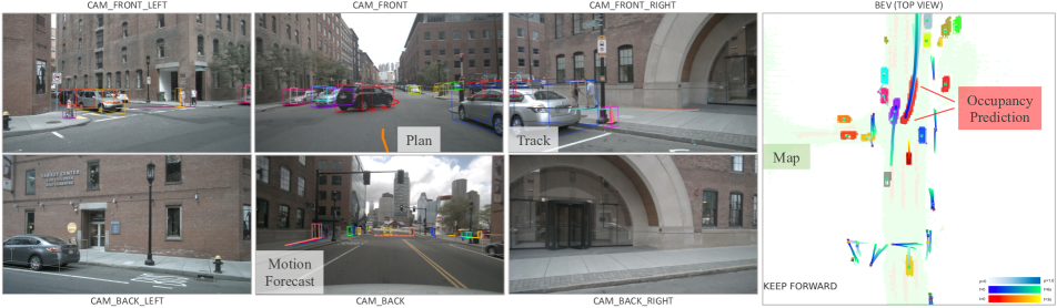
Figure 3: Visualization results. We show results for all tasks in surround-view images and BEV. Predictions from motion and occupancy modules are consistent, and the ego vehicle is yielding to the front black car in this case. Each agent is illustrated with a unique color. Only top-1 and top-3 trajectories from motion forecasting are selected for visualization on image-view and BEV respectively.

3.4 Ablation Study

Effect of designs in MotionFormer.

Table 8 shows that all of our proposed components described in Sec. 2.2 contribute to final performance regarding minADE, minFDE, Miss Rate and minFDE-mAP metrics. Notably, the rotated scene-level anchor shows a significant performance boost (-15.8% minADE, -11.2% minFDE, +1.9 minFDE-mAP(%)), indicating that it is essential to do motion forecasting in the scene-centric manner. The agent-goal point interaction enhances the motion query with the planning-oriented visual feature, and surrounding agents can further benefit from considering the ego vehicle’s intention. Moreover, the non-linear optimization strategy improves the performance (-5.0% minADE, -8.4% minFDE, -1.0 MR(%), +0.7 minFDE-mAP(%)) by taking perceptual uncertainty into account in the end-to-end scenario.

Effect of designs in OccFormer.

As illustrated in Table 9, attending each pixel to all agents without locality constraints (Exp.2) results in slightly worse performance compared to an attention-free baseline (Exp.1). The occupancy-guided attention mask resolves the problem and brings in gain, especially for nearby areas (Exp.3, +1.0 IoU-n.(%), +1.4 VPQ-n.(%)). Additionally, reusing the mask feature $M^{t}$ instead of the agent feature to acquire the occupancy feature further enhances performance.

Effect of designs in Planner.

We provide ablations on the proposed designs in planner in Table 10, i.e., attending BEV features, training with the collision loss and the optimization strategy with occupancy. Similar to previous research [37, 38], a lower collision rate is preferred for safety over naive trajectory mimicking (L2 metric), and is reduced with all parts applied in UniAD.

4 Conclusion and Future Work

We discuss the system-level design for the autonomous driving algorithm framework. A planning-oriented pipeline is proposed toward the ultimate pursuit for planning, namely UniAD. We provide detailed analyses on the necessity of each module within perception and prediction. To unify tasks, a query-based design is proposed to connect all nodes in UniAD, benefiting from richer representations for agent interaction in the environment. Extensive experiments verify the proposed method in all aspects.

Limitations and future work. Coordinating such a comprehensive system with multiple tasks is non-trivial and needs extensive computational power, especially trained with temporal history. How to devise and curate the system for a lightweight deployment deserves future exploration. Moreover, whether or not to incorporate more tasks such as depth estimation, behavior prediction, and how to embed them into the system, are worthy future directions as well.

Acknowledgements. This work is partially supported by National Key R&D Program of China (2022ZD0160100), and in part by Shanghai Committee of Science and Technology (21DZ1100100), and NSFC (62206172).

Appendix

1

Appendix A Task Definition

Detection and tracking.

Detection and tracking are two crucial perception tasks for autonomous driving, and we focus on representing them in the 3D space to facilitate downstream usage. 3D Detection is responsible for locating surrounding objects (coordinates, length, width, height, etc.) at each time stamp; tracking aims at finding the correspondences between different objects across time stamps and associating them temporally (i.e., assigning a consistent track ID for each agent). In the paper, we use multi-object tracking in some cases to denote the detection and tracking process. The final output is a series of associated 3D boxes in each frame, and their corresponding features $Q_{A}$ are forwarded to the motion module. Additionally, note that we have one special query named ego-vehicle query for downstream tasks, which would not be included in the prediction-ground truth matching process and it regresses the location of ego-vehicle accordingly.

Online mapping.

Map intuitively embodies the geometric and semantic information of the environment, and online mapping is to segment meaningful road elements with onboard sensor data (multi-view images in our case) as a substitute for offline annotated high-definition (HD) maps. In UniAD, we model the online map into four categories: lanes, drivable area, dividers and pedestrian crossings, and we segment them in bird’s-eye-view (BEV). Similar to $Q_{A}$, the map queries $Q_{M}$ would be further utilized in the motion forecasting module to model the agent-map interaction.

Motion forecasting.

Bridging perception and planning, prediction plays an important role in the whole autonomous driving system to ensure final safety. Typically, motion forecasting is an independently developed module that predicts agents’ future trajectories with detected bounding boxes and HD maps. And the bounding boxes are ground truth annotations in most current motion datasets [27], which is not realistic in onboard scenarios. While in this paper, the motion forecasting module takes previously encoded sparse queries (i.e., $Q_{A}$ and $Q_{M}$) and dense BEV features $B$ as inputs, and forecasts $\mathcal{K}$ plausible trajectories in future $T$ timesteps for each agent. Besides, to be compatible with our end-to-end and scene-centric scenarios, we predict trajectories as offset according to each agent’s current position. The agent features before the last decoding MLPs, which have encoded both the historical and future information will be sent to the occupancy module for scene-level future understanding. For the ego-vehicle query, it predicts future ego-motion as well (actually providing a coarse planning estimation), and the feature is employed by the planner to generate the ultimate goal.

Occupancy prediction.

Occupancy grid map is a discretized BEV representation where each cell holds a belief indicating whether it is occupied, and the occupancy prediction task is designed to discover how the grid map changes in the future for $T_{o}$ timesteps with multiple agent dynamics. Complementary to motion forecasting which is conditioned on sparse agents, occupancy prediction is densely represented in the whole-scene level. To investigate how the scene evolves with sparse agent knowledge, our proposed occupancy module takes as inputs both the observed BEV feature $B$ and agent features $G^{t}$. After the multi-step agent-scene interaction (detailedly described in Appendix E), the instance-level probability map $\hat{O}_{A}^{t}\!\in\!\mathbb{R}^{N_{a}\!\times\!H\!\times\!W}$ is generated via matrix multiplication between occupancy feature and dense scene feature. To form whole-scene occupancy with agent identity preserved $\hat{O}^{t}\!\in\!\mathbb{R}^{H\!\times\!W}$ which is used for occupancy evaluation and downstream planning, we simply merge the instance-level probability at each timestep using pixel-wise argmax as in [8].

Planning.

As an ultimate goal, the planning module takes all upstream results into consideration. Traditional planning methods in the industry often are rule-based, formulated by “if-else” state machines conditioned on various scenarios which are described with prior detection and prediction results. In our learning-based model, we take the upstream ego-vehicle query, and the dense BEV feature $B$ as input, and predict one trajectory $\hat{\tau}$ for total $T_{p}$ timesteps. Then, the trajectory $\hat{\tau}$ is optimized with the upstream predicted future occupancy $\hat{O}$ to avoid collision and ensure final safety.

Appendix B The Necessity of Each Task

In terms of perception, tracking in the loop as does in PnPNet [57] and ViP3D [30] is proven to complement spatial-temporal features and provide history tracks for occluded agents, refraining from catastrophic decisions for downstream planning. With the aid of HD maps [101, 82, 57, 30] and motion forecasting, planning becomes more accurate toward higher-level intelligence. However, such information is expensive to construct and prone to be outdated, raising the demand for online mapping without HD maps. As for prediction, motion forecasting [10, 42, 41, 29, 107] generates long-term future behaviors and preserves agent identity in form of sparse waypoint outputs. Nonetheless, there exists the challenge to integrate non-differentiable box representation into subsequent planning module [30, 57]. Some recent literature investigates another type of prediction task named occupancy [88] prediction to assist end-to-end planning, in form of cost maps. However, the lack of agent identity and dynamics in occupancy makes it impractical to model social interactions for safe planning. The large computational consumption of modeling multi-step dense features also leads to a much shorter temporal horizon compared to motion forecasting. Therefore, to benefit from the two complementary types of prediction tasks for safe planning, we incorporate both agent-centric motion and whole-scene occupancy in UniAD.

Appendix C Related Work

C.1 Joint perception and prediction

Joint learning of perception and prediction is proposed to avoid the cascading error in traditional modular-independence pipelines. Similar to the motion forecasting task alone, it usually has two types of output representations: agent-level bounding boxes and scene-level occupancy grid maps. Pioneering work FaF [66] predicts boxes in the future and aggregates past information to produce tracklets. IntentNet [10] extends it to reason about intentions and [25, 28] further predict future states in a refinement fashion. Some exploit detection first and utilize agent features in the second prediction stage [9, 53, 75]. Noticing that history information is ignored, PnPNet [57] enriches it by estimating tracking association scores to avert the non-differentiable optimization process as adopted by the tracking-by-detection paradigm [54, 85, 64, 98]. Yet, all these methods rely on non-maximum suppression (NMS) in detection which still leads to information loss. ViP3D [30] which is closely related to our work, employs agent queries in [104] to forecast, taking HD map as another input. We follow the philosophy of [104, 30] in agent track queries, but also develop non-linear optimization on target trajectories to alleviate the potential inaccurate perception problem. Moreover, we introduce an ego-vehicle query for better capturing the ego behaviors in the dynamic environment, and incorporate online mapping to prevent the localization risk or high construction cost with HD map.

The alternative representation, namely the occupancy grid map, discretizes the BEV map into grid cells which holds a belief indicating if it is occupied. Wu et al. [96] estimate a dense motion field, while it could not capture multimodal behaviors. Fishing Net [33] also predicts deterministic future BEV semantic segmentation with multiple sensors. To address this, P3 [82] proposes non-parametric distribution of future semantic occupancy and FIERY [35] devises the first paradigm for multi-view cameras. A few methods improve the performance of FIERY with more sophisticated uncertainty modeling [38, 1, 105]. Notably, this representation could easily extend to motion planning for collision avoidance [82, 11, 38], while it loses the agent identity characteristic and takes a heavy burden to computation which may constrain the prediction horizon. In contrast, we leverage agent-level information for occupancy prediction and ensure accurate and safe planning by unifying these two modes.

C.2 Joint prediction and planning

PRECOG [81] proposes a recurrent model that conditions forecasting on the goal position of the ego vehicle, while PiP [86] generates agents’ motion considering complete presumed planning trajectories. However, producing a rough future trajectory is still challenging in the real world, toward which [62] presents a deep structured model to derive both prediction and planning from the same set of learnable costs. [40, 39] couple the prediction model with classic optimization methods. Meanwhile, some motion forecasting methods implicitly include the planning task by producing their future trajectories simultaneously [12, 70, 45]. Similarly, we encode possible behaviors of the ego vehicle in the scene-centric motion forecasting module, but the interpretable occupancy map is utilized to further optimize the plan to stay safe.

C.3 End-to-end motion planning

End-to-end motion planning has been an active research domain since Pomerleau [77] uses a single neural network that directly predicts control signals. Subsequent studies make great advances especially in closed-loop simulation with deeper networks [4], multi-modal inputs [2, 21, 78], multi-task learning [97, 20], reinforcement learning [59, 46, 89, 13, 14] and distillation from certain privilege knowledge [16, 106, 103]. However, for such methods of directly generating control outputs from sensor data, the transfer from the synthetic environment to realistic application remains a problem considering their robustness and safety assurance [22, 38]. Thus researchers aim at explicitly designing the intermediate representations of the network to prompt safety, where predicting how the scene evolves attracts broad interest. Some works [19, 83, 34] jointly decode planning and BEV semantic predictions to enhance interpretability, while PLOP [5] adopts a polynomial formulation to provide smooth planning results for both ego vehicle and neighbors. Cui et al. [24] introduce a contingency planner with diverse sets of future predictions and LAV [15] trains the planner with all vehicles’ trajectories to provide richer training data. NMP [101] and its variant [94] estimate a cost volume to select the plan with minimal cost besides deterministic future perception. Though they risk producing inconsistent results between two modules, the cost map design is intuitive to recover the final plan in complex scenarios. Inspired by [101], most recent works [102, 82, 11, 38, 37] propose models that construct costs with both learned occupancy prediction and hand-crafted penalties. However, their performances heavily rely on the tailored cost based on human experience and the distribution from where trajectories are sampled [47]. Contrary to these approaches, we leverage the ego-motion information without sophisticated cost design and present the first attempt that incorporates the tracking module along with two genres of prediction representations simultaneously in an end-to-end model.

Appendix D Notations

We provide a lookup table of notations and their shapes mentioned in this paper in Table 11 for reference.

Notation	Shape & Params.	Description
$Q_{o}$	900	number of initial object queries
$D$	256	embed dimensions
$B$	$200\times 200\times 256$	BEV feature encoded by a multi-view framework
$N$	6	number of transformer decoder layers for TrackFormer
$N$	6	number of transformer decoder layers for MapFormer
$N$	4	number of mask decoder layers for MapFormer
$N$	3	number of transformer decoder layers for MotionFormer
$N$	5	number of transformer decoder layers for OccFormer
$N$	3	number of transformer decoder layers for Planner
$N_{a}$	dynamic	number of agents from TrackFormer
$N_{m}$	300	number of map queries from MapFormer
$Q_{A}$	$N_{a}\times 256$	agent features from TrackFormer
$P_{A}$	$N_{a}\times 256$	agent positions from TrackFormer
$Q_{M}$	$N_{m}\times 256$	map features from MapFormer
$\mathcal{K}$	6	number of forecasting modality in MotionFormer
$\tilde{\mathbf{x}}$	$T\times 2$	ground truth for one agent’s motion forecasting
$\hat{\mathbf{x}}$	$N_{a}\times T\times 2$	prediction of motion forecasting
$T$	12	length of prediction timestamps in MotionFormer
$Q_{\text{pos}}$	$N_{a}\times\mathcal{K}\times 256$	query position in MotionFormer
$Q_{\text{ctx}}$	$N_{a}\times\mathcal{K}\times 256$	query context in MotionFormer
$Q_{a}$	$N_{a}\times\mathcal{K}\times 256$	motion query after agent-agent interaction in MotionFormer
$Q_{m}$	$N_{a}\times\mathcal{K}\times 256$	motion query after agent-map interaction in MotionFormer
$Q_{g}$	$N_{a}\times\mathcal{K}\times 256$	motion query after agent-goal point interaction in MotionFormer
$l$	-	index of decoder layer
$PE$	-	sinusoidal position encoding function
$I^{s}$	$\mathcal{K}\times T\times 2$	scene-level anchor position in MotionFormer
$I^{a}$	$\mathcal{K}\times T\times 2$	agent-level anchor position in MotionFormer
$\Phi$	-	kinematic cost function set
$T_{o}$	5	length of prediction timestamps in OccFormer
$G^{t}$	$N_{a}\times 256$	agent feature input
$F^{t}$	$200\times 200\times 256$	future state output
$Q_{X}$	$N_{a}\times 256$	motion query (max-pooled on modality level) from the last layer of MotionFormer
$F_{\text{ds}}^{t}$	$25\times 25\times 256$	downscaled dense feature
$F_{\text{dec}}^{t}$	$200\times 200\times 256$	decoded dense feature after convolutional decoder
$D_{\text{ds}}^{t}$	$25\times 25\times 256$	agent-aware dense feature after pixel-agent interaction
$\hat{O}_{A}^{t}$	$N_{a}\times 200\times 200$	instance-level probability map
$\hat{O}^{t}$	$200\times 200$	classical instance-agnostic occupancy map merged from $\hat{O}_{A}^{t}$ for planning
$O_{m}^{t}$	$200\times 200$	attention mask for pixel-agent interaction
$M^{t}$	$N_{a}\times 256$	mask feature
$U^{t}$	$N_{a}\times 256$	occupancy feature
$T_{p}$	6	length of planning timestamps in Planner
$\hat{\tau}$	$T_{p}\times 2$	planned trajectory before the optimization with occupancy prediction
$\tau^{*}$	$T_{p}\times 2$	ultimate plan output
$\lambda$	-	hyperparameters in cost functions, target functions, etc.

Table 11: Lookup table of notations and hyperparameters in the paper. The superscript $t$ in certain notations denotes the $t^{th}$ block of OccFormer, and is omitted in descriptions for simplicity.

Appendix E Implementation Details

E.1 Detection and Tracking

We inherit most of the detection designs from BEVFormer [55] which takes a BEV encoder to transform image features into BEV feature $B$ and adopts a Deformable DETR head [109] to perform detection on $B$. To further conduct end-to-end tracking without heavy post association, we introduce another group of queries named track queries as in MOTR [100] which continuously tracks previously observed instances according to its assigned track ID. We introduce the tracking process in detail below.

Training stage: At the beginning (i.e., first frame) of each training sequence, all queries are considered detection queries and predict all newborn objects, which is actually the same as BEVFormer. Detection queries are matched to the ground truth by the Hungarian algorithm [8]. They will be stored and updated via the query interaction module (QIM) for the next timestamp serving as track queries following MOTR [100]. In the next timestamp, track queries will be directly matched with a part of ground-truth objects according to the corresponding track ID, and detection queries will be matched with the remaining ground-truth objects (newborn objects). To stabilize training, we adopt the 3D IoU metric to filter the matched queries. Only those predictions having the 3D IoU with ground-truth boxes larger than a certain threshold (0.5 in practice) will be stored and updated.

Inference stage: Different from the training stage, each frame of a sequence is sent to the network sequentially, meaning that track queries could exist for a longer horizon than the training time. Another difference emerging in the inference stage is about query updating, that we use classification scores to filter the queries (0.4 for detection queries and 0.35 for track queries in practice) instead of the 3D IoU metric since the ground truth is not available. Besides, to avoid the interruption of tracklets caused by short-time occlusion, we use a lifecycle mechanism for the tracklets in the inference stage. Specifically, for each track query, it will be considered to disappear completely and be removed only when its corresponding classification score is smaller than 0.35 for a continuous period (2$s$ in practice).

E.2 Online Mapping

Following [56], we decompose the map query set into thing queries and stuff queries. The thing queries model instance-wise map elements (i.e., lanes, boundaries, and pedestrian crossings) and are matched with ground truth via bipartite matching, while the stuff query is only in charge of semantic elements (i.e., drivable area) and is processed with a class-fixed assignment. We set the total number of thing queries to 300 and only 1 stuff query for the drivable area. Also, we stack 6 location decoder layers and 4 mask decoder layers (we follow the structure of those layers as in [56]). We empirically choose thing queries after the location decoder as our map queries $Q_{M}$ for downstream tasks.

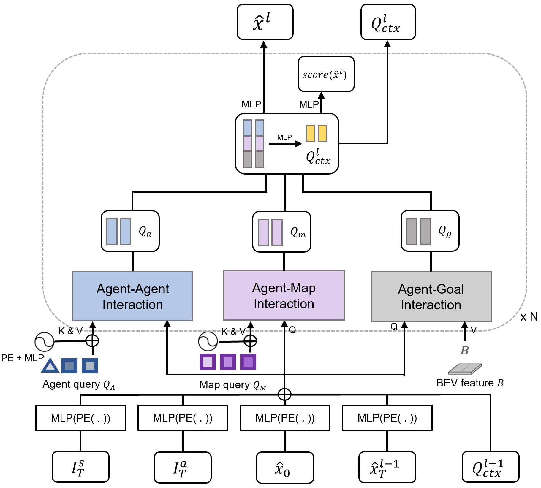
Figure 4: MotionFormer. It consists of $N$ stacked agent-agent, agent-map, and agent-goal interaction transformers. The agent-agent, and agent-map interaction modules are built with standard transformer decoder layers. The agent-goal interaction module is constructed upon the deformable cross-attention module [109]. $I^{s}_{T}$: the end point of scene-level anchor, $I^{a}_{T}$: the end point of clustered agent-level anchor, $\hat{x}_{0}$: the agent’s current position, $\hat{x}_{T}^{l-1}$: the predicted goal point from the previous layer, $Q_{\text{ctx}}^{l-1}$: query context from the previous layer.

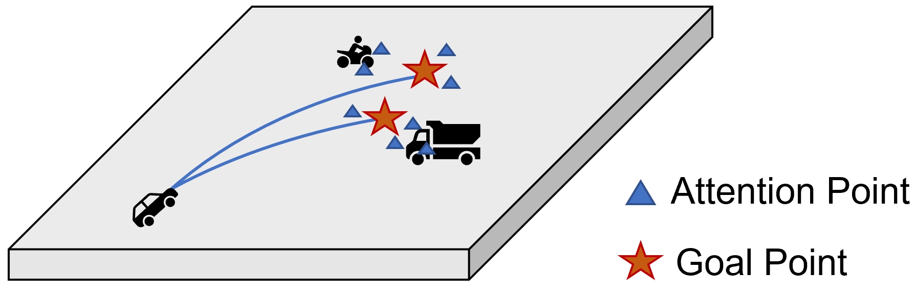
Figure 5: Illustration of agent-goal interaction Module. The BEV visual feature is sampled near each agent’s goal points with deformable cross-attention.

E.3 Motion Forecasting

To better illustrate the details, we provide a diagram as shown in Fig. 4. Our MotionFormer takes $I^{a}_{T}$, $I^{s}_{T}$, $\hat{x}_{0}$, $\hat{x}_{T}^{l-1}\in\mathbb{R}^{\mathcal{K}\times 2}$ to embed query position, and takes $Q_{ctx}^{l-1}$ as query context. Specifically, the anchors are clustered among training data of all agents by the k-means algorithm, and we set $\mathcal{K}\!=\!6$ which is compatible with our output modalities. To embed the scene-level prior, the anchor $I^{a}_{T}$ is rotated and translated into the global coordinate frame according to each agent’s current location and heading angle, which is denoted as $I^{s}_{T}$, as shown in Eq. 12,

$$I_{i,T}^{s}=R_{i}I_{T}^{a}+T_{i},$$ (12)

where $i$ is the index of the agent, and it is omitted later for brevity. To facilitate the coarse-to-fine paradigm, we also adopt the goal point predicted from the previous layer $\hat{x}_{T}^{l-1}$. In the meantime, the agent’s current position is broadcast across the modality, denoted as $\hat{x}_{0}$. Then, MLPs and sinusoidal positional embeddings are applied for each of the prior positional knowledge and we summarize them as the query position $Q_{\text{pos}}\in\mathbb{R}^{\mathcal{K}\times\mathcal{D}}$, which is of the same shape as the query context $Q_{ctx}$. $Q_{\text{pos}}$ and $Q_{\text{ctx}}$ together build up our motion query. We set $\mathcal{D}$ to 256 throughout MotionFormer.

As shown in Fig. 4, our MotionFormer consists of three major transformer blocks, i.e., agent-agent, agent-map and agent-goal interaction modules. The agent-agent, agent-map interaction modules are built with standard transformer decoder layers, which are composed of a multi-head self-attention (MHSA) layer and a multi-head cross-attention (MHCA) layer, a feed-forward network (FFN) and several residual and normalization layers in between [8]. Apart from the agent queries $Q_{A}$ and map queries $Q_{M}$, we also add the positional embeddings to those queries with sinusoidal positional embedding followed by MLP layers. The agent-goal interaction module is built upon deformable cross-attention module [109], where the goal point from the previously predicted trajectory ($R_{i}\hat{x}_{i,T}^{l-1}+T_{i}$) is adopted as the reference point, as shown in Fig. 5. Specifically, we set the number of sampled points to 4 per trajectory, and 6 trajectories per agent as we mention above. The output features of each interaction module are concatenated and projected with MLP layers to dimension $\mathcal{D}\!=\!256$. Then, we use Gaussian Mixture Model to build each agent’s trajectories, where $\hat{x}_{l}\in\mathcal{R}^{\mathcal{K}\times T\times 5}$. We set the prediction time horizon $T$ to 12 (6 seconds) in UniAD. Note that we only take the first two of the last dimension (i.e., $x$ and $y$) as final output trajectories. Besides, the scores of each modality are also predicted ($score(\hat{x}_{l})\in\mathcal{R}^{\mathcal{K}}$). We stack the overall modules for $N$ times, and $N$ is set to 3 in practice.

E.4 Occupancy Prediction

Given the BEV feature from upstream modules, we first downsample it by /4 with convolutional layers for efficient multi-step prediction, then pass it to our proposed OccFormer. OccFormer is composed of $T_{o}$ sequential blocks shown in Fig. 6, where $T_{o}\!=\!5$ is the temporal horizon (including current and future frames) and each block is responsible for generating occupancy of one specific frame. Different from prior works which are short of agent-level knowledge, our proposed method incorporates both dense scene features and sparse agent features when unrolling the future representations. The dense scene feature is from the output of the last block (or the observed feature for current frame) and it’s further downscaled (/8) by a convolution layer to reduce computation for pixel-agent interaction. The sparse agent feature is derived from the concatenation of track query $Q_{A}$, agent positions $P_{A}$, and motion query $Q_{X}$, and it is then passed to a temporal-specific MLP for temporal sensitivity. We conduct pixel-level self-attention to model the long-term dependency required in some rapidly changing scenes, then perform scene-agent incorporation by attending each pixel of the scene to corresponding agents. To enhance the location alignment between agents and pixels, we restrict the cross-attention with an attention mask which is generated by a matrix multiplication between mask feature and downscaled scene feature, where the mask feature is produced by encoding agent feature with an MLP. We then upsample the attended dense feature to the same resolution as input $F^{t-1}$ (/4) and add it with $F^{t-1}$ as a residual connection for stability. The resulting feature $F^{t}$ is both sent to the next block and a convolutional decoder for predicting occupancy at the original BEV resolution (/1). We reuse the mask feature and pass it to another MLP to form occupancy feature, and the instance-level occupancy is therefore generated by a matrix multiplication between occupancy feature and decoded dense feature $F^{t}_{\text{dec}}$ (/1). Note that the MLP layer for mask feature, the MLP layer for occupancy feature, and the convolutional decoder are shared across all $T_{o}$ blocks while other components are independent in each block. Dimensions of all dense features and agent features are 256 in OccFormer.

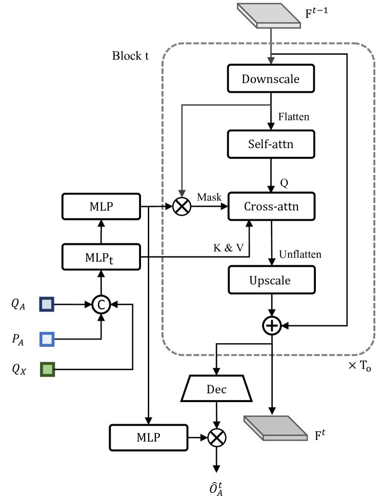
Figure 6: OccFormer. It is composed of $T_{o}$ sequential blocks where $T_{o}$ is the temporal horizon (including current and future frames) and each block is responsible for generating occupancy of one specific frame. We incorporate both dense scene features and sparse agent features, which are encoded from upstream track query $Q_{A}$, agent position $P_{A}$ and motion query $Q_{X}$, to inject agent-level knowledge into future scene representations. We form instance-level occupancy $\hat{O}_{A}^{t}$ via a matrix multiplication between agent-level feature and decoded dense feature at the end of each block.

E.5 Planning

As shown in Fig. 7, our planner takes the ego-vehicle query generated from the tracking and motion forecasting module, which is symbolized with the blue triangle and yellow rectangle respectively. These two queries, along with the command embedding, are encoded with MLP layers followed by a max-pooling layer across the modality dimension, where the most salient modal features are selected and aggregated. The BEV feature interaction module is built with standard transformer decoder layers, and it is stacked for $N$ layers, where we set $N\!=\!3$ here. Specifically, it cross-attends the dense BEV feature with the aggregated plan query. More qualitative results can be found in Sec. F.5 showing the effectiveness of this module. To embed location information, we fuse the plan-query with learned position embedding and the BEV feature with sinusoidal positional embedding. We then regress the planning trajectory with MLP layers, which is denoted as $\hat{\tau}\in\mathcal{R}^{T_{p}\times 2}$. Here we set $T_{p}\!=\!6$ (3 seconds). Finally, we devise the collision optimizer for obstacle avoidance, which takes the predicted occupancy $\hat{O}$ and trajectory $\hat{\tau}$ as input as Eq. 10 in the main paper. We set $d\!=\!5$, $\sigma\!=\!1.0$, $\lambda_{\text{coord}}\!=\!1.0$, $\lambda_{\text{obs}}\!=\!5.0$.

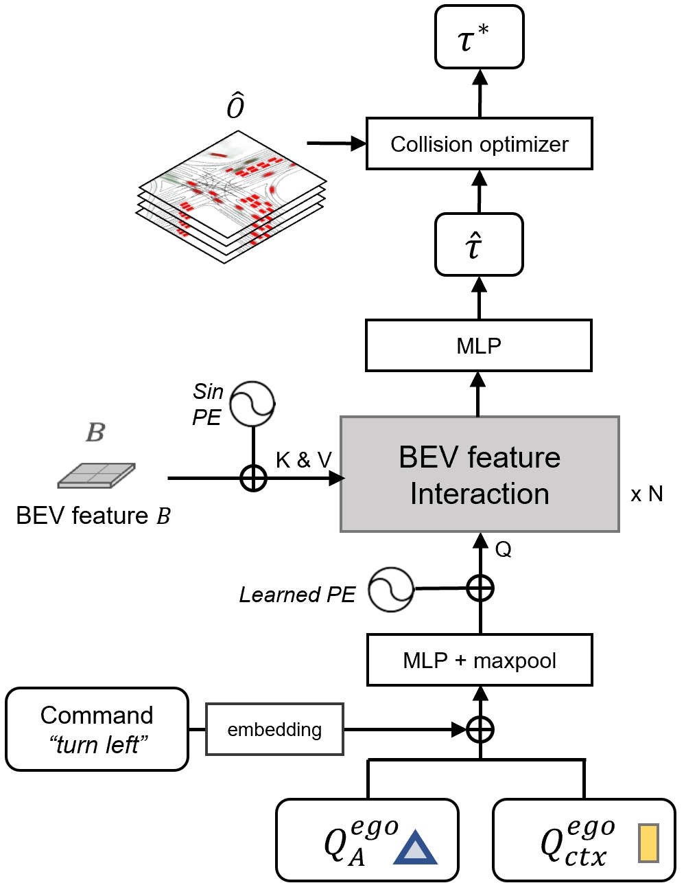
Figure 7: Planner. $Q_{A}^{\text{ego}}$ and $Q_{\text{ctx}}^{\text{ego}}$ are the ego-vehicle query from the tracking and motion forecasting modules, respectively. Along with the high-level command, they are encoded with MLP layers followed by a max-pooling layer across the modality dimension, where the most salient modal features are selected and aggregated. The BEV feature interaction module is built with standard transformer decoder layers, and it is stacked for $N$ layers.

E.6 Training Details

Joint learning.

UniAD is trained in two stages which we find more stable. In stage one, we pre-train perception tasks including tracking and online mapping to stabilize perception predictions. Specifically, we load corresponding pre-trained BEVFormer [55] weights to UniAD for fast convergence including image backbone, FPN, BEV encoder and detection decoder except for object query embeddings (due to the additional ego-vehicle query). We stop the gradient back-propagation in the image backbone to reduce memory cost and train UniAD for 6 epochs with tracking and online mapping losses as follows:

$$L_{1}=L_{\text{track}}+L_{\text{map}}.$$ (13)

In stage two, we keep the image backbone frozen as well, and additionally freeze BEV encoder, which is used for view transformation from image view to BEV, to further reduce memory consumption with more downstream modules. UniAD now is trained with all task losses including tracking, mapping, motion forecasting, occupancy prediction, and planning for 20 epochs (for various ablation studies in main paper, it’s trained for 8 epochs for efficiency):

$$L_{2}=L_{\text{track}}+L_{\text{map}}+L_{\text{motion}}+L_{\text{occ}}+L_{\text{plan}}.$$ (14)

Detailed losses and hyperparameters within each term of $L_{1}$ and $L_{2}$ are described below individually. The length of each training sequence (at each step) for tracking and BEV feature aggregation[55] in both stages is 5 (3 in ablation studies for efficiency).

Detection&tracking loss.

Following BEVFormer [55], the Hungarian loss is adopted for each paired result, which is a linear combination of a Focal loss [61] for class labels and an $l_{1}$ for 3D boxes localization. In terms of the matching strategy, candidates from newborn queries are paired with ground truth objects through bipartite matching, and predictions from track queries inherit the assigned ground truth index from previous frames. Specifically, $L_{\text{track}}=\lambda_{\text{focal}}L_{\text{focal}}+\lambda_{l_{1}}L_{l_{1}}$, where $\lambda_{\text{focal}}\!=\!2$ and $\lambda_{l_{1}}\!=\!0.25$.

Online mapping loss.

As in [56], this includes thing losses for lanes, dividers, and contours, also a stuff loss for the drivable area, where Focal loss is responsible for classification, L1 loss is responsible for thing bounding boxes, Dice loss and GIoU loss[80] account for segmentation. Detailedly, $L_{\text{map}}=\lambda_{\text{focal}}L_{\text{focal}}+\lambda_{l_{1}}L_{l_{1}}+\lambda_{\text{giou}}L_{\text{giou}}+\lambda_{\text{dice}}L_{\text{dice}}$, with $\lambda_{\text{focal}}\!=\!\lambda_{\text{giou}}\!=\!\lambda_{\text{dice}}\!=\!2$ and $\lambda_{l_{1}}\!=\!0.25$.

Motion forecasting loss.

Like most of the prior methods, we model the multimodal trajectories as gaussian mixtures, and use the multi-path loss [12, 90], which includes a classification score loss $L_{\text{cls}}$ and a negative log-likelihood loss term $L_{\text{nll}}$, and $\lambda$ denotes the corresponding weight: $L_{\text{motion}}=\lambda_{\text{cls}}L_{\text{cls}}+\lambda_{\text{reg}}L_{\text{nll}}$, where $\lambda_{\text{cls}}\!\!=\!\!\lambda_{\text{reg}}\!\!=\!\!0.5$. To ensure the temporal smoothness of trajectories, we predict agents’ speed at each timestep first and accumulate it across time to obtain their final trajectories [41].

Occupancy prediction loss.

The output of instance-level occupancy prediction is a binary segmentation of each agent, therefore we adopt binary cross-entropy and Dice loss [67] as the occupancy loss. Formally, $L_{\text{occ}}=\lambda_{\text{bce}}L_{\text{bce}}+\lambda_{\text{dice}}L_{\text{dice}}$, with $\lambda_{\text{bce}}\!=\!5$ and $\lambda_{\text{dice}}\!=\!1$ here. Additionally, since the attention mask in the pixel-agent interaction module could be seen as a coarse prediction, we employ an auxiliary occupancy loss with the same form to supervise it.

Planning loss.

Safety is the most crucial factor in planning. Therefore, apart from the naive imitation $l_{2}$ loss, we employ another collision loss which keeps the planned trajectory away from obstacles as follows:

$$L_{\text{col}}(\hat{\tau},\delta)=\sum_{i,t}\texttt{IoU}(box(\hat{\tau}_{t},w+\delta,l+\delta),b_{i,t})),$$ (15)

$$L_{\text{plan}}=\lambda_{\text{imi}}|\hat{\tau},\tilde{\tau}|_{2}+\lambda_{\text{col}}\sum_{(\omega,\delta)}\omega L_{\text{col}}(\hat{\tau},\delta),$$ (16)

where $\lambda_{\text{imi}}\!=\!1$, $\lambda_{\text{col}}\!=\!2.5$, $(\omega,\delta)$ is a weight-value pair considering additional safety distance, $box(\hat{\tau}_{t},w\!+\!\delta,l\!+\!\delta)$ represents the ego bounding box with an increased size at timestamp $t$ to keep a larger safe distance, and $b_{i,t}$ indicates each agent forecasted in the scene. In practice, we set $(\omega,\delta)$ to $(1.0,0.0),(0.4,0.5),(0.1,1.0)$.

Appendix F Experiments

F.1 Protocols

We follow most of the basic training settings as in BEVFormer [55] for both two stages with a batch size of 1, a learning rate of $2\!\times\!10^{-4}$, learning rate multiplier of the backbone 0.1 and AdamW optimizer [65] with a weight decay of $1\!\times\!10^{-2}$. The default size of BEV size is $200\!\times\!200$, covering BEV ranges of [-51.2$m$, 51.2$m$] for both X and Y axis with the interval as 0.512$m$. More hyperparameters related to feature dimensions are shown in Table 11. Experiments are conducted with 16 NVIDIA Tesla A100 GPUs.

F.2 Metrics

Multi-object tracking.

Following the standard evaluation protocols, we use AMOTA (Average Multi-object Tracking Accuracy), AMOTP (Average Multi-object Tracking Precision), Recall, and IDS (Identity Switches) to evaluate the 3D tracking performance of UniAD on nuScenes dataset. AMOTA and AMOTP are computed by integrating MOTA (Multi-object Tracking Accuracy) and MOTP (Multi-object Tracking Precision) values over all recalls:

$$\text{AMOTA}=\frac{1}{n-1}\sum_{r\in\{\frac{1}{n-1},\frac{2}{n-1},...,1\}}\text{MOTA}_{r},$$ (17)

$$\text{MOTA}_{r}=\mathop{\max}(0,1-\frac{\text{FP}_{r}+\text{FN}_{r}+\text{IDS}_{r}-(1-r)\text{GT}}{r\text{GT}}),$$ (18)

where $\text{FP}_{r}$, $\text{FN}_{r}$, and $\text{IDS}_{r}$ represent the number of false positives, false negatives and identity switches computed at the corresponding recall $r$, respectively. GT stands for the number of ground truth objects in this frame. AMOTP can be defined as:

$$\text{AMOTP}=\frac{1}{n-1}\sum_{r\in\{\frac{1}{n-1},\frac{2}{n-1},...,1\}}\frac{\sum_{i,t}d_{i,t}}{\text{TP}_{r}},$$ (19)

where $d_{i,t}$ denotes the position error (in $x$ and $y$ axis) of matched track $i$ at time stamp $t$, and $\text{TP}_{r}$ is the number of true positives at the corresponding recall $r$.

Online mapping.

We have four categories for the online mapping task, i.e., lanes, boundaries, pedestrian crossings and drivable area. We calculate the intersection-over-union (IoU) metric for each class between the network outputs and ground truth maps.

Motion forecasting.

On one hand, following the standard motion prediction protocols, we adopt conventional metrics, including minADE (minimum Average Displacement Error), minFDE (minimum Final Displacement Error) and MR (Miss Rate). Similar to the prior works [66, 57, 75], these metrics are only calculated within matched TPs, and we set the matching threshold to 1.0$m$ in all of our experiments. As for the MR, we set the miss FDE threshold to 2.0$m$. On the other hand, we also employ recently proposed end-to-end metrics, i.e., EPA (End-to-end Prediction Accuracy) [30] and minFDE-AP [75]. For EPA, we use the same setting as in ViP3D [30] for a fair comparison. For minFDE-AP, we do not separate ground truth into multiple bins (static, linear, and non-linearly moving sub-categories) for simplicity. Specifically, only when an object’s perception location and its min-FDE are within the distance threshold (1.0$m$ and 2.0$m$ respectively), it would be counted as a TP for the AP (average precision) calculation. Similarly to the prior works, we merge the car, truck, construction vehicle, bus, trailer, motorcycle, and bicycle as the vehicle category, and all the motion forecasting metrics provided in the experiments are evaluated on the vehicle category.

Methods	Encoder	Tracking			Mapping		Motion Forecasting				Occupancy Prediction				Planning
		AMOTA$\uparrow$	AMOTP$\downarrow$	IDS$\downarrow$	IoU-lane$\uparrow$	IoU-road$\uparrow$	minADE$\downarrow$	minFDE$\downarrow$	MR$\downarrow$	EPA$\uparrow$	IoU-n.$\uparrow$	IoU-f.$\uparrow$	VPQ-n.$\uparrow$	VPQ-f.$\uparrow$	avg.L2$\downarrow$	avg.Col.$\downarrow$
UniAD-S	R50	0.241	1.488	958	0.315	0.689	0.788	1.126	0.156	0.381	59.4	35.6	49.2	28.9	1.04	0.32
UniAD-B	R101	0.359	1.320	906	0.313	0.691	0.708	1.025	0.151	0.456	63.4	40.2	54.7	33.5	1.03	0.31
UniAD-L	V2-99∗	0.409	1.259	1583	0.323	0.709	0.723	1.067	0.158	0.508	64.1	42.6	55.8	36.9	1.03	0.29

Table 12: Comparisons between three variations of UniAD. $\ast$: pre-trained with extra depth data [73].

Occupancy prediction.

We evaluate the quality of predicted occupancy in both whole-scene level and instance-level following [35, 105]. Specifically, The IoU measures the whole-scene categorical segmentations which is instance-agnostic, while the Video Panoptic Quality (VPQ) [48] takes into account each instance’s presence and consistency over time. The VPQ metric is calculated as follows:

$$\text{VPQ}=\sum_{t=0}^{H}\frac{\sum_{(p_{t},q_{t})\in\text{TP}_{t}}\texttt{IoU}(p_{t},q_{t})}{|\text{TP}_{t}|+\frac{1}{2}|\text{FP}_{t}|+\frac{1}{2}|\text{FN}_{t}|},$$ (20)

where $H$ is the future horizon and we set $H\!=\!4$ (which leads to $T_{o}\!=\!5$ including the current timestamp) as in [35, 105], covering 2.0$s$ consecutive data at 2Hz. $\text{TP}_{t}$, $\text{FP}_{t}$, and $\text{FN}_{t}$ are the set of true positives, false positives, and false negatives at timestamp $t$ respectively. Both two metrics are evaluated under two different BEV ranges, near (“-n.”) for $30m\!\times\!30m$ and far (“-f.”) for $100m\!\times\!100m$ around the ego vehicle. We evaluate the results of the current step ($t\!=\!0$) and the future 4 steps together on both metrics.

ID	Det.	Track	Map	Motion	Occ.	Plan	#Params	FLOPs	FPS
0[105]	✓		✓		✓		102.5M	1921G	-
1	✓						65.9M	1324G	4.2
2	✓	✓					68.2M	1326G	2.7
3	✓	✓	✓				95.8M	1520G	2.2
4	✓	✓	✓	✓			108.6M	1535G	2.1
5	✓	✓	✓	✓	✓		122.5M	1701G	2.0
6	✓	✓	✓	✓	✓	✓	125.0M	1709G	1.8

Table 13: Computational complexity and runtime with different modules incorporated. ID.1 is similar to original BEVFormer [55], and ID. 0 (BEVerse-Tiny) [105] is an MTL framework.

Planning.

We adopt the same metrics as in ST-P3 [38], i.e., L2 error and collision rate at various timestamps.

F.3 Model complexity and Computational cost

We measure the complexity of UniAD and runtime on an Nvidia Tesla A100 GPU, as depicted in Table 13. Though the decoder part of tasks brings a certain amount of parameters, the computational complexity mainly comes from the encoder part, compared to the original BEVFormer detector (ID. 1). We also provide a comparison with the recent BEVerse [105]. UniAD owns more tasks, achieves superior performance, and has lower FLOPs - indicating affordable budget to additional computation cost.

F.4 Model scale

We provide three variations of UniAD under different model scales as shown in Table 12. The chosen image backbones for image-view feature extraction are ResNet-50[32], ResNet-101 and VoVNet 2-99[51] for UniAD-S, UniAD-B and UniAD-L respectively. Since the model scale (image encoder) mainly influences the BEV feature quality, we could observe that the perceptual scores improve with a larger backbone, which further could lead to better prediction and planning performance.

F.5 Qualitative results

Attention mask visualization.

To investigate the internal mechanism and show its explainability, we visualize the attention mask of the cross-attention module in the planner. As shown in Fig. 8, the predicted tracking bounding boxes, planned trajectory, and the ground truth HD Map are rendered for reference, and the attention mask is overlayered on top. From left to right, we show two consecutive frames in a time sequence but with different navigation commands. We can observe that the planned trajectory varies largely according to the command. Also, much attention is paid to the goal lane as well as the critical agents that are yielding to our ego vehicle.

Visualization of different scenarios.

We provide visualizations for more scenarios, including cruising around the urban areas (Fig. 9), critical cases (Fig. 10), and obstacle avoidance scenarios (Fig. 11). One promising evidence for our planning-oriented design is shown in Fig. 12, where inaccurate results occur in prior modules while the later tasks could still recover. Similarly, we show results for all tasks in surround-view images, BEV, as well as the attention mask from the planner. A demo video is also provided for reference.

Failure cases

are essential for an autonomous driving algorithm to understand its weakness and guide future work, and here we present some failure cases of UniAD. The failure cases of UniAD are mainly under some long-tail scenarios where all modules are affected, as depicted in Fig. 13 and Fig. 14.

Figure 8: Effectiveness of navigation command and attention mask visualization. Here we demonstrate how attention is paid in accordance with the navigation command. We render the attention mask from the BEV interaction module in the planning module, the predicted tracking bounding boxes as well as the planned trajectory. The navigation command is printed on the bottom left, and the HD Map is rendered only for reference. From left to right, we show two consecutive frames in a time sequence but with different navigation commands. We can observe that the planned trajectory varies largely according to the command. Also, much attention is paid to the goal lane as well as the critical agents that are yielding to our ego vehicle.

Figure 9: Visualization for cruising around the urban areas. UniAD can generate high-quality interpretable perceptual and prediction results, and make a safe maneuver. The first three columns show six camera views, and the last two columns are the predicted results and the attention mask from the planning module respectively. Each agent is illustrated with a unique color. Only top-1 and top-3 trajectories from motion forecasting are selected for visualization on images-view and BEV respectively.

Figure 10: Critical case visualization. Here we demonstrate two critical cases. The first scenario (top) shows that the ego vehicle is yielding to two pedestrians crossing the street, and the second scenario (down) shows that the ego vehicle is yielding to a fast-moving car and waiting to go straight without protection near an intersection. We can observe that much attention is paid to the most critical agents, i.e., pedestrians and fast-moving vehicles, as well as the intended goal location.

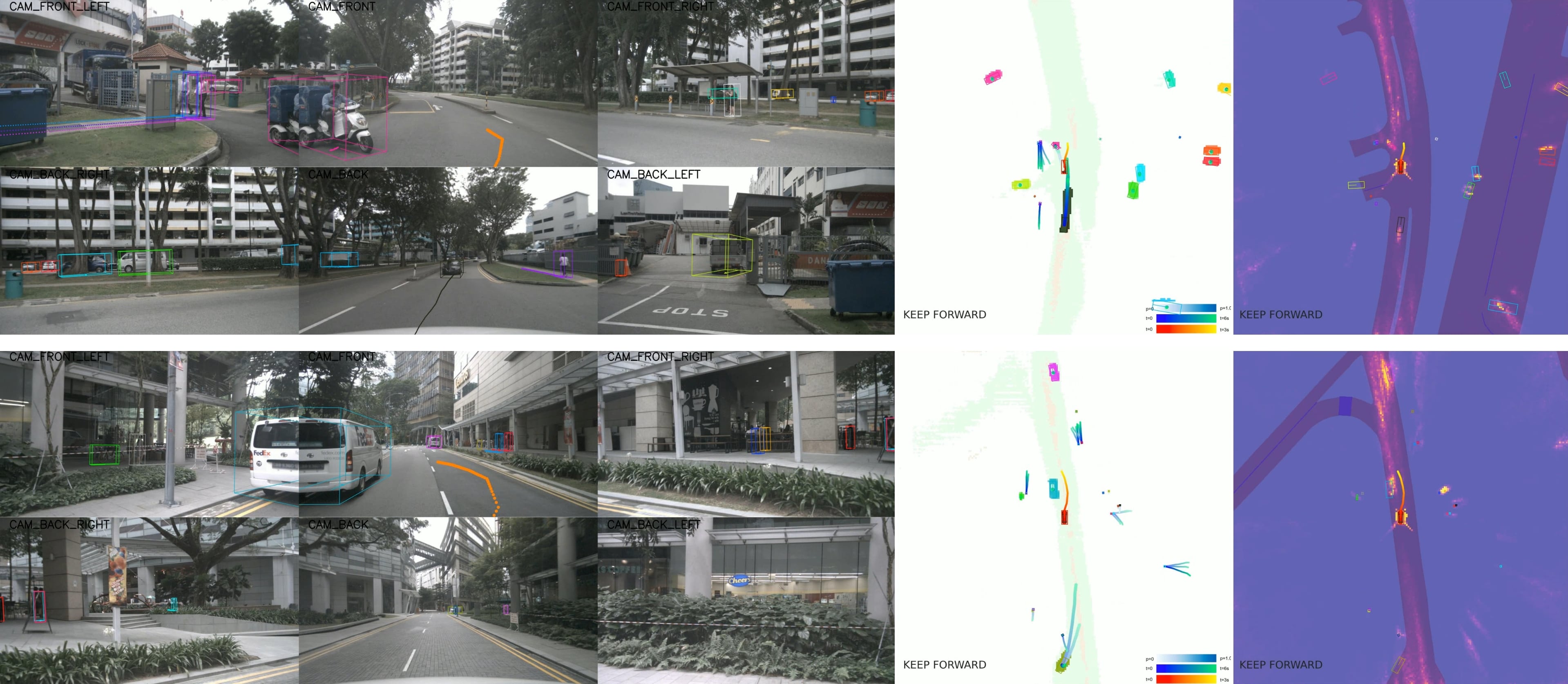
Figure 11: Obstacles avoidance visualization. In these two scenarios, the ego vehicle is changing lanes attentively to avoid the obstacle vehicle. From the attention mask, we can observe that our method focuses on the obstacles as well as the road in the front and back.

Figure 12: Visualization for planning recovering from perception failures. We show an interesting case where inaccurate results occur in prior modules while the later tasks could still recover. The top row and the down row represent two consecutive frames from the same scenario. The vehicle in the red circle is moving from a far distance toward the intersection at a high speed. It is observed that the tracking module misses it at first, then captures it at the latter frame. The blue circles show a stationary car yielding to the traffic, and it is missed in both frames. Interestingly, both vehicles show strong reactions to the attention masks of the planner, even though they are missed in the prior modules. It means that our planner still pays attention to those critical though missed agents, which is intractable in previous fragmented and non-unified driving systems, and demonstrates the robustness of UniAD.

Figure 13: Failure cases 1. Here we present a long-tail scenario, where a large trailer with a white container occupies the entire road. We can observe that our tracking module fails to detect the accurate size of the front trailer and heading angles of vehicles beside the road.

Figure 14: Failure cases 2. In this case, the planner is over-cautious about the incoming vehicle in the narrow street. The dark environment is one critical type of long-tail scenarios in autonomous driving. Applying smaller collision loss weight and more regulation regarding the boundary might mitigate the problem.

References

- [1] Adil Kaan Akan and Fatma Güney. StretchBEV: Stretching future instance prediction spatially and temporally. In ECCV, 2022.
- [2] Mayank Bansal, Alex Krizhevsky, and Abhijit Ogale. Chauffeurnet: Learning to drive by imitating the best and synthesizing the worst. arXiv preprint arXiv:1812.03079, 2018.
- [3] Hans Georg Bock and Karl-Josef Plitt. A multiple shooting algorithm for direct solution of optimal control problems. IFAC Proceedings Volumes, 1984.
- [4] Mariusz Bojarski, Davide Del Testa, Daniel Dworakowski, Bernhard Firner, Beat Flepp, Prasoon Goyal, Lawrence D Jackel, Mathew Monfort, Urs Muller, Jiakai Zhang, Xin Zhang, Jake Zhao, and Zieba Karol. End to end learning for self-driving cars. arXiv preprint arXiv:1604.07316, 2016.
- [5] Thibault Buhet, Émilie Wirbel, and Xavier Perrotton. PLOP: Probabilistic polynomial objects trajectory planning for autonomous driving. In CoRL, 2020.
- [6] Holger Caesar, Varun Bankiti, Alex H Lang, Sourabh Vora, Venice Erin Liong, Qiang Xu, Anush Krishnan, Yu Pan, Giancarlo Baldan, and Oscar Beijbom. nuscenes: A multimodal dataset for autonomous driving. In CVPR, 2020.
- [7] Holger Caesar, Juraj Kabzan, Kok Seang Tan, Whye Kit Fong, Eric Wolff, Alex Lang, Luke Fletcher, Oscar Beijbom, and Sammy Omari. nuplan: A closed-loop ml-based planning benchmark for autonomous vehicles. arXiv preprint arXiv:2106.11810, 2021.
- [8] Nicolas Carion, Francisco Massa, Gabriel Synnaeve, Nicolas Usunier, Alexander Kirillov, and Sergey Zagoruyko. End-to-end object detection with transformers. In ECCV, 2020.
- [9] Sergio Casas, Cole Gulino, Renjie Liao, and Raquel Urtasun. Spagnn: Spatially-aware graph neural networks for relational behavior forecasting from sensor data. In ICRA, 2020.
- [10] Sergio Casas, Wenjie Luo, and Raquel Urtasun. Intentnet: Learning to predict intention from raw sensor data. In CoRL, 2018.
- [11] Sergio Casas, Abbas Sadat, and Raquel Urtasun. Mp3: A unified model to map, perceive, predict and plan. In CVPR, 2021.
- [12] Yuning Chai, Benjamin Sapp, Mayank Bansal, and Dragomir Anguelov. Multipath: Multiple probabilistic anchor trajectory hypotheses for behavior prediction. In CoRL, 2020.
- [13] Raphael Chekroun, Marin Toromanoff, Sascha Hornauer, and Fabien Moutarde. GRI: General reinforced imitation and its application to vision-based autonomous driving. arXiv preprint 2111.08575, 2021.
- [14] Dian Chen, Vladlen Koltun, and Philipp Krähenbühl. Learning to drive from a world on rails. In ICCV, 2021.
- [15] Dian Chen and Philipp Krähenbühl. Learning from all vehicles. In CVPR, 2022.
- [16] Dian Chen, Brady Zhou, Vladlen Koltun, and Philipp Krähenbühl. Learning by cheating. In CoRL, 2020.
- [17] Bowen Cheng, Ishan Misra, Alexander G. Schwing, Alexander Kirillov, and Rohit Girdhar. Masked-attention mask transformer for universal image segmentation. In CVPR, 2022.
- [18] Bowen Cheng, Alex Schwing, and Alexander Kirillov. Per-pixel classification is not all you need for semantic segmentation. In NeurIPS, 2021.
- [19] Kashyap Chitta, Aditya Prakash, and Andreas Geiger. NEAT: Neural attention fields for end-to-end autonomous driving. In ICCV, 2021.
- [20] Kashyap Chitta, Aditya Prakash, Bernhard Jaeger, Zehao Yu, Katrin Renz, and Andreas Geiger. Transfuser: Imitation with transformer-based sensor fusion for autonomous driving. IEEE TPAMI, 2022.
- [21] Felipe Codevilla, Matthias Müller, Antonio López, Vladlen Koltun, and Alexey Dosovitskiy. End-to-end driving via conditional imitation learning. In ICRA, 2018.
- [22] Felipe Codevilla, Eder Santana, Antonio M López, and Adrien Gaidon. Exploring the limitations of behavior cloning for autonomous driving. In ICCV, 2019.
- [23] Michael Crawshaw. Multi-task learning with deep neural networks: A survey. arXiv preprint arXiv:2009.09796, 2020.
- [24] Alexander Cui, Sergio Casas, Abbas Sadat, Renjie Liao, and Raquel Urtasun. Lookout: Diverse multi-future prediction and planning for self-driving. In ICCV, 2021.
- [25] Nemanja Djuric, Henggang Cui, Zhaoen Su, Shangxuan Wu, Huahua Wang, Fang-Chieh Chou, Luisa San Martin, Song Feng, Rui Hu, Yang Xu, Alyssa Dayan, Sidney Zhang, Brian C. Becker, Gregory P. Meyer, Carlos Vallespi-Gonzalez, and Carl K. Wellington. Multixnet: Multiclass multistage multimodal motion prediction. In IV, 2021.
- [26] Alexey Dosovitskiy, German Ros, Felipe Codevilla, Antonio Lopez, and Vladlen Koltun. CARLA: An open urban driving simulator. In CoRL, 2017.
- [27] Scott Ettinger, Shuyang Cheng, Benjamin Caine, Chenxi Liu, Hang Zhao, Sabeek Pradhan, Yuning Chai, Ben Sapp, Charles R Qi, Yin Zhou, Zoey Yang, Aurélien Chouard, Pei Sun, Jiquan Ngiam, Vijay Vasudevan, Alexander McCauley, Jonathon Shlens, and Dragomir Anguelov. Large scale interactive motion forecasting for autonomous driving: The waymo open motion dataset. In ICCV, 2021.
- [28] Sudeep Fadadu, Shreyash Pandey, Darshan Hegde, Yi Shi, Fang-Chieh Chou, Nemanja Djuric, and Carlos Vallespi-Gonzalez. Multi-view fusion of sensor data for improved perception and prediction in autonomous driving. In WACV, 2022.
- [29] Jiyang Gao, Chen Sun, Hang Zhao, Yi Shen, Dragomir Anguelov, Congcong Li, and Cordelia Schmid. Vectornet: Encoding hd maps and agent dynamics from vectorized representation. In CVPR, 2020.
- [30] Junru Gu, Chenxu Hu, Tianyuan Zhang, Xuanyao Chen, Yilun Wang, Yue Wang, and Hang Zhao. ViP3D: End-to-end visual trajectory prediction via 3d agent queries. In CVPR, 2023.
- [31] Chunrui Han, Jianjian Sun, Zheng Ge, Jinrong Yang, Runpei Dong, Hongyu Zhou, Weixin Mao, Yuang Peng, and Xiangyu Zhang. Exploring recurrent long-term temporal fusion for multi-view 3d perception. arXiv preprint arXiv:2303.05970, 2023.
- [32] Kaiming He, Xiangyu Zhang, Shaoqing Ren, and Jian Sun. Deep residual learning for image recognition. In CVPR, 2016.
- [33] Noureldin Hendy, Cooper Sloan, Feng Tian, Pengfei Duan, Nick Charchut, Yuesong Xie, Chuang Wang, and James Philbin. Fishing net: Future inference of semantic heatmaps in grids. arXiv preprint arXiv:2006.09917, 2020.
- [34] Anthony Hu, Gianluca Corrado, Nicolas Griffiths, Zak Murez, Corina Gurau, Hudson Yeo, Alex Kendall, Roberto Cipolla, and Jamie Shotton. Model-based imitation learning for urban driving. In NeurIPS, 2022.
- [35] Anthony Hu, Zak Murez, Nikhil Mohan, Sofía Dudas, Jeffrey Hawke, Vijay Badrinarayanan, Roberto Cipolla, and Alex Kendall. FIERY: Future instance prediction in bird’s-eye view from surround monocular cameras. In ICCV, 2021.
- [36] Hou-Ning Hu, Yung-Hsu Yang, Tobias Fischer, Trevor Darrell, Fisher Yu, and Min Sun. Monocular quasi-dense 3d object tracking. IEEE TPAMI, 2022.
- [37] Peiyun Hu, Aaron Huang, John Dolan, David Held, and Deva Ramanan. Safe local motion planning with self-supervised freespace forecasting. In CVPR, 2021.
- [38] Shengchao Hu, Li Chen, Penghao Wu, Hongyang Li, Junchi Yan, and Dacheng Tao. ST-P3: End-to-end vision-based autonomous driving via spatial-temporal feature learning. In ECCV, 2022.
- [39] Zhiyu Huang, Haochen Liu, Jingda Wu, and Chen Lv. Differentiable integrated motion prediction and planning with learnable cost function for autonomous driving. arXiv preprint arXiv:2207.10422, 2022.
- [40] Boris Ivanovic, Amine Elhafsi, Guy Rosman, Adrien Gaidon, and Marco Pavone. MATS: An interpretable trajectory forecasting representation for planning and control. In CoRL, 2021.
- [41] Xiaosong Jia, Li Chen, Penghao Wu, Jia Zeng, Junchi Yan, Hongyang Li, and Yu Qiao. Towards capturing the temporal dynamics for trajectory prediction: a coarse-to-fine approach. In CoRL, 2022.
- [42] Xiaosong Jia, Liting Sun, Masayoshi Tomizuka, and Wei Zhan. Ide-net: Interactive driving event and pattern extraction from human data. IEEE RA-L, 2021.
- [43] Xiaosong Jia, Liting Sun, Hang Zhao, Masayoshi Tomizuka, and Wei Zhan. Multi-agent trajectory prediction by combining egocentric and allocentric views. In CoRL, 2021.
- [44] Xiaosong Jia, Penghao Wu, Li Chen, Hongyang Li, Yu Liu, and Junchi Yan. HDGT: Heterogeneous driving graph transformer for multi-agent trajectory prediction via scene encoding. arXiv preprint arXiv:2205.09753, 2022.
- [45] Alexey Kamenev, Lirui Wang, Ollin Boer Bohan, Ishwar Kulkarni, Bilal Kartal, Artem Molchanov, Stan Birchfield, David Nistér, and Nikolai Smolyanskiy. Predictionnet: Real-time joint probabilistic traffic prediction for planning, control, and simulation. In ICRA, 2022.
- [46] Alex Kendall, Jeffrey Hawke, David Janz, Przemyslaw Mazur, Daniele Reda, John-Mark Allen, Vinh-Dieu Lam, Alex Bewley, and Amar Shah. Learning to drive in a day. In ICRA, 2019.
- [47] Tarasha Khurana, Peiyun Hu, Achal Dave, Jason Ziglar, David Held, and Deva Ramanan. Differentiable raycasting for self-supervised occupancy forecasting. In ECCV, 2022.
- [48] Dahun Kim, Sanghyun Woo, Joon-Young Lee, and In So Kweon. Video panoptic segmentation. In CVPR, 2020.
- [49] Jinkyu Kim, Reza Mahjourian, Scott Ettinger, Mayank Bansal, Brandyn White, Ben Sapp, and Dragomir Anguelov. Stopnet: Scalable trajectory and occupancy prediction for urban autonomous driving. arXiv preprint arXiv:2206.00991, 2022.
- [50] Alexander Kirillov, Kaiming He, Ross Girshick, Carsten Rother, and Piotr Dollár. Panoptic segmentation. In CVPR, 2019.
- [51] Youngwan Lee, Joong-won Hwang, Sangrok Lee, Yuseok Bae, and Jongyoul Park. An energy and gpu-computation efficient backbone network for real-time object detection. In CVPR Workshop, 2019.
- [52] Feng Li, Hao Zhang, Shilong Liu, Lei Zhang, Lionel M Ni, and Heung-Yeung Shum. Mask dino: Towards a unified transformer-based framework for object detection and segmentation. In CVPR, 2023.
- [53] Lingyun Luke Li, Bin Yang, Ming Liang, Wenyuan Zeng, Mengye Ren, Sean Segal, and Raquel Urtasun. End-to-end contextual perception and prediction with interaction transformer. In IROS, 2020.
- [54] Yanwei Li, Yilun Chen, Xiaojuan Qi, Zeming Li, Jian Sun, and Jiaya Jia. Unifying voxel-based representation with transformer for 3d object detection. In NeurIPS, 2022.
- [55] Zhiqi Li, Wenhai Wang, Hongyang Li, Enze Xie, Chonghao Sima, Tong Lu, Qiao Yu, and Jifeng Dai. BEVFormer: Learning bird’s-eye-view representation from multi-camera images via spatiotemporal transformers. In ECCV, 2022.
- [56] Zhiqi Li, Wenhai Wang, Enze Xie, Zhiding Yu, Anima Anandkumar, Jose M Alvarez, Ping Luo, and Tong Lu. Panoptic segformer: Delving deeper into panoptic segmentation with transformers. In CVPR, 2022.
- [57] Ming Liang, Bin Yang, Wenyuan Zeng, Yun Chen, Rui Hu, Sergio Casas, and Raquel Urtasun. Pnpnet: End-to-end perception and prediction with tracking in the loop. In CVPR, 2020.
- [58] Tingting Liang, Hongwei Xie, Kaicheng Yu, Zhongyu Xia, Zhiwei Lin, Yongtao Wang, Tao Tang, Bing Wang, and Zhi Tang. BEVFusion: A simple and robust lidar-camera fusion framework. In NeurIPS, 2022.
- [59] Xiaodan Liang, Tairui Wang, Luona Yang, and Eric Xing. Cirl: Controllable imitative reinforcement learning for vision-based self-driving. In ECCV, 2018.
- [60] Xiwen Liang, Yangxin Wu, Jianhua Han, Hang Xu, Chunjing Xu, and Xiaodan Liang. Effective adaptation in multi-task co-training for unified autonomous driving. In NeurIPS, 2022.
- [61] Tsung-Yi Lin, Priya Goyal, Ross Girshick, Kaiming He, and Piotr Dollár. Focal loss for dense object detection. In ICCV, 2017.
- [62] Jerry Liu, Wenyuan Zeng, Raquel Urtasun, and Ersin Yumer. Deep structured reactive planning. In ICRA, 2021.
- [63] Yicheng Liu, Jinghuai Zhang, Liangji Fang, Qinhong Jiang, and Bolei Zhou. Multimodal motion prediction with stacked transformers. In CVPR, 2021.
- [64] Zhijian Liu, Haotian Tang, Alexander Amini, Xingyu Yang, Huizi Mao, Daniela Rus, and Song Han. BEVFusion: Multi-task multi-sensor fusion with unified bird’s-eye view representation. In ICRA, 2023.
- [65] Ilya Loshchilov and Frank Hutter. Decoupled weight decay regularization. In ICLR, 2018.
- [66] Wenjie Luo, Bin Yang, and Raquel Urtasun. Fast and furious: Real time end-to-end 3d detection, tracking and motion forecasting with a single convolutional net. In CVPR, 2018.
- [67] Fausto Milletari, Nassir Navab, and Seyed-Ahmad Ahmadi. V-net: Fully convolutional neural networks for volumetric medical image segmentation. In 3DV, 2016.
- [68] Mobileye. Mobileye under the hood. https://www.mobileye.com/ces-2022/, 2022.
- [69] Nigamaa Nayakanti, Rami Al-Rfou, Aurick Zhou, Kratarth Goel, Khaled S Refaat, and Benjamin Sapp. Wayformer: Motion forecasting via simple & efficient attention networks. arXiv preprint arXiv:2207.05844, 2022.
- [70] Jiquan Ngiam, Benjamin Caine, Vijay Vasudevan, Zhengdong Zhang, Hao-Tien Lewis Chiang, Jeffrey Ling, Rebecca Roelofs, Alex Bewley, Chenxi Liu, Ashish Venugopal, David Weiss, Ben Sapp, Zhifeng Chen, and Jonathon Shlens. Scene transformer: A unified multi-task model for behavior prediction and planning. In ICLR, 2022.
- [71] Nvidia. NVIDIA DRIVE End-to-End Solutions for Autonomous Vehicles. https://developer.nvidia.com/drive, 2022.
- [72] Bowen Pan, Jiankai Sun, Ho Yin Tiga Leung, Alex Andonian, and Bolei Zhou. Cross-view semantic segmentation for sensing surroundings. IEEE RA-L, 2020.
- [73] Dennis Park, Rares Ambrus, Vitor Guizilini, Jie Li, and Adrien Gaidon. Is pseudo-lidar needed for monocular 3d object detection? In ICCV, 2021.
- [74] Jinhyung Park, Chenfeng Xu, Shijia Yang, Kurt Keutzer, Kris Kitani, Masayoshi Tomizuka, and Wei Zhan. Time will tell: New outlooks and a baseline for temporal multi-view 3d object detection. arXiv preprint arXiv:2210.02443, 2022.
- [75] Neehar Peri, Jonathon Luiten, Mengtian Li, Aljoša Ošep, Laura Leal-Taixé, and Deva Ramanan. Forecasting from lidar via future object detection. In CVPR, 2022.
- [76] Jonah Philion and Sanja Fidler. Lift, splat, shoot: Encoding images from arbitrary camera rigs by implicitly unprojecting to 3d. In ECCV, 2020.
- [77] Dean A Pomerleau. Alvinn: An autonomous land vehicle in a neural network. In NeurIPS, 1988.
- [78] Aditya Prakash, Kashyap Chitta, and Andreas Geiger. Multi-modal fusion transformer for end-to-end autonomous driving. In CVPR, 2021.
- [79] Scott Reed, Konrad Zolna, Emilio Parisotto, Sergio Gomez Colmenarejo, Alexander Novikov, Gabriel Barth-Maron, Mai Gimenez, Yury Sulsky, Jackie Kay, Jost Tobias Springenberg, Tom Eccles, Jake Bruce, Ali Razavi, Ashley Edwards, Nicolas Heess, Yutian Chen, Raia Hadsell, Oriol Vinyals, Mahyar Bordbar, and Nando de Freitas. A generalist agent. arXiv preprint arXiv:2205.06175, 2022.
- [80] Hamid Rezatofighi, Nathan Tsoi, JunYoung Gwak, Amir Sadeghian, Ian Reid, and Silvio Savarese. Generalized intersection over union: A metric and a loss for bounding box regression. In CVPR, 2019.
- [81] Nicholas Rhinehart, Rowan McAllister, Kris Kitani, and Sergey Levine. PRECOG: Prediction conditioned on goals in visual multi-agent settings. In ICCV, 2019.
- [82] Abbas Sadat, Sergio Casas, Mengye Ren, Xinyu Wu, Pranaab Dhawan, and Raquel Urtasun. Perceive, predict, and plan: Safe motion planning through interpretable semantic representations. In ECCV, 2020.
- [83] Hao Shao, Letian Wang, Ruobing Chen, Hongsheng Li, and Yu Liu. Safety-enhanced autonomous driving using interpretable sensor fusion transformer. In CoRL, 2022.
- [84] Shaoshuai Shi, Li Jiang, Dengxin Dai, and Bernt Schiele. Motion transformer with global intention localization and local movement refinement. In NeurIPS, 2022.
- [85] Yining Shi, Jingyan Shen, Yifan Sun, Yunlong Wang, Jiaxin Li, Shiqi Sun, Kun Jiang, and Diange Yang. Srcn3d: Sparse r-cnn 3d surround-view camera object detection and tracking for autonomous driving. arXiv preprint arXiv:2206.14451, 2022.
- [86] Haoran Song, Wenchao Ding, Yuxuan Chen, Shaojie Shen, Michael Yu Wang, and Qifeng Chen. Pip: Planning-informed trajectory prediction for autonomous driving. In ECCV, 2020.
- [87] Tesla. Tesla AI Day. https://www.youtube.com/watch?v=ODSJsviD_SU, 2022.
- [88] Sebastian Thrun and Arno Bücken. Integrating grid-based and topological maps for mobile robot navigation. In AAAI, 1996.
- [89] Marin Toromanoff, Emilie Wirbel, and Fabien Moutarde. End-to-end model-free reinforcement learning for urban driving using implicit affordances. In CVPR, 2020.
- [90] Balakrishnan Varadarajan, Ahmed Hefny, Avikalp Srivastava, Khaled S Refaat, Nigamaa Nayakanti, Andre Cornman, Kan Chen, Bertrand Douillard, Chi Pang Lam, Dragomir Anguelov, and Benjamin Sapp. Multipath++: Efficient information fusion and trajectory aggregation for behavior prediction. arXiv preprint arXiv:2111.14973, 2021.
- [91] Ashish Vaswani, Noam Shazeer, Niki Parmar, Jakob Uszkoreit, Llion Jones, Aidan N Gomez, Łukasz Kaiser, and Illia Polosukhin. Attention is all you need. In NeurIPS, 2017.
- [92] Peng Wang, An Yang, Rui Men, Junyang Lin, Shuai Bai, Zhikang Li, Jianxin Ma, Chang Zhou, Jingren Zhou, and Hongxia Yang. Ofa: Unifying architectures, tasks, and modalities through a simple sequence-to-sequence learning framework. In ICML, 2022.
- [93] Qitai Wang, Yuntao Chen, Ziqi Pang, Naiyan Wang, and Zhaoxiang Zhang. Immortal tracker: Tracklet never dies. arXiv preprint arXiv:2111.13672, 2021.
- [94] Bob Wei, Mengye Ren, Wenyuan Zeng, Ming Liang, Bin Yang, and Raquel Urtasun. Perceive, attend, and drive: Learning spatial attention for safe self-driving. In ICRA, 2021.
- [95] Penghao Wu, Li Chen, Hongyang Li, Xiaosong Jia, Junchi Yan, and Yu Qiao. Policy pre-training for autonomous driving via self-supervised geometric modeling. In ICLR, 2023.
- [96] Pengxiang Wu, Siheng Chen, and Dimitris N Metaxas. Motionnet: Joint perception and motion prediction for autonomous driving based on bird’s eye view maps. In CVPR, 2020.
- [97] Penghao Wu, Xiaosong Jia, Li Chen, Junchi Yan, Hongyang Li, and Yu Qiao. Trajectory-guided control prediction for end-to-end autonomous driving: A simple yet strong baseline. In NeurIPS, 2022.
- [98] Jinrong Yang, En Yu, Zeming Li, Xiaoping Li, and Wenbing Tao. Quality matters: Embracing quality clues for robust 3d multi-object tracking. arXiv preprint arXiv:2208.10976, 2022.
- [99] Ye Yuan, Xinshuo Weng, Yanglan Ou, and Kris M Kitani. Agentformer: Agent-aware transformers for socio-temporal multi-agent forecasting. In ICCV, 2021.
- [100] Fangao Zeng, Bin Dong, Tiancai Wang, Xiangyu Zhang, and Yichen Wei. Motr: End-to-end multiple-object tracking with transformer. In ECCV, 2021.
- [101] Wenyuan Zeng, Wenjie Luo, Simon Suo, Abbas Sadat, Bin Yang, Sergio Casas, and Raquel Urtasun. End-to-end interpretable neural motion planner. In CVPR, 2019.
- [102] Wenyuan Zeng, Shenlong Wang, Renjie Liao, Yun Chen, Bin Yang, and Raquel Urtasun. Dsdnet: Deep structured self-driving network. In ECCV, 2020.
- [103] Jimuyang Zhang and Eshed Ohn-Bar. Learning by watching. In CVPR, 2021.
- [104] Tianyuan Zhang, Xuanyao Chen, Yue Wang, Yilun Wang, and Hang Zhao. MUTR3D: A Multi-camera Tracking Framework via 3D-to-2D Queries. In CVPR Workshop, 2022.
- [105] Yunpeng Zhang, Zheng Zhu, Wenzhao Zheng, Junjie Huang, Guan Huang, Jie Zhou, and Jiwen Lu. BEVerse: Unified perception and prediction in birds-eye-view for vision-centric autonomous driving. arXiv preprint arXiv:2205.09743, 2022.
- [106] Zhejun Zhang, Alexander Liniger, Dengxin Dai, Fisher Yu, and Luc Van Gool. End-to-end urban driving by imitating a reinforcement learning coach. In ICCV, 2021.
- [107] Hang Zhao, Jiyang Gao, Tian Lan, Chen Sun, Benjamin Sapp, Balakrishnan Varadarajan, Yue Shen, Yi Shen, Yuning Chai, Cordelia Schmid, Congcong Li, and Dragomir Anguelov. TNT: Target-driven trajectory prediction. In CoRL, 2020.
- [108] Jinguo Zhu, Xizhou Zhu, Wenhai Wang, Xiaohua Wang, Hongsheng Li, Xiaogang Wang, and Jifeng Dai. Uni-perceiver-moe: Learning sparse generalist models with conditional moes. In NeurIPS, 2022.
- [109] Xizhou Zhu, Weijie Su, Lewei Lu, Bin Li, Xiaogang Wang, and Jifeng Dai. Deformable detr: Deformable transformers for end-to-end object detection. In ICLR, 2020.