The AstroSat observation of accreting millisecond X-ray pulsar SAX J1808.4-3658 during its 2019 outburst

Abstract

We report on the analysis of the AstroSat dataset of the accreting millisecond X-ray pulsar SAX J1808.4-3658, obtained during its 2019 outburst. We found coherent pulsations at $\sim 401$ Hz and an orbital solution consistent with previous studies. The 3–20 keV pulse profile can be well fitted with three harmonically related sinusoidal components with background-corrected fractional amplitude of $\sim 3.5\%$, $\sim 1.2\%$ and $\sim 0.37\%$ for fundamental, second and third harmonic, respectively. Our energy-resolved pulse profile evolution study indicate a strong energy dependence. We also observed a soft lag in fundamental and hard lag during its harmonic. The broadband spectrum of SAX J1808.4-3658 can be well described with a combination of thermal emission component with $kT\sim 1$ keV, a thermal Comptonization ($\Gamma\sim 1.67$) from the hot corona and broad emission lines due to Fe.

1 Introduction

SAX J1808.4-3658 was the first X-ray binary to show millisecond X-ray pulsations at $\sim 401$ Hz in a $\sim 2$ hr compact binary orbit (Wijnands & van der Klis, 1998a; Chakrabarty & Morgan, 1998). Since then, 25 such sources with milliseconds pulsations have been discovered (e.g., Di Salvo & Sanna, 2020; Ng et al., 2021; Bult et al., 2022; Sanna et al., 2022b). These systems are generally referred as Accretion-powered Millisecond X-ray Pulsars (AMXPs) (see e.g., Patruno & Watts, 2012; Campana & Di Salvo, 2018; Di Salvo & Sanna, 2020, for reviews). These systems are transient in nature and observed during outburst phases. AMXPs are a sub-class of low-mass X-ray binaries (LMXBs; Charles, 2011) where companion’s mass is $\lesssim 1M_{\sun}$.

The magnetic field of AMXPs have been estimated to be of the order of $\sim 10^{8}-10^{9}$ G (see e.g., Cackett et al., 2009; Mukherjee et al., 2015; Ludlam et al., 2017; Pan et al., 2018; Sharma et al., 2020, Beri et al. 2022 submitted), strong enough to channel at-least part of the accretion stream to the magnetic poles which results in X-ray modulation at Neutron Star (NS) spin. The X-ray spectrum of AMXPs can be well modelled with thermal emission from an accretion disc and/or NS surface, thermal Comptonization and reprocessed emission from the accretion disc in form of reflection spectrum (e.g., Cackett et al., 2009; Cackett et al., 2010; Papitto et al., 2009, 2010, 2013; Pintore et al., 2016; Di Salvo et al., 2019; Sharma et al., 2019). They mostly show the hard spectral state with some exceptions (Sharma et al., 2019; Di Salvo & Sanna, 2020, Beri et al. 2022 submitted) where they show spectral state transition between the hard and soft spectral states similar to atoll sources (e.g. Hasinger & van der Klis, 1989).

Since 1996, SAX J1808.4-3658 has been frequently observed in outburst every 2.5–4 years. A total of ten outbursts (in 1996, 1998, 2000, 2002, 2005, 2008, 2011, 2015, 2019 and 2022) have been observed. Over the last two decades, SAX J1808.4-3658 has been studied extensively. Aspects of coherent pulsations (Poutanen & Gierliński, 2003; Jain et al., 2007; Hartman et al., 2008; Burderi et al., 2009; Patruno et al., 2017; Sanna et al., 2017; Bult et al., 2020), spectral characteristics (Gierliński et al., 2002; Cackett et al., 2009; Papitto et al., 2009; Di Salvo et al., 2019), thermonuclear X-ray bursts (in ’t Zand et al., 1998; Galloway & Cumming, 2006; Bhattacharyya & Strohmayer, 2007; Bult et al., 2019a) and aperiodic and quasi-periodic variability (Wijnands & van der Klis, 1998b; Wijnands et al., 2003; van Straaten et al., 2005; Patruno et al., 2009c; Bult & van der Klis, 2015) have been deeply investigated. The properties of source have also been deeply investigated during quiescence and outburst in multi-wavelength (e.g., Radio, Optical, UV, etc. Gaensler et al., 1999; Wang et al., 2001; Wang et al., 2013; Cornelisse et al., 2009; Heinke et al., 2009; Patruno et al., 2017; Tudor et al., 2017; Baglio et al., 2020; Goodwin et al., 2020; Ambrosino et al., 2021).

The 2019 outburst of SAX J1808.4-3658 started around August 6, 2019 (Bult et al., 2019b; Goodwin et al., 2019; Parikh & Wijnands, 2019) which lasted about a month. After episodes of reflaring, source went back into quiescence state (Baglio et al., 2019b; Baglio et al., 2019a; Bult et al., 2019c), similar to its previous outbursts (Patruno et al., 2016). Twelve days before the on-set of outburst, enhancement in the optical flux was observed (Russell et al., 2019; Goodwin et al., 2020). Neutron Star Interior Composition Explorer (NICER; Gendreau & Arzoumanian, 2017) monitored the 2019 outburst from start to the reflaring states. Bult et al. (2020) performed the coherent timing analysis using NICER observations during the outburst of 2019, and found a secular spin-down of the pulsar at rate of $1.01(7)\times 10^{-15}$ Hz s^-1. A very bright Photospheric Radius Expansion (PRE) burst with NICER was also observed (Bult et al., 2019a). Coherent pulsations in optical and ultraviolet were detected at $\sim 401$ Hz likely to be driven by synchro-curvature radiation in the pulsar magnetosphere or just outside of it (Ambrosino et al., 2021). Recently, SAX J1808.4-3658 was again observed in the outburst in August 2022 (Sanna et al., 2022c).

During the 2019 outburst, we also observed SAX J1808.4-3658 with AstroSat mission under Target of Opportunity (ToO). According to NICER observations, the outburst reached its peak on August 13 (MJD 58708), after which it started to decay (Bult et al., 2019c). The AstroSat observation was carried out just after the peak of the outburst (see, Figure 1). In this work, we report for the first time the results from the timing analysis carried out with AstroSat/LAXPC data and the spectroscopy performed using SXT and LAXPC data.

2 Observations and data analysis

Table 1: Log of X-ray observations.

Instrument	OBS ID	Start Time		Stop Time		Mode	Obs span
		(YY-MM-DD HH:MM:SS)	MJD	(YY-MM-DD HH:MM:SS)	MJD		(ks)
AstroSat/LAXPC	9000003090	2019-08-14 01:10:46	58709.04914	2019-08-15 09:56:53	58710.41450	EA	118
AstroSat/SXT	9000003090	2019-08-14 02:19:02	58709.09655	2019-08-15 10:30:16	58710.43768	PC	116

Figure 1: The 0.5–10 keV NICER lightcurve of SAX J1808.4-3658 during its 2019 outburst. The two vertical red lines represent the time range of the AstroSat observation.

AstroSat is India’s first dedicated multi-wavelength astronomy satellite (Agrawal, 2006; Singh et al., 2014), launched in 2015. It has five principal payloads on-board: (i) the Soft X-ray Telescope (SXT), (ii) the Large Area X-ray Proportional Counters (LAXPCs), (iii) the Cadmium-Zinc-Telluride Imager (CZTI), (iv) the Ultra-Violet Imaging Telescope (UVIT), and (v) the Scanning Sky Monitor (SSM). Table 1 gives the log of observations that have been used in this work. We analysed data from SXT and LAXPC only.

2.1 AstroSat/LAXPC

LAXPC is one of the primary instrument aboard AstroSat. It consists of three co-aligned identical proportional counters (LAXPC10, LAXPC20 and LAXPC30) that work in the energy range of 3–80 keV. Each LAXPC detector independently record the arrival time of each photon with a time resolution of $10~{}\mu$s and has five layers (for details see Yadav et al., 2016; Antia et al., 2017).

As LAXPC10 was operating at low gain and detector LAXPC30 was switched off during the observation, we used only LAXPC20 detector for our analysis. We used the data collected in the Event Analysis (EA) mode and processed using LaxpcSoft version 3.1.1 software package to extract light curves and spectra. LAXPC detectors have dead-time of $42~{}\mu$s and the extracted products are dead-time corrected. The background in LAXPC is estimated from the blank sky observations (see Antia et al., 2017, for details). To minimize the background, we have performed all analysis using the data from top layer (L1, L2) of LAXPC20 detector. We have used corresponding response files to obtain channel to energy conversion information while performing energy-resolved analysis.

We corrected the LAXPC photon arrival times to the Solar system barycentre by using the as1bary tool. We used the best available position of the source, R.A. (J2000)$=18^{h}08^{m}27.647^{s}$ and Dec. (J2000) $=-36^{\circ}58^{\prime}43.90^{\prime\prime}$ obtained through pulsar timing astrometry (Bult et al., 2020).

2.2 AstroSat/SXT

The Soft X-ray Telescope (SXT) is a focusing X-ray telescope with CCD in the focal plane that can perform X-ray imaging and spectroscopy in the 0.3–7 keV energy range (Singh et al., 2016; Singh et al., 2017). SAX J1808.4-3658 was observed in the Photon Counting (PC) mode with SXT (Table 1). Level 1 data were processed with AS1SXTLevel2-1.4b pipeline software to produce level 2 clean event files. The level 2 cleaned files from each orbits were merged using SXT Event Merger Tool (Julia Code). This merged event file was then used to extract image, light curves and spectra using the ftool task xselect, provided as part of heasoft version 6.29. A circular region with radius of 15 arcmin centered on the source was used. For spectral analysis, we have used the blank sky SXT spectrum as background (SkyBkg_comb_EL3p5_Cl_Rd16p0_v01.pha) and spectral redistribution matrix file (sxt_pc_mat_g0to12.rmf) provided by the SXT team. We generated the correct off-axis auxiliary response files (ARF) using sxtARFModule tool from the on-axis ARF (sxt_pc_excl00_v04_20190608.arf) provided by the SXT instrument team.

Figure 2: The top two panels show background corrected light curve from LAXPC20 binned at 100 sec in energy range of 3–10 keV and 10–30 keV, respectively. The bottom shows the hardness ratio (=10–30 keV/3–10 keV) binned at 100 sec.

3 Results

3.1 Light Curve

Fig. 1 shows the light curve of SAX J1808.4-3658 during its 2019 outburst as observed with NICER. The AstroSat observation (red vertical lines) was carried out near the peak of the outburst. Fig. 2 shows the background corrected light curve extracted from LAXPC20 binned at 100 sec in two different energy bands 3–10 keV (top panel) and 10–30 keV (middle panel). The LAXPC light curves show the persistent emission separated by data gaps due to Earth occultation and South Atlantic Anomaly (SAA) passage. No type-I X-ray burst was observed during the observation. The bottom panel presents the hardness ratio calculated using light curves in the two energy bands 3–10 keV and 10–30 keV. As hardness ratio is observed to be constant during the observation, this suggests that source did not seem to change spectral state within the observation duration.

3.2 Aperiodic Timing

We created the power density spectrum (PDS) using LAXPC20 event data-set in the 3–20 keV energy range. We binned the data at 0.5 ms to have Nyquist frequency of 1000 Hz and used $\sim 262$ sec segments to calculate the Fourier transform. All power spectra were averaged and rebinned geometrically with factor of 1.05. No background correction was applied. The power spectra was calculated using rms normalization and Poisson noise was subtracted using ftool powspec norm=-2. The PDS of X-ray binaries can be described in terms of a sum of Lorentzian functions (e.g., Nowak, 2000; Belloni et al., 2002). The Lorentzian profile is a function of frequency and can be defined as

$$P(\nu)=\frac{r^{2}\Delta}{2\pi}\frac{1}{(\nu-\nu_{0})^{2}+(\Delta/2)^{2}},$$ (1)

where $\nu_{0}$ is the centroid frequency, $\Delta$ is the full-width at half-maximum (FWHM), and $r$ is the integrated fractional rms. The quality factor of Lorentzian $Q=\nu_{0}/\Delta$ used to differentiate if a feature is a Quasi-Periodic Oscillations (QPO) or noise. The components with $Q>2$ are generally considered as QPOs, otherwise band-limited noise (e.g., Belloni et al., 2002; van der Klis, 2004; Bult & van der Klis, 2015).

Figure 3: Power density spectrum of SAX J1808.4-3658 in the 3–20 keV energy range. The PDS is rms normalized and white noise subtracted. Three Lorentzian functions are used to model the PDS in 0.004–200 Hz.

Table 2: The best-fit of the PDS. Reported errors are at $1\sigma$ confidence level for single parameter.

Component	1	2	3
Freq., $\nu_{0}$ (Hz)	$0.1675_{-0.016}^{+0.015}$	$3.33_{-0.74}^{+0.37}$	$17.1_{-6.3}^{+5.6}$
FWHM, $\Delta$ (Hz)	$0.96\pm 0.05$	$5.7_{-1.5}^{+2.1}$	$39.6_{-6.4}^{+7.2}$
Ch. Freq., $\nu_{\rm max}$ (Hz)	$0.508$	$4.38$	$26.16$
rms (%)	$17.5^{+0.3}_{-0.4}$	$11.0_{-1.4}^{+1.8}$	$13.2\pm 1.2$
$\chi^{2}/{\rm dof}$		175/151

SAX J1808.4-3658 is known to show peaked noise, low-frequency QPOs and kHz QPOs (e.g., Wijnands & van der Klis, 1998b; Wijnands et al., 2003; van Straaten et al., 2005; Patruno et al., 2009c; Bult & van der Klis, 2015). Fig. 3 shows the PDS of SAX J1808.4-3658 from LAXPC20 in 0.004–200 Hz, as no significant power is observed above 200 Hz. It shows only the red noise and no low-frequency QPO was observed. The PDS can be well modelled with combination of three Lorentzian functions (see, Table 2). Generally, each Lorentzian of the noise component can be expressed with characteristic frequency $\nu_{\rm max}=\sqrt{\nu_{0}^{2}+(\Delta/2)^{2}}$ and fractional rms amplitude (Belloni et al., 2002; Bult & van der Klis, 2015). We found the $\nu_{\rm max}$ of $\sim$ 0.5, 4.4, 26 Hz and rms of $\sim$ 17.5, 11, 13 % of the three Lorentzians, respectively.

3.3 Coherent Timing analysis

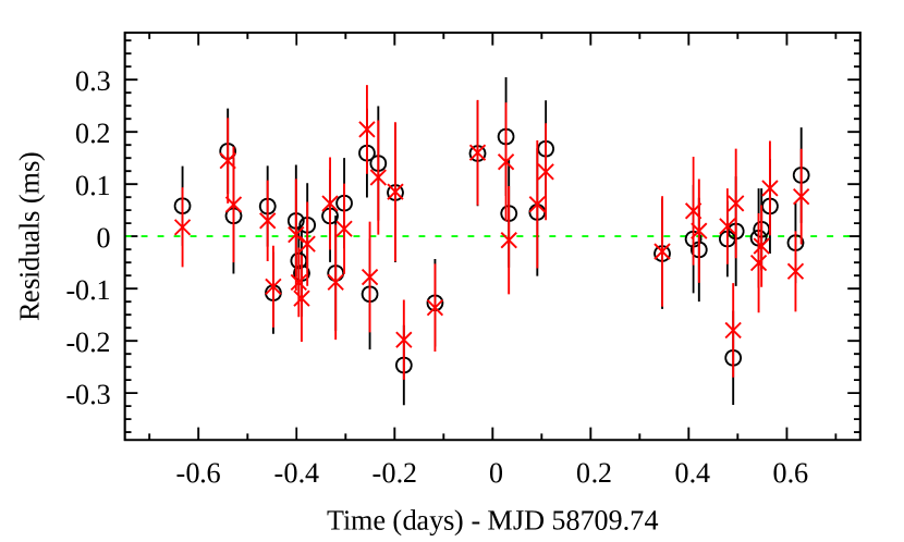
Figure 4: The residuals obtained from fitting the pulse phase delays of the fundamental component. Red cross points represents the residuals with equation 3 (quadratic+orbital) and black circles represents the residuals with only quadratic function ($R_{\rm orb}(t)=0$).

The pulses from rotating NS can lose coherence within a relatively short timescale due to Doppler modulations of arrival time of pulses in short orbital period of $\sim 2$ hr. In addition, the small pulse fraction can also makes it difficult to detect pulse arrival times from small segments of the light curve. Therefore, to detect the pulsations or true spin frequency during these observations, the light curve should be corrected for the binary motion. So, we corrected the photon time of arrivals of the AstroSat/LAXPC data-set for the delays caused by the binary motion. The delay induced by the orbital motion can be written as (Burderi et al., 2007):

$$\frac{z(t)}{c}=\frac{a_{x}\sin i}{c}\,\sin\Big{(}\frac{2\pi}{P_{\rm orb}}\,(t-T^{\star})\Big{)},$$ (2)

where $a_{x}\sin{\textit{i}/c}$ is the projected semi-major axis of the NS orbit in light seconds, $P_{\rm orb}$ is the orbital period, and $T^{\star}$ is the time of passage from the ascending node.

Bult et al. (2020) found the latest updated orbital solution at the outburst of 2019 using NICER observations. Therefore, we corrected photon time of arrivals adopting the 2019 orbital ephemeris reported in Bult et al. (2020). We then applied epoch-folding techniques to search for X-ray pulsation around the spin frequency value $\nu_{0}$ = 400.97520983 Hz, corresponding to the spin frequency measured during the same outburst with NICER (Bult et al., 2020). We used 16 phase bins to sample the signal. We explored the frequency space with steps of $10^{-8}$ Hz for a total of 10001 steps. The most significant pulse profile was been obtained for an average local spin frequency of $\bar{\nu}=400.97520994$ Hz.

We also investigated the evolution of the pulse phase delays. We divided the data in time intervals of $\sim 500$ sec and epoch-folded each segment in $8$ phase bins at the mean spin frequency $\bar{\nu}$ with respect to the epoch $T_{0}=58709.74$ MJD. We modelled each pulse profile with a sinusoidal function for the fundamental component to determine the corresponding sinusoidal amplitude and the phase delay. We selected only folded profiles with ratio between the sinusoidal amplitude and the corresponding 1 sigma error larger than 3. The fractional amplitude (non-background corrected) of the fundamental varies between $\sim 2.2-3.7$%.

We modelled the time evolution of the pulse phase delays obtained from the fundamental component with the following model (see e.g. Burderi et al., 2007; Sanna et al., 2020, 2022a):

$$\Delta\phi(t)=\phi_{0}+\Delta\nu_{0}(t-T_{0})-\frac{1}{2}\dot{\nu}(t-T_{0})^{2}+R_{\rm orb}(t),$$ (3)

where $\Delta\nu_{0}=(\nu_{0}-\bar{\nu})$ is spin frequency correction and $\dot{\nu}$ is the spin frequency derivative, estimated with respect to the reference epoch $T_{0}$. $R_{\rm orb}(t)$ models the differential correction to the ephemeris used to generate the pulse phase delays (see e.g., Deeter et al., 1981). As the orbital solution is already updated at the 2019 outburst, we set $R_{\rm orb}(t)=0$ (case 1) and measured the updated spin frequency and its derivative. As a second case, we also allowed $R_{\rm orb}(t)$ and measured the orbital parameters along with spin frequency and its derivative. Best-fit parameters are reported in Table 3. The residuals obtained after the best-fit subtracted from phase delays are shown in Fig. 4 where black points represents quadratic only, while red points quadratic+orbital. The obtained best-fit frequency is well consistent with spin frequency observed with NICER (Bult et al., 2020). We obtained a $3\sigma$ upper limits on the spin frequency derivative of $-4\times 10^{-11}$ Hz s^-1 to $6.2\times 10^{-11}$ Hz s^-1 for case 1 and $-3.9\times 10^{-11}$ Hz s^-1 to $7.5\times 10^{-11}$ Hz s^-1 for case 2. The obtained orbital solution is also well consistent with Bult et al. (2020)’s solution within the errors.

Fig. 5 presents the best pulse profile obtained by epoch-folding the LAXPC dataset at $\bar{\nu}$ and sampling the signal in 16 phase bins in the energy range of 3–20 keV. The pulse shape is well fitted with three harmonically related sinusoidal function with background corrected fractional amplitude of $3.54(7)\%$, $1.21(7)\%$ and $0.37(7)\%$ for the fundamental, second and third harmonic, respectively.

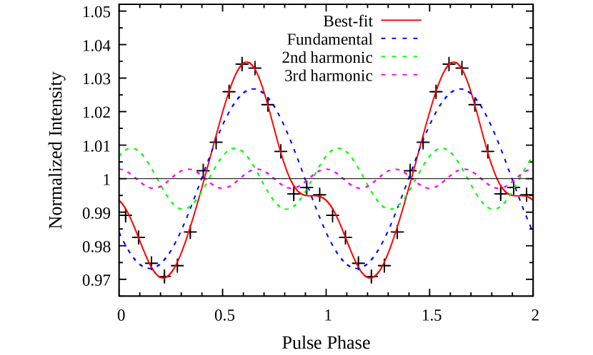
Figure 5: The average pulse profile (black points) of SAX J1808.4-3658 obtained epoch-folding the AstroSat/LAXPC data with $\bar{\nu}$ in the energy range 3–20 keV after correcting for the orbital solution. The epoch used was $T_{0}=58709.74$ MJD. The best-fitting model (red solid line) is the superposition of three sinusoidal functions with harmonically related periods. The fundamental, second and third harmonic components are presented by the blue, green and magenta dashed lines, respectively. For clarity, we show two cycles of the pulse profile.

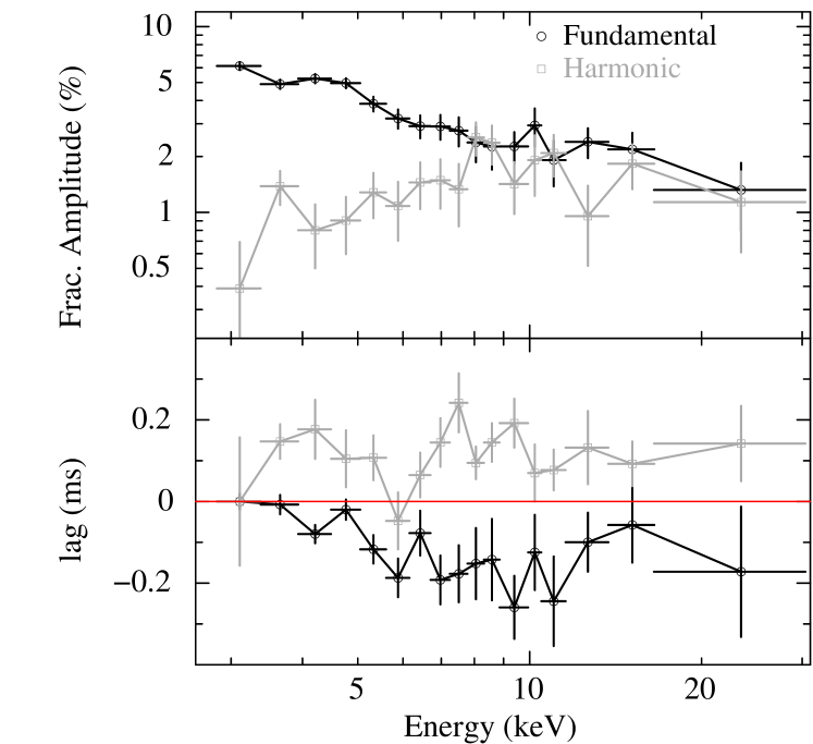
Figure 6: Top panel: The energy dependence of pulse fractional amplitude for the fundamental and harmonic. Bottom panel: The observed time lag of the fundamental and harmonic component of the pulse with energy. The zero lag corresponds to the phase of the pulse profile in 2.83–3.38 keV (channel no. 5 of LAXPC20 corresponding to 3 keV).

We also checked for the energy dependence of the pulse amplitude and phase. We divided the whole dataset depending on the different energy range and epoch-folded each with $\bar{\nu}$. Some of the energy-resolved pulse profiles are presented in fig. 8. Each folded pulse profile was then fitted with two harmonically related sinusoidal functions (third harmonic was not detected in energy-resolved pulse profiles, likely due to poor statistics of selected intervals). Fig. 6 (top panel) shows the variation of background-corrected fractional amplitude of the fundamental (black points) and harmonic (grey points) components of the pulse. The fractional amplitude of the fundamental was found to be $\sim 5$% in 3–5 keV energy range and above 5 keV a constant decrease was observed with energy. While the harmonic component increased with energy. Fig. 6 (bottom panel) shows the time lag (calculated from the phase lag) of the fundamental and harmonic component of pulse with energy. The zero lag value corresponds to the phase of pulse profile in the energy band of $2.83-3.38$ keV. It shows negative time lag (i.e. high-energy emission is coming earlier than the softer emission) of 0.1–0.2 ms for fundamental component at higher energies (above 5 keV) while, the harmonic component shows the positive lag of similar order. By comparing top and bottom plots of Fig. 6, the phase lags seems to become specular as soon as the fractional amplitude of the two components reaches similar values (above $\sim 7$ keV).

Table 3: Timing solution of SAX J1808.4-3658 during the outburst of 2019. Errors are at $1\sigma$ confidence level.

Parameter	Case 1	Case 2
Spin Frequency, $\nu$ (Hz)	400.97521014(21)	400.97521004(26)
Spin Frequency derivative, $\dot{\nu}$ (Hz/s)	$1.1(1.7)\times 10^{-11}$	$1.8(1.9)\times 10^{-11}$
Ascending node passage, $T^{\star}$ (MJD)	58715.0221031a	58715.02212 (7)
Orbital period, $P_{\rm orb}$ (s)	7249.1552a	7249.16 (10)
Projected semi-major axis, $a_{x}\sin i/c$ (lt-ms)	62.8091a	62.83 (3)
Eccentricity, $e$	$0^{a}$
Reference epoch, $T_{0}$ (MJD)	58709.74
$\chi^{2}$/d.o.f.	46/31	41/28
ataken from (Bult et al., 2020)   .

Table 4: The best-fit spectral parameters obtained from the SXT+LAXPC spectrum of SAX J1808.4-3658. Reported errors and limits are at 90% confidence level for single parameter.

Model	Parameters	SXT+LAXPC
TBabs	$N_{H}$ ($10^{22}$ cm-2)	$0.056\pm 0.007$
DiskBB	$kT_{\rm in}$ (keV)	$1.08^{+0.03}_{-0.02}$
	Norm	$7.8^{+1.2}_{-1.0}$
NTHcomp	$\Gamma$	$1.67^{+0.02}_{-0.01}$
	$kT_{\rm seed}$ (keV)	$0.322\pm 0.025$
	inp_type	0
	$kT_{e}$ (keV)	$100^{\rm fixed}$
	Norm ($10^{-2}$)	$3.7\pm 0.3$
Gaussian 1	$E_{\rm Line}$ (keV)	$7.0^{\rm pegged}_{-0.25}$
	$\sigma$ (keV)	$1.0^{\rm pegged}_{-0.2}$
	Eqw (keV)	$0.26^{+0.11}_{-0.14}$
	Norm ($10^{-4}$)	$7\pm 2$
Gaussian 2	$E_{\rm Line}$ (keV)	$0.86^{+0.04}_{-0.07}$
	$\sigma$ (keV)	$0.08^{+0.05}_{-0.03}$
	Eqw (keV)	$0.022\pm 0.010$
	Norm ($10^{-3}$)	$2.0^{+1.4}_{-0.8}$
Constant	$C_{\rm LAXPC}$	1 (fixed)
	$C_{\rm SXT}$	$1.04\pm 0.02$
SXT Gain	Gain (eV)	$34^{+2}_{-4}$
Unabs. Flux∗	$F_{0.1-100~{}\rm keV}$	$1.3\times 10^{-9}$
Luminosity†	$L_{X}$ (erg s-1)	$1.9\times 10^{36}$
	$\chi^{2}/{\rm dof}$	700/576
∗ 0.1–100 keV Unabsorbed flux in units of erg cm-2 s-1.
†X-ray Luminosity in 0.1–100 keV for a distance of 3.5 kpc.

3.4 Broadband Spectral Analysis

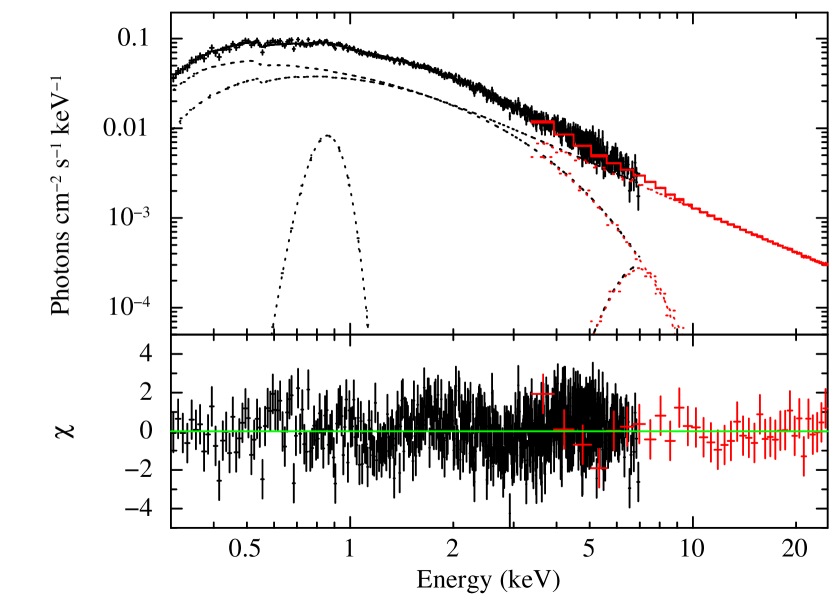
Figure 7: Broadband spectrum of SAX J1808.4-3658 from SXT and LAXPC instrument fitted simultaneously with best fit model tbabs*(diskbb+nthcomp+gaussian+gaussian). Panel below show residuals ($\chi$=(data-model)/error) with respect to best fit model.

We modelled the SXT (0.3–7 keV) and LAXPC (3–25 keV) spectrum simultaneously. Both spectra were grouped using grppha to have a minimum count of 20 counts per bin. An inter-instrumental calibration constant was added, which was fixed to 1 for LAXPC and allowed to vary for SXT. We also allowed the gain of response matrix for SXT to vary, with slope fixed at 1. A gain offset of $\sim 34$ eV was obtained. A systematic uncertainty of 2% was also introduced during the spectral fitting (Antia et al., 2017; Sharma et al., 2020). We used xspec (Arnaud, 1996) for the spectral fitting with the component tbabs to model interstellar neutral hydrogen absorption (Wilms et al., 2000).

To model the broadband spectrum, we first started with the absorbed thermal Comptonized emission model, nthcomp (Zdziarski et al., 1996; Życki et al., 1999). The nthcomp model pictures that the hot electrons Compton up-scatter the seed photons originating from the NS surface/boundary layer or inner accretion disc. Using parameter inp_type, input seed type can be selected. During all fitting, the electron temperature was unconstrained so we fixed it at reasonable value of 100 keV. The obtained fit with tbabs$\times$nthcomp was unacceptable with either of input seed photon types ($\chi^{2}/{\rm dof}\sim 1133/583$).

We then added a thermal component in form of a single temperature blackbody. It did not provide a satisfactory fit ($\chi^{2}/{\rm dof}=826/581$). We then replaced single temperature blackbody with multi-coloured blackbody (diskbb; Mitsuda et al., 1984) as the thermal component and set blackbody as seed (inp_type = 0). It provided slight improvement with $\chi^{2}/{\rm dof}=758/581$. The fit showed systematic residuals around 7 keV which hints at the Fe emission line (e.g., Cackett et al., 2009; Papitto et al., 2009; Di Salvo et al., 2019), so we added a Gaussian component to the model. During the fit, we constrained the emission line energy to be within 6.4–7.0 keV energy range (corresponds to Fe K emission). We found that the Gaussian line energy pegged at upper limit of 7 keV with width broader than $1$ keV. So we constrained the Gaussian line width to be within 0 to 1 keV. Addition of this Gaussian component improved the fit significantly to $\chi^{2}/{\rm dof}\sim 726.7/579$ with F-test probability of improvement by chance $\sim 5\times 10^{-6}$. The equivalent width of this iron emission line feature was about $\sim 0.26$ keV, while $\sim 0.1$ keV was observed with the NuSTAR observation of 2015 outburst (Di Salvo et al., 2019). Further, the obtained spectral residuals at low energies hints at some emission feature around 0.9 keV, possibly due to Ne ix or Fe L blend. Similar emission features have been seen with XMM-Newton observation (Di Salvo et al., 2019). This encouraged us to add another Gaussian emission line model. Addition of emission line at $\sim 0.85$ keV further improved the fit to $\chi^{2}/{\rm dof}\sim 700/576$ with F-test probability of improvement by chance $\sim 9\times 10^{-5}$. The best fit 0.5–25 keV persistent spectrum of SAX J1808.4-3658 is shown in Fig. 7 and the best fit parameters are listed in Table 4. We also estimated the 0.1–100 keV unabsorbed flux of $1.3\times 10^{-9}$ erg cm^-2 s^-1 from the best fit model which translate to X-ray luminosity of $1.9\times 10^{36}$ erg s^-1 for a distance of 3.5 kpc (Galloway & Cumming, 2006). We also tried to change the input seed source to disc and we obtained similar spectral fit parameters except $kT_{\rm seed}=0.57$ keV with $\Delta\chi^{2}=+6$ for no additional dof.

4 Discussion and Conclusion

SAX J1808.4-3658 was observed in its ninth outburst in 2019. The AstroSat observed it for $\sim 1.5$ days near the peak of the outburst. We report results from our broadband timing and spectral study of SAX J1808.4-3658 performed using AstroSat data. The 0.004–200 Hz PDS showed noise components which can be described by three Lorentzian functions with integrated rms of 17.5%, 11% and 13%. Moreover, we found coherent X-ray pulsations at $\sim 401$ Hz. Pulse timing results obtained are compatible within the errors with the solution obtained with NICER (Bult et al., 2020). The pulse profiles obtained in the energy bands 3–20 keV suggest a fractional amplitude of 3.5%, 1.2% and 0.37% for fundamental, second and third harmonic, respectively. Using pulse phase delays, we obtained an upper limits ($3\sigma$) on the spin down rate of $\sim-4\times 10^{-11}$ Hz s^-1 and spin up rate of $\sim 7\times 10^{-11}$ Hz s^-1 for the AstroSat observation duration.

We also checked for the dependence of fractional amplitude and phase lag on the energy in the 3–30 keV range. The fractional amplitude and phase lag were found to be energy dependent as previously observed (e.g., Hartman et al., 2009; Sanna et al., 2017; Bult et al., 2020). The fundamental component showed fractional amplitude of $\sim 5\%$ up to 5 keV, after that it starts decreasing and reached around 2%. While the harmonic component showed an increasing trend in 3–30 keV energy range from $\sim 1\%$ to 2%. Similar trend of increase in the fractional amplitude of the harmonic with energy has been observed in previous outbursts. The energy dependence of the fractional amplitudes varies considerably between different outbursts (e.g., Hartman et al., 2009; Patruno et al., 2009a; Sanna et al., 2017). Also, we did not detect any drop in fractional amplitude in 6–7 keV energy range (correspondence to the Fe line) as observed in the 2008 and 2015 outburst (Patruno et al., 2009a; Sanna et al., 2017).

SAX J1808.4-3658 is known to show energy dependent time lags in which soft X-rays lag hard X-rays, i.e. the pulse peaks at a later phase in softer energies (e.g., Cui et al., 1998; Gierliński et al., 2002; Hartman et al., 2009; Ibragimov & Poutanen, 2009). We also found similar trend with LAXPC. The lags for fundamental component is soft and increased from 3 to $\sim 10$ keV. While the harmonic component showed opposite trend, i.e. hard lags of similar order. The lags of SAX J1808.4-3658 are flux dependent and increases with drop in accretion rate. The soft lags in the fundamental observed throughout the outbursts while lags for harmonic are less pronounced or becomes hard lags when source flux is high (Hartman et al., 2009; Ibragimov & Poutanen, 2009). These lags can be explained by the model where the soft thermal component and Comptonization emissivity (or beaming) patterns are different, which is affected in a different way by the fast stellar rotation (Gierliński et al., 2002; Poutanen & Gierliński, 2003; Ibragimov & Poutanen, 2009).

The 0.3–25 keV broadband spectrum of SAX J1808.4-3658 was well described by the combination of a thermal component as multi-coloured blackbody, Comptonized emission of soft thermal photons and emission lines. A multi-coloured disc-like component statistically better fits the soft continuum than a single temperature blackbody. The thermal emission was found to be of $\sim 1$ keV temperature with compact emission size, possibly from NS or accretion column. The Comptonized emission associated to a hot corona is characterized by a photon index of $1.67$. A power-law photon index of 1.89 was measured from NuSTAR observation of 2019 at the outburst peak (Sanna et al., 2019). The electron temperature of corona was unconstrained and input seed temperature was found to be $\sim 0.3$ keV for blackbody seed and $\sim 0.5$ keV for diskbb seed. This soft component provides the seed photons to the Comptonized medium which is not directly visible. The best-fitting spectral parameters suggest that the source was in the hard spectral state during the AstroSat observation (Table 4). Throughout the outburst, the X-ray spectrum was hard during both the main outburst peak and the reflaring period (Bult et al., 2019b, c; Sanna et al., 2019). The hardness ratio observed from AstroSat did not show any significant variations, suggesting source to be in the same state throughout the observation duration. Also, no significant variations in the hardness ratio was observed with Swift/XRT during the whole outburst of 2019 (Baglio et al., 2020). Therefore, SAX J1808.4-3658 never left the hard state and went directly from a hard-state main outburst to the reflaring state (see e.g. Patruno et al., 2016; Baglio et al., 2020). During the outburst of 2015, Di Salvo et al. (2019) reported the state transition in SAX J1808.4-3658 with XMM-Newton (soft state) and NuSTAR (hard state) observations.

Generally, AMXPs show the hard spectrum with electron temperature of few tens of keV (Falanga et al., 2005; Gierliński & Poutanen, 2005; Papitto et al., 2010, 2013; Wilkinson et al., 2011; Sanna et al., 2018a, b; Di Salvo et al., 2019). Another AMXP SAX J1748.9-2021 also showed the spectral state transition from hard to soft state during bright outbursts (Patruno et al., 2009b; Pintore et al., 2016; Li et al., 2018; Sharma et al., 2019; Sharma et al., 2020). However, during the fainter outburst where SAX J1748.9-2021 have similar luminosities as of SAX J1808.4-3658 ($\sim 10^{36}-10^{37}$ erg s^-1), source seems to stay in the hard state and do not show state transitions (in ’t Zand et al., 1999; Sharma et al., 2020). So AMXPs show hard spectrum like faint transients when emitting at low luminosities.

Data Availability

Data used in this work can be accessed through the Indian Space Science Data Center (ISSDC) at https://astrobrowse.issdc.gov.in/astro_archive/archive/Home.jsp.

Appendix A Energy-resolved pulse profiles

Figure 8: Energy-resolved pulse profiles of SAX J1808.4-3658. The energy range used is mentioned in respective panels.

References

- Agrawal (2006) Agrawal P. C., 2006, Advances in Space Research, 38, 2989
- Ambrosino et al. (2021) Ambrosino F., et al., 2021, Nature Astronomy, 5, 552
- Antia et al. (2017) Antia H. M., et al., 2017, ApJS, 231, 10
- Arnaud (1996) Arnaud K. A., 1996, in Jacoby G. H., Barnes J., eds, Astronomical Society of the Pacific Conference Series Vol. 101, Astronomical Data Analysis Software and Systems V. p. 17
- Baglio et al. (2019a) Baglio M. C., Russell D. M., Lewis F., 2019a, The Astronomer’s Telegram, 13103, 1
- Baglio et al. (2019b) Baglio M. C., Russell D. M., Lewis F., Saikia P., 2019b, The Astronomer’s Telegram, 13162, 1
- Baglio et al. (2020) Baglio M. C., et al., 2020, ApJ, 905, 87
- Belloni et al. (2002) Belloni T., Psaltis D., van der Klis M., 2002, ApJ, 572, 392
- Bhattacharyya & Strohmayer (2007) Bhattacharyya S., Strohmayer T. E., 2007, ApJ, 656, 414
- Bult & van der Klis (2015) Bult P., van der Klis M., 2015, ApJ, 806, 90
- Bult et al. (2019a) Bult P., et al., 2019a, ApJ, 885, L1
- Bult et al. (2019b) Bult P. M., et al., 2019b, The Astronomer’s Telegram, 13001, 1
- Bult et al. (2019c) Bult P. M., Gendreau K. C., Arzoumanian Z., Strohmayer T. E., Chakrabarty D., Jaisawal G. K., Chenevez J., Guver S. G. T., 2019c, The Astronomer’s Telegram, 13077, 1
- Bult et al. (2020) Bult P., Chakrabarty D., Arzoumanian Z., Gendreau K. C., Guillot S., Malacaria C., Ray P. S., Strohmayer T. E., 2020, ApJ, 898, 38
- Bult et al. (2022) Bult P., et al., 2022, arXiv e-prints, p. arXiv:2208.04721
- Burderi et al. (2007) Burderi L., et al., 2007, ApJ, 657, 961
- Burderi et al. (2009) Burderi L., Riggio A., di Salvo T., Papitto A., Menna M. T., D’Aì A., Iaria R., 2009, A&A, 496, L17
- Cackett et al. (2009) Cackett E. M., Altamirano D., Patruno A., Miller J. M., Reynolds M., Linares M., Wijnands R., 2009, ApJ, 694, L21
- Cackett et al. (2010) Cackett E. M., et al., 2010, ApJ, 720, 205
- Campana & Di Salvo (2018) Campana S., Di Salvo T., 2018, in Rezzolla L., Pizzochero P., Jones D. I., Rea N., Vidaña I., eds, Astrophysics and Space Science Library Vol. 457, Astrophysics and Space Science Library. p. 149 (arXiv:1804.03422), doi:10.1007/978-3-319-97616-7_4
- Chakrabarty & Morgan (1998) Chakrabarty D., Morgan E. H., 1998, Nature, 394, 346
- Charles (2011) Charles P., 2011, in Schmidtobreick L., Schreiber M. R., Tappert C., eds, Astronomical Society of the Pacific Conference Series Vol. 447, Evolution of Compact Binaries. p. 19
- Cornelisse et al. (2009) Cornelisse R., et al., 2009, A&A, 495, L1
- Cui et al. (1998) Cui W., Morgan E. H., Titarchuk L. G., 1998, ApJ, 504, L27
- Deeter et al. (1981) Deeter J. E., Boynton P. E., Pravdo S. H., 1981, ApJ, 247, 1003
- Di Salvo & Sanna (2020) Di Salvo T., Sanna A., 2020, arXiv e-prints, p. arXiv:2010.09005
- Di Salvo et al. (2019) Di Salvo T., Sanna A., Burderi L., Papitto A., Iaria R., Gambino A. F., Riggio A., 2019, MNRAS, 483, 767
- Falanga et al. (2005) Falanga M., et al., 2005, A&A, 444, 15
- Gaensler et al. (1999) Gaensler B. M., Stappers B. W., Getts T. J., 1999, ApJ, 522, L117
- Galloway & Cumming (2006) Galloway D. K., Cumming A., 2006, ApJ, 652, 559
- Gendreau & Arzoumanian (2017) Gendreau K., Arzoumanian Z., 2017, Nature Astronomy, 1, 895
- Gierliński & Poutanen (2005) Gierliński M., Poutanen J., 2005, MNRAS, 359, 1261
- Gierliński et al. (2002) Gierliński M., Done C., Barret D., 2002, MNRAS, 331, 141
- Goodwin et al. (2019) Goodwin A. J., Russell D. M., Galloway D. K., in’t Zand J. J. M., Heinke C., Lewis F., Baglio M. C., 2019, The Astronomer’s Telegram, 12993, 1
- Goodwin et al. (2020) Goodwin A. J., et al., 2020, MNRAS, 498, 3429
- Hartman et al. (2008) Hartman J. M., et al., 2008, ApJ, 675, 1468
- Hartman et al. (2009) Hartman J. M., Patruno A., Chakrabarty D., Markwardt C. B., Morgan E. H., van der Klis M., Wijnands R., 2009, ApJ, 702, 1673
- Hasinger & van der Klis (1989) Hasinger G., van der Klis M., 1989, A&A, 225, 79
- Heinke et al. (2009) Heinke C. O., Jonker P. G., Wijnands R., Deloye C. J., Taam R. E., 2009, ApJ, 691, 1035
- Ibragimov & Poutanen (2009) Ibragimov A., Poutanen J., 2009, MNRAS, 400, 492
- in ’t Zand et al. (1998) in ’t Zand J. J. M., Heise J., Muller J. M., Bazzano A., Cocchi M., Natalucci L., Ubertini P., 1998, A&A, 331, L25
- in ’t Zand et al. (1999) in ’t Zand J. J. M., et al., 1999, A&A, 345, 100
- Jain et al. (2007) Jain C., Dutta A., Paul B., 2007, Journal of Astrophysics and Astronomy, 28, 197
- Li et al. (2018) Li Z., et al., 2018, A&A, 620, A114
- Ludlam et al. (2017) Ludlam R. M., Miller J. M., Degenaar N., Sanna A., Cackett E. M., Altamirano D., King A. L., 2017, ApJ, 847, 135
- Mitsuda et al. (1984) Mitsuda K., et al., 1984, PASJ, 36, 741
- Mukherjee et al. (2015) Mukherjee D., Bult P., van der Klis M., Bhattacharya D., 2015, MNRAS, 452, 3994
- Ng et al. (2021) Ng M., et al., 2021, ApJ, 908, L15
- Nowak (2000) Nowak M. A., 2000, MNRAS, 318, 361
- Pan et al. (2018) Pan Y. Y., Zhang C. M., Song L. M., Wang N., Li D., Yang Y. Y., 2018, MNRAS, 480, 692
- Papitto et al. (2009) Papitto A., Di Salvo T., D’Aì A., Iaria R., Burderi L., Riggio A., Menna M. T., Robba N. R., 2009, A&A, 493, L39
- Papitto et al. (2010) Papitto A., Riggio A., di Salvo T., Burderi L., D’Aì A., Iaria R., Bozzo E., Menna M. T., 2010, MNRAS, 407, 2575
- Papitto et al. (2013) Papitto A., et al., 2013, MNRAS, 429, 3411
- Parikh & Wijnands (2019) Parikh A. S., Wijnands R., 2019, The Astronomer’s Telegram, 13000, 1
- Patruno & Watts (2012) Patruno A., Watts A. L., 2012, preprint, (arXiv:1206.2727)
- Patruno et al. (2009a) Patruno A., Rea N., Altamirano D., Linares M., Wijnands R., van der Klis M., 2009a, MNRAS, 396, L51
- Patruno et al. (2009b) Patruno A., Altamirano D., Hessels J. W. T., Casella P., Wijnands R., van der Klis M., 2009b, ApJ, 690, 1856
- Patruno et al. (2009c) Patruno A., Watts A., Klein Wolt M., Wijnands R., van der Klis M., 2009c, ApJ, 707, 1296
- Patruno et al. (2016) Patruno A., Maitra D., Curran P. A., D’Angelo C., Fridriksson J. K., Russell D. M., Middleton M., Wijnands R., 2016, ApJ, 817, 100
- Patruno et al. (2017) Patruno A., et al., 2017, ApJ, 841, 98
- Pintore et al. (2016) Pintore F., et al., 2016, MNRAS, 457, 2988
- Poutanen & Gierliński (2003) Poutanen J., Gierliński M., 2003, MNRAS, 343, 1301
- Russell et al. (2019) Russell D. M., Goodwin A. J., Galloway D. K., in’t Zand J. J. M., Lewis F., Baglio M. C., 2019, The Astronomer’s Telegram, 12964, 1
- Sanna et al. (2017) Sanna A., et al., 2017, MNRAS, 471, 463
- Sanna et al. (2018a) Sanna A., et al., 2018a, MNRAS, 481, 1658
- Sanna et al. (2018b) Sanna A., et al., 2018b, A&A, 610, L2
- Sanna et al. (2019) Sanna A., Di Salvo T., Burderi L., Riggio A., Gambino A., Iaria R., 2019, The Astronomer’s Telegram, 13022, 1
- Sanna et al. (2020) Sanna A., et al., 2020, MNRAS, 495, 1641
- Sanna et al. (2022a) Sanna A., et al., 2022a, MNRAS, 514, 4385
- Sanna et al. (2022b) Sanna A., et al., 2022b, MNRAS, 516, L76
- Sanna et al. (2022c) Sanna A., et al., 2022c, The Astronomer’s Telegram, 15559, 1
- Sharma et al. (2019) Sharma R., Jain C., Dutta A., 2019, MNRAS, 482, 1634
- Sharma et al. (2020) Sharma R., Beri A., Sanna A., Dutta A., 2020, MNRAS, 492, 4361
- Sharma et al. (2022) Sharma R., Jain C., Rikame K., Paul B., 2022, MNRAS,
- Singh et al. (2014) Singh K. P., et al., 2014, in Space Telescopes and Instrumentation 2014: Ultraviolet to Gamma Ray. p. 91441S, doi:10.1117/12.2062667
- Singh et al. (2016) Singh K. P., et al., 2016, in den Herder J.-W. A., Takahashi T., Bautz M., eds, Society of Photo-Optical Instrumentation Engineers (SPIE) Conference Series Vol. 9905, Space Telescopes and Instrumentation 2016: Ultraviolet to Gamma Ray. p. 99051E, doi:10.1117/12.2235309
- Singh et al. (2017) Singh K. P., et al., 2017, Journal of Astrophysics and Astronomy, 38, 29
- Tudor et al. (2017) Tudor V., et al., 2017, MNRAS, 470, 324
- van der Klis (2004) van der Klis M., 2004, arXiv e-prints, pp astro–ph/0410551
- van Straaten et al. (2005) van Straaten S., van der Klis M., Wijnands R., 2005, ApJ, 619, 455
- Wang et al. (2001) Wang Z., et al., 2001, ApJ, 563, L61
- Wang et al. (2013) Wang Z., Breton R. P., Heinke C. O., Deloye C. J., Zhong J., 2013, ApJ, 765, 151
- Wijnands & van der Klis (1998a) Wijnands R., van der Klis M., 1998a, Nature, 394, 344
- Wijnands & van der Klis (1998b) Wijnands R., van der Klis M., 1998b, ApJ, 507, L63
- Wijnands et al. (2003) Wijnands R., van der Klis M., Homan J., Chakrabarty D., Markwardt C. B., Morgan E. H., 2003, Nature, 424, 44
- Wilkinson et al. (2011) Wilkinson T., Patruno A., Watts A., Uttley P., 2011, MNRAS, 410, 1513
- Wilms et al. (2000) Wilms J., Allen A., McCray R., 2000, ApJ, 542, 914
- Yadav et al. (2016) Yadav J. S., et al., 2016, in Space Telescopes and Instrumentation 2016: Ultraviolet to Gamma Ray. p. 99051D, doi:10.1117/12.2231857
- Zdziarski et al. (1996) Zdziarski A. A., Johnson W. N., Magdziarz P., 1996, MNRAS, 283, 193
- Życki et al. (1999) Życki P. T., Done C., Smith D. A., 1999, MNRAS, 309, 561