Constructing Organism Networks from Collaborative Self-Replicators

Abstract

We introduce organism networks, which function like a single neural network but are composed of several neural particle networks; while each particle network fulfils the role of a single weight application within the organism network, it is also trained to self-replicate its own weights. As organism networks feature vastly more parameters than simpler architectures, we perform our initial experiments on an arithmetic task as well as on simplified MNIST-dataset classification as a collective. We observe that individual particle networks tend to specialise in either of the tasks and that the ones fully specialised in the secondary task may be dropped from the network without hindering the computational accuracy of the primary task. This leads to the discovery of a novel pruning-strategy for sparse neural networks.

I Introduction

Self-replication (SR) has always been regarded one of the central aspects of life [1]. Recent literature has shown spiking interest in enabling neural networks (NNs) to self-replicate (cf. [2, 3, 4]), mostly for the pure reason of creating more lifelike entities from neural networks, which are currently the most prominent tools to encode complex behaviour in a way that is easily accessible to machine learning. Eventually, one may hope to lift some limitations imposed by current neural network architectures via means of self-replication (SR) to decrease volatility in the training process or to create new means of information interchange between such networks.

Instances of self-replicating neural networks have already been given additional tasks that are more directly useful to the system’s designer than pure SR — a kind of ultimate purpose (cf. [2, 5, 4]). However, in all of these instances, an SRNN is expected to perform said task on its own or only with indirect support from other networks during training [5]. Furthermore, the tasks visited by Gabor et al. [5] can be described as very basic arithmetic operations.

Therefore, in this study, we built upon the work by Gabor et al. [5] in establishing singular self-replicating neural networks as members of a group of many networks that collaborate on learning to solve a joint auxilary task (AT). Effectively, we define a structure we call an organism network (ON), which looks like any other neural network from the outside but on the inside is composed of various other NNs we call particle networks (PNs). While each individual of these particle networks is trained to self-replicate, the whole ON is trained to perform a ‘meaningful’ (auxiliary) task (like the simple addition of numbers or the classification of images). Thus, we push the metaphor of self-replicating NNs one step further by having them behave in an (at least more) similar way to cells in multicellular biological specimen.

As the parameter space of the complete organism network with all its PNs grows to large dimensions, we consider showing the feasibility of training such a structure to meaningful and useful behaviour as one main contribution of this paper, even though organism networks cannot quite compete with standard approaches for training efficiency on their collaborative auxilary task yet. Most interestingly, we observe that, with a simpler problem like float addition, all PNs can be trained to be self-replicators while performing the AT; a more complicated task like classification of images in the MNIST-dataset (MNIST), however, gives rise to fully autonomous specialisation within the PNs. This means that certain PNs tend to focus on SR while others focus on the auxilary task. Our experiments suggest that, when pruning these PNs from a comparable sized NN, we can still retain almost all the organism network’s external function (AT). As a novel finding, we also observe better performance in comparison to a comparable network pruned by a global unstructured ‘l1-pruning’ method.

The structure is as follows: We present a brief recap of relevant background in the field of self-replicating neural network in Section II, before proposing the concept and architecture of organism networks in Section III. Experiments with two different auxilary tasks of increasing difficulty and the investigation of resulting performances can be found in Sections IV & V. Finally, we discuss related work in Section VI and conclude our findings in Section VII.

II Self-Replicating Networks

We follow Gabor et al. [3] in the definition of self-replicating neural networks, of which we sum up shortly all relevant and adopted material. We will also briefly define our approach and notation for the underlying neural network basics.

Definition 1 (neural network)

A neural network is a function $\mathcal{N}:\mathbb{R}^{p}\to\mathbb{R}^{q}$ with $p$ inputs and $q$ outputs. This function is defined via a graph made up of $r$ layers $L_{1},...,L_{r}$ where each layer $L_{l}$ consists of $|L_{l}|$ cells $C_{1},...,C_{|L_{l}|}$, which make up the graph’s vertices, and each cell $C_{l,c}$ of the layer $L_{l}$ is connected to all cells of the previous layer, i.e., $C_{l-1,d}$ for $d=1,...,|L_{l-1}|$, via the graph’s edges. Each edge of a cell $C_{l,c}$ is assigned an edge weight $E_{l,c,e}\in\mathbb{R},e=1,...,|L_{l-1}|$. Given a fixed graph structure, the vector of all edge weights $\mathbf{w}=\overline{\mathcal{N}}=\langle E_{l,c,e}\rangle_{l=1,...,r,c=1,...,|L_{l}|,e=1,...,|L_{l-1}|}$ defines the network’s functionality.

A network’s output given an input $\mathbf{x}\in\mathbb{R}^{p}$ is given via $\mathbf{y}=\mathcal{N}(\mathbf{x})=\langle O(r,c)\rangle_{c=1,...,|L_{r}|}\in\mathbb{R}^{q}$ where

$$O(l,c)=\begin{cases}x_{c}&\textit{ if }l=0,\\ \sum_{i=1}^{|L_{l-1}|}E_{l,c,i}\cdot O(l-1,c)&\textit{ otherwise.}\end{cases}$$

Note that Definition 1 is not the most general way to define neural networks and especially our definition of $O$ already imposes linear activation as we use it for the basic SRNNs in this paper. Further note that during all experiments, the network architecture remains fixed so that we can deduce a network’s function using only its weight vector. To better understand the internal structure of a neural network and how the function is derived from architecture and weights, please refer to Lecun et al. [6] or the definitions by Gabor et al. [3], which match our formalism.

To allow for SR on a formal level, we need to define the NN in a way so that it can process all of its own weights. As the weight vector of an arbitrary network always contains at least as many weights as its input and output dimensions combined, it is rather difficult to implement a neural network that can process all its own parameters in a single activation step. As discussed by Gabor et al. [3], it is possible to pass every weight parameter to the network one by one alongside with some meta-data regarding the weight parameter’s position within the network (w.r.t. to layer, neuron, weight), which enables the NN to process a vector as large as its own weight vector via several iterations. We adopt this so called weightwise reduction [3] for our research, which also allows for interactions between particles in future experiments.

An application of one network reduced in this way onto another network (or itself) is defined as follows:

Definition 2 (weightwise application)

Let $\mathcal{M},\mathcal{N},\mathcal{O}:\mathbb{R}^{4}\to\mathbb{R}$ be neural networks. Let the weights of $\mathcal{M}$ be $\overline{\mathcal{M}}=\langle v_{i}\rangle_{0\leq i<|\overline{\mathcal{M}}|}$. A neural network $\mathcal{O}$ is the result of weightwise application of $\mathcal{N}$ onto $\mathcal{M}$, written $\mathcal{O}=\mathcal{N}\lhd_{\textit{ww}}\mathcal{M}$, iff

$$\overline{\mathcal{O}}=\langle\mathcal{N}(v_{i},L(i),C(i),E(i))\rangle_{0\leq i<|\overline{\mathcal{M}}|}$$

where $L(i)$ is the layer of the weight $i$, $C(i)$ is the cell the weight $i$ leads into and $E(i)$ is the positional number of edge weight $i$ among the weights of its cell.

Gabor et al. [3] define SR as a network’s ability to reproduce its own weights via weightwise application on itself (weight-wise self-application). In other words, fed with a single weight value and a corresponding positional encoding, the network learns a mapping to reliably reproduce each weight. Since floating-point mathematics is imprecise in today’s computers, we expect the weights to not be reproduced exactly but only within an $\varepsilon$ distance. Once a neural network can achieve sufficiently precise self-replication (SR), it is called an $\varepsilon$-fixpoint.

Definition 3 ($\varepsilon$-fixpoint)

Given a neural network $\mathcal{N}$ with weights $\overline{\mathcal{N}}=\langle v_{i}\rangle_{0\leq i<|\overline{\mathcal{N}}|}$. Let $\varepsilon\in\mathbb{R}$ be the error margin of the fixpoint property. Let $\mathcal{N}^{\prime}=\mathcal{N}\lhd_{\textit{ww}}\mathcal{N}$ be the self-application of $\mathcal{N}$ with weights $\overline{\mathcal{N}^{\prime}}=\langle w_{i}\rangle_{0\leq i<|\overline{\mathcal{N^{\prime}}}|}$. We call $\mathcal{N}$ an $\varepsilon$-fixpoint or a fixpoint up to $\varepsilon$ iff for all $i$ it holds that $|w_{i}-v_{i}|<\varepsilon$.

In most applications of artificial intelligence, the weights for neural networks are generated via training.

Definition 4 (training)

Given a training data set $\mathbb{D}=\{(X_{i},Y_{i})\;|\;0\leq i<|\mathbb{D}|\}$ with data points consisting of an input $X_{i}$ and a desired output $Y_{i}$. We train a network $\mathcal{N}$ on $\mathbb{D}$ when we create a new network $\mathcal{N}^{\prime}$ with adjusted weights $\overline{\mathcal{N^{\prime}}}$ so to minimize the loss $\sum_{i=0}^{|\mathbb{D}|-1}|\mathcal{N^{\prime}}(X_{i})-Y_{i}|$ compared to $\mathcal{N}$. This update of weights is written as $\mathcal{N}^{\prime}=\mathcal{N}\mathrel{\reflectbox{$\leadsto$}}(X_{0},Y_{0})\mathrel{\reflectbox{$\leadsto$}}...\mathrel{\reflectbox{$\leadsto$}}(X_{|\mathbb{D}|-1},Y_{|\mathbb{D}|-1})$ or shorter $\mathcal{N}^{\prime}=\mathcal{N}\mathrel{\reflectbox{$\leadsto$}}\mathbb{D}$.

Training of Feed-Forward Neural Networks (FF NN), is usually performed via backpropagation (BP, cf. [7]). When training self-replicating NNs by BP, we can define a weightwise training operator $\mathrel{\reflectbox{$\leadsto$}}_{\textit{ww}}$ as follows:

Definition 5 (weightwise training)

Given neural networks $\mathcal{M},\mathcal{N},\mathcal{O}$ with $\overline{\mathcal{M}}=\langle v_{i}\rangle_{0\leq i<|\mathcal{M}|}$. A neural network $\mathcal{O}$ is the result of weightwise training of $\mathcal{N}$ for $\mathcal{M}$, written $\mathcal{O}=\mathcal{N}\mathrel{\reflectbox{$\leadsto$}}_{\textit{ww}}\mathcal{M}$, iff

$$\mathcal{O}=\mathcal{N}\mathrel{\reflectbox{$\leadsto$}}\{((v_{i},L(i),C(i),E(i)),v_{i})\;|\;0\leq i<|\overline{\mathcal{M}}|\}$$

where $L,C,E$ are defined as in Definition 2.

As shown by Chang and Lipson [2], subjecting a randomly initialized neural network $\mathcal{N}$ to iterated self-application, i.e., computing $\mathcal{N}\lhd_{\textit{ww}}\;\mathcal{N}\lhd_{\textit{ww}}\;...\lhd_{\textit{ww}}\;\mathcal{N}$, causes the network to converge/diverge to trivial fixpoints $\overline{\mathcal{N}}\in\{\mathbf{0},\mathbf{+\infty},\mathbf{-\infty}\}$. Gabor et al. [3] have shown that subjecting randomly initialized neural networks to self-training, i.e., computing $\mathcal{N}\mathrel{\reflectbox{$\leadsto$}}_{\textit{ww}}\mathcal{N}\mathrel{\reflectbox{$\leadsto$}}_{\textit{ww}}...\mathrel{\reflectbox{$\leadsto$}}_{\textit{ww}}\mathcal{N}\lhd_{\textit{ww}}\;\mathcal{N}$, results in these networks becoming (usually non-trivial) $\varepsilon$-fixpoints up to small $\varepsilon\leq 10^{-7}$.

II-A Revisiting Additional Goals

To formalize the auxilary task (AT), we include the findings of Gabor et al. [5] and adopt the procedure of their secondary (auxiliary) goal interface. They append auxiliary goals of the form $f:\mathbb{R}^{2}\to\mathbb{R}$ to networks for weightwise application for a combined input format of $\mathcal{N}:\mathbb{R}^{6}\to\mathbb{R}$. Since in our case, the auxiliary task will consist of multiplying one incoming scalar, we can simply omit the second auxiliary position and reuse this setting for our purpose. To reflect this change, we will update the wording of relevant auxiliary task definitions, briefly:

Definition 6 (replicative and auxiliary application)

Given neural networks $\mathcal{M},\mathcal{N},\mathcal{O}:\mathbb{R}^{5}\to\mathbb{R}$ with $\overline{\mathcal{M}}=\langle v_{i}\rangle_{0\leq i<|\mathcal{M}|}$. Neural network $\mathcal{O}$ is the result of replicative application of $\mathcal{N}$ for $\mathcal{M}$, written $\mathcal{O}=\mathcal{N}\lhd_{\textit{rep}}\mathcal{M}$, iff

$$\overline{\mathcal{O}}=\langle\mathcal{N}(v_{i},L(i),C(i),E(i),0)\rangle_{0\leq i<|\overline{\mathcal{M}}|}$$

where $L,C,E$ are defined as in Definition 2.

Given an input value $x\in\mathbb{R}$, the output value $y\in\mathbb{R}$ is the result of auxiliary application of input $x$, written $y=\mathcal{N}\bullet_{\textit{aux}}X$, iff

$$y=\mathcal{N}(0,0,0,0,x).$$

III Introducing the Organism Network

Single networks of the structure described in the last subsection have proven to learn the ability to not only fulfil the SR-property (cf. Definition 3), but also complete an auxilary task. In recent experiments, while ‘living’ in the same environment (interacting from time to time through well-defined operators in the context of an artificial chemistry system), their ‘lives’ were focused on either learning only their individual SR-function [8] or SR plus an additional auxilary task [5]. Those individual ATs, even though being the same for all SR-networks, are still only assigned to and learned by individual SRNNs and do not construct any interactions (between the individuals) or incentive to work together. In this work, we now introduce the concept to learn a shared task (AT), for which each SRNN plays its individual part. Our end-to-end trainable architecture (in which the SRNNs are embedded) is built to fulfil a global task, while enabling SRNNs to learn to self-replicate. Inspired by the concept of biological organism, we define a hierarchical structure named organism network (ON) that is built from groups (cells) of individual SRNNs. As we use a very specific interface for our implementation of the SRNN, we also refer to them as particle networks (PNs).

The requirements are as follows: (1) The structure has to work with the given PN interface so that the self-replication property can still be achieved. (2) The individual particle networks should still be able to interact with each other, hence a common task interface. (3) In addition to that, all PNs’ auxilary task functions must work within a defined structure so that the organism network as a whole can fulfil a higher purpose.

To meet these requirements, we define the PNs’ auxilary task (AT) (or goal) as the linear function of ‘multiply $x$ by a fixed value $w$’. Figure 1a depicts the PN and the described SRNN interface (grey, green). While only exposing the auxilary task input (green) by passing zero to the unused self-application (SA) inputs, we can define unions of PNs (Figure 1b) whose outputs are added up to form a single group response. These unions which compute $\sum^{0}_{i}(PN_{i}(X_{i}))$ are commonly known as cells in a neural network. In other words, we propose a structured computational graph-architecture (ON, Figure 1c) in which interconnected groups ( cell (C), Figure 1b) of individuals (PN, Figure 1a) are combined, so that each PN then behaves like a cell’s weight in an NN.

Definition 7 (organism network)

An organism network (ON) is a neural network (NN) (cf. Definition 1) whose edges are not populated by scalar weights $E_{l,c,e}$ but instead by particle networks $\mathcal{M}_{l,c,e}$ (as defined by the PNs’ weight vectors $\overline{\mathcal{M}_{l,c,e}}$), i.e., $\mathbf{w}=\overline{\mathcal{ON}}=\langle\mathcal{M}_{l,c,e}\rangle_{l=1,...,r,c=1,...,|L_{l}|,e=1,...,|L_{l-1}|}$.

A ON’s output provided an input $\mathbf{x}\in\mathbb{R}^{p}$ is given via $\mathbf{y}=\mathcal{ON}(\mathbf{x})=\langle O^{\prime}(r,c)\rangle_{c=1,...,|L_{r}|}\in\mathbb{R}^{q}$ where

$$O^{\prime}(l,c)=\begin{cases}x_{c}&\textit{ if }l=0,\\ \sum_{i=1}^{|L_{l-1}|}\mathcal{M}_{l,c,i}(0,0,0,0,O^{\prime}(l-1,c))&\textit{ otherwise.}\end{cases}$$

Given the already established research in the field of SRNNs, this architecture (ON, Figure 1) can be trained end-to-end as an arbitrary linear function approximator, while each PN still fulfils its self-replication property.

Definition 8 (goal fulfilment)

An organism network (ON) of particle networks $\mathcal{M}_{1},...,\mathcal{M}_{|\mathcal{ON}|}$ has fulfilled its goal (up to a precision of $\varepsilon,\zeta$) iff

• all particle networks $\mathcal{M}_{1},...,\mathcal{M}_{|\mathcal{ON}|}$ are $\varepsilon$-fixpoints (cf. Definition 3) and

• for all specified test data $(x,y)$ the network’s output $y^{\prime}=\mathcal{ON}(x)$ fulfils $|y-y^{\prime}|\leq\zeta$.

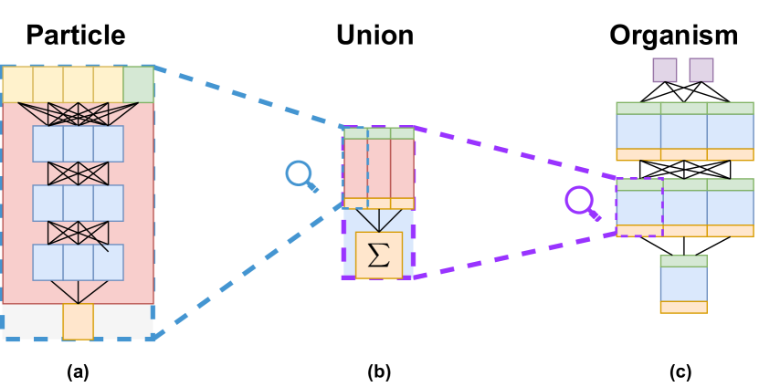
Figure 1: Schematic overview of the ON architecture. (a) A PN approximates a weight application (output y, small orange box) for a given input value (x, green box), embedded in the auxiliary task input format of Definition 6 (yellow boxes). (b) A cell aggregates many predictions of the individual PNs composing them (orange bar/vector) into one sum per union (big orange box). (cc) The full ON (here: two inputs, three hidden layers) finally invokes many cells, bundled layer-wise as is common for deep NNs.

Due to the given hierarchical order of ON, C, and PN, we call the optimization toward the collaborative auxilary tasks of PNs global — while both self-replication and ‘acting-as-a-weight’ are considered local tasks.

IV Experiment #1 — Float Addition

To provide a proof-of-concept of the PNs indeed being able to cooperate as individuals on a global auxilary task, we start with a simple task: the addition of two floating point precision numbers. This task has been shown to be learnable in conjunction with SR for a single SRNN by Gabor et al. [5]. To train towards the fulfilment of both the global AT and the local SR task, we need to alternate the training schedule between the two tasks.

Using Stochastic Gradient Descent (SGD; $lr=0.004$, $momentum=0.9$, $epochs=50$) we train each PN 25 steps of self-replication for each of the 20 batches in the primary (addition) task-dataset. Sufficient sizes for the PNs and ON (w.r.t. cells & layers; (3,3), (3,2)) were determined empirically.

IV-A Performance, Stability, and Robustness

In accordance with Gabor et al. [3, 5] we tested the particle networks (PNs) for self-replication (SR) properties and studied their convergence and stability. Figure 2 shows the timeline of all PNs within an organism network slowly acquiring the SR-capability over the course of training.

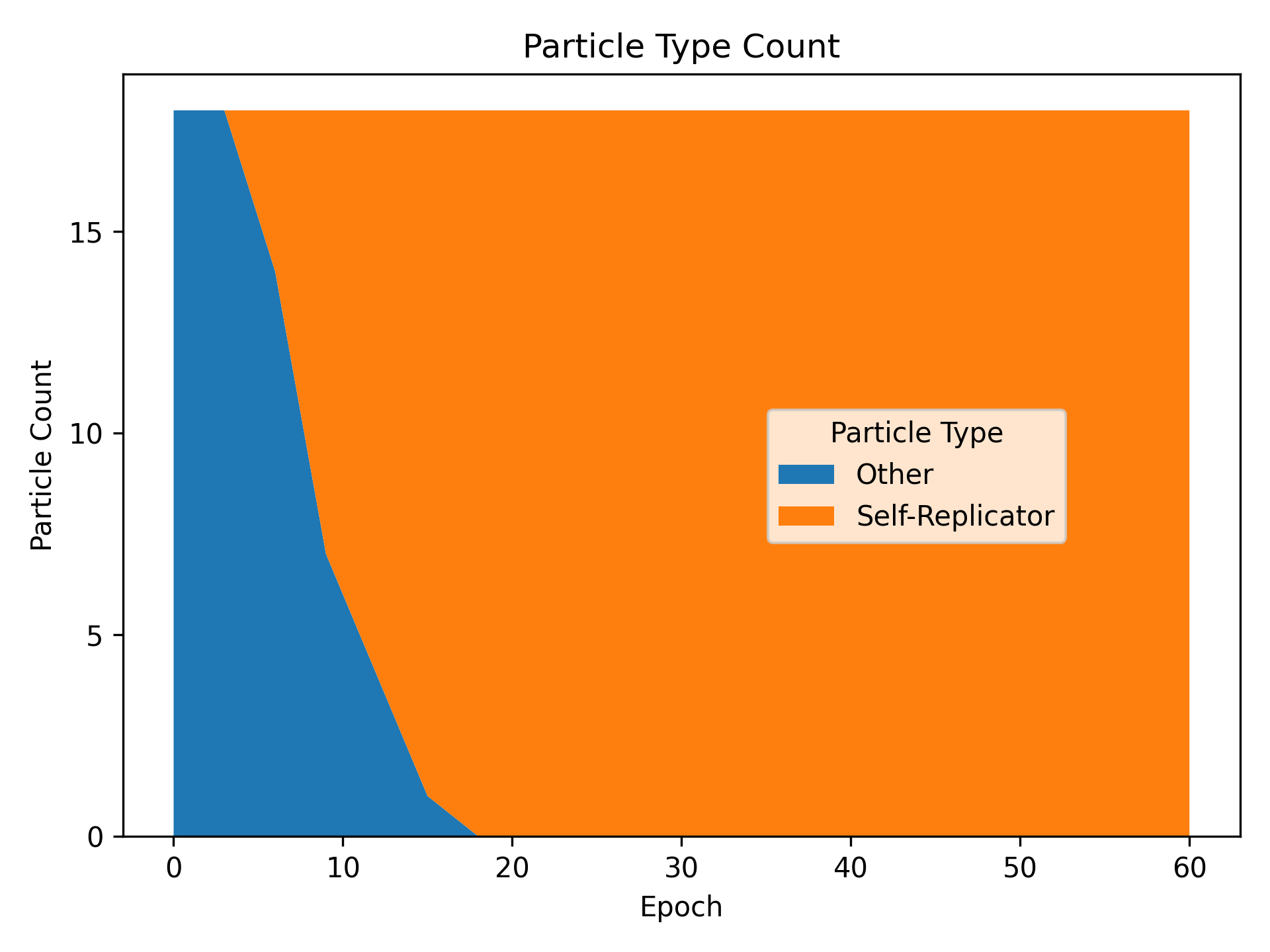
Figure 2: Distribution of PNs types ($PN_{SR}$ (orange), $PN_{F}$ (blue); Y-axis) composing the ON over the course of training experiment #1, in epochs (X-axis).

Even through the variance of several runs, we can observe both the local self-train loss and, shortly thereafter, the global addition task loss reaching their best predictions within the span of relative few epochs (cf. Figure 3). This speaks in favor of a robust and stable training behaviour, which is not surprising given the yet linear nature of the ON architecture. With both averaged losses (self-replication and auxilary task) well below the $\varepsilon$ threshold, we consider all PNs as well as the over-spanning ON as goal-networks according to Definition 8.

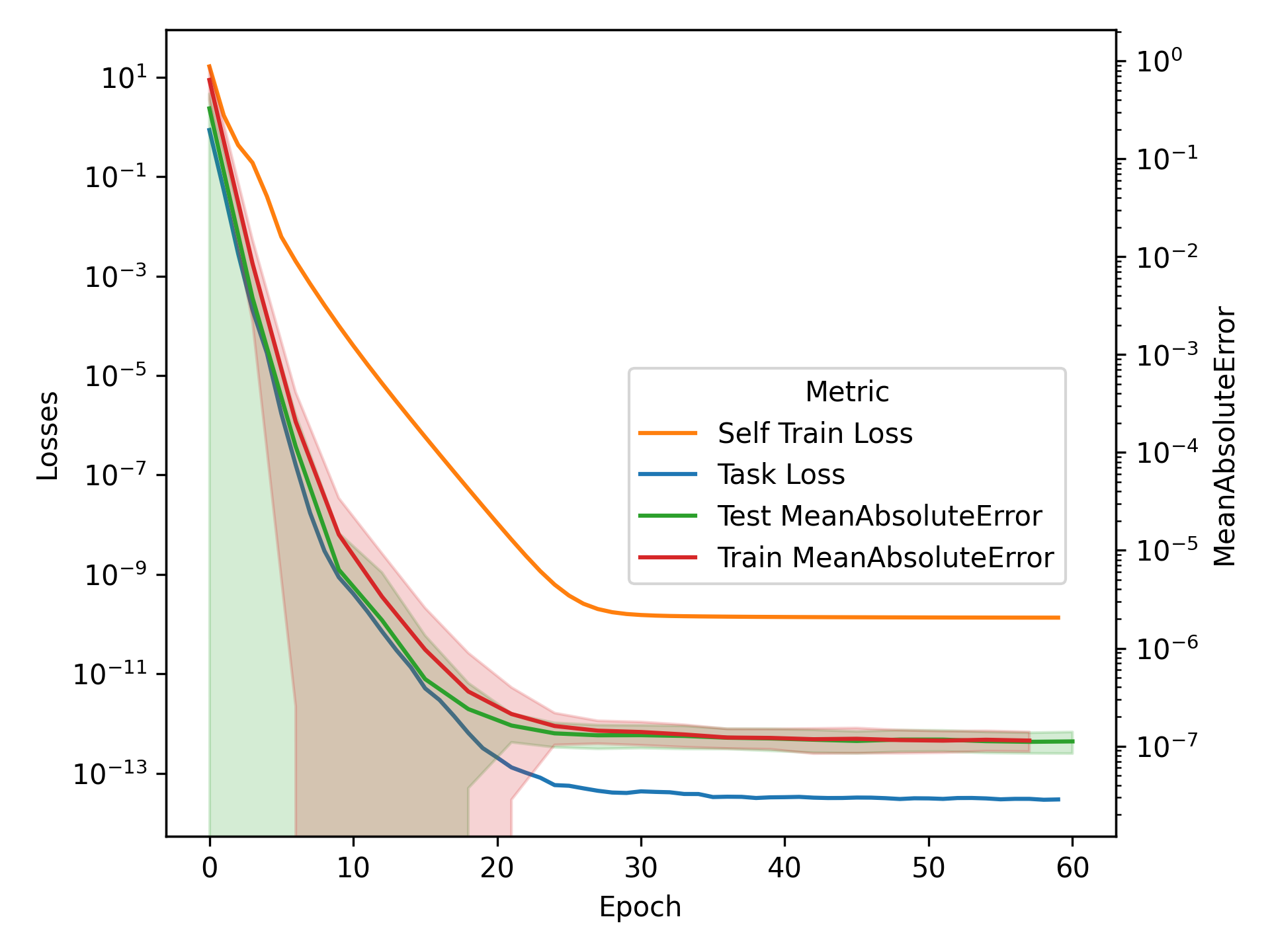
Figure 3: Mean squared error (MSE, left Y-axis) for both the local SR-task-loss (orange) and the global add-task-loss (blue), vs. the mean absolute error (MAE, right Y-axis) of the global add-task-loss, for comparison, over the course of training (red) and testing (green) ($n_{seeds}=10$, $epochs=60$, X-axis).

Regarding the robustness of the SR property, we borrow the repeated self-application experiment conducted by Gabor et al. [8] for our organism network (cf. Figure 2). We found that, in comparison to both other studies, the PNs hold their SR property for longer when applied to themselves (cf. Definition 2), some even under the influence of strong Gaussian noise ($>10^{-5}$) on the initial inputs (cf. Figure 4). Interestingly, even though the observed variance as well as the $.95$ confidence interval span over a wide margin, the average robustness per noise level is higher than shown for simple self-replicators, even perfectly constructed ones (cf. Gabor et al. [8], Figure 3). Therefore, $PN_{SR}$ seem to be even stronger $\varepsilon$-fixpoint generators than individually trained SRNNs.

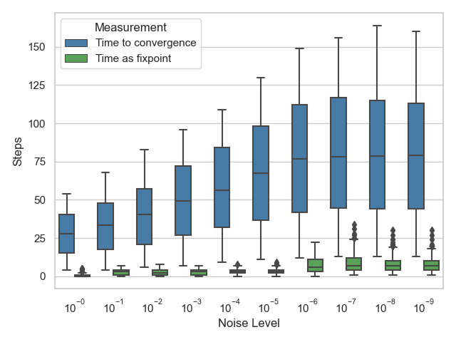
Figure 4: The robustness of PNs that did learn the SR-property $PN_{SR}$ w.r.t. the weight-wise application $\lhd_{\textit{ww}}$ (cf. Definition 2). X-axis: Range of noise applied on the initial input. Y-axis: Steps of self-application PNs keep their SR-property w.r.t. $\varepsilon=10^{-5}$ (green); steps of self-application until the network is regarded as diverged (blue).

IV-B Weight Re-Substitution

To check whether the trained particle networks (PNs) are behaving like weights in an NN, we introduce a fixed input of $x_{ON_{w}}=(0,0,0,0,1)$, matching the organism interface. The PNs’ output value, as the product of $1$ times the weight-scalar that the organism learned to represent (in a linear network), represents the extracted weight value. We then replace a conventional feed-forward NN of same size (w.r.t. number of neurons and layers) of ON parameters with the extracted weight values and calculate the absolute margin of error for the classification task. This experiment shows that our ON of approximated weight applications behaves like regular neural networks (by a margin of error of $\leq 10^{-8}$) as shown in Figure 5, but at a noticeable lower variance.

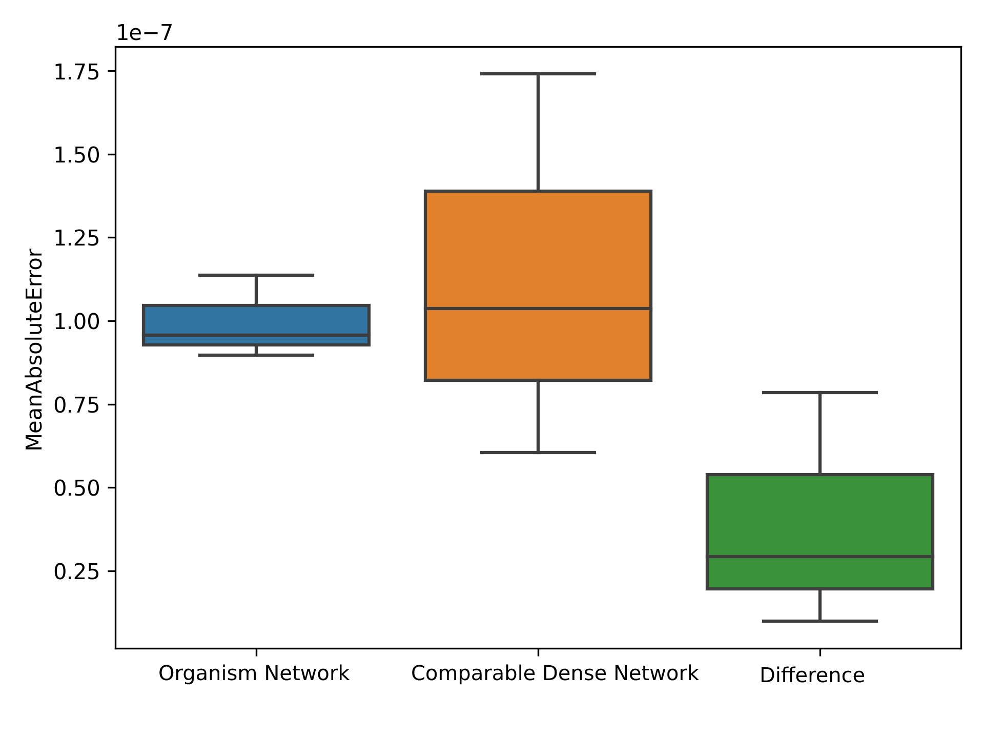
Figure 5: Absolute margin of error for the addition-task (Y-axis, scaled at 1e-7; Definition 6) after replacing parameters in a feed-forward NN of same size (w.r.t number of neurons and layers) by learned weight application of $t\in PN_{0}^{i}$ (cf. Def. 9)

V Experiment #2 — MNIST Image Classification

After confirming the basic validity of the organism network on the ‘float-addition’ task we now explore the possibility of training a bigger network with image classification as the global task. In this experiment, we intend to move the context of self-replicating organisms (and SRNNs) closer to real-world applications. As the training time and compute costs grow quickly with additional input dimensions and each additional PN, we decide in favour of a downsized variant for the scope of this research. While there may be more optimized setups in the future, we used a $(15\times 15)$ pixel variant of MNIST (cf. Deng [9]). This dataset consisting of $70,000$ images of standardized handwritten numbers ($30\times 30$px) was considered a standard deep-learning benchmark for several years. As MNIST is much harder to learn than simple addition, we prioritize the image classification task by adjusting the self-train vs. global-task-train schedule to a 5:1 ratio. To enable better organism network training, we also increase the model width and the hidden layer depth to 3 (excluding the input and output layers). Also, we introduce non-linearity in the form of the Gaussian Error Linear Unit (GELU) [10] activation function after every hidden layer. The optimizer setup remains with the same parameters.

V-A Performance, Stability, and Robustness

Figure 6 shows the losses of both tasks and the accuracies. Testing was carried out on a withheld 10,000 sample test set, as is convention (see Deng [9]). We observe the SR-loss improving much faster than expected, with the classification accuracy growing steadily to convergence. Although the results may not be state-of-the-art precision, we deem a test accuracy of $>0.8$ on an (in effect) tiny network with no bias a decent example of the ON’s capability.

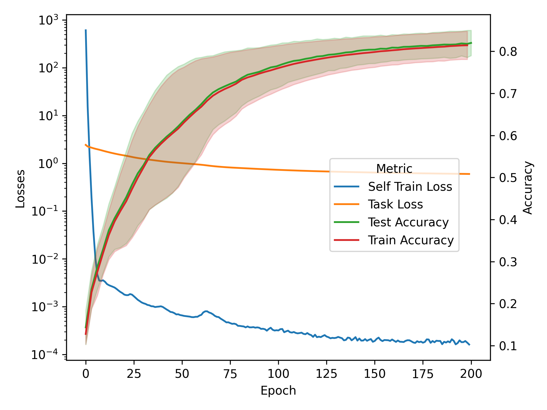
Figure 6: Losses (left X-axis) vs. accuracy (right Y-axis) for both, the local SR-task (loss blue) and the global MNIST-classification-task (loss orange) over the course of training (red) and testing (green) ($n_{seeds}=3$, $epochs=200$, X-axis).

When revisiting the test for robustness (cf. Figure 7) on PNs trained on MNIST, we observe much lower levels of robustness, which are comparable to findings in the established literature. This contrasts our previous results and leads to the assumption that, with longer training and regimes which are more focused on the SR-task, very robust and stable self-replicators are achievable.

After an in-depth hyperparameter search, we observed a major drawback: Even though the SR-loss converged fast, Figure 9 shows that just about a quarter of all PNs gained the SR-property. This contrasts with our original assumption because we had expected that all PN would achieve this property.

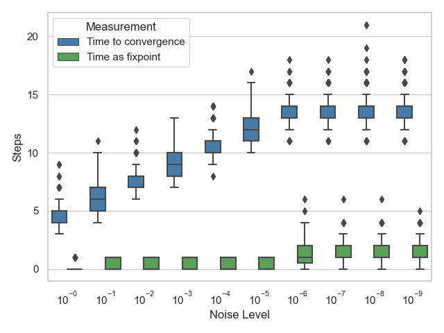
Figure 7: The robustness of PNs that did learn the SR-property $PN_{SR}$ regarding the weight-wise application $\lhd_{\textit{ww}}$ (cf. Definition 2). X-axis: Range of noise applied on the initial input. Y-axis: Steps of self-application PNs keep their SR property with $\varepsilon=10^{-5}$ (green); Steps of self-application the network was regarded as diverged (blue).

V-B Specialist Dropout Test

As it is not possible for us to train all PNs to learn both tasks at the same time, we decide to further investigate the abilities of the PNs. We assume that training on MNIST is more complex than our simple Experiment #1; PN (weights) with less importance for the auxilary task gain the SR-property $PN_{SR}$ earlier than the others $PN_{F}$. To validate our assumption, we construct a dropout test comparable to a ‘per-weight-dropout’ (i.e., making an NN sparse by pruning), in which we test the influence of both groups $[PN_{SR},PN_{F}]$ on the task accuracy (cf. Definition 9). In other words, we want to know how important a subset of weight positions is (defined by its SR-property) for solving the overall group task.

Definition 9 (dropout organism network)

Let $\mathcal{ON}$ be an organism network, so that $\overline{\mathcal{ON}}=\langle\mathcal{PN}_{i}\rangle_{i=1,...,|\overline{\mathcal{ON}}|}$ is a vector of particle networks $\mathcal{PN}_{i}:\mathbb{R}^{5}\to\mathbb{R}$ for $i=1,...,|\overline{\mathcal{ON}}|$. Let $T:(\mathbb{R}^{5}\to\mathbb{R})\to\{PN_{SR},PN_{F}\}$ be a labelling of all particle networks, with the implication that any self-replicating particle network $\mathcal{PN}$ is labelled with $T(\mathcal{PN})=\mathcal{PN}_{SR}$ and any other particle network $\mathcal{PN}$ is labelled with $T(\mathcal{PN})=PN_{F}$. Let $\mathcal{Z}:\mathbb{R}^{5}\to\mathbb{R}$ be the zero network so that $\mathcal{Z}(\_,\_,\_,\_,\_)=0$ for any input. The dropout organism network $\mathcal{ON}^{\prime}$ for $\mathcal{ON}$ w.r.t. type $t\in\{PN_{SR},PN_{F}\}$ is given via $\overline{\mathcal{ON}}=\langle D(i)\rangle_{i=1,...,|\overline{\mathcal{ON}}|}$ where $D(i)=\begin{cases}\mathcal{Z}&\textit{if }T(\mathcal{PN}_{i})=t,\\ \mathcal{PN}_{i}&\textit{otherwise.}\end{cases}$

Figure 8 depicts the accuracy after per-weight-dropout for all groups of $t\in\{PN_{SR},PN_{F}\}$ compared to the whole organism network. We observe that $PN_{SR}$-dropout results in almost no change in the measured test accuracy ($>0.001$ accuracy), which is quite surprising considering that we disable a sizable chunk of the network parameters. The other way around, $PN_{F}$-dropout disables the MNIST classification immediately. This is the expected outcome, given the vast proportion of $PN_{F}$ in the $ON$ and their connectivity (cf. Figure 11). In other words, PNs which are able to ‘specialise’ in self-replication are obviously not crucial for the group task, which allows us to reduce the networks’ parameter size by approx. $25\%$. However, we observe a slow but gradual trend towards more self-replicators ($PN_{SR}$) (cf. Figure 9), suggesting insufficient training time so that clear convergence may have simply yet to occur, which, we believe, is not as likely, given the alternating training. Instead of blindly training more epochs, we settle with this situation and analyse it further.

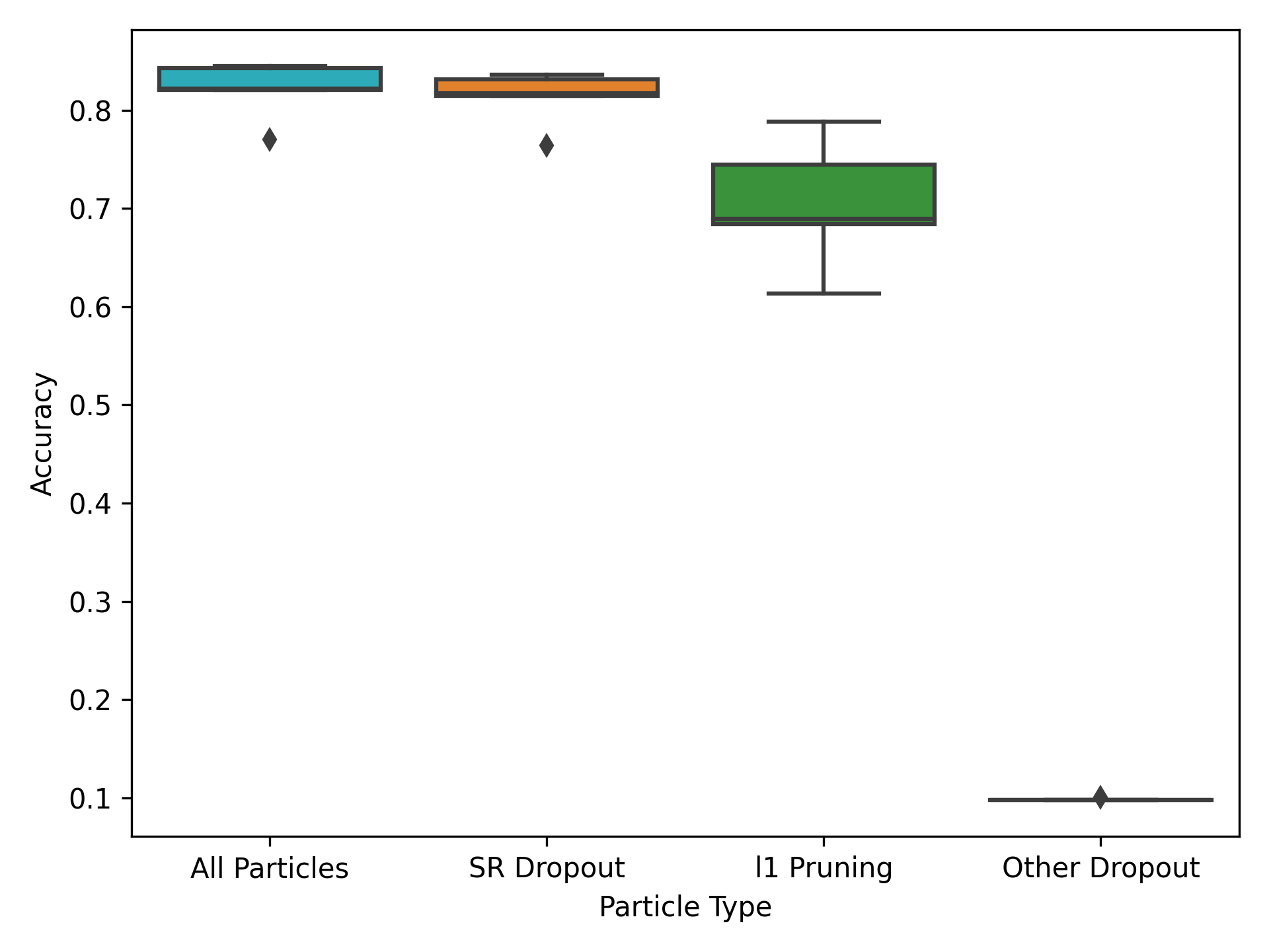
Figure 8: Accuracy (Y-axis) after per-weight-dropout for types $t\in\{PN_{SR},PN_{F}\}$ compared to whole organism and ‘l1-norm’ pruning (X-axis).

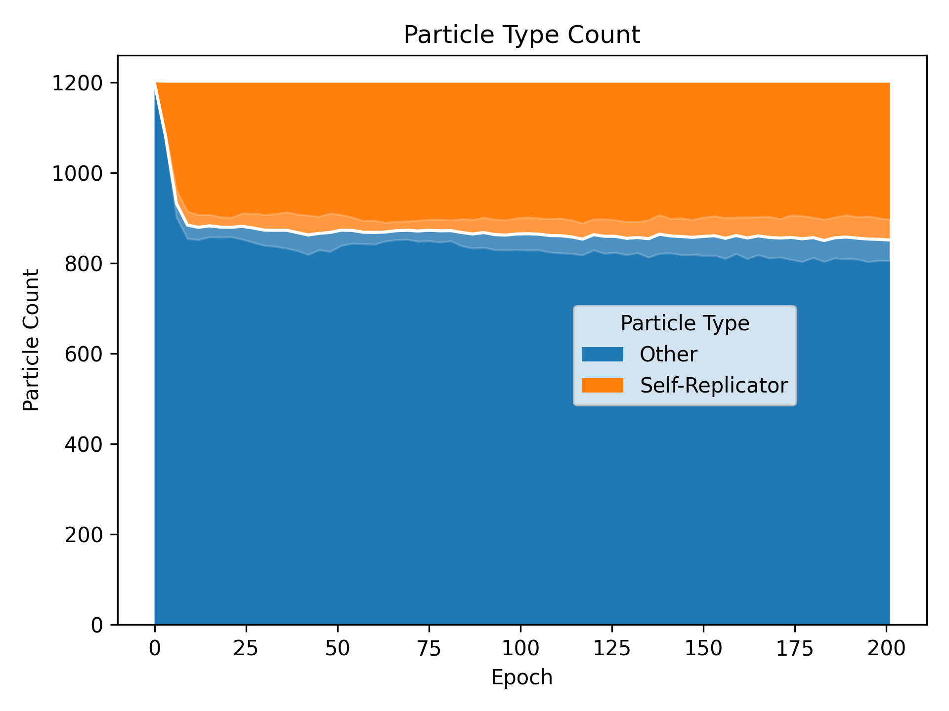
Figure 9: Distribution of PN types ($PN_{SR}$ (orange), $PN_{F}$ (blue); Y-axis) over the course of training the ON on experiment #2, in epochs (X-axis). We observe an initial saturation in the amount of $PN_{SR}$, which then remains roughly stable over the rest of training. We plot the variance over $n=5$ runs with a lighter color to show the consistency of this specialisation development.

Since MNIST allows for a visual exploration, we visualise the positioning of self-replications with SR property. Figure 10a represents the position of $PN_{SR}$ as ‘heatmap’, while Figure 10b is a sum of the approx. weight values (both w.r.t. $x\in X$ each PN is attached to). We find it quite interesting that even the $PN_{SR}$ which are not relevant for the task keep on developing weight representations. Those seem to then get ignored somewhere down the line. This supports our assumption, that $PN_{SR}$ for themselves, ‘realise’ (presumably due to a small gradient) that they are assigned to ‘non-important’ input vectors. For comparison, Figure 10c visualises the per-pixel-mean of the test dataset. We clearly see that replicator specialists ($PN_{SR}$) are mostly responsible for weight predictions of the empty parts of the image around the edges. As MNIST comes with a lot of zero-values, we added Gaussian noise of magnitude $10^{-4}$ to each image. This ensures that the observed behaviour is not simply the result of PNs not being used at all for the AT.

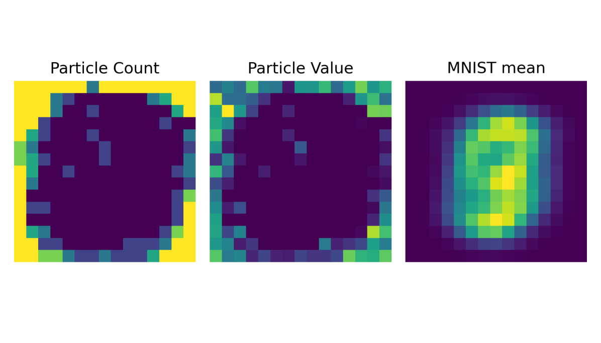
(a) (b) (c)

Figure 10: Heatmap representing the position of found $PN_{SR}$. (a) Per pixel count of $PN_{SR}$ over all $PN$ in the first $ON$-layer. Lighter colour represents more and darker colour fewer $PN_{SR}$ responsible for this input. (b) Per-pixel-sum of the ‘equal-weight-value’ of $PN_{SR}$ overall $PN$ in the first $ON$-layer. (c) Per-pixel-mean of the MNIST dataset for comparison. Here, lighter colour signifies higher values.

Figure 11 visualises the network connectivity per PN-type. This reveals a heavy distribution of $PN_{SR}$ in the input-layer, but not solely. We assume that this positioning is the direct result of ‘non-importance’ in input pixels. leading to much faster convergence for PNs responsible for the image-edge areas. This is quite interesting, as we tried to counter the obvious ‘non-importance’ by adding Gaussian noise, as previously described.

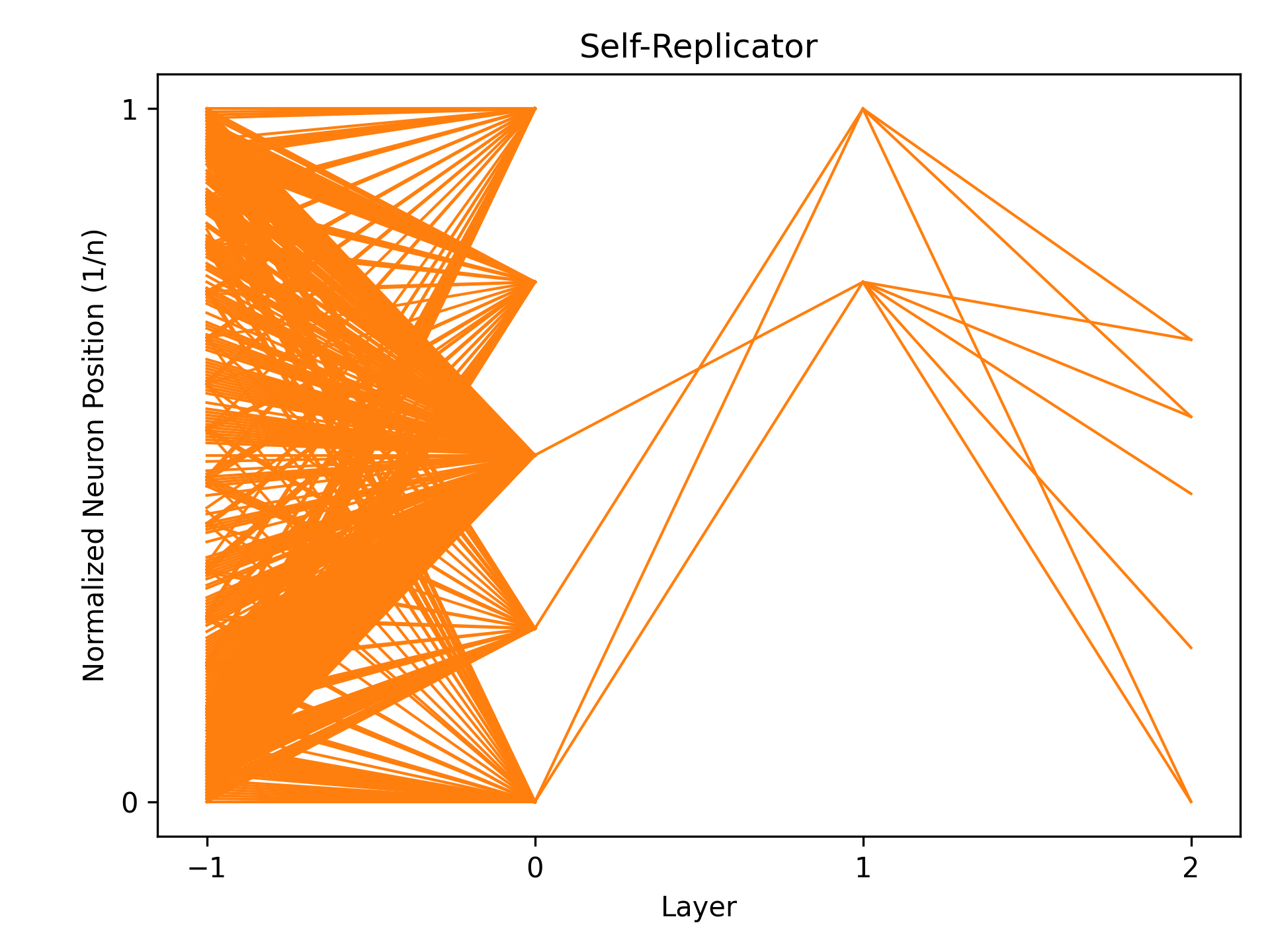
(a)

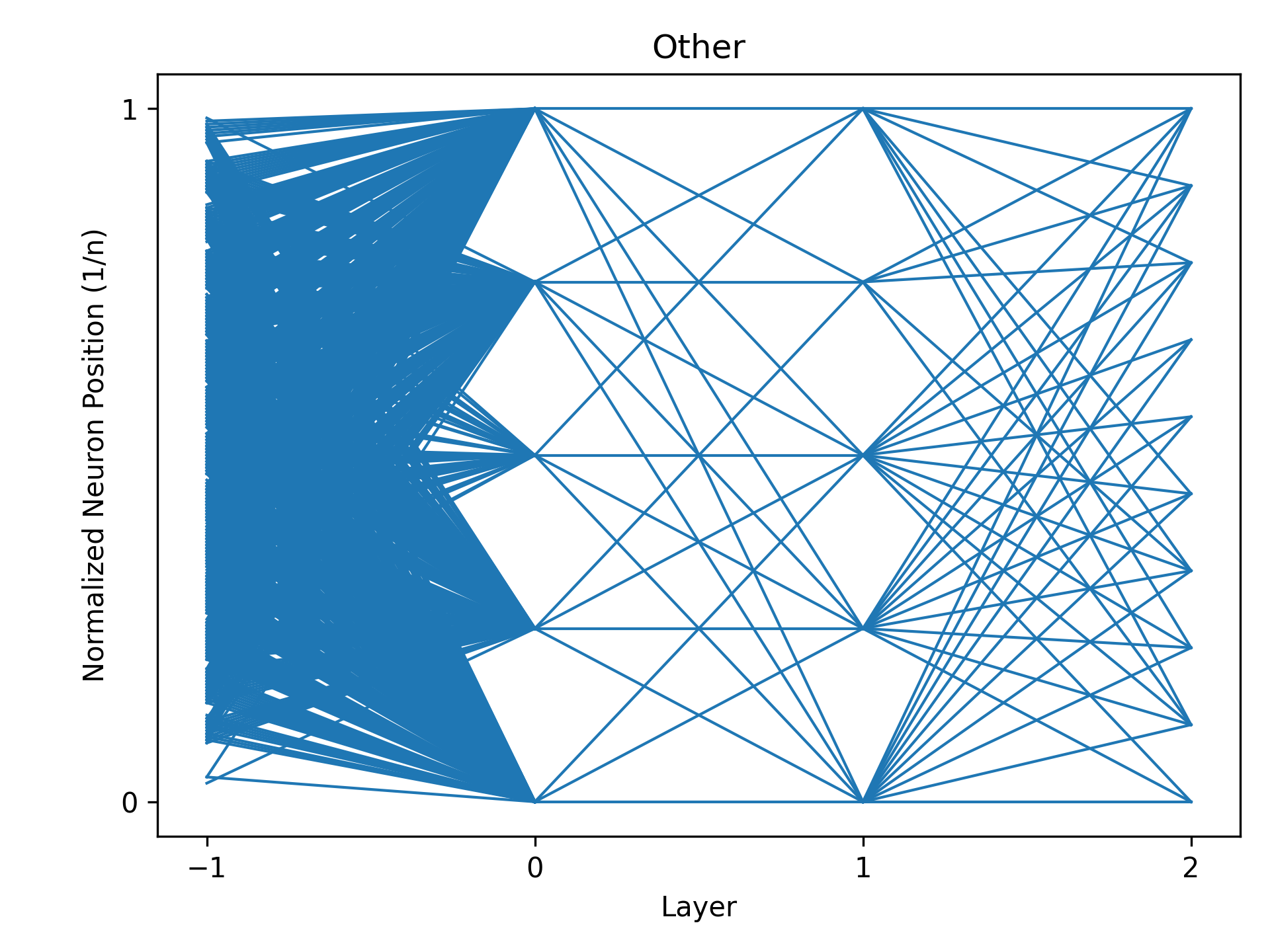
(b)

Figure 11: Connectivity per organism group: (a) pn that have learned the self-replication trait ($PN_{SR}$, orange); (b) pn that have learned the global auxilary task ($PN_{F}$, blue). (Layer #-1 = ON input vector.)

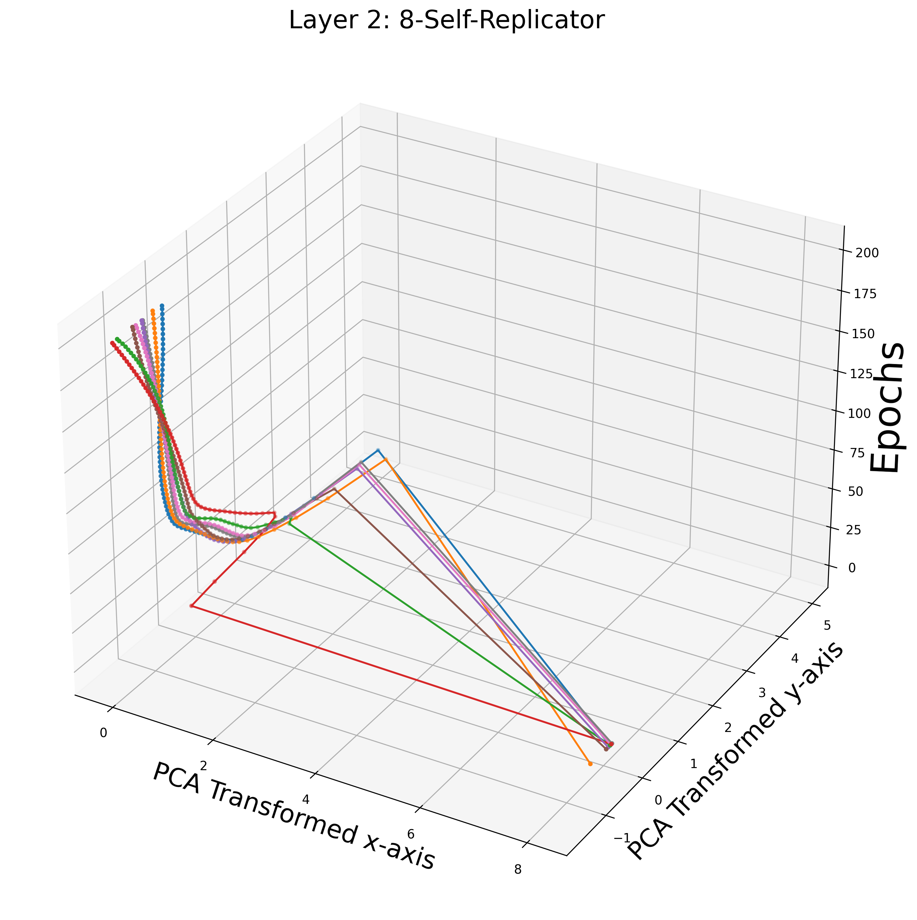
(a)

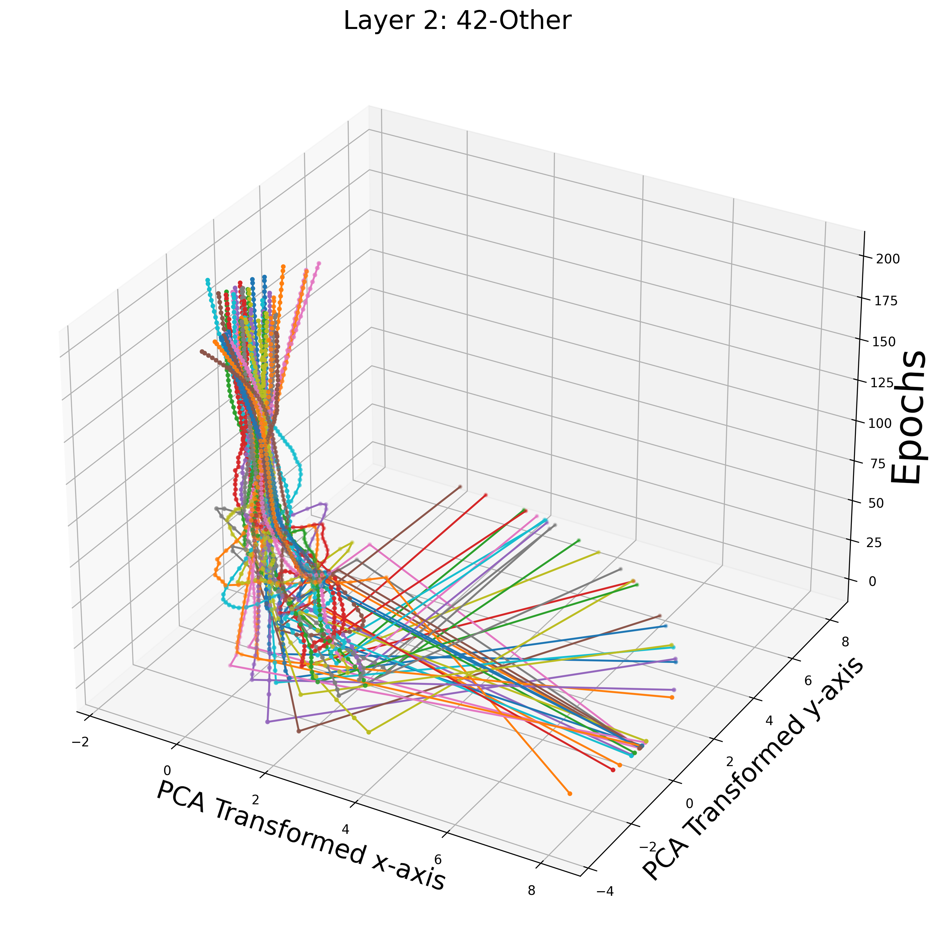
(b)

Figure 12: PCA transformed weight-space trajectories (per PN-group); here Layer 2 of the ON: (a) 8 $PN_{SR}$ that have gained the self-replication-trait; (b) 42 $PN_{F}$ that have learned the auxilary task. Every trajectory (unique colour), shows the change in parameter-values of its corresponding PN.

In the style of Gabor et al. [8, 5] we also take a look at the PCA-transformed weight trajectories per PN-group of an interesting model (cf. Figure 12). Along most of the networks layers (we evaluated more than a single ON), we observe that $PN_{F}$ weight trajectories quickly reach the specific region of their PCA weight space. This is the expected behaviour. Trajectories of $PN_{SR}$, in contrast, are mostly fitted along a single axis by PCA (shared PCA space) (cf. Figure 12a; $layer=2$). This behaviour can also be observed with $PN_{SR}$ in other networks/layers. Please note that we check for trivial fixpoints (e.g., when all weights become zero). Like Gabor et al. [3], we do not consider those ‘self-replicators’ in general but zero-fixpoints. Due to over-plotting, we unfortunately did not learn a lot from PCA trajectories of the heavily populated first layer ($15\times 15\times 5$ PNs; cf. Figure 11).

VI Related Work

Self-replication as a field of research in the context of neural networks receives increasing attention in the past few years. Chang and Lipson [2] developed self-replicating NN quine, which they reviewed on the full MNIST classification task. In contrast to our findings, NN quines seem to lose their ‘incentive’ to receive or hold their SR ability. Our approach in contrast follows the path of optimization to both (local and global) intermixed tasks.

Randazzoo et al. [4] also established a procedure in which they (through back-propagation (BP)) create initial conditions that generate ‘fertile’ self-replicating agents. Training their SR property is achieved by introducing a ‘sink-loss’ which targets a noisy neighbour’s child (network configuration after SA) rather than the network’s own weights, thereby encouraging diverse network replication.

Embedding the replication task into larger structures has – to the best of our knowledge – not been done before. However, the idea of replacing neural nodes with small networks was proposed by CCamp et al. [11], but they focus on the topic of continual learning.  Their deep artificial neurons share one meta-pretrained parameter set that minimizes a memory loss (of previously seen linear regression tasks). Keeping these pretrained parameters fixed, they try to learn (via BP) a weight matrix, connecting the DANs. The focus of this approach is set in favour of the malleability of these ‘vectorized synapses’ (i.e., synaptic plasticity), rather than on the neurons. This two-weight-set approach is part of recent advances in continual learning research, reserving different weight partitions for task memory: Ba et al. [12], e.g., present the benefits of using 2 synaptic weight sets with novel ‘fast weights’ for improved knowledge retention. More recently, Hurtado et al. [13] proposed specific shared weights as a common knowledge base between tasks. Our work, in contrast, does not check for the memory of tasks or explicitly assign task positions, but rather aims to train dual-purpose particles right from the start. We also do not keep any part of the organism fixed, but we do second the choice of utilizing small neuron particles, especially since Beniaguev et al. [14] have shown that (even small) multi-layer networks suffice in mimicking the functionality of real cortical neurons.

The process of removing the $PN_{SR}$ from the trained ON (cf. our post-training dropout test) is comparable to the concept of selecting important network weights in the context of NN pruning. For a broad overview, please refer to Blalock et al. [15]. This is of interest as, on the one hand, modern network architectures are assumed to be prone to over-parameterization [16]. However, on the other hand, recent research suggests that there are subsets of parameter configurations with (at least) equal test accuracy (compared to the original network) in any randomly initialized, dense neural network [17]. Locating these excess parameters via specialisation in different tasks as shown in this work could form the ‘natural-selection’ counterpart to simple value threshold pruning commonly in use (e.g., see Zhu and Gupta [18]).

Our approach of utilizing small, randomly initialized networks in a larger meta-structure to predict connectivity results also shares similarity with the network kernel recently introduced by Amid et al. [19], which returns the expected inner-product of the network logits given some input samples. Lin et al. [20] also employ a secondary ‘micro’ network as a function approximator in-between layers, albeit focused on a convolutional network architecture. We use a simple architecture, as Tolstikhin et al. [21] have shown the sufficient potency of multi-layer perceptron (MLP) architectures for vision tasks.

Finally, with each of our organism network also training themselves independently, we point to the Particle Swarm Optimization (PSO) algorithm (see Carvalho and Ludermir [22]) as conceptually related work, which changes and improves its network parameters by iterating through fitness-based points in solution space (particles).

VII Conclusion and Future Work

In this work, we built a cooperating organism network made from cells of ‘self-replicators’ to introduce the field of SRNN-research to real-world tasks and explore the findings along the way. Our approach employs SRNN as weight approximators for a greater computational graph (NN). We achieved our goal in training the ON (which is made up of smaller groups of particles) in an end-to-end fashion. We show a simple proof-of-concept goal (float-number addition) as well as a non-trivial task (MNIST image classification) to work respectably well.

On our way, we have found that the particles can become robust goal-networks themselves, i.e., SRNNs performing both self-replication and MNIST classification. This dual status becomes harder to reach as PNs are utilised in more complex group actions. For the image classification task, we see the emergence of this dual-ability occurring primarily in particles responsible for areas of low importance in the input, signaling the ‘leisure’ to specialise into both tasks.

As PNs represent an approximation of the weight scalar, we can deduct the weight value activating each particle, allowing us to populate conventional feed-forward NN layers. When pruning parameters on corresponding positions (to $PN_{SR}$) of a comparable NN we observe minimal test-accuracy loss, which seems to outperform simple ‘l1-norm’ pruning. For the future, it remains interesting to work on exploring further aspects of learned self-regulation within the organism network, e.g., the usage of particles as learned cell aggregators or layer activation function approximators. Furthermore, operator-based interaction between particles has to be further explored.

The option to scale up training and input dimensions for the organism network is also a priority. As our networks stayed relative simple w.r.t. to the architecture, function, and training regime, there is a lot of methodology from the well-established field of ‘deep learning’ that we did not touch yet. Other directions for further research are a more in-depth examination of the viability of different data-sets on the training ability of the organisms. Although we have shown the importance-selection to work also with a noisy rendition of MNIST, it will be interesting to see the impact of RGB data without any dead-spots (i.e., CIFAR10). We leave those considerations as well as further tests and comparisons of mentioned pruning strategies discussed in related work (repeated training, self-pruning, fine-tuning) for the future.

References

- [1] S. A. Kauffman et al., The origins of order: Self-organization and selection in evolution. Oxford University Press, USA, 1993.
- [2] O. Chang and H. Lipson, “Neural network quine,” in Artificial Life Conference Proceedings, MIT Press, 2018.
- [3] T. Gabor, S. Illium, A. Mattausch, L. Belzner, and C. Linnhoff-Popien, “Self-replication in neural networks,” in ALIFE 2019: The 2019 Conference on Artificial Life, pp. 424–431, MIT Press, 2019.
- [4] E. Randazzo, L. Versari, and A. Mordvintsev, “Recursively fertile self-replicating neural agents,” in ALIFE 2021: The 2021 Conference on Artificial Life, MIT Press, 2021.
- [5] T. Gabor, S. Illium, M. Zorn, and C. Linnhoff-Popien, “Goals for self-replicating neural networks,” in ALIFE 2021: The 2021 Conference on Artificial Life, MIT Press, 2021.
- [6] Y. LeCun, Y. Bengio, and G. Hinton, “Deep learning,” Nature, vol. 521, pp. 436–44, 05 2015.
- [7] D. E. Rumelhart, G. E. Hinton, and R. J. Williams, “Learning representations by back-propagating errors,” nature, vol. 323, no. 6088, pp. 533–536, 1986.
- [8] T. Gabor, S. Illium, M. Zorn, C. Lenta, A. Mattausch, L. Belzner, and C. Linnhoff-Popien, “Self-Replication in Neural Networks,” Artificial Life, pp. 205–223, 06 2022.
- [9] L. Deng, “The mnist database of handwritten digit images for machine learning research,” IEEE Signal Processing Magazine, vol. 29, no. 6, pp. 141–142, 2012.
- [10] D. Hendrycks and K. Gimpel, “Gaussian error linear units (gelus),” arXiv preprint arXiv:1606.08415, 2016.
- [11] B. Camp, J. K. Mandivarapu, and R. Estrada, “Continual learning with deep artificial neurons,” arXiv preprint arXiv:2011.07035, 2020.
- [12] J. Ba, G. E. Hinton, V. Mnih, J. Z. Leibo, and C. Ionescu, “Using fast weights to attend to the recent past,” Advances in neural information processing systems, vol. 29, 2016.
- [13] J. Hurtado, A. Raymond, and A. Soto, “Optimizing reusable knowledge for continual learning via metalearning,” Advances in Neural Information Processing Systems, vol. 34, pp. 14150–14162, 2021.
- [14] D. Beniaguev, I. Segev, and M. London, “Single cortical neurons as deep artificial neural networks,” Neuron, vol. 109, no. 17, pp. 2727–2739, 2021.
- [15] D. Blalock, J. J. Gonzalez Ortiz, J. Frankle, and J. Guttag, “What is the state of neural network pruning?,” Proceedings of machine learning and systems, vol. 2, pp. 129–146, 2020.
- [16] M. Denil, B. Shakibi, L. Dinh, M. Ranzato, and N. De Freitas, “Predicting parameters in deep learning,” Advances in neural information processing systems, vol. 26, 2013.
- [17] J. Frankle and M. Carbin, “The lottery ticket hypothesis: Finding sparse, trainable neural networks,” arXiv preprint arXiv:1803.03635, 2018.
- [18] M. Zhu and S. Gupta, “To prune, or not to prune: exploring the efficacy of pruning for model compression,” arXiv preprint arXiv:1710.01878, 2017.
- [19] E. Amid, R. Anil, W. Kotłowski, and M. K. Warmuth, “Learning from randomly initialized neural network features,” arXiv preprint arXiv:2202.06438, 2022.
- [20] M. Lin, Q. Chen, and S. Yan, “Network in network,” arXiv preprint arXiv:1312.4400, 2013.
- [21] I. O. Tolstikhin, N. Houlsby, A. Kolesnikov, L. Beyer, X. Zhai, T. Unterthiner, J. Yung, A. Steiner, D. Keysers, J. Uszkoreit, et al., “Mlp-mixer: An all-mlp architecture for vision,” Advances in Neural Information Processing Systems, vol. 34, 2021.
- [22] M. Carvalho and T. B. Ludermir, “Particle swarm optimization of neural network architectures and weights,” in 7th International Conference on Hybrid Intelligent Systems (HIS 2007), pp. 336–339, IEEE, 2007.