A Rigorous Framework for Automated Design Assessment and Type I Error Control: Methods and Demonstrative Examples (Working Paper)

1 Abstract

We present a “proof-by-simulation” framework for rigorously controlling a trial design’s operating characteristics over continuous regions of parameter space. We show that proof-by-simulation can achieve two major goals: (1) Calibrate a design for provable Type I Error control at a fixed level $\alpha$. (2) Given a fixed design, bound (with high probability) its operating characteristics, such as the Type I Error, FDR, or bias of bounded estimators. This framework can handle adaptive sampling, nuisance parameters, administrative censoring, multiple arms, and multiple testing. These techniques, which we call Continuous Simulation Extension (CSE), were first developed in Sklar (2021) to control Type I Error and FWER for designs where unknown parameters have exponential family likelihood. Our appendix improves those results with more efficient bounding and calibration methods, extends them to general operating characteristics including FDR and bias, and extends applicability to include canonical GLMs and some non-parametric problems. In the main paper we demonstrate our CSE approach and software on 3 examples: (1) a gentle introduction, analyzing the z-test (2) a hierarchical Bayesian analysis of 4 treatments, with sample sizes fixed (3) an adaptive Bayesian Phase II-III selection design with 4 arms, where interim dropping and go/no-go decisions are based on a hierarchical model. Trillions of simulations were performed for the latter two examples, enabled by specialized INLA software. Open-source software is maintained at [1].

2 Introduction

An experiment plan must account for many unknowns: treatment effect sizes, enrollment rates, modeling assumptions, nuisance parameters, and more. To ensure robustness, prevent bluffing, and protect against adversarial design optimization, regulators and designers should analyze the design not only in the expected case, but across a wide space of possible cases.

The classical approach is to use mathematical techniques, primarily Type I Error proofs and techniques based on Gaussian approximations to the log-likelihood, to control the design’s operating characteristics. But the complexity of modern design can often break these standard tools, for reasons including:

1. Slow central-limit convergence in finite samples.

2. Non-Gaussian limit behavior due to adaptive sampling. (The resulting limiting distributions are usually non-pivotal, which causes the bootstrap to fail [2].)

3. Difficult or absent mathematical asymptotics (such as for Bayesian decisionmaking, bandit algorithms, or models with nuisance parameters).

4. Nuisance parameters, adaptive design plans with enrollment uncertainty, or protocol changes which add or drop treatment arms.

Various theoretical remedies to these issues have been proposed, including: edgeworth and saddlepoint expansions [3] for (1); hybrid resampling [4] for (1) and (2); dynamic programming and index policies [5] for (1) (2) and (3); diffusion asymptotic limits for certain adaptive sampling schemes [6, 7] for (2) and (3); and combination tests combined with closed testing [8] for (4). However for highly complex designs, these approaches may face implementation difficulties or even fail, particularly for cases with nuisance parameters and/or multiple treatments.

In practical work, simulation has risen to the status of a core technology for addressing these challenges. The FDA Complex Innovative Trial Design Meeting Program (CID) currently uses simulation to validate “complex adaptive, Bayesian, and other novel clinical trial designs.” [9]. Simulation is also a key underpinning of trial design packages such as RCTdesign [10] and FACTS [11].

In this work, building on ideas from [12], we propose a new approach called Continuous Simulation Extension (CSE), which can upgrade simulations of operating characteristics taken at fixed parameter values into bounds that hold rigorously over regions of parameter space. CSE can be applied to wide classes of distributions, including exponential families, canonical form GLMs, and some non-parametric models. This technique allows us to perform two main tasks:

1. Given a fixed design, provide a lower or upper-bound on quantities such as Type I Error, false-discovery rate (FDR), or bias of bounded estimators over a (bounded) parameter space with a pointwise-valid confidence bound with confidence parameter $\delta$. This process is introduced in Section 3.1 and rigorously described in Appendix A.

2. Calibrate the critical threshold of a design to achieve a provable bound on the expected Type I Error of the selected threshold on a (bounded) parameter space. That is, we show how to select a (random) critical threshold, denoted $\hat{\lambda}^{*}$, such that

   $$\forall\theta\in\Theta,\,\mathbb{E}\left[f_{\hat{\lambda}^{*}}(\theta)\right]\leq\alpha$$

   where $f_{\lambda}(\theta)$ is the Type I Error of the design with critical threshold $\lambda$ under parameter $\theta$, and $\Theta$ is the null hypothesis region of parameter values. This process is introduced in Section 3.2 and fully described in Appendix B.

Thus, CSE can provide rigorous validation of a quality on par with classical proofs. Moreover, these bounding guarantees are non-asymptotically valid, with a loss-to-conservativeness which can be driven toward zero with increasing simulation scale.

For takeaways and commentary, the reader may jump straight to Section 7 (Discussion). The remainder of this paper focuses on explaining the core methodology and results on 3 examples. In Section 3, we introduce CSE with a familiar example, the z-test. In Sections 4 and 5 respectively, we analyze two design examples, both with Bernoulli outcomes: a Phase II basket trial (Section 4) and a complex Phase II-III design with Bayesian analyses and interim decision-making based on conditional power (Section 5). Section 6 describes the contents of supplementary materials, which contain the rigorous mathematical derivations. Open-source code for the first example is published at [1].

3 CSE Tutorial Example: The Z-Test

In this section, we demonstrate CSE in the familiar setting of the z-test. We analyze the Type I Error of the one-sided z-test with critical value $z^{*}:=z_{1-\alpha}$ for the target level $\alpha=2.5\%$. That is, our data is a single draw $Z\sim N(\theta,1)$, where $\theta$ is an unknown scalar parameter, and our test rejects if $Z>z^{*}$. Traditionally, the null hypothesis space is $\theta\in(-\infty,0].$ For simplicity and computational boundedness, we limit our attention to $\theta\in\Theta:=[-1,0]$.

Section 3.1 explains the validation procedure and Section 3.2 explains the calibration procedure as we use these methods on the z-test.

3.1 Validation Procedure

The validation procedure uses simulation to construct pointwise-valid confidence bands on the Type I Error of a fixed design, over a (bounded) parameter space. That is, for any $\delta\in(0,1)$, we wish to construct lower and upper bounds $l(\theta),u(\theta)$ from simulations that satisfy the following property:

$$\forall\theta\in\Theta,\, \mathbb{P}\left(f(\theta)>u(\theta)\right)\leq\frac{\delta}{2}$$

$$\mathbb{P}\left(f(\theta)<l(\theta)\right)\leq\frac{\delta}{2}$$

where $f(\theta)$ is the Type I Error. Thus, at each value of $\theta$, the pair $(l(\theta),u(\theta))$ is a valid $(1-\delta)$ confidence interval about the true Type I Error.

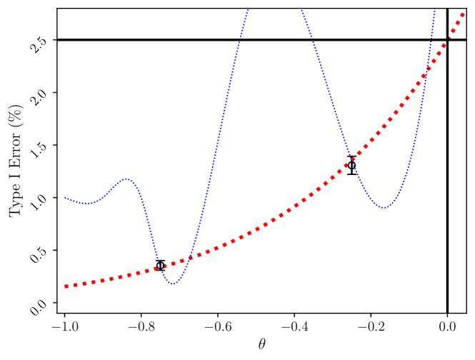
Figure 1: Clopper-Pearson confidence intervals of the Type I Error are constructed at $\theta\in\{-0.75,-0.25\}$ (black vertical bars). The true Type I Error (red dotted line) is drawn with an arbitrarily complex function (blue dotted line) that passes through the confidence interval bounds.

To construct the confidence band, we begin with a grid of points, $\{\theta_{i}\}_{i=1}^{I}\subseteq\Theta$. For example, in Figure 1, the set of grid-points is $\{-0.75,-0.25\}$. We repeatedly simulate the test procedure at each $\theta_{i}$ and construct the $(1-\delta)$ Clopper-Pearson bounds of the Type I Error. This controls the Type I Error at every $\theta_{i}$; however, the question remains: how to extend this control to other points $\theta\in\Theta\setminus\{\theta_{i}\}_{i=1}^{I}$? In this case, the true Type I Error function, represented by the red dotted line in Figure 1, is indeed well-behaved and controlled at level $\alpha$. But a critic could ask: what if an irregular function such as the blue dotted line passes through the Type I Error confidence intervals yet exceeds $\alpha$ in between? We would like to rigorously rule out such aberrant functions.

To achieve this, we introduce the Tilt-Bound, a family of inequalities which, given a fixed event $A$, tightly bounds $\mathbb{P}_{\theta}\left(A\right)$ for $\theta$ in the neighborhood of a fixed parameter value $\theta_{0}$. Formally, the Tilt-Bound is a function $U(\theta_{0},v,q,a)$ that provides the following inequality for a displacement $v$ and parameter $q\geq 1$:

$$f(\theta_{0}+v) \leq U(\theta_{0},v,q,f(\theta_{0}))$$

Then, denoting $\hat{u}$ as the Clopper-Pearson upper bound at $\theta_{0}$ and using that $a\mapsto U(\theta_{0},v,q,a)$ is increasing,

$$\mathbb{P}\left(f(\theta_{0}+v)>U(\theta_{0},v,q,\hat{u})\right) \leq\mathbb{P}\left(f(\theta_{0})>\hat{u}\right)\leq\frac{\delta}{2}$$

This shows that we may take the upper bound function

$$u(\theta):=U(\theta_{i},\theta-\theta_{i},q,\hat{u}_{i})$$

where $\theta_{i}$ is any simulation grid-point and $\hat{u}_{i}$ is the Clopper-Pearson upper bound estimate at $\theta_{i}$, to achieve a pointwise-valid confidence guarantee over $\Theta$. Typically, we choose $\theta_{i}$ closest to $\theta$. If desired, a lower bound can be constructed similarly. The Tilt-Bound is formally stated in Theorem 1 and extensively discussed in Appendix A. The Tilt-Bound bears similarity to the Taylor expansion bounds of [12], but instead relies on Hölder’s Inequality to develop a family of bounds indexed by a parameter $q\in[1,\infty]$. Since the bound holds for every $q\in[1,\infty]$, it can also be minimized over $q$ for sharper results. With exponential family data, the Tilt-Bound formula is:

$$U(\theta_{0},v,q,f(\theta_{0})) =f(\theta_{0})^{1-\frac{1}{q}}\exp\left[\frac{A(\theta_{0}+qv)-A(\theta_{0})}{q}-\left(A(\theta_{0}+v)-A(\theta_{0})\right)\right]$$

where $A(\theta)$ is the log-partition function of the exponential family. Applying this to the normal family $\{\operatorname{\mathcal{N}}\left(\theta,1\right):\theta\in\Theta\}$ which is an exponential family with log-partition function $A(\theta)=\frac{\theta^{2}}{2}$, the Tilt-Bound simplifies to:

$$U(\theta_{0},v,q,f(\theta_{0})) =f(\theta_{0})^{1-\frac{1}{q}}\exp\left[\frac{(q-1)v^{2}}{2}\right]$$ (1)

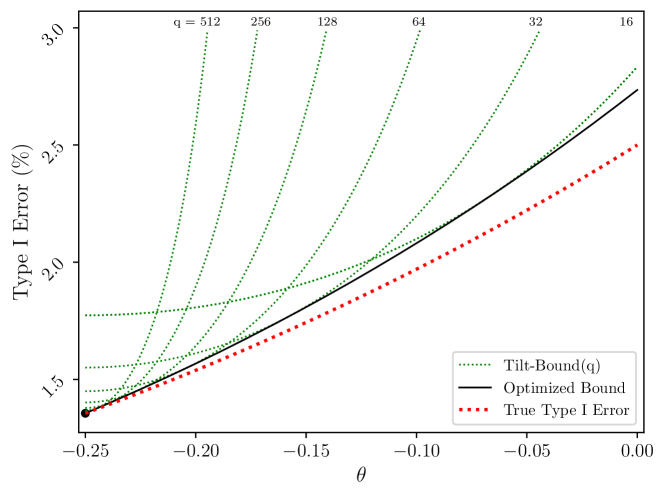
Figure 2: The normal Tilt-Bound (1) for various fixed values of $q$ (green dotted lines) are overlaid with the optimal Tilt-Bound (black solid line), which optimizes for $q$ at every $\theta$. It has been assumed that the true Type I Error at the initial point $\theta_{0}=-0.25$ is known correctly to plug into the bound. As a baseline comparison, we plot the true Type I Error (red dotted line). In this case, the bound is only mildly conservative, although the slack grows with distance from the initial point.

In Figure 2, we plot the Tilt-Bound for various fixed values of $q$ and overlay the optimized Tilt-Bound. Note that the optimal choice of $q$ can vary for different displacements from the fixed grid-point $\theta_{0}=-0.25$. The comparison between the optimized Tilt-Bound and the true Type I Error shows that the difference is quite small even for large displacements. Moreover, we see that any fixed value of $q$ provides an undesirably loose bound away from the minimum, i.e. the optimal Tilt-Bound is significantly tighter to the Type I Error than the Tilt-Bound with a fixed value $q$. We also observe that the bound increases with distance, so that the worst case occurs at an edge. For example, in Figure 2, the worst-case occurs at $\theta\equiv 0$. More generally, Lemma 2 shows a similar result holds in higher dimensions: if the set of displacements considered is a polytope, then the worst-case occurs at a vertex.

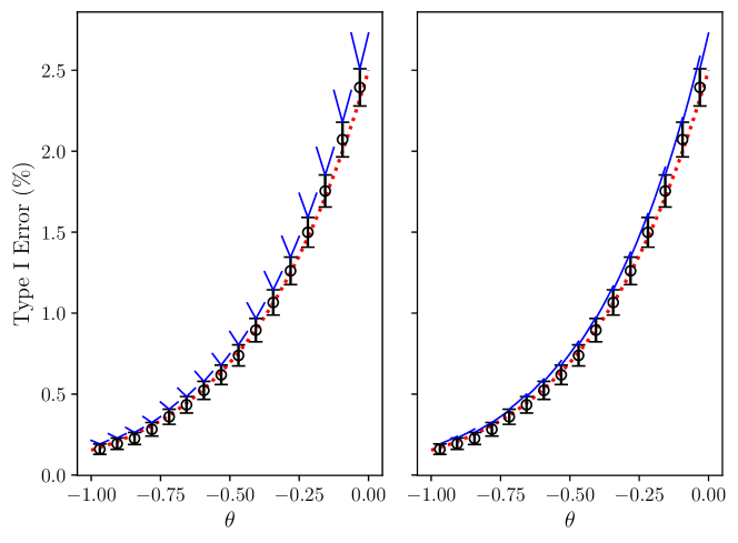
Figure 3: Plot of the optimized Tilt-Bound (blue solid line) for the z-test using 16 equally-spaced simulation points and Clopper-Pearson confidence intervals (black vertical bars) overlaid with the true Type I Error (red dotted line). The left constructs the Tilt-Bound using each simulation point as the center of an interval. The right constructs the Tilt-Bound using each simulation point as the left end-point of an interval.

Figure 3 shows the Tilt-Bound results for the z-test using only 16 simulation points. We choose equally-spaced 16 points in the interval $(-1.0,0.0)$ and construct $(1-\delta)$ Clopper-Pearson intervals at each point, where $\delta\equiv 0.05$. For each grid-point, we construct the optimized Tilt-Bound around the grid-point using the Clopper-Pearson upper bound value. In the figure, the first method (left) uses the grid-point as the center and extrapolates to both left and right of it, and the second method (right) uses the grid-point as the left end-point and extrapolates only to the right. For the given normal family, due to isotropy of the Gaussian family, the bound (1) is symmetric for negative and positive displacements. Hence, the second method is technically a tighter bound than the first method in the figure. However, both methods provide valid confidence intervals and are similar in the areas with the highest Type I Error, which are the regions of primary concern.

To summarize, the validation procedure is the following steps:

Algorithm 1 Validation Procedure

1:Partition the (bounded) null hypothesis space $\Theta$ into tiles $A_{i}\subseteq\Theta$.

2:Assign to each $A_{i}$ a central point $\theta_{i}$.

3:Construct a $(1-\delta)$ Clopper-Pearson interval at $\theta_{i}$.

4:Use the optimized Tilt-Bound to extend the confidence interval at $\theta_{i}$ to all points in $A_{i}$.

We conclude this section with a few remarks on our approach. By increasing the number of simulations, we can tighten the Clopper-Pearson bounds at each $\theta_{i}$. And by increasing the granularity of the grid-points, i.e. by making the tiles smaller, the error of the Tilt-Bound decreases. Although we restricted the null hypothesis space to a bounded set, this assumption is mild one. In some cases, analytic arguments can provide coverage over the remainder of the space.

3.2 Calibration Procedure

The calibration procedure will provably control the Type I Error on a (bounded) parameter space $\Theta$. Note that the validation procedure described in Section 3.1 is not sufficient to guarantee Type I Error at a fixed $\alpha$ level: for example, if the true Type I Error is $\alpha$, the Clopper-Pearson confidence interval could contain values greater than $\alpha$ due to simulation error. Moreover, the confidence interval only holds with probability $1-\delta$, and hence, can only give probabilistic guarantees. The calibration procedure improves on all these issues, achieving a fixed level guarantee. At a high-level, the procedure selects a random critical threshold for a given design such that the expected Type I Error with the selected threshold is controlled at $\alpha$ on all of $\Theta$. (Appendix B provides a rigorous analysis.)

To understand the calibration procedure, it is best to start by considering a single point null $\theta_{0}$. Assuming $N$ simulations are performed at $\theta_{0}$ and the test statistic has a continuous distribution, standard results based on the Beta distribution yield the following result: if one selects a rejection threshold $\hat{\lambda}^{*}$ such that it rejects $\lfloor(N+1)\alpha\rfloor$ of the simulations, then using this threshold yields an expected rejection probability of $\frac{\lfloor(N+1)\alpha\rfloor}{N+1}$ at $\theta_{0}$. Mathematically: letting the Type I Error at $\theta$ with critical threshold $\lambda$ be denoted

$$f_{\lambda}(\theta):=\mathbb{P}_{\theta}\left(S(X)<\lambda\right)$$

for some test statistic $S(X)$, Theorem 8 shows that

$$\mathbb{E}_{\theta_{0}}\left[f_{S_{(k)}}(\theta_{0})\right]\leq\frac{k}{N+1}$$

where $S_{1},\ldots,S_{N}$ are $N$ i.i.d. test statistics under parameter $\theta_{0}$, and $S_{(k)}$ is the $k$’th order statistic. Hence, this result allows us to target a Type I Error upper bound at a given point at any level $\alpha^{\prime}$ by setting $k=\lfloor(N+1)\alpha^{\prime}\rfloor$ and choosing the (random) threshold

$$\hat{\lambda}^{*}:=S_{(\lfloor(N+1)\alpha^{\prime}\rfloor)}$$ (2)

Using the calibration result at a fixed parameter $\theta_{0}$, we can extend the level $\alpha^{\prime}$ guarantee to a region around $\theta_{0}$. For any random rejection rule $\hat{\lambda}^{*}$, it can be shown that the Tilt-Bound can also be applied (see Appendix B) so that

$$\mathbb{E}\left[f_{\hat{\lambda}^{*}}(\theta_{0}+v)\right] \leq U(\theta_{0},v,q,\mathbb{E}\left[f_{\hat{\lambda}^{*}}(\theta_{0})\right])$$ (3)

for any $q\geq 1$. Letting $H$ be the set of displacements from $\theta_{0}$, we may back-solve (3) for $\mathbb{E}\left[f_{\hat{\lambda}^{*}}(\theta_{0})\right]$ so that the Type I Error is controlled at $\alpha$ everywhere in $\theta_{0}+H$, i.e.

$$\sup\limits_{v\in H}\mathbb{E}\left[f_{\hat{\lambda}^{*}}(\theta_{0}+v)\right]\leq\alpha$$ (4)

Specifically, (4) holds so long as

$$\mathbb{E}\left[f_{\hat{\lambda}^{*}}(\theta_{0})\right] \leq\inf\limits_{v\in H}U^{-1}(\theta_{0},v,q,\alpha)$$ (5)

where

$$U^{-1}(\theta_{0},v,q,\alpha) =\left(\alpha\exp\left[-\frac{A(\theta_{0}+qv)-A(\theta_{0})}{q}+A(\theta_{0}+v)-A(\theta_{0})\right]\right)^{\frac{q}{q-1}}$$ (6)

for an exponential family. For the normal family $\{\operatorname{\mathcal{N}}\left(\theta,1\right):\theta\in\Theta\}$, (6) further simplifies to:

$$U^{-1}(\theta_{0},v,q,\alpha) =\left(\alpha\exp\left[-\frac{(q-1)v^{2}}{2}\right]\right)^{\frac{q}{q-1}}$$ (7)

The inverted Tilt-Bound (6) can be thought of as a target to ensure the test $\theta_{0}+v$ will be level $\alpha$, since

$$\mathbb{E}\left[f_{\hat{\lambda}^{*}}(\theta_{0})\right]\leq U^{-1}(\theta_{0},v,q,\alpha)\implies\mathbb{E}\left[f_{\hat{\lambda}^{*}}(\theta_{0}+v)\right]\leq\alpha$$

by (3). As in Section 3.1, we may maximize (5) over $q\geq 1$ to reduce the Type I Error lost to conservativeness at $\theta_{0}$. Hence, letting

$$\alpha^{\prime}\equiv\sup\limits_{q\geq 1}\inf\limits_{v\in H}U^{-1}(\theta_{0},v,q,\alpha)$$ (8)

and using the previous results to choose $\hat{\lambda}^{*}:=S_{\lfloor(N+1)\alpha^{\prime}\rfloor}$ under $\theta_{0}$, we have control at level $\alpha$ on all of $H+\theta_{0}$.

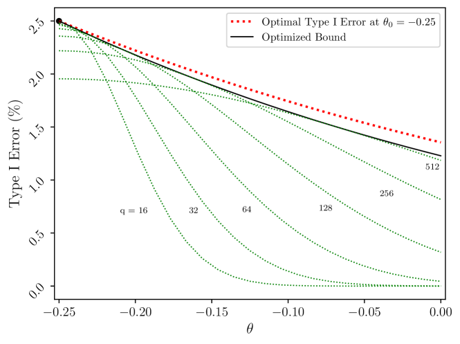
Figure 4: The normal inverted Tilt-Bound (7) for various fixed values of $q$ (green dotted lines), overlaid with the optimal inverted Tilt-Bound (black solid line) which optimizes for $q$ at every $\theta$. We compute the inverted bound using $\theta_{0}=-0.25$ with a target of $\alpha=2.5\%$. The inverted Tilt-Bound evaluated at $\theta$ is a target Type I Error bound at $\theta_{0}$ such that the Type I Error at $\theta$ would be guaranteed to be under $\alpha$. As a baseline comparison, we plot the optimal Type I Error (red dotted line) at $\theta_{0}$ using the rejection threshold that exactly hits $\alpha$ at a given $\theta$.

In Figure 4, we plot the inverted Tilt-Bound for the normal family (7) for various fixed values of $q$ overlaid with the optimized bound. We consider $\theta_{0}=-0.25$ and target level $\alpha=0.025$. As in Section 3.1, the optimal choice of $q$ varies depending on the displacement from the fixed grid-point $\theta_{0}$. Similar to the Tilt-Bound, the inverted Tilt-Bound for fixed $q$ also enjoys the same property that the worst-case (smallest) bound occurs at the boundary of a bounded set and occurs at a vertex for a polytope. We see that at $\theta\equiv\theta_{0}$, the optimal bound is exactly $\alpha$, since there is no approximation error from the bound. As $\theta$ moves away from $\theta_{0}$, the optimal bound shrinks. One can measure the amount of slack lost due to the bound at any $\theta$ by comparing the inverted Tilt-Bound with the Type I Error of a test at $\theta_{0}$ such that the Type I Error at $\theta$ hits exactly $\alpha$. Specifically, we plot the “optimal” Type I Error at $\theta_{0}$

$$1-\Phi\left(\Phi^{-1}(1-\alpha)+\theta-\theta_{0}\right)$$

in dotted red where $\Phi$ is the cumulative distribution function for the standard normal. In all cases, the bound is no larger than the optimal Type I Error, which is expected. However, in this example, the difference between them is small, so the resulting calibrated test is only mildly conservative. In general, the level of conservativeness depends largely on how far $\theta$ is from $\theta_{0}$, i.e. the larger the distance between $\theta_{0}$ and $\theta$, the more conservative the test is. Similar to the validation procedure, this issue is remedied by creating more grid-points so that each one does not have to extrapolate far.

For a general (bounded) null hypothesis space $\Theta$, the calibration procedure is described in Algorithm 2. Algorithm 2 produces a random threshold $\hat{\lambda}^{*}$ such that

$$\sup\limits_{\theta\in\Theta}\mathbb{E}\left[f_{\hat{\lambda}^{*}}(\theta)\right]\leq\alpha$$

Algorithm 2 Calibration Procedure

1:Partition the (bounded) null hypothesis $\Theta$ into tiles $A_{i}\subseteq\Theta$.

2:Assign to each $A_{i}$ a central point $\theta_{i}$.

3:Back-solve (5) for each $\theta_{i}$ with optimal $q$ to get $\alpha^{\prime}_{i}$ as in (8).

4:Calibrate the design at each $\theta_{i}$ by choosing a random threshold $\hat{\lambda}_{i}^{*}$ as in (2).

5:Select the most conservative threshold $\hat{\lambda}^{*}:=\min\limits_{i}\hat{\lambda}^{*}_{i}$.

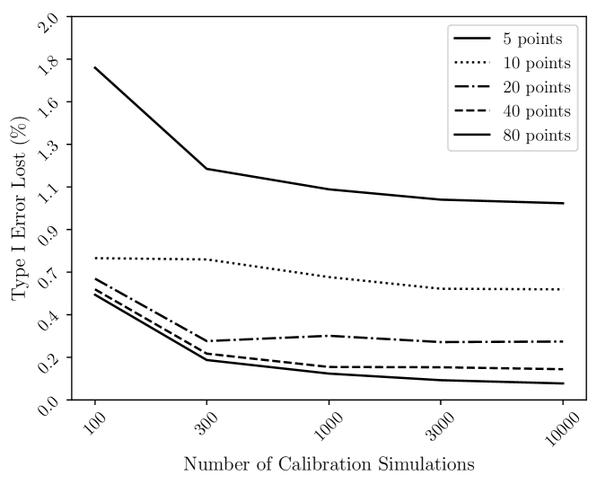
Figure 5: Plot of the average conservativeness of the calibrated z-test for a range of different number of grid-points. The y-axis is the difference between the true Type I Error of the optimal z-test and the worst-case average Type I Error using the threshold (2), $\sup\limits_{\theta\in\Theta}\mathbb{E}\left[f_{\hat{\lambda}^{*}}(\theta)\right]$, where $\Theta=[-1,0]$.

Figure 5 shows the cost of the calibration procedure discussed above. With $\Theta=[-1,0]$, we plot the difference of the true Type I Error of the optimal z-test and the worst-case average Type I Error with the calibrated threshold (2). Hence, a value of $1\%$ means that the calibrated test is $1\%$ more conservative than the optimal z-test. Ideally, we would like the cost (y-axis) to be close to 0. With more simulations taken over a denser grid, the cost approaches zero and the calibrated rule becomes tight to the target $\alpha=2.5\%$.

4 Operating Characteristics of A Bayesian Basket Trial

In this section, we examine the Type I Error (Family-Wise Error Rate) of a Bayesian basket trial, modeled after the design of Berry et al. (2013)  [13]. Using the validation procedure described in Section 3.1, we obtain a tight upper bound estimate of the Type I Error using Tilt-Bound. The resulting Tilt-Bound landscape, shown in Figure 6, is complex and non-monotonic. For these results, we performed 7.34 trillion simulations of the trial, taking a total of 4 hours on a single Nvidia V100 GPU.

The model we consider examines the effectiveness of a single treatment applied to different groups of patients distinguished by a biomarker. The model has 4 arms indexed $i=1,\ldots,4$ and each patient has a binary outcome indicating treatment success or failure with probability $p_{i}$. Every arm has $n_{i}=35$ patients. We model the outcome for each arm as:

$$y_{i}\sim\operatorname{Binom}(n_{i},p_{i})$$ (9)

The hierarchical model allows for data-derived borrowing between the arms and is described in the log-odds space as:

$$\theta_{i}\lvert\mu,\sigma^{2} \sim\operatorname{\mathcal{N}}(\mu,\sigma^{2})$$

$$\mu \sim\operatorname{\mathcal{N}}(-1.34,100)$$

$$\sigma^{2} \sim\Gamma^{-1}(0.0005,0.000005)$$

where $\theta_{i}$ determines $p_{i}$ according to:

$$\theta_{i}=\theta_{0i}+\operatorname*{logit}(p_{i})$$ (10)

where $\operatorname*{logit}(p)=\log(p/(1-p))$ and $\theta_{0i}$ is a pre-determined constant indicating the effectiveness of the standard of care for arm $i$. Our use of the inverse-Gamma prior is for historical reasons, and may no longer be recommended (see [14] for suggestions of alternative priors). The hierarchical model will result in more borrowing between arms and less uncertainty in estimating posteriors for $p_{i}$ when the results across groups are very similar. On the other hand, when the results across groups are very different, there will be less borrowing between arms and greater uncertainty. Rejection for arm $i$ is made according to the posterior probability using the following rule:

$$\mathbb{P}\left(p_{i}>p_{0i}|\mathbf{y}\right)>85\%$$ (11)

where $\mathbf{y}:=(y_{1},y_{2},y_{3},y_{4})$ is the vector of the binomial responses $y_{i}$.

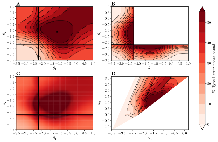
Figure 6: In plots A, B and C, the dark black lines indicate the boundary between the null space and the alternative space for each plotted parameter. A) The optimal Tilt-Bound as a function of $\theta_{1}$ and $\theta_{2}$ when $\theta_{3}=\theta_{4}=\theta_{critical}$. The open triangle and open star indicate the two peaks in Type I Error discussed in the text. B) The optimal Tilt-Bound as function of $\theta_{1}$ and $\theta_{2}$ with $\theta_{3}$ and $\theta_{4}$ fixed at the global maximum. Note that the white space in the figure indicates the parameter sets would fall in the alternative space for all arms, and therefore, the Tilt-Bound is not meaningful. C) For each value of $(\theta_{1},\theta_{2})$, the error surface shown is the worst-case Type I Error over $(\theta_{3},\theta_{4})$. D) For each $u_{1}=(\theta_{1}+\theta_{2}+\theta_{3}+\theta_{4})/4$ and $u_{2}=\max\limits_{i}(\theta_{i}-\theta_{0i})$, the error surface shown is the worst-case Type I Error over the remaining 2 dimensions

We consider $\theta_{i}\in[-3.5,1.0]$ for every $i$ and show four different meaningful portions of the resulting Tilt-Bound surface in Figure 6. The Tilt-Bound is as high as 60% for some parameter combinations, which is not surprising given that the design was not optimized to control the Type I Error. Nevertheless, the Tilt-Bound is well-controlled at the global null point where $\theta_{i}=\theta_{oi}$ for all arms. This is consistent with the results of [13], which calibrated these Bayesian analysis settings to ensure a low Type I Error at the global null point for a slightly more complicated version of this design.

The Tilt-Bound shows significant multi-modality with high error both near the null hypothesis boundary and at another peak further into the alternative space of $\theta_{1}$ and $\theta_{2}$. This multi-modality is due solely to the sharing effects (as the design is not adaptive). The open triangle and open star on Figure 6A indicate the peaks in the Tilt-Bound and correspond, respectively, to the “One Nugget” and “2 Null, 2 Alternative” simulations from [13]. The first peak (indicated by an open triangle in Figure 6A) occurs when the three variables, $\theta_{1}$, $\theta_{3}$ and $\theta_{4}$, are at their respective null hypothesis boundaries and the final variable, $\theta_{2}$ is deep into its alternative space. The sharing effect from the alternative-space variable pulls estimates of the three null-space variables across the rejection threshold, resulting in high Type I Error. Similarly, the second peak (indicated by an open star in Figure 6A) occurs when the un-plotted variables, $\theta_{3}$ and $\theta_{4}$, lie on their respective null hypothesis boundaries and the hierarchical model pulls their estimates towards the plotted alternative-space variables $\theta_{1}$ and $\theta_{2}$.

5 Calibrating the FWER of a Phase II/III Selection Design

In this section, we study a simplified Phase II/III selection design with a structure that was suggested to us by an FDA official. We wish to perform the calibration procedure as in Section 3.2 to obtain a level $\alpha$ test. Apart from calibration, the design is not otherwise optimized for performance. For general discussion on performing calibration of designs with adaptive stopping, see Appendix C.

This Phase II/III selection design has two stages: the first stage has 3 treatment arms and 1 control arm, and it may select a treatment for continuation against control in the second stage. Outcomes are assumed $\operatorname{Bern}(p_{i})$ for $i=0,\ldots,3$, with $i=0$ representing the control arm, and trial decisions are informed by the Bayesian hierarchical model described in Section 4 using data from all arms. At each of 3 interim analyses in the first stage, decision options include whether to stop for futility, to drop one or more poor-performing treatments, or to select a treatment for acceleration to the second stage. The second stage has one interim and one final analysis. The total number of patients across all arms and stages is at most 800 with at most 350 in any single arm. A full description is given in Appendix D.

We now restrict our attention to a bounded region of parameter space: the 4-dimensional cube $\Theta=[-1,1]^{4}$, where $\theta\in\Theta$ assigns $\operatorname*{logit}(p_{i})$ for each arm $i$ (so that $p_{i}$ ranges approx. [27%, 73%]). Each treatment arm for $i$ in $1,2,3$ has a null hypothesis denoted $H_{i}$, with null region given by

$$\Theta_{i}=\{\theta\in[-1,1]^{4}:\theta_{i}\leq\theta_{0}\}$$

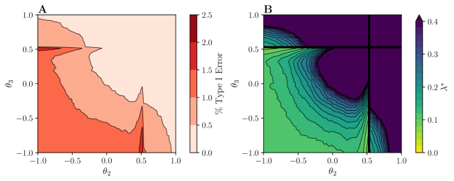
Figure 7: Calibration results of the Phase II/III design. Both plots slice the domain by fixing 2 parameters, $\theta_{0}=\theta_{1}=0.533$. Figure A shows the Tilt-Bound (Type I Error upper bound) profile for the selected threshold $\lambda=0.06253$. Figure B shows the critical value $\lambda^{*}$ separately for each tile such that its Tilt-Bound is 2.5%.

Calibration is only computationally tractable for this problem if we can use larger tiles for some (uninteresting) regions of space and small tiles for others. We adaptively use pilot simulations to select the geometry of tiles and number of simulations to perform. The smallest tiles have half-width $0.000488$ whereas the largest tiles have half-width $0.0625$. To grid the entire space at the density of the smallest tiles would require 281 trillion tiles. Instead, we used 38.6 million tiles. Tiles in regions of low Type I Error (FWER) use as few as 2048 simulations, while simulations in regions of high Type I Error use up to 524,288 simulations (Figure 8). In total, adaptive simulation reduces the total number of required simulations from $1.5\times 10^{20}$ to 960 billion for a total computational savings of approximately 160 million times. As noted above, without adaptivity, the solution here would be impossible even with the largest supercomputers available today. Instead, we are able to produce these results in 5 days with a single Nvidia V100 GPU.

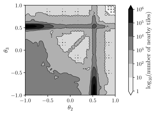
Figure 8: The number of tiles within a ball of radius 0.04 in the $\theta$ space. This shows how the adaptive algorithm assigns many more tiles to regions with high Type I Error. We show a slice of the domain where $\theta_{0}=\theta_{1}=0.533$.

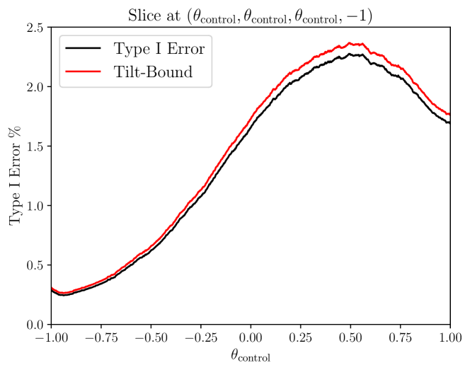
Figure 9: Type I Error estimates, with Tilt-bound from a separate simulation with fixed $\lambda=.06253$, focused on the 1-dimensional set where $\theta_{0}=\theta_{1}=\theta_{2}=\theta_{control}$ and $\theta_{3}=-1$. The worst case Type I Error appears when the trio of parameters is set to approximately 0.5.

We estimate using bootstrapping that at the critical point, the conservative bias due to estimation uncertainty accounts for an expected loss in Type I Error of about $0.16\%$ (out of a total target $2.5\%$); the amount of Type I Error spent on Tilt-Bound CSE from the simulation point to the edges of tiles is $0.06\%$. (We note that the latter quantity is not “purely slack” because the Type I Error at the simulation point is generally not the worst-case on its tile.)

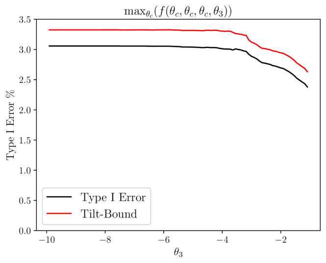
Figure 10: Worst-case Type I Error as a function of $\theta_{3}$, where the remaining $\theta_{i}$ are constrained equal to each other and then set to the value which maximizes Type I Error given $\theta_{3}$. Validation has been performed over this domain with $\lambda$ set to 0.06253; the Tilt-Bound is shown in red. In fact, it is possible to extend this graph from the leftmost point $\theta_{3}=-10$ $(p_{3}=0.000045)$ all the way to $\theta_{3}=-\infty$ $(p_{3}=0)$ at the cost of a small additional expansion of the bound by about 0.3% (not shown). This is possible because the sequence of distributions as $\theta_{3}\to-\infty$ converges in total variation, and if $\theta_{i}<-10$, the arm is overwhelmingly likely to dropped before it generates any successes whatsoever. From the left end-point $\theta_{3}=-10$, since we can safely assume that this arm would be dropped after observing zero successes out of $n_{3}=50$ patients, the resulting bound would be a penalty of $<0.3\%$ added to the Type I Error at the leftmost point of the figure.

The Tilt-Bound profile of the calibrated design is presented in Figure 7. The maximum of the Tilt-Bound occurs at the tile centered at $\theta=(0.4925,0.4925,\\ 0.4925,-1.0)$. Surprisingly, the worst Type I Error point does not occur at the global null (where all treatments perform equally to control), but rather when one treatment performs poorly. It appears this “rogue arm” paradoxically increases the chance that other treatments are incorrectly rejected, because the observed heterogeneity causes a reduction in Bayesian borrowing. Unlike the design studied in Section 4, borrowing effects from highly successful arms do not cause Type I Error inflation. The Type I Error profile is non-monotonic with respect to $\theta_{i}$ and maximized away from the global null.

We remark that with the standard method of simply performing simulations at each grid point (i.e. without CSE), it would be difficult to establish worst-case control. Even after correctly guessing at the $(\theta,\theta,\theta,-1)$ form of the worst-case point, one would still need a 1-dimensional search of Type I Error over $\theta$ (such as Figure 9). In contrast, the “proof-by-simulation” approach, establishes Type I Error control over the region of interest unambiguously.

However, CSE guarantees do not necessarily extend outside of the region of focus. If $\theta_{3}$ is permitted to drop below $-1$, as shown in Figure 10 the worst-case Type I Error rises above 2.5% and asymptotes at approximately 3.1%. If a 2.5% guarantee were desired for this area, then the initial domain $\Theta$ should have been extended to a wider region at the outset of calibration (although at an additional computational cost). Interestingly, it is technically possible to give a bound which extends Figure 10 to the left all the way to $\theta_{3}=-\infty$ $(p_{3}=0)$ at the cost of a small additional penalty. See description of Figure 10.

6 Guide to Supplementary Information

In Appendix A, we formalize CSE with the Tilt-Bound from a mathematical point of view. We develop a main theorem that shows CSE can be applied to general metrics including Type I Error, power, FWER, FDR, and the bias of a bounded estimator. We also show that CSE can be used on 3 classes of problems: exponential families, canonical generalized linear models, and a simple non-parametric regression model with parametrized (Gaussian) noise.

In Appendix B, we formalize CSE calibration and prove that it achieves Type I Error control.

In Appendix C, we discuss further details for applying CSE to adaptive trials with a pre-specified design plan, administrative censoring, and/or latent variables. We do not discuss unplanned design modifications, arm additions, or platform trials. These topics are covered in Chapter 5 of [12], and will be a topic of future work.

In Appendix D, the design in Section 5 is fully described.

7 Discussion

Proof-by-simulation is a powerful and robust methodology. It places minimal constraints on the structure of the test and sampling decisions, and therefore can successfully validate procedures that defy classical analysis. Continuous Simulation Extension (CSE) enhances simulation-gridding with guarantees, providing an objective standard and removing doubts about potentially missing areas of the null hypothesis space or selective presentation of results.

A further practical advantage of CSE is that it analyzes the design as represented in code. Thus, CSE offers designers a “free pass” to make approximations in their statistical analyses, and defuses theoretical uncertainties such as convergence of MCMC samplers. In fact, even if the design contains an incorrect implementation or subtle software bug, the guarantees from CSE are technically valid as long as the real-world implementation precisely matches the code.

To ensure CSE’s conservatism is kept small, the number of simulations required grows with the dimension of the parameter space. Our examples demonstrate that up to 4 unknown parameters can be handled using trillions of simulations. We anticipate that large-scale computing will only become easier with time; in addition, our framework can be made more efficient with improvements to tile geometry, better adaptive gridding, and extensions to importance sampling. Thus, the set of compatible applications will grow.

For regulatory applications, a subjective issue remains: how to justify the modeling family over which CSE will provide its guarantees? The history of previously accepted models is important here, but outside the scope of this paper. Yet it bears mentioning that CSE should be easier for regulators to accept than parametric regression methods. To perform inference on a parametrized regression model, such as a confidence interval on the parameters of a logistic regression, requires estimability of the model as well as the relevance of the model class for inference. CSE relies only on the relevance; therefore even in cases where a parametric regression model is too uncertain or unstable to use, CSE can still be justified.

If there are multiple candidates for the distributional family, additional evidence of robustness can be given by performing CSE for each of them, or by embedding the models in a larger family. We are in the initial stages of extending CSE to nonparametric and semi-parametric models (see Appendix A Example 3), although we are as yet unsure of its computational feasibility.

We also remark that even if distributional assumptions fail, Gaussian process limiting behavior is powerful and in some cases may carry the day asymptotically. For example: consider applying CSE to a model assuming $\Gamma(\alpha,\beta)$ outcomes where $(\alpha,\beta)$ are unknown. If the data are not truly $\Gamma$-distributed, the test statistic may still have an asymptotic $\operatorname{\mathcal{N}}(\mu,\sigma^{2})$ distribution. Furthermore, each $\Gamma(\alpha,\beta)$ input may also map approximately to some asymptotic-limiting $\operatorname{\mathcal{N}}(\mu,\sigma^{2})$ for the test statistic. In this case, using CSE to control Type I Error over a wide range range of $(\alpha,\beta)$ would imply asymptotic control over the range of possible distributions which converge similarly. Assuming a sufficiently continuous design logic and correspondence of the relevant null hypothesis spaces, one could derive a general version of this argument for adaptive tests using asymptotic Brownian limits.

The rigorous foundation laid by proof-by-simulation tools can support new innovations in design optimization. For example, CSE could be a component of a tool that would tighten or level out the Type I Error surface of a design. CSE could also be used as an “inner loop” to a design optimization protocol, where CSE is used at each iteration to either ensure that the current version of the design is valid, or to identify and quantify constraint violations. More speculatively, this framework could even be used to validate or calibrate “black-box” design protocols, like using a neural network to determine randomization probabilities or stopping decisions as a function of the sufficient statistics.

Ultimately, our hope is that these proof-by-simulation techniques can speed up innovation cycles. Properly implemented, we believe proof-by-simulation can reduce the human capital cost of parsing and validating new trial designs, improve regulatory consistency by enabling rigorous satisfaction of objective standards, and offer innovators in design a rapid alternative to peer review for establishing formal claims. We invite statisticians and regulators to explore our open-source code repository at [1] and consider its use as the next generation of statistical methodology is being developed.

8 Acknowledgements

We thank Alex Constantino and Gary Mulder for significant volunteer contributions to our software. Thanks also to Daniel Kang, Art Owen, Narasimhan Balasubramanian, and various regulators and biostatisticians for help and advice. This work was supported by ACX Grants and FTX Future Fund.

Appendix A Continuous Simulation Extension

In this section, we derive several main theorems for continuous simulation extension (CSE). Application of the main theorems can convert upper bounds at points into upper bounds over continuous space. We apply the main results to Type I Error in Section A.3, FDR in Section A.4, and bias of bounded estimators in Section A.5. The upper bound in its abstract form holds with minimal assumptions on the simulation outcome distribution, and can be extended to log-concave distributions; under exponential family assumptions, it has a convenient analytical form which we derive in Section X.

A.1 Grid Space and Null Hypothesis Space

We discuss the notion of a grid space. As described in Section 3, we must create a grid of parameters in the null hypothesis space. As an example, for a Bernoulli outcome model with three arms, one could take $\Theta$ to be a compact subset of $\mathbb{R}^{3}$ where each $\theta\in\Theta$ has components that correspond to the natural parameters of each arm, $\theta_{i}:=\log(p_{i}/(1-p_{i})),$ where $p_{i}$ is the probability of success in arm $i$.

Let $\Theta$ denote a compact grid space. Suppose there exists a cover of $\Theta$, $\{H_{i}\}_{i=1}^{I}$, such that the interiors of $H_{i}$ are disjoint. We call this cover $\{H_{i}\}_{i=1}^{I}$ a collection of tiles for $\Theta$. We say $\{H_{i}\}_{i=1}^{I},\{\theta_{i}\}_{i=1}^{I}$ is a platten if $\{H_{i}\}_{i=1}^{I}$ are tiles and $\{\theta_{i}\}_{i=1}^{I}$ are any set of arbitrary points in $\Theta$, with shared indexing $i$ associating each tile with one point.

A.2 Main Theorems

Theorem 1 is a general theorem to provide an upper bound of an expectation of a $[0,1]$-valued function under a parameter $\theta$ around a fixed point $\theta_{0}$.

Theorem 1 (Tilt-Bound).

Let $\{P_{\theta}:\theta\in\Theta\}$ denote a family of distributions with density

$$p_{\theta}(x)=\exp\left[g_{\theta}(x)-A(\theta)\right]$$ (12)

for some functions $g_{\theta}(x):=g(\theta,x)$ and $A(\theta)$ such that $\int p_{\theta}(x)d\mu(x)=1$ for some base measure $\mu$. Fix an “origin point” $\theta$ and “destination point” $\theta+v$. Denote

$$\Delta_{\theta}(v,x) :=g_{\theta+v}(x)-g_{\theta}(x)$$ (13)

$$\psi(\theta,v,q) :=\log\mathbb{E}_{\theta}\left[e^{q\Delta_{\theta}(v,X)}\right]$$ (14)

Suppose $F:\mathbb{R}\to[0,1]$ is a measurable function and $f(\theta):=\mathbb{E}_{\theta}\left[F(X)\right]$ where $X\sim P_{\theta}$. Then, for any $\theta_{0}\in\Theta$, $v\in\Theta-\theta_{0}$, and $q\geq 1$,

$$f(\theta_{0}+v) \leq U(\theta_{0},v,q,f(\theta_{0}))$$ (15)

where

$$U(\theta_{0},v,q,a) :=a^{1-\frac{1}{q}}\exp\left[\frac{\psi(\theta_{0},v,q)}{q}-\psi(\theta_{0},v,1)\right]$$ (16)

The bound (16) is called the Tilt-Bound.

Proof.

Fix any $q\geq 1$ and define its Hölder conjugate $p:=\left(1-q^{-1}\right)^{-1}$, with the convention that $p=\infty$ if $q=1$. Define

$$\ell_{\theta}(x):=\log p_{\theta}(x)=g_{\theta}(x)-A(\theta)$$

Fix any $\theta_{0}\in\Theta$. Then, for any $\theta\in\Theta$,

$$f(\theta) =\mathbb{E}_{\theta}\left[F(X)\right]=\mathbb{E}_{\theta_{0}}\left[F(X)e^{\ell_{\theta}(X)-\ell_{\theta_{0}}(X)}\right]$$

$$\leq\left\lVert F(X)\right\rVert_{L^{p}(P_{\theta_{0}})}\left\lVert e^{\ell_{\theta}(X)-\ell_{\theta_{0}}(X)}\right\rVert_{L^{q}(P_{\theta_{0}})}$$

$$=\left\lVert F(X)\right\rVert_{L^{p}(P_{\theta_{0}})}\left\lVert e^{g_{\theta}(X)-g_{\theta_{0}}(X)}\right\rVert_{L^{q}(P_{\theta_{0}})}e^{-\left(A(\theta)-A(\theta_{0})\right)}$$

$$\leq f(\theta_{0})^{\frac{1}{p}}\left(\mathbb{E}_{\theta_{0}}\left[e^{q\left(g_{\theta}(X)-g_{\theta_{0}}(X)\right)}\right]\right)^{\frac{1}{q}}e^{-\left(A(\theta)-A(\theta_{0})\right)}$$

Noting that

$$\psi(\theta_{0},v,1)\equiv A(\theta_{0}+v)-A(\theta_{0})$$

we have that for any $v\in\Theta-\theta_{0}$,

$$f(\theta_{0}+v) \leq f(\theta_{0})^{\frac{1}{p}}\exp\left[\frac{\psi(\theta_{0},v,q)}{q}-\psi(\theta_{0},v,1)\right]$$

∎

Remark 1.

In Theorem 1, the Tilt-Bound may be infinite, however, (16) still holds formally.

Remark 2.

The Tilt-Bound as a function of $v$ may be well-defined even outside of $\Theta-\theta_{0}$.

Note that the Tilt-Bound holds generally with minimal assumptions. However, it is defined for a fixed choice of $v$. In practice, we consider a bounded subset $H\subseteq\Theta-\theta_{0}$ and wish to compute a bound for $\sup\limits_{v\in H}f(\theta_{0}+v)$. That is, we would like to compute $\sup\limits_{v\in H}U(\theta_{0},v,q,f(\theta_{0}))$. If one imposes more structure on the distribution $P_{\theta}$, we prove in Lemma 2 that the Tilt-bound is quasi-convex as a function of $v$. Consequently, if $H$ is a polytope, the maximum is attained at one of the vertices.

Lemma 2 (Quasi-convexity in $v$ of the Tilt-Bound).

Consider the setting of Theorem 1. Fix any $\theta_{0}\in\Theta$. Suppose that $\Delta(v,x)\equiv\Delta_{\theta_{0}}(v,x)$ in (13) is linear in $v$, i.e. $\Delta(v,x)=W(x)^{\top}v$ for some vector $W(x)\in\mathbb{R}^{d}$. Then, the Tilt-Bound (16) is quasi-convex as a function of $v$.

Proof.

Fix any $\theta_{0}\in\Theta$.

For every $q\geq 1$, define $\mathcal{D}_{q}:=\{v\in\mathbb{R}^{d}:\psi(\theta_{0},v,q)<\infty\}$. By Lemma 4, $\mathcal{D}_{q}=\{v:|\varphi_{q}(v)|<\infty\}$. Convexity of $\mathcal{D}_{q}$ is also shown in Lemma 4. To establish quasi-convexity of the Tilt-Bound (16) as a function of $v$, it therefore suffices to show that $\varphi_{q}(v)$ is quasi-convex along all 1-dimensional line segments contained in $\mathcal{D}_{q}$. Let $a$, $b$ be any two points in $\mathcal{D}_{q}$, and $\overline{ab}$ the line segment joining them. We may consider the directional unit vector $u=\frac{b-a}{\|b-a\|}$, extend the line segment to make a full line $\overleftrightarrow{ab}$, and then drop a perpendicular vector $v_{0}$ which measures the distance from the origin to $\overleftrightarrow{ab}$. Hence, it suffices, without loss of generality, to show that $h\mapsto\varphi_{q}(v_{0}+hu)$ is quasi-convex for all vectors $v_{0}$ and $u$ such that $u\perp v_{0}$ and $h\in\mathcal{D}_{q,v_{0},u}:=\{t\in\mathbb{R}:v_{0}+tu\in\mathcal{D}_{q}\}$. Note that $\mathcal{D}_{q,v_{0},u}$ is an interval by convexity of $\mathcal{D}_{q}$.

Without loss of generality, fix any such $v_{0}$ and $u$. Denote $\mathcal{D}\equiv\mathcal{D}_{q,v_{0},u}$ for notational ease. Define $\tilde{\varphi}_{q}(h):=\varphi_{q}(v_{0}+hu)$. We wish to show that $\tilde{\varphi}_{q}$ is quasi-convex on $\mathcal{D}$. Lemma 3 shows that $\frac{\partial}{\partial h}\tilde{\varphi}_{q}(h)\geq 0$ for all $h\in\mathcal{D}\cap(0,\infty)$, which shows that $\tilde{\varphi}_{q}(h)$ is non-decreasing for $h\in\mathcal{D}\cap(0,\infty)$. Note that since $\Delta(\cdot,X)$ is linear, we have by standard exponential family that $v\mapsto\psi(\theta_{0},v,q)$ is continuous on $\mathcal{D}_{q}$. Then, by Lemma 4, $\varphi_{q}$ is continuous on $\mathcal{D}_{q}$, so that $\tilde{\varphi}_{q}$ is non-decreasing on $\mathcal{D}\cap[0,\infty)$. Therefore, applying the same logic for $-u$, $\tilde{\varphi}_{q}$ must either be monotone on $\mathcal{D}$ or decreasing from the left end-point of $\mathcal{D}$ to $0$ then increasing to the right end-point of $\mathcal{D}$. Thus, $\tilde{\varphi}_{q}$ is quasi-convex along the segment $\mathcal{D}$, as needed. ∎

Lemma 3 (Monotonicity of $\tilde{\varphi}_{q}$).

Consider the setting of Lemma 2, including the definitions of $u,v_{0},h,\mathcal{D}$ in the proof. For all $h\in\mathcal{D}\cap(0,\infty)$, $\frac{\partial}{\partial h}\tilde{\varphi}_{q}(h)\geq 0$.

Proof.

Begin with the expression from the chain rule:

$$\frac{\partial}{\partial h}\tilde{\varphi}_{q}(h) =\nabla\varphi_{q}(v_{0}+hu)^{\top}u$$

$$\nabla\varphi_{q}(v) =\frac{\nabla_{v}\psi(\theta_{0},v,q)}{q}-\nabla_{v}\psi(\theta_{0},v,1)$$

Since $h>0$, letting $u_{h}:=hu$, we may equivalently show that

$$h\frac{\partial}{\partial h}\tilde{\varphi}_{q}(h)=\nabla\varphi_{q}(v_{0}+u_{h})^{\top}u_{h}\geq 0$$

To establish the above, by an integration argument, it suffices to show that

$$\frac{\partial}{\partial t}\left(\frac{\nabla_{v}\psi(\theta_{0},v_{0}+u_{h},t)^{\top}u_{h}}{t}\right)\geq 0$$

for $t\in[1,q]$. Note that all terms are well-defined for any $t\in[1,q]$ since

$$v_{0}+u_{h}\in\mathcal{D}_{q}=\bigcap\limits_{t\in[1,q]}\mathcal{D}_{t}$$

by Lemma 4. By integrating, we then have that

$$h\frac{\partial}{\partial h}\tilde{\varphi}_{q}(h) =\int_{1}^{q}\frac{\partial}{\partial t}\left(\frac{\nabla_{v}\psi(\theta_{0},v_{0}+u_{h},t)^{\top}u_{h}}{t}\right)dt\geq 0$$

For any $v\in\mathbb{R}^{d}$, define a family of distributions

$$\mathcal{Q}_{v}:=\{Q_{t,v}:t\geq 1,\,\psi(\theta_{0},v,t)<\infty\}$$

where $Q_{t,v}$ is given by

$$dQ_{t,v}(x) :=\exp\left[t\Delta(v,x)-\psi(\theta_{0},v,t)\right]dP_{\theta_{0}}(x)$$

Using the definition of $\psi$ and $Q_{t,v}$, we have that

$$\nabla_{v}\psi(\theta_{0},v,t) =te^{-\psi(\theta_{0},v,t)}\mathbb{E}_{\theta_{0}}\left[\nabla_{v}\Delta(v,X)e^{t\Delta(v,X)}\right]$$

$$=t\mathbb{E}_{Q_{t,v}}\left[\nabla_{v}\Delta(v,X)\right]$$

Hence, for any $t\in[1,q]$,

$$\frac{\nabla_{v}\psi(\theta_{0},v_{0}+u_{h},t)^{\top}u_{h}}{t} =\mathbb{E}_{Q_{t,v_{0}+u_{h}}}\left[\nabla_{v}\Delta(v_{0}+u_{h},X)^{\top}u_{h}\right]$$ (17)

Note that $Q_{t,v}$ forms an exponential family with natural parameter $t$, sufficient statistic $\Delta(v,x)$, and log-partition function $\psi(\theta_{0},v,t)$ with base measure $P_{\theta_{0}}$. By standard results for exponential family, the derivative of (17) with respect to $t$ is

$$\operatorname{Cov}_{Q_{t,v_{0}+u_{h}}}\left(\nabla_{v}\Delta(v_{0}+u_{h},X)^{\top}u_{h},\;\Delta(v_{0}+u_{h},X)\right)$$

$$\qquad=u_{h}^{\top}\left[\operatorname{Var}_{Q_{t,v_{0}+u_{h}}}W(X)\right](v_{0}+u_{h})$$

Let $P_{0}$ denote the projection matrix onto $\text{span}(v_{0})^{\perp}$. Then, since $u_{h}^{T}\left(I-P_{0}\right)=v^{T}P_{0}=\vec{0}$, we have

$$u_{h}^{\top}\left[\operatorname{Var}_{Q_{t,v_{0}+u_{h}}}W(X)\right]\,(v_{0}+u_{h})$$

$$\qquad=(v_{0}+u_{h})^{\top}P_{0}\left[\operatorname{Var}_{Q_{t,v_{0}+u_{h}}}W(X)\right]\,(v_{0}+u_{h})$$ (18)

Since $P_{0}$ and $\operatorname{Var}_{Q_{t,v_{0}+u_{h}}}W(X)$ are both positive semi-definite, their product must have all non-negative eigenvalues. Hence, the right-side of (18) is non-negative. This proves that $\frac{\partial}{\partial h}\tilde{\varphi}_{q}(h)\geq 0$ on $\mathcal{D}\cap(0,\infty)$.

∎

Lemma 4 (Basic Properties of $\mathcal{D}_{q}$ and $\varphi_{q}$).

Consider the setting of Theorem 1. Fix any $\theta_{0}\in\Theta$. Define $\mathcal{D}_{q}$ and $\varphi_{q}$ as in Lemma 2. Define $\mathcal{I}_{v}:=\{q\geq 1:\psi(\theta_{0},v,q)<\infty\}$. Let $q_{1}$, $q_{2}$ be any pair such that $1\leq q_{1}<q_{2}$. Then, the following statements hold:

1. $\mathcal{D}_{q_{1}}\supseteq\mathcal{D}_{q_{2}}$.

2. Assume $v\mapsto\Delta_{\theta_{0}}(v,x)$ is linear, then $\mathcal{D}_{q}$ is convex.

3. $\mathcal{D}_{q}=\{v:0\leq\varphi_{q}(v)<\infty\}$.

4. Assume $v\mapsto\psi(\theta_{0},v,q)$ is continuous on $\mathcal{D}_{q}$, then $v\mapsto\varphi_{q}(v)$ is continuous on $\mathcal{D}_{q}$.

5. $\mathcal{I}_{v}$ is convex and $q\mapsto\psi(\theta_{0},v,q)$ is convex on $\mathcal{I}_{v}$. It is strictly convex if $\Delta_{\theta_{0}}(v,X)$ is not constant $P_{\theta_{0}}$-a.s.

Proof.

If $v\in\mathcal{D}_{q_{2}}$, then $\psi(\theta_{0},v,q_{2})<\infty$. By Jensen’s Inequality,

$$\left\lVert e^{\Delta(v,X)}\right\rVert_{L^{q_{1}}(P_{\theta_{0}})} \leq\left\lVert e^{\Delta(v,X)}\right\rVert_{L^{q_{2}}(P_{\theta_{0}})}$$

$$\implies\frac{1}{q_{2}}\psi(\theta_{0},v,q_{1}) \leq\frac{1}{q_{2}}\psi(\theta_{0},v,q_{2})<\infty$$ (19)

Thus, we have 1.

Without loss of generality, now assume that $\mathcal{D}_{q}$ is non-empty. For any $v_{1},v_{2}$ and any $\lambda\in(0,1)$,

$$\mathbb{E}_{\theta_{0}}\left[e^{q\Delta_{\theta_{0}}(\lambda v_{1}+(1-\lambda)v_{2},X)}\right] \leq\mathbb{E}_{\theta_{0}}\left[e^{q\Delta_{\theta_{0}}(v_{1},X)}\right]^{\lambda}\mathbb{E}_{\theta_{0}}\left[e^{q\Delta_{\theta_{0}}(v_{2},X)}\right]^{1-\lambda}$$

by Hölder’s Inequality and linearity of $\Delta_{\theta_{0}}(\cdot,X)$. Taking $\log$ on both sides,

$$\psi(\theta_{0},\lambda v_{1}+(1-\lambda)v_{2},q) \leq\lambda\psi(\theta_{0},v_{1},q)+(1-\lambda)\psi(\theta_{0},v_{2},q)<\infty$$

Thus, $\lambda v_{1}+(1-\lambda)v_{2}\in\mathcal{D}_{q}$. This proves 2.

Next, we consider the function:

$$\varphi_{q}(v) :=\frac{\psi(\theta_{0},v,q)}{q}-\psi(\theta_{0},v,1)$$

as in Lemma 2. Note that $\psi(\theta_{0},v,1)$ cannot be $-\infty$, because $P_{\theta+v}$ is a probability measure absolutely continuous to $P_{\theta}$. Also, $\mathcal{D}_{1}\supseteq\mathcal{D}_{q}$. Therefore, for $v\in\mathcal{D}_{q}$, we must have $\varphi_{1}(v)=0$. Further, (19) shows that $q\mapsto\frac{\psi(\theta_{0},v,q)}{q}$ is non-decreasing. Thus,

$$\mathcal{D}_{q}:=\{v:\left|\varphi_{q}(v)\right|<\infty\}=\{v:0\leq\varphi_{q}(v)<\infty\}$$

Thus, this proves 3.

Next, since $v\mapsto\psi(\theta_{0},v,q)$ is continuous on $\mathcal{D}_{q}$ and $\mathcal{D}_{q}\subseteq\mathcal{D}_{1}$, $\varphi_{q}(v)$ is continuous on $\mathcal{D}_{q}$. This proves 4.

Finally, we show that $\mathcal{I}_{v}$ is convex. For notational ease, let $Z:=\Delta_{\theta_{0}}(v,X)$. For any $q_{1}\neq q_{2}\in\mathcal{I}_{v}$ and $\lambda\in(0,1)$, we apply Hölder’s Inequality to get that

$$\mathbb{E}_{\theta_{0}}\left[e^{\left(\lambda q_{1}+(1-\lambda)q_{2}\right)Z}\right] \leq\mathbb{E}_{\theta_{0}}\left[e^{q_{1}Z}\right]^{\lambda}\mathbb{E}_{\theta_{0}}\left[e^{q_{2}Z}\right]^{1-\lambda}$$

Taking $\log$ on both sides,

$$\psi(\theta_{0},v,\lambda q_{1}+(1-\lambda)q_{2}) \leq\lambda\psi(\theta_{0},v,q_{1})+(1-\lambda)\psi(\theta_{0},v,q_{2})<\infty$$

Hence, $\lambda q_{1}+(1-\lambda)q_{2}\in\mathcal{I}_{v}$. This proves that $\mathcal{I}_{v}$ is convex and $q\mapsto\psi(\theta_{0},v,q)$ is convex on $\mathcal{I}_{v}$. Note that Hölder’s Inequality is an equality if and only if there exists $\alpha,\beta\geq 0$ not both zero such that

$$\alpha e^{q_{1}Z}=\beta e^{q_{2}Z}$$

This can only occur if $q_{1}=q_{2}$ or $Z$ is constant $P_{\theta_{0}}$-a.s. Hence, if $Z$ is not constant $P_{\theta_{0}}$-a.s., $q\mapsto\psi(\theta_{0},v,q)$ is strictly convex on $\mathcal{I}_{v}$. ∎

Remark 3.

Lemma 2 shows that on a polytope $H\subseteq\mathbb{R}^{d}$, the Tilt-Bound attains its maximum at a vertex. Therefore, the quasi-convexity simplifies the computation of

$$\sup\limits_{v\in H}U(\theta_{0},v,q,f(\theta_{0}))$$

to computing the maximum bound on a (finite) set of vertices .

Remark 4.

For an arbitrary bounded set $H\subseteq\Theta-\theta_{0}$, we may also construct a conservative upper bound. Define $\pi_{i}(H):=\{v_{i}:v\in H\}\subseteq\mathbb{R}$ to be the projection of $H$ onto the $i$th coordinate. Let $l_{i}(H):=\inf\pi_{i}(H)$ and $u_{i}(H):=\sup\pi_{i}(H)$ be the lower and upper end-points of $\pi_{i}(H)$. Finally, define $R(H):=\prod\limits_{i=1}^{d}\{l_{i}(H),u_{i}(H)\}$ to be set of vertices of a rectangle enclosing $H$. Note that these are well-defined since $H$ is bounded. Theorem 1 and Lemma 2 show that for any $q\geq 1$,

$$\sup\limits_{v\in H}f(\theta_{0}+v) \leq\sup\limits_{v\in H}U(\theta_{0},v,q,f(\theta_{0}))$$

$$\leq\sup\limits_{v\in\prod\limits_{i=1}^{d}\pi_{i}(H)}U(\theta_{0},v,q,f(\theta_{0}))$$

$$=\max\limits_{v\in R(H)}U(\theta_{0},v,q,f(\theta_{0}))$$

Lemma 2 requires the crucial assumption that $\Delta(v,x)$ is linear in $v$. Fortunately, a wide range of distributions satisfy the linearity condition. We list several examples:

Example 1 (Exponential Family).

Suppose $\{P_{\theta}:\theta\in\Theta\}$ is an exponential family with natural parameter $\theta$ so that the density is of the form

$$p_{\theta}(x) =\exp\left[g_{\theta}(x)-A(\theta)\right]$$

where $g_{\theta}(x)=T(x)^{\top}\theta$. Then, for any $\theta_{0}\in\Theta$,

$$\Delta(v,x)=g_{\theta_{0}+v}(x)-g_{\theta_{0}}(x)=T(x)^{\top}v$$

Since $\Delta$ is linear in $v$, we have the conclusion of Lemma 2.

Example 2 (Canonical Generalized Linear Model (GLM)).

Under the canonial GLM framework, we model each response $y_{i}$ as exponential family where the natural parameter is parameterized as $x_{i}^{\top}\theta$ (fixed $x_{i}$’s). Hence, letting $y\in\mathbb{R}^{n}$ be the vector of responses and $X\in\mathbb{R}^{n\times d}$ denote the matrix of covariates with each row as $x_{i}^{\top}$, the density of $y$ is of the form

$$p_{\theta}(y) =\exp\left[g_{\theta}(y)-A(\theta)\right]$$

with $g_{\theta}(y):=y^{\top}X\theta$. Hence, for every fixed $\theta_{0}\in\Theta$,

$$\Delta(v,y) =g_{\theta_{0}+v}(y)-g_{\theta_{0}}(y)=y^{\top}Xv$$

Since $\Delta$ is linear in $v$, we have the conclusion of Lemma 2.

While the Tilt-Bound is posed with parametric data, non-parametric analysis sometimes holds. Example 3 shows an example of applying the Tilt-Bound for testing a non-parametric model with Gaussian additive noise.

Example 3 (Non-parametric Model with Gaussian Noise).

Assume a simple non-parametric model for outcomes $Y=\{y_{i}\}$ conditioned on a (1-dimensional) covariate $X=\{x_{i}\}$ for $i\in 1,\ldots,n$:

$$y_{i} =g(x_{i})+\epsilon_{i}\quad$$

$$\epsilon_{i} \sim\operatorname{\mathcal{N}}(0,1)$$

Consider a test of the form $F(y):=\mathbbm{1}\left(y\in S\right)$ for some set $S$. We assume the regression function $g\in G$ is not known. Our goal is to bound over $G$ the Type I Error conditioned on the covariate vector, i.e. a bound on $f_{X}(g):=\mathbb{E}_{g}\left[F(Y)|X\right]$. We may define the metric

$$d_{L^{2}_{X}}(a,b):=\left(\sum\limits_{i=1}^{n}\left[a(x_{i})-b(x_{i})\right]^{2}\right)^{\frac{1}{2}}$$

and aim to derive a bound valid within a $L^{2}_{X}$ neighborhood of some function $h$. We apply the Tilt-Bound directly. Conditional on $X$, the distribution of $Y$ is an $n$-dimensional Gaussian, hence an $n$-dimensional exponential family. The Tilt-Bound evaluates to

$$f_{X}(g) \leq f_{X}(h)^{1-\frac{1}{q}}\exp\left[\frac{q-1}{2}\left\lVert h-g\right\rVert^{2}_{L^{2}_{X}}\right]$$ (20)

Conveniently, for $g$ in the $L^{2}_{X}$ ball of $h$ of radius $r$, $B_{L^{2}_{X}}(h,r)$, the worst case of this bound occurs at all points on the boundary of $B_{L^{2}_{X}}(h,r)$. As a result, CSE can be applied to bound $f_{X}(g)$ over a covering of $G$ with an $\epsilon$-net in $L^{2}_{X}$, and using (20) to bound each $\epsilon$-ball of the covering.

We are now prepared to ask: how to optimize the maximum bound

$$\sup\limits_{v\in H}U(\theta_{0},v,q,f(\theta_{0}))$$

with respect to $q$ to achieve the tightest bound? Lemma 5 shows that optimizing for $q$ is a quasi-convex program.

Lemma 5 (Quasi-convexity in $q$ of the Tilt-Bound).

Let $\{P_{\theta}:\theta\in\Theta\}$ be as in (12) and $U$ be as in (16). Fix any $\theta_{0}\in\Theta\subseteq\mathbb{R}^{d}$, a set $S\subseteq\mathbb{R}^{d}$, and $a\geq 0$. Assume that for all $v\in S$, $\Delta(v,X)$ in (13) is not constant $P_{\theta_{0}}$-a.s. Then, there exists a global minimizer $q^{*}\equiv q^{*}(\theta_{0},v,a)\in[1,\infty]$ of the function $q\mapsto\sup\limits_{v\in S}U(\theta_{0},v,q,a)$. Moreover, it is unique if $a>0$, $S$ is finite, and $q\mapsto\sup\limits_{v\in S}U(\theta_{0},v,q,a)$ is not identically infinite.

Proof.

Fix $\theta_{0}\in\Theta$, a set $S\subseteq\mathbb{R}^{d}$, and $a\geq 0$. Without loss of generality, assume $a>0$. If $a=0$, we may simply set $q^{*}\equiv\infty$. Note that any $q\geq 1$ achieves the minimum, so the minimizer is not unique.

Let $\mathcal{I}_{v}$ be as in Lemma 4. Define $\mathcal{I}:=\bigcap\limits_{v\in S}\mathcal{I}_{v}$. By Lemma 4, $\mathcal{I}$ is convex as well. It suffices to minimize

$$q\mapsto\sup\limits_{v\in S}U(\theta_{0},v,q,a)$$

on $\mathcal{I}$ since it is infinite on $\mathcal{I}^{c}$. Without loss of generality, assume that $\mathcal{I}$ is non-empty, or equivalently, $q\mapsto\sup\limits_{v\in S}U(\theta_{0},v,q,a)$ is not identically infinite. Otherwise, we may set $q^{*}\equiv\infty$ and the minimizer is not unique.

We show that $q\mapsto\sup\limits_{v\in S}U(\theta_{0},v,q,a)$ is quasi-convex on $\mathcal{I}$ and is strict if $S$ is finite. Note that

$$\sup\limits_{v\in S}U(\theta_{0},v,q,a) =a\cdot\exp\left[\sup\limits_{v\in S}\left[\frac{\psi(\theta_{0},v,q)-\log(a)}{q}-\psi(\theta_{0},v,1)\right]\right]$$

To establish the desired claim, we show that $\tilde{\psi}(q)$ is (strictly, if finite $S$) quasi-convex on $\mathcal{I}$ where

$$\tilde{\psi}(q) :=\sup\limits_{v\in S}\tilde{\psi}_{v}(q)$$

$$\tilde{\psi}_{v}(q) :=\frac{\psi(\theta_{0},v,q)-\log(a)}{q}-\psi(\theta_{0},v,1)$$

It suffices to show that $q\mapsto\tilde{\psi}_{v}(q)$ is strictly quasi-convex on $\mathcal{I}_{v}$ for every $v\in S$. Note that $\tilde{\psi}_{v}(q)=\frac{f_{1}(q)}{f_{2}(q)}$ where

$$f_{1}(q) :=\psi(\theta_{0},v,q)-\log(a)-q\psi(\theta_{0},v,1)$$

$$f_{2}(q) :=q$$

Lemma 4 shows that $q\mapsto\psi(\theta_{0},v,q)$ is strictly convex on $\mathcal{I}_{v}$, which directly shows the same for $f_{1}(q)$. Then, Lemma 6 shows that $\tilde{\psi}_{v}(q)$ is strictly quasi-convex.

Finally, since $\tilde{\psi}$ is (strictly, if finite $S$) quasi-convex on $\mathcal{I}$, we have the following quasi-convex program:

$$\operatorname*{minimize\;}\limits_{q}\tilde{\psi}(q)$$

$$\operatorname{subject\;to}\quad q\in\mathcal{I}$$

This proves the existence (and uniqueness for finite $S$) of a global minimizer $q^{*}\in\mathcal{I}\subseteq[1,\infty]$. ∎

Combining Lemma 2 and Lemma 5, we may obtain the tightest bound

$$\inf\limits_{q\geq 1}\sup\limits_{v\in H}U(\theta_{0},v,q,f(\theta_{0}))$$

by solving a simple quasi-convex program.

Remark 5.

If one were to use a non-optimal value of $q$ instead of solving the optimization in Lemma 5, the bounding inequality is still valid, but it may be undesirably loose.

Lemma 6.

Let $f(x)=\frac{f_{1}(x)}{f_{2}(x)}$ where $f_{1}:C\mapsto\mathbb{R}$ and $f_{2}:C\mapsto(0,\infty)$ for some convex set $C$. If $f_{1}$ is strictly convex and $f_{2}$ concave, then $f$ is strictly quasi-convex.

Proof.

Fix any $x\neq y\in C$ and $\lambda\in(0,1)$. Then,

$$f(\lambda x+(1-\lambda)y) <\frac{\lambda f_{1}(x)+(1-\lambda)f_{1}(y)}{\lambda f_{2}(x)+(1-\lambda)f_{2}(y)}$$

$$=\alpha f(x)+(1-\alpha)f(y)\leq\max(f(x),f(y))$$

where $\alpha=\frac{\lambda f_{2}(x)}{\lambda f_{2}(x)+(1-\lambda)f_{2}(y)}$. ∎

So far, we have only discussed estimators $F(x)\in[0,1]$. We now extend to bounded estimators of the form $F(x)\in[a,b]$.

Theorem 7 (General Tilt-Bound).

Consider the setting of Theorem 1. Suppose that $F:\mathbb{R}\mapsto[a,b]$ is a measurable function and $f(\theta):=\mathbb{E}_{\theta}\left[F(X)\right]$ where $X\sim P_{\theta}$. Then, for any $\theta_{0}\in\Theta$, $v\in\Theta-\theta_{0}$, and $q\geq 1$,

$$f(\theta_{0}+v)\leq a+(b-a)U\left(\theta_{0},v,q,\frac{f(\theta_{0})-a}{b-a}\right)$$

where $U$ is the Tilt-Bound (16).

Proof.

The proof is a simple application of Theorem 1. Fix any $\theta_{0}\in\Theta$, $v\in\Theta-\theta_{0}$, and $q\geq 1$. Define $\tilde{F}(x):=\frac{F(x)-a}{b-a}$ and $\tilde{f}(\theta):=\mathbb{E}_{\theta}\left[\tilde{F}(X)\right]=\frac{f(\theta)-a}{b-a}$. Since $\tilde{F}\in[0,1]$, we have that

$$\tilde{f}(\theta_{0}+v) \leq U(\theta_{0},v,q,\tilde{f}(\theta_{0}))$$

where $U$ is the Tilt-Bound (16). Hence,

$$f(\theta_{0}+v) =a+(b-a)\tilde{f}(\theta_{0}+v)\leq a+(b-a)U(\theta_{0},v,q,\tilde{f}(\theta_{0}))$$

∎

In the following sections, we discuss applications of the preceding theoretical results.

A.3 Application to Type I Error and FWER

We now apply our main results to control Type I Error, and if there are multiple hypotheses, the Family-Wise Error Rate (FWER). A basic issue arises as we move to multiple hypothesis testing: the function $\operatorname*{FWER}(\theta)$ is not necessarily continuous across hypothesis boundaries, which at first glance appears to cause trouble for CSE. Fortunately with $p$ hypotheses, the FWER function is composed of at most $2^{p}$ smooth parts, and thus a divide-and-conquer approach is possible. Section A.3.1 below gives a formal treatment. With an appropriate division of regions, the main result can constructs pointwise-valid confidence bands on the Type I Error, power, or FDR, which cover the region of interest.

A.3.1 Formalizing the Divide-and-Conquer Strategy

We are given null hypotheses $\mathcal{H}_{j}$ for $j=1,\ldots,p$. We require that, for all $\theta\in\Theta$, each hypothesis must resolve completely to be either “true” (1) or “false” (0). Thus we may write: $\forall j,\theta:\mathcal{H}_{j}(\theta)\in\{0,1\}$, where $\mathcal{H}_{j}(\theta)$ is 1 if and only if $\theta$ belongs in the jth null-hypothesis. Thus, $\Theta$ can be partitioned into $2^{p}$ disjoint subsets of the form: $\bigcap\limits_{j=1}^{p}\{\theta|\mathcal{H}_{j}(\theta)=b_{i}\}$ for $b\in\{0,1\}^{p}$. Under the setup of Section A.1, assume further, without loss of generality, that the tiles, $\{H_{i}\}_{i=1}^{I}$, are refined such that each tile is fully contained in exactly one configuration. For every configuration $k=1,\ldots,2^{p}$, the Type I Error to control FWER at any $\theta$ in that configuration is given by $f_{k}(\theta):=\mathbb{E}_{\theta}\left[F_{k}(X)\right]$ where $X\sim P_{\theta}$ and $F_{k}(x):=1$ if the test with data $x$ rejects at least one of the null hypotheses that is true in the $k$th configuration and $F_{k}(x):=0$ otherwise.

We now turn to computing Type I Error upper bounds. Consider a platten $\{H_{i}\}_{i=1}^{I}$, $\{\theta_{i}\}_{i=1}^{I}$. Let $k(i)$ be such that $H_{i}$ corresponds to the $k(i)$th null configurations. Then, by Theorem 1.

$$\sup\limits_{v\in H_{i}-\theta_{0}}f_{k(i)}(\theta_{i}+v) \leq\inf_{q\geq 1}\sup_{v\in H_{i}-\theta_{i}}U(\theta_{i},v,q,f_{k(i)}(\theta_{i}))$$

where $U$ is the Tilt-Bound (16). To compute this practically: if each tile is a suitable polytope, it suffices to choose any $q$ (ideally an optimized choice), and then compute the supremum by checking each corner of the tile.

A.4 Application to False Discovery Rate (FDR)

We discuss FDR control and its corresponding upper bound estimate. Consider the setup in Section A.3.1. Under the k’th configuration of hypotheses, FDR is defined to be $f(\theta):=\mathbb{E}_{\theta}\left[L_{k}(X)\right]$ where $L_{k}(x):=0$ if no rejections are made, and otherwise, $L_{k}(x)$ is the ratio of the number of false rejections under configuration $k$ and the total number of rejections using data $x$. Note that $L_{k}\in[0,1]$. We may apply Theorem 1 to compute an upper bound as in Section A.3.1.

A.5 Application to Bias

We discuss control for bias of any bounded estimators. Consider a bounded estimator $F(X)$ for target estimand $G(\theta)$ where $F\in[a,b]$. The bias is defined as $f(\theta)=\mathbb{E}_{\theta}\left[F(X)\right]-G(\theta)$. By Theorem 7, for a given tile $H\subseteq\Theta$ and an associated point $\theta_{0}$,

$$\sup\limits_{v\in H-\theta_{0}}f(\theta_{0}+v) \leq a+(b-a)\inf_{q\geq 1}\sup\limits_{v\in H-\theta_{0}}U\left(\theta_{0},v,q,\frac{f(\theta_{0})-a}{b-a}\right)$$

$$\qquad-\inf_{v\in H-\theta_{0}}G(\theta_{0}+v)$$

This yields an upper bound on the bias over $H$.

Appendix B Calibration for Type I Error Control

In Appendix A, we bounded the operating characteristics for a fixed design. In this section, we develop a calibration procedure for achieving provable Type I Error control over the relevant parameter space based on methods introduced in Appendix A.2.

To achieve this, we must begin with a monotone family of rejection rules with a one-dimensional calibration parameter $\lambda$ such that increasing $\lambda$ increases the rejection set. As an example, if a design uses the z-statistic to make upper-tail rejections at critical value $z^{*}$, it is natural to index this family via the calibration parameter $\lambda:=-z^{*}$. Equivalently, we could use the p-value threshold for the naive z-test because each critical z-threshold maps monotonically to a p-value threshold. In general, we assume that there exists a test statistic $S$ such that the design under rule $\lambda$ rejects if and only if $S<\lambda$.

Appendix B.1 develops basic calibration methods to achieve Type I Error control at a point parameter value. Appendix B.2 extends this result using CSE from Appendix A.2 to achieve Type I Error control in a tile around a fixed parameter. Finally, Appendix B.3 extends this result to achieve control over a bounded parameter space.

B.1 Pointwise Calibration

We first focus on the simple case where the null hypothesis space $\Theta$ is restricted to a single point $\theta_{0}$. A natural approach to estimating Type I Error is to perform $N$ simulations under $\theta_{0}$ and construct an empirical process as the calibration parameter is varied:

$$\lambda\mapsto\hat{f}_{\lambda}(\theta_{0}):=\frac{1}{N}\sum\limits_{k=1}^{N}\mathbbm{1}\{S_{k}<\lambda\}$$

where $S_{k}$ is the test statistic for the given design for simulation $k$ under parameter $\theta_{0}$.

Then, since

$$\mathbb{E}\left[\hat{f}_{\lambda}(\theta_{0})\right] =f_{\lambda}(\theta_{0}):=\mathbb{P}_{\theta_{0}}\left(S<\lambda\right)$$

a natural choice of a critical threshold at level $\alpha$ is $\hat{\lambda}^{*}$ such that

$$\hat{f}_{\hat{\lambda}^{*}}(\theta_{0})\leq\alpha$$

However, our flexibility in choosing $\hat{\lambda}^{*}$ means that we may have

$$\mathbb{E}\left[f_{\hat{\lambda}^{*}}(\theta_{0})\right]\neq\mathbb{E}\left[\hat{f}_{\hat{\lambda}^{*}}(\theta_{0})\right]\leq\alpha$$

Hence, the (expected) Type I Error at the random threshold $\hat{\lambda}^{*}$ may not be controlled at $\alpha$ even if the empirical process is controlled at $\alpha$. Nevertheless, we will find that the approach above is quite close to the conservative strategy presented next.

To achieve Type I Error control at level $\alpha$, it is sufficient to select $\hat{\lambda}^{*}$ such that

$$\hat{\lambda}^{*}\leq S_{(\lfloor(N+1)\alpha\rfloor)}$$

where $S_{(k)}$ is the $k$’th order statistic of $S_{1},\ldots,S_{N}$, so that

$$\hat{f}_{\hat{\lambda}^{*}}(\theta_{0})\leq\frac{\lfloor(N+1)\alpha\rfloor-1}{N}$$

This is derived in Theorem 8 using the well-known connection between order statistics and the Beta distribution.

Theorem 8 (Pointwise calibration).

Let $S_{1},\ldots,S_{N}$ be any i.i.d. random variables. Fix any $\alpha\in\left[\frac{1}{N+1},\frac{N}{N+1}\right]$. Define the following functions:

$$f_{+}(\lambda) :=\mathbb{P}\left(S\leq\lambda\right)$$

$$f(\lambda) :=\mathbb{P}\left(S<\lambda\right)$$

$$\Delta f(\lambda) :=f_{+}(\lambda)-f(\lambda)$$

Then, letting $\delta_{N,\alpha}:=\mathbb{E}\left[\Delta f(S_{(\lfloor(N+1)\alpha\rfloor)})\right]$,

$$\frac{\lfloor(N+1)\alpha\rfloor}{N+1}-\delta_{N,\alpha}\leq\mathbb{E}\left[f(S_{(\lfloor(N+1)\alpha\rfloor)})\right]\leq\frac{\lfloor(N+1)\alpha\rfloor}{N+1}$$ (21)

Moreover,

$$\operatorname{Var}{f(S_{(\lfloor(N+1)\alpha\rfloor)})} \leq O\left(\frac{1}{N}\right)+\delta_{N,\alpha}\left(\frac{2\lfloor(N+1)\alpha\rfloor}{N+1}-\delta_{N,\alpha}\right)$$ (22)

Proof.

Define $\tilde{U}_{i}:=f(S_{i})$ for every $i=1,\ldots,N$. Then, by monotonicity of $f$,

$$\mathbb{E}\left[f(S_{(\lfloor(N+1)\alpha\rfloor)})\right] =\mathbb{E}\left[\tilde{U}_{(\lfloor(N+1)\alpha\rfloor)}\right]$$ (23)

We claim that $\tilde{U}_{i}$ are sub-uniform, that is, they satisfy the following property:

$$\mathbb{P}\left(\tilde{U}\leq x\right)\geq x$$

for every $x\in[0,1]$. To prove this, we first define a pseudo-inverse function

$$f^{-1}(y):=\inf\{\lambda:f(\lambda)\geq y\}$$

for all $y\in[0,1]$. Note that

$$f(f^{-1}(y))\leq y\leq f_{+}(f^{-1}(y))$$

by left-continuity of $f(\lambda)$. Hence, for any $x\in[0,1]$,

$$\mathbb{P}\left(\tilde{U}\leq x\right) =\mathbb{P}\left(f(S)\leq x\right)\geq\mathbb{P}\left(S\leq f^{-1}(x)\right)=f_{+}(f^{-1}(x))\geq x$$

By considering a possibly enlarged probability space, we may construct a uniform random variable $U_{i}\sim U(0,1)$ for each $\tilde{U}_{i}$ such that $\tilde{U}_{i}\leq U_{i}$. In particular, we have that $\tilde{U}_{(k)}\leq U_{(k)}$ for any $k=1,\ldots,N$. Continuing from (23),

$$\mathbb{E}\left[\tilde{U}_{(\lfloor(N+1)\alpha\rfloor)}\right] \leq\mathbb{E}\left[U_{(\lfloor(N+1)\alpha\rfloor)}\right]$$

Note that $U_{(k)}\sim\operatorname{Beta}\left(k,N-k+1\right)$ for every $k=1,\ldots,N$. Hence,

$$\mathbb{E}\left[U_{(\lfloor(N+1)\alpha\rfloor)}\right] =\frac{\lfloor(N+1)\alpha\rfloor}{N+1}$$

Next, note that

$$f(s) =f_{+}(s)-\Delta f(s)$$

$$\implies\mathbb{E}\left[f(S_{(\lfloor(N+1)\alpha\rfloor)})\right] =\mathbb{E}\left[f_{+}(S_{(\lfloor(N+1)\alpha\rfloor)})\right]-\mathbb{E}\left[\Delta f(S_{(\lfloor(N+1)\alpha\rfloor)})\right]$$

Hence, it suffices to show that

$$\mathbb{E}\left[f_{+}(S_{(\lfloor(N+1)\alpha\rfloor)})\right] \geq\frac{\lfloor(N+1)\alpha\rfloor}{N+1}$$

By a similar argument as before, we construct a pseudo-inverse

$$f_{+}^{-1}(y):=\inf\{\lambda:f_{+}(\lambda)>y\}$$

so that

$$f(f_{+}^{-1}(y)) \leq y\leq f_{+}(f_{+}^{-1}(y))$$

Hence, for any $x\in[0,1)$ and $x<y\leq 1$,

$$\mathbb{P}\left(f_{+}(S)<y\right)\leq\mathbb{P}\left(S<f_{+}^{-1}(y)\right)=f(f_{+}^{-1}(y))\leq y$$

Taking $y\downarrow x$,

$$\mathbb{P}\left(f_{+}(S)\leq x\right)\leq x$$

Since $f_{+}\in[0,1]$, the result trivially holds for $x=1$. Hence, $f_{+}(S)$ is super-uniform. This implies that

$$\mathbb{E}\left[f_{+}(S_{(\lfloor(N+1)\alpha\rfloor)})\right] \geq\mathbb{E}\left[U_{(\lfloor(N+1)\alpha\rfloor)}\right]=\frac{\lfloor(N+1)\alpha\rfloor}{N+1}$$

This concludes the proof of (21).

We now prove (22). For notational ease, let $k:=\lfloor(N+1)\alpha\rfloor$. Then,

$$\operatorname{Var}f(S_{(k)}) =\mathbb{E}\left[f(S_{(k)})^{2}\right]-\mathbb{E}\left[f(S_{(k)})\right]^{2}$$

$$\leq\mathbb{E}\left[U_{(k)}^{2}\right]-\mathbb{E}\left[f(S_{(k)})\right]^{2}$$

$$\leq\operatorname{Var}{U_{(k)}}+\left(\frac{k}{N+1}\right)^{2}-\left(\frac{k}{N+1}-\mathbb{E}\left[\Delta f(S_{(k)})\right]\right)^{2}$$

$$=\operatorname{Var}{U_{(k)}}+\mathbb{E}\left[\Delta f(S_{(k)})\right]\left(\frac{2k}{N+1}-\mathbb{E}\left[\Delta f(S_{(k)})\right]\right)$$

Since $\operatorname{Var}U_{(\lfloor(N+1)\alpha\rfloor)}=O(\frac{1}{N})$, we have the desired claim.

∎

Theorem 8 has several useful implications. First, any random threshold $\hat{\lambda}^{*}$ chosen such that $\hat{\lambda}^{*}\leq S_{(\lfloor(N+1)\alpha\rfloor)}$ will control the Type I Error, because:

$$\mathbb{E}\left[f(\hat{\lambda}^{*})\right] \leq\mathbb{E}\left[f({S_{(\lfloor(N+1)\alpha\rfloor)}})\right]\leq\frac{\lfloor(N+1)\alpha\rfloor}{N+1}\leq\alpha$$

Focusing on the threshold $\hat{\lambda}^{*}\equiv S_{(\lfloor(N+1)\alpha\rfloor)}$, by (21), the Type I Error is tightly controlled. Moreover, (22) shows that the variance of the procedure consists of a component that decays at rate $O\left(\frac{1}{N}\right)$ and a second component expressed in terms of the average jump size of the distribution. This second component disappears in the case of a continuously distributed test statistic $S$. In general, a discrete distribution of the test statistic $S$ can result in a non-trivial second component.

B.2 Tilewise Calibration

The approach described in Appendix B.1 does not attempt to control the Type I Error over the space outside of the point $\theta_{0}$. To achieve this, we first limit our attention to the space within a single nearby tile $H$ associated with $\theta_{0}$, so that the tile corresponds to exactly one null configuration (see Appendix A.3.1). Let $\hat{\lambda}^{*}$ be any random variable. Note that the strategy to “enact the design with random threshold $\hat{\lambda}^{*}$” can be viewed as its own (random) rejection procedure. Thus, with the understanding that $\hat{\lambda}^{*}$ will later be determined by an independent set of simulations at parameter $\theta_{0}$, we can view the probability of falsely rejecting a dataset $X$ as a function denoted by

$$G_{\theta_{0}}(X):=\mathbb{E}_{\theta_{0}}\left[F_{\hat{\lambda}^{*}}(x)\right]\big{\rvert}_{x=X}$$

where $X$ is assumed to be fixed and $F_{\lambda}(x)$ is the false rejection indicator with critical value $\lambda$ and data $x$. The expectation is taken over the calibration procedure using simulations at $\theta_{0}$ to determine $\hat{\lambda}^{*}$. Note that the range of $G_{\theta_{0}}$ is contained in $[0,1]$. Furthermore, the overall expected Type I Error of the calibration procedure can be considered as a function of $\theta$,

$$g(\theta):=E_{\theta}[G_{\theta_{0}}(X)]$$

Bounding $\sup\limits_{\theta\in H}g(\theta)\leq\alpha$ would thus offer a proof of Type I Error control of enacting the overall calibration procedure. To establish this, we combine the results from Appendix B.1, which shows that $g$ is controlled at $\theta_{0}$, with results from Appendix A.2 (CSE) to extend this control to the remainder of the tile. We now formalize this strategy. By Theorem 1, we may use the Tilt Bound (16) and define

$$U_{q}(x):=\sup\limits_{v\in H}U(\theta_{0},v,q,x)$$

for every $q\geq 1$ to achieve

$$\sup\limits_{\theta\in H}g(\theta) \leq U_{q}(g(\theta_{0}))$$

Let $U_{q}^{-1}(y)$ be the inverse of $U_{q}$ so that

$$U_{q}^{-1}(y) =\left(y\exp\left[-\sup\limits_{v\in H}\left(\frac{\psi(\theta_{0},v,q)}{q}-\psi(\theta_{0},v,1)\right)\right]\right)^{\frac{q}{q-1}}$$

Then, it is sufficient to establish

$$g(\theta_{0})\leq\alpha^{\prime}:=\sup\limits_{q\geq 1}U_{q}^{-1}(\alpha)$$ (24)

By a similar argument as in Lemma 5, one can show that $q\mapsto U_{q}^{-1}(\alpha)$ has a maximizer $q^{*}\in[1,\infty]$, which can be solved as a quasiconcave program. Moreover, the maximizer is unique if $\alpha>0$ and $H$ is finite. Then, noting that $x\mapsto U_{q}(x)$ is increasing,

$$\sup\limits_{\theta\in H}g(\theta)\leq U_{q^{*}}(g(\theta_{0}))\leq U_{q^{*}}(\alpha^{\prime})=\alpha$$

We can achieve (24) by using methods from Appendix B.1. That is, we may simulate test statistics $S_{k}$ for $k=1,\ldots,N$ under parameter $\theta_{0}$, and choose any $\hat{\lambda}^{*}\leq S_{(\lfloor(N+1)\alpha^{\prime}\rfloor)}$ (see Theorem 8).

B.3 General Calibration

As in Appendix A.3.1, we may achieve Type I Error control on any bounded space $\Theta$ with divide-and-conquer approach: we will creating a platten that partitions $\Theta$, give a valid calibration for each tile, and use the most conservative rejection threshold. Let $\{H_{i}\}_{i=1}^{I}$, $\{\theta_{i}\}_{i=1}^{I}$ be a platten that partitions $\Theta$ such that each tile $H_{i}$ belongs to one null configuration. We perform the approach of Appendix B.2 simultaneously across each tile $H_{i}$ and obtain random thresholds $\hat{\lambda}_{i}^{*}$ at level $\alpha$. Then, we select the most conservative threshold over of the tiles,

$$\hat{\lambda}^{**}:=\min\limits_{i=1,\ldots,I}\hat{\lambda}_{i}^{*}$$

Let $F_{\lambda}(x)$ be the false rejection indicator under rejection rule $\lambda$ and data $x$. Using $\hat{\lambda}^{**}$, we can achieve Type I Error control on $\Theta$, that is,

$$\sup\limits_{\theta\in\Theta}\mathbb{E}_{\theta}\left[F_{\hat{\lambda}^{**}}(X)\right] =\max\limits_{i=1,\ldots,I}\sup\limits_{\theta\in H_{i}}\mathbb{E}_{\theta}\left[F_{\hat{\lambda}^{**}}(X)\right]$$

$$\leq\max\limits_{i=1,\ldots,I}\sup\limits_{\theta\in H_{i}}\mathbb{E}_{\theta}\left[F_{\hat{\lambda}^{*}_{i}}(X)\right]\leq\alpha$$

where we used that $\lambda\mapsto F_{\lambda}(x)$ is increasing and that

$$\sup\limits_{\theta\in H_{i}}\mathbb{E}_{\theta}\left[F_{\hat{\lambda}_{i}^{*}}(X)\right]\leq\alpha$$

for every $i=1,\ldots,I$ by definition of $\hat{\lambda}_{i}^{*}$.

Appendix C Adaptivity, Censoring, Complex Models

In this section we discuss how our theory developed for exponential families applies to a wide class of designs and outcome mechanisms. In particular, we discuss

1. Adaptive Data Collection: a design where the number of data points to be collected follows a pre-specified plan.

2. Administrative Censoring: the right-censoring of survival data that occurs at time of analysis or study conclusion.

3. Latent Variables: outcome data with multiple states such as an HMM, or multi-step randomness such as a random frailty.

We note in passing that [12] also discusses topics we do not cover here, including unplanned changes to the design and unplanned arm additions and drops.

Returning to the three cases listed above, we can use proof-by-simulation techniques directly by embedding these likelihood models in a larger, complete-data i.i.d. model. To present the argument by example, we describe it in the case of adaptive data collection. Assume that one collects i.i.d. data $y_{1},y_{2},...y_{\tau}$ up to a stopping time $\tau$. We assume the existence of a maximum sample size $T_{\max}$ such that our stopping time $\tau\leq T_{\max}$. Then the model $y_{1},y_{2},...y_{\tau}$ is embedded in $y_{1},y_{2},...y_{T_{\max}}$, in the sense that the sigma-algebras are nested, i.e. $\sigma(y_{1},y_{2},...y_{\tau})\subseteq\sigma(y_{1},y_{2},...y_{T_{\max}})$.

Therefore, any rejection procedure achievable in the sequentially-stopped model can be evaluated as a function $F(X)$ of the complete data $X$. Note also that in case 1, $F(X)$ must accord with the decision rule and prospective sampling decisions up to time $\tau$, and not depend on data beyond time $\tau$. In case 2, $F(X)$ must further not depend on the specific data values that are larger than the censoring times $\gamma_{i}$, beyond knowledge that $\mathbbm{1}\left(s_{i}>\gamma_{i}\right)$ where $s_{i}$ is the $i$’th survival time. For case 3, $F(X)$ must not depend on the value of the latent variable (whether the unknown Hidden Markov Model (HMM) state or unknown individual patient hazard) beyond what can be determined by the “visible” outcome data.

As another example of embedding, consider the following heterogeneous frailty model: we assume random frailties $f_{i}\sim\Gamma(\alpha,\beta)$ with unknown $\alpha,\beta$ and that conditionally on $f_{i}$, we observe exponentially-distributed survivals $s_{i}\sim\operatorname{Exp}(\lambda_{i})$ with $\log\lambda_{i}=\nu+f_{i}$ and $\nu$ unknown. This model can be re-parametrized to be a function of i.i.d. $z_{i}\sim\operatorname{Exp}(e^{\nu})$ and $f_{i}\sim\Gamma(\alpha,\beta)$ with data $s_{i}$ given by $s_{i}=z_{i}e^{-f_{i}}$. CSE applies over the space of the unknown parameters $(\alpha,\beta,\nu)$ in their canonical representations as in the assumptions of Theorem 2, where a rejection decision $F$ must be a function only of the observations $s_{i}$. With this embedding in place, the theory we have derived in Appendix A and B can be directly applied.

For calibration with adaptive designs, a subtle point which was elided in Section A.3 and Section 5 is the requirement of strict monotonicity of the rejection set with respect to the tuning parameter $\lambda$. In 5, we only defined formally the tuning on the final interim, and this was sufficient in practice; but it is possible (perhaps due to astronomically bad luck) that the rejection probability of earlier stopping times could have already consumed all 2.5% of the target FWER. What to do then?

As a practical matter, if this occurs, it should motivate a review of the design itself (which may have left too little $\alpha$ for the final analysis), or the necessary simulation scale may be lacking.

Still, what to do in general case? It might seem a sensible proposal to tune the posterior probability thresholds for all interim analyses using the same $\lambda$, but in fact this rules is not necessarily always monotonic with respect to the rejection set.

Fortunately, this issue can be generally solved, by a tuning rule which essentially removes the mass of the rejection set in order from the largest time, going backward. Formally, one can define using $\lambda$ to Siegmund’s ordering [15], or equivalently, the lexicographic order on $(\tau,S_{\tau})$ where $\tau$ is the stopping time $S_{\tau}$ is a rejection statistic, such that a smaller value of $S$ should favor rejection.

Appendix D Phase II/III Design Details

The Phase II component begins with 4 arms, including 1 arm for control $(a_{0})$ and 3 treatment arms $(a_{1},a_{2},a_{3})$, and randomizes a maximum of 400 patients. Outcomes are assumed to be immediately observable, and distributed Bernoulli($p_{i}$) for each arm $a_{i}$. Randomization in the Phase II portion is blocked $1:1:1:1$ for the first 200 patients. An interim analysis occurs after the first 200 patients and then again after every 100 subsequent patients. In the interim analysis each remaining non-control arm is analyzed according to two metrics, $p^{i}_{\text{best}}$ and $p^{i}_{\text{success}}$, according to the Bayesian hierarchical model presented in Section 4. The metric $p^{i}_{\text{success}}$ is meant to approximate the conditional power if arm $a_{i}$ were accelerated to Phase III. More precisely, $p^{i}_{\text{success}}$ equals the probability under the current Bayesian posterior model that if 200 patients are added to both of the arms $a_{i}$ and $a_{0}$, i.e. adding a completed Phase III dataset to the analysis, the resulting final posterior will have $\mathbb{P}\left(p_{i}>p_{0}\right)>95\%$. This probability is pre-computed by simulation for a grid of possible data values, so that during calibration a rapid approximation can be made by interpolating a lookup table. If $p^{i}_{\text{success}}>70\%$ for any treatment, Phase II concludes with a selection and the current best arm is accelerated to the Phase III portion. Otherwise, there is an assessment of which, if any, arms should be dropped. For $i=1,2,3$, if $p^{i}_{\text{best}}:=\mathbb{P}\left(p_{i}=\max\limits_{j}p_{j}\right)<15\%$, then arm $a_{i}$ is dropped for futility and future patients in the Phase II will be split evenly among the remaining arms with fractional patients thrown out. If all treatment arms are dropped, the trial ends in futility. If the Phase II portion reaches its third and final analysis ($\approx 400$ patients randomized), the selection threshold for the best arm to progress to Phase III is lowered to $p^{i}_{\text{success}}>60\%$. If no arm achieves this, the trial stops for futility.

If an arm is selected for Phase III, then up to 400 patients will be block-randomized 1:1 between the selected treatment and control. When 200 patients have been thus randomized, an interim analysis is performed. If at this interim $\mathbb{P}\left(p_{i}>p_{0}\right)>95\%$ for the selected $i$, then success is declared immediately. If $p^{i}_{\text{success}}<20\%$, where $p^{i}_{\text{success}}$ is the current posterior probability that if 100 patients are added to each $a_{i}$ and $a_{0}$ the resulting posterior will have $\mathbb{P}\left(p_{i}>p_{0}\right)>95\%$, the Phase III stops for futility. If neither occurs, we progress to the final analysis with a final block of 200 block-randomized patients. The success criterion at this final analysis will be a threshold $\lambda$ for the final posterior probability of superiority $\mathbb{P}\left(p_{i}>p_{0}\right)>1-\lambda$. $\lambda$ is left as a tuning parameter, and is used to calibrate the design for Type I Error control. The selected $\lambda$ was $6.253\%$.

References

- ConfirmSolutions [2022] ConfirmSolutions. Imprint: Proof-by-simulation software for statistical validation, 2022. URL https://github.com/Confirm-Solutions/imprint.
- Chuang and Lai [1998] Chin-Shan Chuang and Tze Leung Lai. Resampling methods for confidence intervals in group sequential trials. Biometrika, 85(2):317–332, 1998.
- Daniels [1987] Henry E Daniels. Tail probability approximations. International Statistical Review/Revue Internationale de Statistique, pages 37–48, 1987.
- Chuang and Lai [2000] Chin-Shan Chuang and Tze Leung Lai. Hybrid resampling methods for confidence intervals. Statistica Sinica, pages 1–33, 2000.
- Villar et al. [2015] S. Villar, J. Bowden, and J. Wason. Multi-armed bandit models for the optimal design of clinical trials: benefits and challenges. Statistical science: a review journal of the Institute of Mathematical Statistics, 30(2):199, 2015.
- Wager and Xu [2021] Stefan Wager and Kuang Xu. Diffusion asymptotics for sequential experiments. arXiv preprint arXiv:2101.09855, 2021.
- Fan and Glynn [2021] Lin Fan and Peter W Glynn. Diffusion approximations for thompson sampling. arXiv preprint arXiv:2105.09232, 2021.
- Bretz et al. [2009] Frank Bretz, Franz Koenig, Werner Brannath, Ekkehard Glimm, and Martin Posch. Adaptive designs for confirmatory clinical trials. Statistics in medicine, 28(8):1181–1217, 2009.
- [9] U.S. Food and Drug Administration. Complex innovative trial designs brochure. URL https://www.fda.gov/media/129256/download.
- [10] Scott S. Emerson, Daniel L. Gillen, John M. Kittelson, Sarah C. Emerson, and Gregory P. Levin. Rctdesign.org. URL http://www.rctdesign.org/Software.html.
- BerryConsultants [2022] BerryConsultants. Facts, 2022. URL https://www.berryconsultants.com/software/facts/.
- Sklar [2022] Michael Sklar. Adaptive experiments and a rigorous framework for type i error verification and computational experiment design, 2022. URL https://arxiv.org/abs/2205.09369.
- Berry et al. [2013] Scott M Berry, Kristine R Broglio, Susan Groshen, and Donald A Berry. Bayesian hierarchical modeling of patient subpopulations: efficient designs of phase ii oncology clinical trials. Clinical Trials, 10(5):720–734, 2013.
- Cunanan et al. [2019] Kristen M Cunanan, Alexia Iasonos, Ronglai Shen, and Mithat Gönen. Variance prior specification for a basket trial design using bayesian hierarchical modeling. Clinical Trials, 16(2):142–153, 2019.
- Lai and Li [2006] T. L. Lai and W. Li. Confidence intervals in group sequential trials with random group sizes and applications to survival analysis. Biometrika, 93(3):641–654, 2006.