Dissipativity of nonlinear ODE model of distribution voltage profile
Abstract
In this paper, we consider a power distribution system consisting of a straight feeder line. A nonlinear ordinary differential equation (ODE) model is used to describe the voltage distribution profile over the feeder line. At first, we show the dissipativity of the subsystems corresponding to active and reactive powers. We also show that the dissipation rates of these subsystem coincide with the distribution loss given by a square of current amplitudes. Moreover, the entire distribution system is decomposed into two subsystems corresponding to voltage amplitude and phase. As a main result, we prove the dissipativity of these subsystems based on the decomposition. As a physical interpretation of these results, we clarify that the phenomena related to the gradients of the voltage amplitude and phase are induced in a typical power distribution system from the dissipation equalities. Finally, we discuss a reduction of distribution losses by injecting a linear combination of the active and reactive powers as a control input based on the dissipation rate of the subsystem corresponding to voltage amplitude.
keywords:
Power distribution system, Nonlinear systems, Distributed parameter systems, Behavioral systems, Dissipativity, Modeling of power systems, Voltage distribution profile, Smart grids1 Introduction
A distribution system is a part of electric power systems that supply individual consumers with power that is transmitted over distribution lines (See Machowski et al. (2008)). In recent years, sustainable operation is required to deal with the increased uncertainty caused by the active introduction of distributed power sources, e.g. photovoltaic power generation, and electric vehicles (EVs) from a viewpoint of microgrids. To achieve this type of operation, many theoretical studies have been conducted to provide plug and play property to the power distribution system. In order to have this property, it is useful to give passivity or dissipativity (Willems (1971), Willems (1972a), Willems (1972b)) to the distribution system (Arcak (2007), Qu and Simaan (2014)).
The nonlinear ordinary differential equation (ODE) model (See Chertkov et al. (2011), Tadano et al. (2022)) is one of the mathematical models that describe the spatial voltage distribution of a power distribution system (Tadano et al. (2022)) clarified the effect of the connection location of EVs (electric vehicles) on the voltage of power distribution lines. However, despite the importance of the plug and play properties discussed above, the discussion of dissipativity has been not been sufficiently addressed for the nonlinear ODE model. On the other hand, from the perspective of dissipation theory, there have been many studies on one-dimensional systems in which time is an independent variable. However, there have not been sufficiently studied for one-dimensional systems that do not necessarily require causality, such as space to the best of authors’ knowledge.
Following the problems pointed out in the above paragraphs, this paper derives the dissipation equality for the nonlinear ODE model. Moreover, by extracting the dissipation equality corresponding to the power loss in this model, we aim to obtain new insights into the minimization of distribution losses. In particular, algebraic approaches based on power flow computations have been mainly adopted in the traditional framework. However, difficulties existed in the computation of optimal solutions due to the requirements to solve nonconvex optimization problems (See Gan et al. (2015)). On the other hand, the framework of this paper is an approach based on dynamical systems. Therefore, by utilizing the knowledge from the system and control theory, it is possible to find the possibility of developing a control system design.
The outline of this paper is described as follows. In Section 2, we formulate the nonlinear ODE model for power distribution systems, and show the dissipativity of the subsystems corresponding to the active and reactive powers. In Section 3, the entire power distribution system is decomposed to the subsystems corresponding to the voltage amplitude and phase. As a main result, we prove the dissipativity of the subsystems, and derive dissipation equalities for each subsystem. This yields a physical interpretation related to the phenomena which are observed in a typical power distribution system. Finally, we provide a discussion for a reduction of distribution losses based on the dissipation rate of the subsystem corresponding to the voltage amplitude.
2 Dissipativity of nonlinear ODE model
In this section, we first introduce a nonlinear ordinary differential equation (ODE) model (Chertkov et al. (2011), Tadano et al. (2022)) for the voltage distribution profile of a power distribution system. We decompose the entire system into the subsystems corresponding to the active and reactive powers. Then, we prove the dissipativity of these subsystems. We also show a physical interpretation of the dissipation rates derived in the above. See Appendix A for the dissipation theory for one-dimensional nonlinear systems with independent variable which is not necessarily causal.
2.1 Nonlinear ODE model
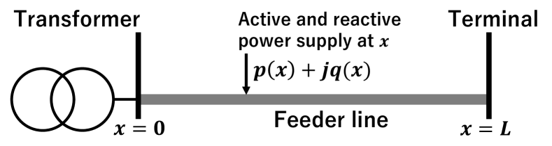
Throughout this paper, we consider a power distribution system where the feeder line is extended in a straight line from the transformer to the terminal as shown in Fig. 1. Note that electrical loads and electric power generations are typically connected at discrete locations on the feeder line. The electrical load is supposed to consume power from the feeder line, and the electric power generation, e.g. PV (photovoltaic) power generations are assumed to supply power to the line. For EVs, it is supposed not only to consume but also to supply power electricity. We assume that no electrical load is connected at the terminal of the feeder line.
Mathematically, the position variable on the feeder line is defined as . We suppose that [m] for the transformer (starting point) and [m], for the terminal of the feeder line, where is the length of the feeder line. Let and be the active and reactive powers at position over the feeder line, respectively. If holds, denotes the active power supply flowing to the feeder line at . On the other hand, holds, is the active power consumption flowing from the line at . The same physical meaning holds true for the reactive power . As we have assumed that no electrical load is connected at the terminal of the feeder line, the following boundary conditions also hold for active and reactive powers at the terminal:
| (1) |
Under the above setting on the feeder line, the spatial variation of the distribution voltage profile on the line is described by the nonlinear ODE model (See Chertkov et al. (2011), Tadano et al. (2022)), which is the following set of the ODEs (2)-(5):
| (2) | ||||
| (3) | ||||
| (4) | ||||
| (5) |
where , , , and represent the voltage phase, voltage amplitude, supplemental variable, and voltage gradient at position of the feeder line, respectively. In (4) and (5), is the conductance per unit length at position , which are assumed to be constant and positive, i.e. . Moreover, is the susceptance per unit length at position , which are assumed to be constant. Note that the susceptance can take both positive and negative values different from the conductance . The boundary condition for the set of ODEs (2)-(5) is given by the following equalities (See Chertkov et al. (2011), Tadano et al. (2022)) in per unit (p.u.) value:
| (6) |
In (6), the first and second equalities imply that we use the voltage amplitude and phase at the transformer as the reference values. From the assumption that no electrical load is connected at the terminal, the third and fourth equalities are imposed as the boundary condition.
By gathering the ODEs (2)-(5), we can be prove that the active power and reactive power satisfy the following ODEs in terms of the voltage amplitude and phase :
| (7) | ||||
| (8) |
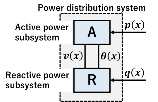
In this paper, the systems described by the ODEs (7) and (8) are called an active power subsystem and a reactive power system , respectively. From a system and control viewpoint, the voltage amplitude and phase can be regarded as the states (and become the outputs simultaneously) of each subsystem. Also, the active power and reactive power can be regarded as inputs to each subsystem. The block diagram of these subsystems is shown in Fig. 2. Note that there is no clear input-output relationship between the two subsystems via and . Therefore, we follow the framework of the behavioral system theory (See Willems (1991)) that enables us to treat such cases. For this reason, the tips of the arrows are removed in the diagram.
2.2 Dissipativity of active and reactive power subsystems
In terms of a complex-valued power, the ODEs (7) and (8) of the active and reactive power subsystems can be combined into a single ODE
| (9) |
From a viewpoint of dissipation theory, we can also regard the active power and reactive power as the supply rates at position for the subsystems and , respectively. The reason is that these power supplies electric powers to the considered power distribution system. Thus, we can investigate dissipativity for each subsystem.
To examine the dissipativity for the subsystems and , we define the function by
| (10) |
We can prove that this function coincides with the supplemental variable in the nonlinear ODE model (2)-(5) by a simple computation. The gradient of satisfies the equality
| (11) |
In addition to , we define the function by
| (12) |
By computing the gradient of this function, the function satisfies the equality
| (13) |
Substituting (11) and (13) into the first and second terms of the left-hand side of (9), respectively, we have the equality
By solving for the gradient of the linear combinations of the two functions in (10) and (12), we have
| (14) |
where is the quadratic function defined by
| (15) |
Note that it is clear that is a positive definite function from the above equation. The real part of (14) is described by the following equality:
| (16) |
From the imaginary part of (14), we can also derive the equality
| (17) |
Based on these equalities, we have the following theorem for the dissipativity of the active and reactive power subsystems in the sense of dissipation equality. The proof follows by applying Definition 1 to the equalities (16) and (17).
Theorem 1
Consider the active power subsystem in (7) and reactive power system in (8). Then, we have the following statements (i) and (ii).
-
(i)
The active power subsystem is dissipative with respect to the supply rate . Moreover, the functions and are the flux and dissipation rate, respectively, with respect to the supply rate .
-
(ii)
If holds, the reactive power subsystem is dissipative with respect to the supply rate . Moreover, the functions and are the flux and dissipation rate, respectively, with respect to the supply rate . If holds, is not dissipative with respect to the supply rate .
In Theorem 1, we have shown that the functions and correspond to the dissipation rates in the active and reactive power subsystems. In the next subsection, we verify that these dissipation rates are consistent with the well-known distribution loss in power systems.
2.3 Physical interpretation of dissipation rates
In this subsection, we discuss an interpretation of the function corresponding to the dissipation rates in both active and reactive subsystems.
We consider the phasor representation of the voltage at position , where the symbol “” over a complex variable stands for the phasor representation of the variable, not time derivative of the variable. The gradient of this phasor representation and its complex conjugate are computed by the following equations:
where the symbol “” denotes the complex conjugate. Then, we can prove that the product of the gradient and the complex conjugate coincides with as follows:
We also see that the gradient of the voltage can be described by the phasor representation of the current at position as follows:
where and are the resistance and reactance of the feeder line per unit length, respectively. Note that these constants satisfy the equality . By computing the second term corresponding to the dissipation rate on the right-hand side of (14), we have
| (18) |
where is the current amplitude of . The real part of the right-hand side of (18) satisfies the equality
Thus, we can verify that this real part is consistent with the well-known fact that the loss due to active power distribution is proportional to the square of the current (See Sugihara and Funaki (2019)). We can also prove that, if holds, the distribution loss of the reactive power can be represented by the square of the current as follows:
3 Dissipativity of voltage and phase subsystems
In this section, the entire distribution system considered in the previous section is transformed to the subsystems corresponding to the voltage amplitude and phase. As a main result, we show the dissipativity of these subsystems. Furthermore, as a physical interpretation of these results, we show that the typical phenomena related to the gradients of the voltage amplitude and phase are induced from the dissipativity of these subsystems. Finally, we provide a discussion on the reduction of the distribution loss in the entire system. See Appendix A for the dissipation theory for one-dimensional nonlinear systems with possibly noncausal independent variable.
3.1 Decomposition into subsystems
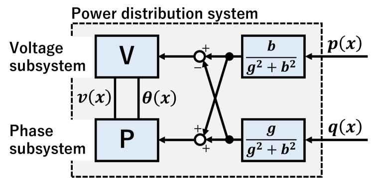
In this subsection, we consider the linear combinations of the active and reactive powers as new supply rates. Based on the combinations, the entire distribution system is decomposed into voltage subsystem and phase subsystem , which are defined in the next paragraph.
The ODEs (7) and (8) can be gathered by defining the appropriate vectors and constant matrices as follows:
| (19) |
Premultiplying (19) by the orthogonal matrix , we can derive the new equalities of the entire distribution system as
| (20) |
Considering the first column of the above equation, we obtain the following ODE:
| (21) |
The subsystem described by this ODE is called the voltage subsystem . Note that we can prove that the equalities (21) corresponds to the ODEs (4) which describes the derivative of the gradient of the voltage amplitude . For this reason, we mention as the voltage subsystem.
In addition to the ODE (21), we have another ODE
| (22) |
from the second column of (20). We can be verify that the equality (22) corresponds to the ODE (5) which describes the derivative of the supplemental variable . Since characterizes the derivative of the voltage phase , we call the subsystem the phase subsystem .
We provide the block diagram of the entire system consisting of the voltage and phase subsystems in Fig. 3.
3.2 Dissipativity of voltage and phase subsystems
In this subsection, we show the dissipativity of the voltage and phase subsystems defined in the previous subsection. The result of this subsection can be regarded as a main result of this paper.
From (13) and (15), we have the equality
By substituting this equality and (11) into (20), the equality (20) can be rewritten in terms of and as follows:
| . |
From the above equality, we have the following equalities on the gradient of and :
| (23) | ||||
| (24) |
Based on the above computation, we have the following theorem which shows the dissipativity of the subsystems and in the sense of dissipation equality. This theorem can be regarded as a main result of this paper. The proof follows from the equalities (23), (24) and Definition 1.
Theorem 2
Consider the voltage subsystem in (23) and phase subsystem in (24). Then, we have the following statements (i) and (ii).
-
(i)
The voltage subsystem is dissipative with respect to the supply rate . Moreover, the functions and are the storage function and dissipation rate, respectively, with respect to the supply rate .
-
(ii)
The phase subsystem is lossless with respect to the supply rate . Then, the functions is the flux with respect to the supply rate .
In the next subsection, a physical interpretation of Theorem 2 is clarified in detail from a viewpoint of electrical phenomena related to the gradients of the voltage amplitude and phase in typical power distribution systems.
3.3 Physical interpretation of main result
By computing the integrals of the supply rates in the dissipation equalities (23) and (24), and by substituting the boundary condition (6) into these integrals, we have the following equalities:
| (25) | ||||
| (26) |
The equalities (25) and (26) are important because they characterize the relationship between the active and reactive powers, the transmission losses, and the gradients of the voltage amplitude and phase at the transformer. In particular, these equalities correspond to the equalities obtained from the integral of the dissipation equalities of the voltage and phase subsystems, respectively. Each equality contains the gradients of the voltage amplitude and phase at the transformer. These facts are another reason that we call the subsystems described by the ODEs (23) and (24) the voltage and phase subsystems, respectively.
In the remainder of this subsection, we address a conventional power distribution system consisting of only loads, and a current power distribution system including PVs and EVs as typical power distribution systems supposed in this paper. By applying Theorem 2 to this system, we clarify a physical interpretation of the theorem.
3.3.1 3.3.1 Conventional power distribution system:
In the following, we consider a conventional power distribution system, and give a physical interpretation of the statement in Theorem 2. Such distribution system is known to have the following properties on the susceptance and the active and reactive powers:
-
•
The effect due to an inductance of the feeder line is dominant. This implies that the susceptance satisfies and .
-
•
PVs and EVs are not installed to the feeder line. In addition, loads are connected to spatially discrete positions. This implies that the active and reactive powers have nonpositive values, i.e. and hold at any position .
Since the active and reactive powers are nonpositive, the integral of the supply rate of is nonpositive in the left hand side of the (25):
For this reason, the dissipativity is not satisfied in the sense of nonnegativity of the integral of the supply rate over the infinite lengths of the integral domain, which are considered in Pillai and Willems (2002). This is also due to the fact that we consider the space as a finite interval. On the other hand, since there is a power consumption of the connected load, a current flows from the feeder line to the load. This implies that distribution loss occurs over the line. Thus, the integral on the right-hand side of (25) becomes nonnegative as follows:
In such a case, for the equality (25) to hold, we have the inequality
| (27) |
at the transformer (). This inequality indicates the occurrence of a voltage drop on the feeder line (Machowski et al. (2008)).
Moreover, considering (26) for the phase subsystem , the sign of the phase gradient at the transformer is indefinite depending on the values of the active and reactive powers from the equality
Combining the above equality with , we see that the active and reactive powers satisfy the inequality
if and only if the following inequality holds:
| (28) |
The above inequality corresponds to the delay of the voltage phase which typically occurs in conventional power systems (Machowski et al. (2008)).
The above series of the observation is consistent with typical phenomena observed in conventional power distribution systems, which shows a validity of our main result given in Theorem 2.
3.3.2 3.3.2 Power distribution system with PVs and EVs:
In a current power distribution system including PVs and EVs, the active and reactive powers at the position , where the PVs or EVs are connected, may have positive values. This implies that and hold for the position . In such a case, the following inequality typically holds in the first term on the left side of the (25):
This implies that the integral of the supply rate of the voltage subsystem possibly becomes nonnegative. Thus, contrary to the conventional power distribution systems, the dissipativity is guaranteed only by the integral of the supply rate. However, for some values of and , the net power supply will exceed the distribution loss in the right side of the (25). Then, it is necessary that the inequality
| (29) |
holds in the second term of the left-hand side of (25). The above inequality implies that a reverse power flow occurs on the feeder line.
In addition to the voltage subsystem, considering the equality (26) for the phase subsystem , the gradient of the voltage phase at the transformer can take both positive and negative values depending on the active and reactive powers from the following equality:
Combining the assumption with the above equality, we see that the active and reactive powers satisfy the inequality
if and only if the following inequality holds:
| (30) |
The above inequality shows an occurrence of a phase advance on the feeder line, which often occurs in current power distribution systems including PVs and EVs.
We can see that the above discussion is consistent with typical phenomena observed power distribution systems including PVs and EVs. Therefore, they also show a validity of the main result given in Theorem 2.
3.4 Discussion on reduction of distribution losses
In this subsection, we discuss a reduction of the dissipation loss based on the main result.
From (25), the integral of the dissipation rate can be expressed as
| (31) |
We have shown that the distribution loss is determined by the dissipation rate of the voltage subsystem in the previous subsection. The left-hand side of the above equality corresponds to the net distribution loss of the entire distribution system. Thus, the equality (31) shows that the net loss is characterized by the supply rate of the voltage subsystem and the voltage gradient at the transformer (). In more detail, to reduce the net distribution loss, it is important to attenuate the effect of the voltage gradients caused by transformers by an appropriate injection of both active power and reactive powers. Such a theoretical discussion for reducing overall distribution losses has not been considered so far in the framework of the nonlinear ODE model. Therefore, the discussion given here can be considered as one of the contributions of this paper. It is desired to derive appropriate design methods for both active and reactive power in our future work.
4 Conclusion
In this paper, we have shown dissipativity of the subsystems corresponding to the active and reactive powers of the power distribution system consisting of a straight feeder line. As a main result, we have proved the dissipativity of the voltage and phase subsystems. We have also provided a physical interpretation of the main results based on the dissipation equalities of these subsystems. Finally, we have given a discussion for a reduction of distribution losses based on the dissipation rate of the voltage subsystem.
One of the future work is the voltage control of the actual distribution system, which also takes into account the distribution losses due to active and reactive power injections. In addition, it is desired to generalize the results of this paper to the case where the bifurcations are contained in the feeder line.
Appendix A Dissipation Theory for Spatial One-Dimensional Systems
In this appendix, we provide a preliminary notion of the dissipation theory (Willems (1971), Willems (1972a), Willems (1972b)) to consider dissipativity of distribution systems described by the nonlinear ODE models in this paper.Specifically, we integrate the dissipation theory (See Pillai and Willems (2002)) for linear -dimensional systems with both time and space as independent variables, and nonlinear one-dimensional systems with time as an independent variable (See Khalil (2002)).Based on this integration, we extend the framework to nonlinear one-dimensional systems with independent variables, e.g. space, that are not necessarily causal such as time, and are contained in a finite interval.
Consider a nonlinear system with the independent variable , where is the finite interval to which belongs. We suppose that is an independent variable, e.g. space, which is not necessarily causal such as time. Then, is described by the following nonlinear ODE:
| (32) |
where and are the state and input of this system. In (32), is a nonlinear function.
We give the definition of the nonlinear systems considered in this paper as follows.
Definition 1
Consider a nonlinear system in (32) with the independent variable , where is the finite interval to which belongs. Let be the power delivered to the nonlinear system in (32). We call supply rate of the system .
-
(i)
The system is called dissipative with respect to the supply rate if there exist functions and satisfying the inequality
(33) and for any .
-
(ii)
The system is called dissipative with respect to the supply rate if there exists a function satisfying the inequality
(34) for any .
In (33) and (34), the functions and are called flux and dissipation rate for with respect to the supply rate . Moreover, the equalities (33) and (34) are called the dissipation equality.
We can regard as the power delivered to the system . Moreover, the flux corresponds to the energy which moves over the interval . From this point, the dissipation equality (33) implies that the spatial variation of the energy of the system does not exceed the power supplied to the system due to the existence of the dissipation rate which is a nonnegative function. This implies that the system dissipates energy to the external environment of the system. Note that we do not introduce time as an independent variable in this paper. For this reason, any storage function do not appear in this paper, which expresses the internal energy in the ordinary dissipation theory (Pillai and Willems (2002), Willems (1971) and etc.).
By computing the integral of the dissipation equality (20) from to , we have the inequality
If we consider the space as the interval of infinite length, it is known that the dissipativity of the system is guaranteed only by the integral of the supply rate, i.e. the net power supplied to the system (See Pillai and Willems (2002)). However, the space is restricted to an interval of finite length in this paper. Therefore, the compensation by the spatial variation of the flux results in dissipation of the energy of the entire system.
References
- Arcak (2007) Arcak, M. (2007). Passivity as a Design Tool for Group Coordination. IEEE Transactions on Automatic Control, 52(8), 1380–1390.
- Chertkov et al. (2011) Chertkov, M., Backhaus, S., Turtisyn, K., Chernyak, V., and Lebedev, V. (2011). Voltage Collapse and ODE Approach to Power Flows: Analysis of a Feeder Line with Static Disorder in Consumption/Production.
- Gan et al. (2015) Gan, L., Li, N., Topcu, U., and Low, S. (2015). Exact Convex Relaxation of Optimal Power Flow in Radial Networks. IEEE Transactions on Automatic Control, 60(1), 72–87.
- Khalil (2002) Khalil, H. (2002). Nonlinear Systems. Prentice Hall, Third edition.
- Machowski et al. (2008) Machowski, J., Bialek, J., and Bumby, J. (2008). Power System Dynamics: Stability and Control. Jon Wiley & Sons, Ltd, Second edition.
- Pillai and Willems (2002) Pillai, H. and Willems, J. (2002). Lossless and Dissipative and Distributed Systems. SIAM Journal on Control and Optimization, 40(5), 1406–1430.
- Qu and Simaan (2014) Qu, Z. and Simaan, M. (2014). Modularized Design for Cooperative Control and Plug-and-Play Operation of Networked Heterogeneous Systems. Automatica, 50(9), 2405–2414.
- Sugihara and Funaki (2019) Sugihara, H. and Funaki, T. (2019). Analysis on temperature dependency of effective ac conductor resistance of underground cables for dynamic line ratings in smart grids. In 2019 IEEE 21st International Conference on High Performance Computing and Communications; IEEE 17th International Conference on Smart City; IEEE 5th International Conference on Data Science and Systems (HPCC/SmartCity/DSS), 2637–2643.
- Tadano et al. (2022) Tadano, H., Susuki, Y., and Ishigame, A. (2022). Asymptotic assessment of distribution voltage profile using a nonlinear ode model. Nonlinear Theory and Its Applications, IEICE, 13(1), 149–168.
- Willems (1971) Willems, J. (1971). Least Squares Stationary Optimal Control and the Algebraic Riccati Equation. IEEE Transactions on Automatic Control, AC-16(6), 621–634.
- Willems (1972a) Willems, J. (1972a). Dissipative Dynamical Systems-Part I: General Theory. Archive for Rational Mechanics and Analysis, 45, 321–351.
- Willems (1972b) Willems, J. (1972b). Dissipative Dynamical Systems-Part II: Linear Systems with Quadratic Supply Rates. Archive for Rational Mechanics and Analysis, 45, 351–393.
- Willems (1991) Willems, J. (1991). Paradigms and Puzzles in the Theory of Dynamical Systems. IEEE Transactions on Automatic Control, AC-36(11), 259–294.