Are Code Pre-trained Models Powerful to Learn
Code Syntax and Semantics?

Abstract.

A large amount of code pre-trained models have contributed significant development to code intelligence. Analysis of these pre-trained models also has revealed that they can effectively learn program syntax. However, these works are limited in analyzing code syntax and their distance-based approaches are not accurate due to the curse of high dimensionality. Furthermore, the study of the learnt program semantics of these models is rarely discussed. To further understand the code features learnt by these models, in this paper, we target two well-known representative code pre-trained models (i.e., CodeBERT and GraphCodeBERT) and devise a set of probing tasks for the syntax and semantics analysis. Specifically, on one hand, we design two probing tasks (i.e., syntax pair node prediction and token tagging prediction) to manipulate AST for the understanding of learnt program syntax. On the other hand, we design two tasks (i.e., semantic relationship prediction and semantic propagation prediction(inGraph) ) on the constructed control flow graph (CFG), data dependency graph (DDG) and control dependency graph (CDG) for the learnt program semantic analysis. In addition, to understand which kind of program semantics these pre-trained models can comprehend well, we conduct the statistical analysis for attention weights learnt by different heads and layers.

Through extensive analysis in terms of program syntax and semantics, we have the following findings: 1) Both CodeBERT and GraphCodeBERT can learn the program syntax well. 2) Both CodeBERT and GraphCodeBERT can learn program semantics to different extents. GraphCodeBERT is superior to CodeBERT in learning program control flow and data dependency information but has a similar capability to CodeBERT in learning control dependency information. 3) Both CodeBERT and GraphCodeBERT can capture program semantics in the final layer of representation, but different attention heads and layers exhibit different roles in learning program semantics.

1. Introduction

Recently, code pre-trained models have attracted widespread attention from academia and industry due to their superior performance on many code-related tasks such as vulnerability detection (Zhou et al., 2019), program repair (Drain et al., 2021; Li et al., 2022) and source code summarization (Liu et al., 2020). Compared with traditional feature engineering, which relies on hand-crafted features designed by human experts for feature extraction, these learning-based approaches are able to learn effective features automatically from the data, hence greatly reducing the time costs and labor costs. Furthermore, compared with the supervised models for code such as graph neural networks (Allamanis et al., 2017; Li et al., 2015), the unsupervised code pre-trained models rely on self-attention (Vaswani et al., 2017) to learn contextual code representations from a massive amount of unlabeled data. Due to the utilized scale of datasets and the advanced learning strategies, these pre-trained models are usually superior to supervised techniques and have more powerful generalization ability across different code-related tasks. Hence, the pre-training techniques have become a new paradigm in AI for SE (AI4SE) and attracted broad research from different aspects to make contributions to the development of code intelligence.

A great number of works (Kanade et al., 2019; Feng et al., 2020; Guo et al., 2020; Lu et al., 2021; Svyatkovskiy et al., 2020; Buratti et al., 2020; Karampatsis and Sutton, 2020; Wang et al., 2021; Ahmad et al., 2021; Liu et al., 2023) explore the way to improve the performance of code pre-trained models over downstream tasks. Although these works have confirmed the improvements in different downstream tasks, one core question still exists. That is “What kind of knowledge can these pre-trained models learn?” Specifically, this question can be further divided into two sub-questions (i.e., “Can code pre-trained models capture program syntax well?” and “What kind of program semantics can code pre-trained models learn?” Intuitively, if a pre-trained model such as CodeBERT (Feng et al., 2020) or GraphCodeBERT (Guo et al., 2020) utilizes masked language modelling (i.e., MLM, a pre-training task to randomly mask some tokens in a sequence and requires the model to recover these masked tokens) as one of the pre-training tasks to learn the contextual representations, the model is able to learn code syntax and semantics. One example is presented in Figure 1. When MLM masks the syntax keywords “if” and “return”, the model has to understand the code syntax for the correct prediction. Similarly, for the semantic keywords such as “int” and “float”, if MLM masks both, the model has to consider the whole context of the program to infer the masked variable type. Previous works have been done to study the aforementioned questions to some extent, especially for the first sub-question, but more work is needed to fully answer what kind of knowledge these code models learn. Wan et al. (2022) use the distances from AST to train a probing classifier and also analyze the attention weights for code syntax. López et al. (2022) projects the AST and code vector representation into a syntax subspace for analysis. Although both works have confirmed that code pre-trained models can capture program syntax well, they will potentially suffer from the curse of high dimensionality and lead to an inaccuracy result (more details in Section §2). At the same time, the second question, according to the best of our knowledge, has not been answered so far.

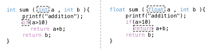
Figure 1. MLM can learn syntax and semantics via masking syntax or semantic tokens.

To address the aforementioned challenges, in this paper, we propose our approach to answer both questions. We choose CodeBERT (Feng et al., 2020) and GraphCodeBET (Guo et al., 2020) for the analysis since both are representative and our analysis is also orthogonal to other code pre-trained models. Specifically, we design a set of probing tasks in terms of code syntax and semantics for deep analysis. Two syntax probing tasks (i.e., syntax node pair prediction and token syntax tagging prediction) are proposed, which manipulate AST to help us understand the ability of the pre-trained model in learning code syntax. Syntax node pair prediction aims to analyze if the vector representations of two syntax-close token spans are syntax close while token syntax tagging prediction aims to if the vector representation contains the grammar rule. Furthermore, we propose three semantic probing tasks (i.e., semantic relation prediction, semantic propagation prediction and type inference) to analyse what kind of code semantics CodeBERT and GraphCodeBERT can learn well. Semantic relation prediction aims to detect whether the vector representations of two semantic-related token spans are semantically related, while semantic propagation prediction aims to analyze if one token span can potentially affect the program output. The type inference aims to infer the variable type. We compare the consistency of the layer roles between CodeBERT and GraphCodeBERT through Spearman’s $\rho$ in terms of syntax and semantics on all proposed probing tasks. We further conduct the statistical analysis for the attention weights learned by different heads and layers across CodeBERT and GraphCodeBERT to comprehensively understand the role of each layer in learning code semantics. Through extensive analysis, we have the following findings: 1) CodeBERT and GraphCodeBERT can learn program syntax well by analysing syntax probing tasks. 2) Both CodeBERT and GraphCodeBERT can learn code semantics to some extent. Specifically, GraphCodeBERT is superior to CodeBERT in learning control flow and data dependency information while has a similar performance on learning control dependency information through the analysis of semantic probing tasks. 3) Different heads and layers play different roles in learning program semantics through the statistical analysis of attention weights. In summary, our contributions are summarized as follows:

• We propose a group of probing tasks to analyze the properties of pre-trained code models in terms of syntax and semantics.

• We find that the pre-training task of masked language modelling (MLM) ensures the pre-trained code models learn code syntax and semantics; however, learning code syntax is better than learning code semantics using MLM.

• We find that attention heads play different roles in representing code semantics. GraphCodeBERT is superior to CodeBERT in learning control flow and data dependency, but both are weak in learning control dependency. We hope this finding can inspire the follow-up researchers to incorporate program control dependencies in the pre-trained models for enhancement.

2. Motivation

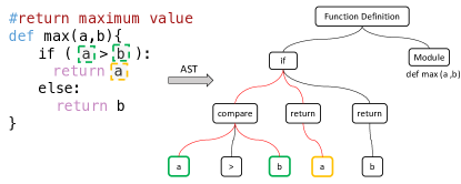
Figure 2. A simple code snippet with its AST.

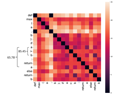
Figure 3. Euclidean distance of token representations.

In this section, we discuss the limitation of existing works regarding the analysis of code pre-trained models. The most related public works to our study are Wan et al. (2022) and López et al. (2022). Specifically, Wan et al. (2022) proposed to design the probing analysis based on the node distance  in AST to explore whether these code pre-trained models can learn code syntax. Furthermore, the analysis is under the assumption that if two nodes in the code have close syntax, they may have a small distance in AST, and similarly, the vector representation distance, such as the euclidean distance of two nodes encoded by the code model, is small (i.e., close syntax $\rightarrow$ small node distance, close syntax $\rightarrow$ small representation distance). Similarly, López et al. (2022) proposed to project the vector representation space of code models into a learned syntactic subspace that is assumed to encode the distances in AST. Hence, both works map the node distance in AST to the vector representation distance encoded by pre-trained code models and assume that they are positively related.

However, code vector representation space is a high-dimension space. For example, CodeBERT forms a 768-dimensional space but node distance in AST is a low dimension space. Therefore, the traditional distance metrics will not work well due to the curse of high dimensionality (Mirkes et al., 2020; Aggarwal et al., 2001). The mapping from high-dimension space to low-dimension space may not be accurate; the small distance in the AST may not definitely represent the small euclidean distance in the high-dimension space, i.e., their correlation is weak theoretically. Here, we give a simple example for better illustration. As shown in Figure 2, given a function with its parsed AST. We can see that the node distance between the variable “a” and “b” from the if-condition (marked with green squares) is 2 and the node distance between this variable “a” (green square) and the variable “a” (orange square) from the return statement is 4. Hence, we can get the conclusion that in the low-dimension space, the variable “a” from the if-condition is close to the variable “b” and they are syntax-closer than the variable “a” from the return statement. In Figure 3, we present the euclidean distance for the above variables. In particular, we encode this function by CodeBERT and calculate the euclidean distance between the token vector representations for these variables. We can see that the euclidean distance for the variable “a” (green square) and the variable “b” (green square) from the if-condition is 85.45 while the variable “a” (green square) from the if-condition and the variable “a” (orange square) from the return statement is 65.78. The smaller distance indicates that the variable “a” from the if-condition and the variable “a” from the return statement are closer than the variable “b” from the if-condition in high-dimension space. Hence, we can get the conclusion that the distances in the low space and high space are not consistent and they may not be positively related. To avoid the transformation between the high space and low space, we need to explore new approaches for code syntax analysis.

In addition, both works only explore the capability of code pre-trained models in learning code syntax while the analysis in learning code semantics is less touched. It is vital to understand the capability of these code pre-trained models in learning code semantics and exploring which kind of code semantics can these models learn well is meaningful.

3. Analysis Methodology

In this section, we introduce our analysis of the probing approaches for code syntax and semantics. We future compare the consistency of the layer roles between CodeBERT and GraphCodeBERT through Spearman’s $\rho$ on all tasks.

3.1. Syntax Probing

To avoid the inaccuracy caused by the transformation from high space to low space, in this section, we propose two kinds of syntax probing tasks, which directly predict the attributes of nodes in AST for analysis.

3.1.1. Syntax Node Pair Prediction

Given a source code, we can obtain the AST for this code and we further split the whole AST into different subtrees. Each subtree is one statement from the original code and we name it as one basic syntax unit. Because each syntax unit represents one statement from the code, we can conclude that the nodes in a unit are syntax-close. Hence, this task is designed to predict any pair of nodes in AST belonging to a subtree. In particular, we present an example for better illustration. As shown in Figure 4, there is a function “f” whose corresponding AST is presented on the right hand. For this AST, we split it into different units marked with different colours. For example, the node of “=” in the red unit, should be syntax close to its left nodes in this unit such as the node of “int” and “a”. Hence, they are labelled with “1” for the positive samples. For the node of “int” and “a” in another unit (marked with green), since they belong to another unit, hence they are labelled with “0” as the negative samples. Formally, this task can be formulated as follows:

$$classifier(n_{0},n_{1})=\begin{cases}1&n_{0}\in T_{i}\cap n_{1}\in T_{i}\\ 0&n_{0}\in T_{i}\cap n_{1}\in T_{j}\end{cases}$$

where, $i\neq j$, $T_{i}$ and $T_{j}$ are two different units (i.e., subtrees) in AST and $n_{0}$ and $n_{1}$ are the nodes in the unit. We train a binary probing classifier to learn whether any pair of nodes belong to a subtree of AST for analysis.

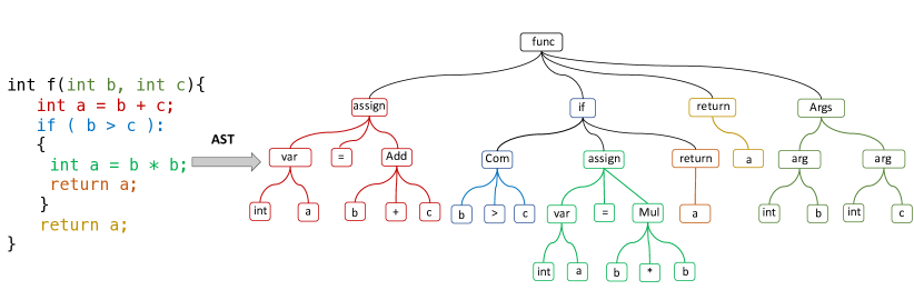
Figure 4. Syntax Pair Node Prediction.

3.1.2. Token Syntax Tagging

We further design another syntax probing task that is different from the previous one. Since the task of syntax pair node prediction is a binary classification task, which is easier for the probing model to make the correct predictions. To increase the difficulty of the prediction, we propose a multiple-classification task, namely token syntax tagging. Since a programming language can be described as a set of grammar rules. For example, there are five simple rules for a programming language as follows:

$$\begin{cases}op1::=+\>|\>-\\ op2::=*\>|\>/\\ expression::=Term\{\>op1\>Term|\>op1\>Term\}\\ Term::=Factor\{\>op2\>Factor|\>op2\>Factor\}\\ Factor::=Number\>|\>(expression)\end{cases}$$

It denotes that a programming language allows addition, subtraction, multiplication and division of numbers. Hence, we can assign a grammar label for each token in the code. For example, the symbol “+” has a type of “op1”. Furthermore, since some grammar labels are highly abstracted, for example, the variable name is labelled with “identifier” by the grammar rule, but it has different semantics in the context. If it is in the function declaration, it is actually an argument for this function; similarly, if it is in the class invocation, it is a class attribute. Hence we design concrete labels for these abstracted tokens. Specifically, we design 36 tagging labels for Java and 33 labels for C/C++. We further present an example with the corresponding syntax label in Figure 5. The detailed information of these used labels in this example is shown in Table 1. In particular, we can find that the tokens “(” and “)” have different syntax labels in different contexts. The parenthesis “( )” are labelled with “PE” in the if condition while the parenthesis “( )” are labelled with “AL” in the method invocation. We design the token syntax tagging to explore whether these models can learn the code syntax property from the programming grammar.

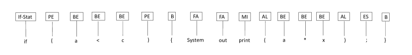
Figure 5. Token tagging.

Table 1. The tagging labels for the tokens used in Figure 5.

Label	Description
PE	Parenthesized expression
BE	Binary expression
B	Block
FA	Field access
MI	Method invocation
AL	Argument list
ES	Expression statement

3.2. Semantic Probing

The previous works mainly design a set of probing tasks to analyse the capacity of pre-trained code models in learning code syntax. However, the analysis of code semantics is less touched. In this section, we further propose three kinds of probing tasks to analyse the learnt code semantics for the supplement.

3.2.1. Semantic Relation Prediction

Similar to the task of syntax node pair prediction in Section 3.1.1, we also extract the control dependency graph (CDG), data dependency graph (DDG) and control flow graph (CFG) to predict whether the code pre-trained models can learn code semantics. Note that different from AST, in which each node only contains one token, each node in the constructed CDG, DDG and CFG has one original statement from the original code. We unify these tasks into a unified task namely semantic relation prediction. Formally, this task can be formulated as follows:

$$classifier(s_{0},s_{1})=\begin{cases}1&\exists g\in G,\quad s_{0}\in N_{i}\cap s_{1}\in N_{j}\cap\{N_{i}\xrightarrow{g}N_{j}\}\\ 0&\forall g\in G,\quad s_{0}\in N_{i}\cap s_{1}\in N_{j}\cap\{N_{i}\centernot{\xrightarrow{g}}N_{j}\}\end{cases}$$

where $N_{i}$, $N_{j}$ is the $i$-th node and $j$-th node in the constructed graph $G=\{CDG,DDG,CFG\}$ and each node contains one statement from the original code. $s_{0}$, $s_{1}$ denote the token span of the code in nodes $N_{i}$ and $N_{j}$ after tokenization. $\xrightarrow{g}$ means that there is an edge between tow nodes in $g$.

Figure 6(a), Figure 6(b) and Figure 6(d) demonstrates examples for the three semantic relationships. Figure 6(a) shows one control dependence example. The node $N_{4}$ is control dependent on the node $N_{3}$. Based on this fact, we label that the token span from $N_{3}$ is control dependent on the token span in $N_{4}$. Figure 6(b) illustrates one data dependence example. The node $N_{4}$ is data dependent on the node $N_{1}$. Figure 6(d) shows one example of a control flow graph. We have some execution order facts like that the node $N_{2}$ is executed after $N_{1}$ immediately. The token span of $N_{2}$ has a control-flow relationship with the token span of $N_{1}$.

3.2.2. Semantic Propagation Prediction

Dependence graphs of the program can represent code semantics (Horwitz and Reps, 1992). Data flow information is propagated in the dependence graph. It is a fact that any modification in the dependence graph potentially affects the program output. The implicit dependence flow propagation is one import program semantics. The semantic propagation task (alias inGraph) is defined by that

$$classifier(s_{0},s_{1})=\begin{cases}1&\quad s_{0}\in N_{i},s_{1}\in N_{j},N_{i}\in g\cap N_{j}\in g\\ 0&\quad s_{0}\in N_{i},s_{1}\in N_{j},N_{i}\in g\cap N_{j}\notin g\end{cases}$$

, where $g\in\{CDG,DDG\}$ , $s_{0}$ and $s_{1}$ are the token spans in the nodes of $g$. Figure 6(c) shows one example. The shadow box highlights the statements with the control dependence relationship. We expect the probing classifier can recognize that the “printf” statement is not in the dependence control graph.

3.2.3. Type Inference

The third semantic task is type inference, i.e., inferring the variable type in the code from its contextual representation. For example, we can mask the variable $a$ type in Figure 6(e), and then use the contextual representation of $a$ to infer its type. It is not possible to infer one variable type without context. For example, the type of “a” depends on the types of “b” and “c” in the statement “MASK a=b+c”. If “b” and “c” are int type, “a” should also be int. However, if “b” is int and “c” is float, “a” should be float.

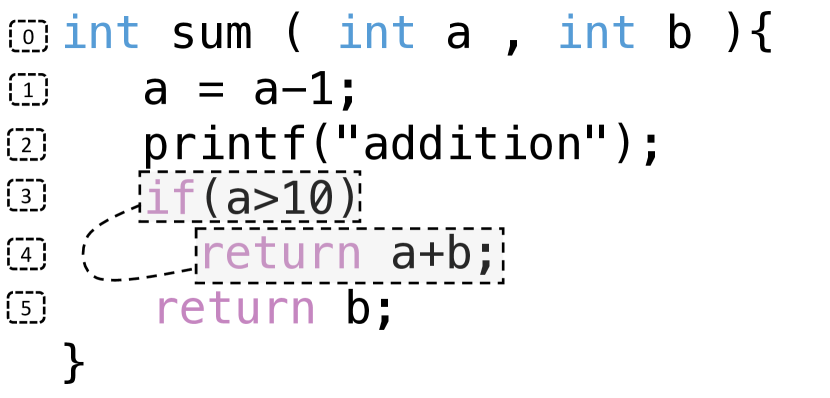
(a) control dependence.

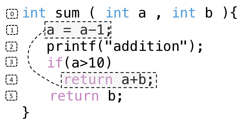
(b) data dependence.

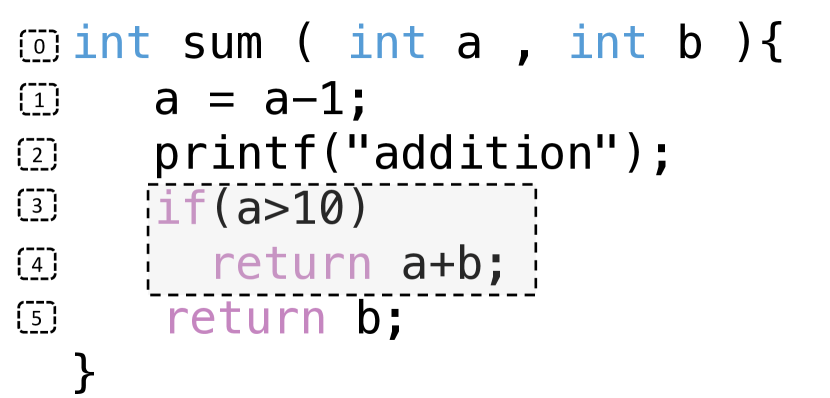
(c) inGraph.

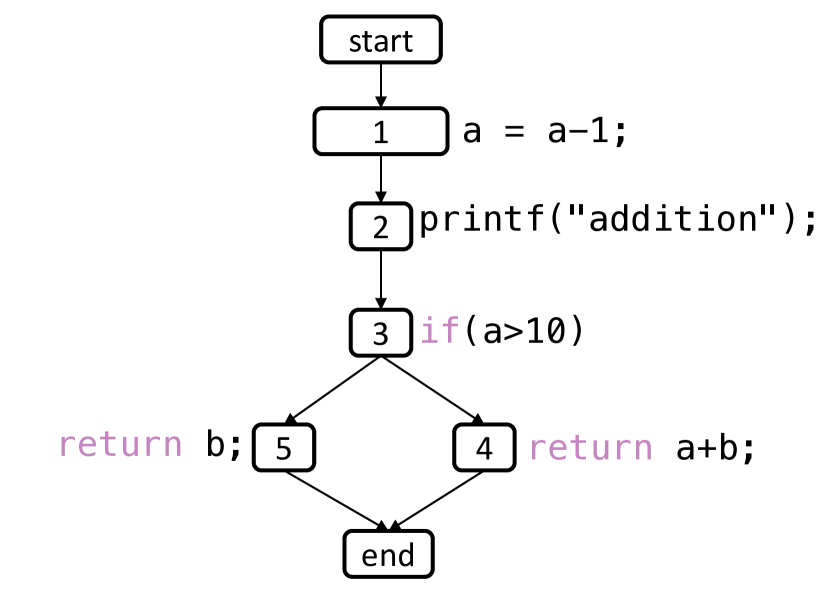
(d) control flow.

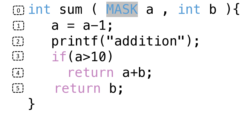
(e) type inference.

Figure 6. Examples about semantic probing.

3.3. Attention Analysis

We analyze the attention weights based on the program semantic relationships $G=\{CFG,DDG,CDG\}$ from §3.2.1 for every self-attention head at each layer. Given one node token span $s_{i}$ and a semantic-relationship type $g\in G$, we group the remaining input tokens into two sets $R_{1}$ and $R_{0}$, where $R_{1}$ consists of all tokens that have the semantic-relationship type to $s_{i}$, and the left tokens constitutes the set $R_{0}$. Then, based on $R_{1}$ and $R_{0}$, we group the attention weights related to $s_{i}$ into two sets, denoted $W_{1}$ and $W_{0}$. We apply the paired t-test  with the large sample size for each semantic type, i.e., control flow, data dependence, control dependence; null hypothesis $H_{0}:\mu_{d}=0$, and alternative hypothesis $H_{1}:\mu_{d}>0$, where $\mu_{d}$ is the true mean difference between $W_{1}$ and $W_{0}$ . Both CodeBERT and GraphCodeBERT contain twelve (12) encoder layers, and each encode layer has twelve (12) attention heads. We conduct the paired t-test in two different levels, layer-level analysis, and head-level analysis. On one hand, the layer-level test regards the attention heads from the same layer as one integration, and it helps to understand the role of each self-attention layer. On the other hand, head-level analysis investigates each attention head in each layer, providing us with more fine-grained views about self-attention. We also use the heatmap to visualize the attention weight distribution for $R_{1}$ and $R_{0}$. This can help us understand the role of each attention head in learning code semantics. We analyze more than 10K semantic inputs.

3.4. Probing Model

Probing Model We adopt the edge probing classifier (Tenney et al., 2019), as shown in Figure 7. Following the probing literature, parameters in the contextual representation encoder are fixed. We first get the contextual representation for each token from code models. Then, we fetch our targeted token spans that are related to the graph or tree node. Next, we use one attention pool to map the span vectors into one fixed-size vector before we forward them to the probing classifier (a MLP classifier).

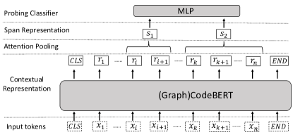
Figure 7. Probing model.

Table 2. Probing tasks.

Probing Task	Target	Description	Related RQ
Syntax Pair Node Prediction	syntax	predicting the syntax close nodes	RQ1
Token Tagging		infer Token grammar/syntax label
Semantic Relation	semantics	predicting semantic relationships among tokens	RQ2
Semantic Propagation (inGraph)		judge if the information of one token span can affect the program output
Type Inference		infer the types of variables in the context
Weight Analysis	semantics	analyze the attention weights based on the program graphs	RQ3

3.5. Research Questions

We have three (3) research questions, as shown in the below list. First, we validate if the representations from code models have encoded the syntax relationship among code tokens from AST and the programming language rules. Then, we check the extent to which code models learn semantic code properties. Finally, we give insights into the relationship between attention weights and code semantic properties.

• RQ1. Do code models learn the programming language syntax from the view of syntax facts from AST and the programming language grammar rules?

• RQ2. Can code models encode the code semantic relationship existed in the program analysis graphs (control flow, control dependence, and data dependence)?

• RQ3. What role do the attention heads play in the code semantics?

4. Evaluation Setup

In this section, we mainly introduce the evaluation setup of this work.

4.1. Dataset and Pre-processing

We use two datasets, Java250 (Puri et al., 2021) and POJ-104 (Mou et al., 2016), which are summarized in Table 3. To probe code models, we also have to extract syntax data and semantic data as shown by Figure 8. We refactor the code in a google-java-format tool and a clang-refactor tool because the refactored code is friendly and used for token alignment between the graphs and the model input. We use the static analysis framework Joern  and AST parser  to extract program graphs and AST. For program graphs, we also merge the redundant nodes if the code of one node is a subset of its neighbour. Then, we extract the syntax relationship and semantic relationship among the code tokens as the probing datasets.

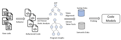
Figure 8. The workflow of data pre-processing.

Table 3. The statistics of the datasets.

Name	Train/Val/Test	Language	Task
Java250	75k/-/-	Java	Code Classification
POJ-104	32k/8k/12k	C/C++	Code Clone Detection

4.2. Experiment Control

4.2.1. Experiment Models

We experiment with two (2) pre-trained models, CodeBERT (Feng et al., 2020) and GraphCodeBERT (Guo et al., 2020). For three research questions, we refer to the random initialized CodeBERT and GraphCodeBERT as the baselines, denoted as CodeBERT_rand and GraphCodeBERT_rand. Compared with the baselines, we can see how code models benefit from pre-training in terms of syntax and semantics. The goals of the research questions are to study the extent to which BERT-based code models learns code syntax and semantics across different Transformer layers via self-attention and MLM.

4.2.2. Experiment Design

Probing analysis aims to illustrate whether or not a model has learned specific properties of code. Following the common practice (Liu et al., 2019; Rogers et al., 2020), we use a simple classifier MLP (multilayer perceptron). We study the extent to which CodeBERT and GraphCodeBERT encode syntax and semantics. We also want to investigate if pre-training can help CodeBERT and GraphCodeBERT understand code syntax and semantics. Therefore, we compare the pre-trained models with their randomly-initialized versions (denoted as CodeBERT_rand and GraphCodeBERT_rand). It is well known that the performance of the classifiers is affected by many factors, e.g., inputs, random seed, learning rate, optimizer, and batch size. To alleviate this issue, we repeat all experiments multiple times; for each repetition, we only change the random seeds. We use the same settings of learning rate, optimizer and batch size from the original papers. CodeBERT and GraphCodeBERT have 12 Transformer layers (denoted as $\mathbf{Layer_{1}}$-$\mathbf{Layer_{12}}$) plus one (1) embedding layer (denoted as $\mathbf{Layer_{0}}$). We apply our probing tasks for each Transformer layer and the embedding layer. This helps us understand the role of each layer.

4.3. Evaluation Metrics

We use three performance metrics, F1-score, Matthew’s correlation coefficient (MCC), and Accuracy. F1-score is the harmonic mean of precision and recall. F1-score is one standard method to measure model performance in information retrieval and machine learning, especially in natural language processing. However, F1-score does not take care of true negatives, and it can be misleading for imbalanced datasets. MCC is one reliable alternative to F1-score, and it considers the whole confusion matrix. Accuracy is the ratio of correct ones among the total number of predictions and measures how close the predictions are to true values. Multiple metrics enable us to measure the model from different angles. We also compute the performance difference between the pre-trained model (PLM) and its initialization version (PLM_rand), i.e., $diff=performance(PLM)-performance(PLM_{rand})$. The differences can reflect how many benefits we can gain from the pre-training.

5. Experimental Results

In this section, we present the experimental results to answer the designed RQ1-RQ3, and all experiments are repeated by multiple times and we use the mean values. As the global notation, we denote CodeBERT and GraphCodeBERT as CB and GCB, respectively. In our curve figures, the solid lines are for CodeBERT and the dash lines are for GraphCodeBERT.

5.1. Syntax Analysis (RQ1)

5.1.1. Syntax Pair Node prediction

Figure 9(a) and Figure 9(b) shows the results of the probing classifiers for syntax pair node prediction on Java250 and POJ-104 based on the representations from code models. X-axis is the layer index and Y-axis is the performance. $Layer_{0}$ is the embedding layer. $Layer_{1}$-$Layer_{12}$ are the Transformer layers. For this task, GraphCodeBERT (GCB) is a little better than CodeBERT (CB) in Figure 9(a) for Java250 when we check Accuracy(blue lines), F1(green lines) and MCC (yellow lines). However, the advantage is negligible in terms of ACC (blue lines) and F1 (green lines). This advantage disappears in Figure 9(b) on POJ-104; GraphCodeBERT and CodeBERT perform almost similarly. One interesting is that $Layer_{2}$ gets the best performance in Figure 9(a) and Figure 9(b). Then, the probing model performance decreases until $Layer_{7}$ and increases again. However, the increase stops at $Layer_{11}$ and the model performances sharply drops at $Layer_{12}$ in Figure 9(a) and Figure 9(b).

Figure 9(c) and Figure 9(d) illustrate the performance difference between the representations of code models (CodeBERT and GraphCodeBERT) and their random initialization (CodeBERT_rand and GraphCodeBERT_rand), respectively. We can see that $Layer_{0}$ (the embedding layer) gains a few benefits to encoding code syntax from pre-training, increasing by about 3% to 6%. With increasing the layer depth, the interest from pre-training slowly grows but decreases from $Layer_{11}$ to $Layer_{12}$. CodeBERT and GraphCodeBERT obtain almost the same benefits from pre-training in terms of code syntax.

5.1.2. Token Tagging

Figure 10(a) and Figure 10(b) demonstrate the results of the probing classifiers for Token Tagging on Java250 and POJ-104, respectively. We find that CodeBERT and GraphCodeBERT have no difference in understanding the programming language grammar in terms of ACC and MCC. However, CodeBERT is slightly better than GraphCodeBERT in terms of F1. At $Layer_{5}$, $Layer_{9}$, and $Layer_{10}$, the probing classifiers almost achieve the best performance. Similar to syntax pair node prediction, from $Layer_{11}$ to $Layer_{12}$, the model performances drop a lot.

Figure 10(c) and Figure 10(d) describe the performance difference between the representations from pre-trained models and the randomly initialized models on Java250 and POJ-104, respectively. Compared with the performance difference Figure 9(c) and Figure 9(d) for syntax pair node prediction, we find that $Layer_{0}$ for Token Tagging gets a little worse after pre-training, decreased by about 5% and 10%. It is reasonable because the two probing tasks prefer different syntax properties. Syntax pair node prediction task can be partially solved by identifying the token position, which results in $Layer_{0}$ shows benefits from pre-training for syntax pair node prediction due to its position embedding. In contrast, accurately tagging the tokens requires whole context information. We also find that the gains obtained from pre-training increase along with the layer depth. However, there still is a performance drop from $Layer_{11}$ and $Layer_{12}$.

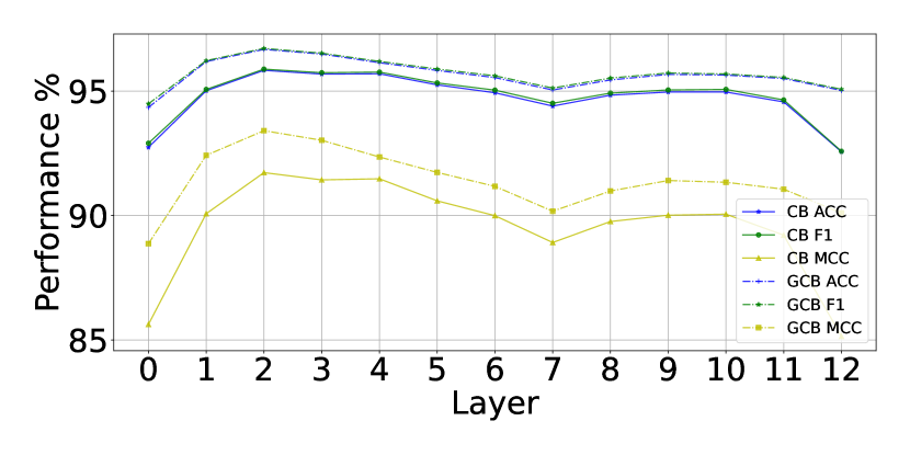
(a) Java250-AST.

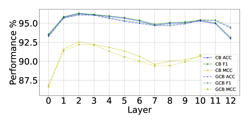
(b) POJ-104-AST.

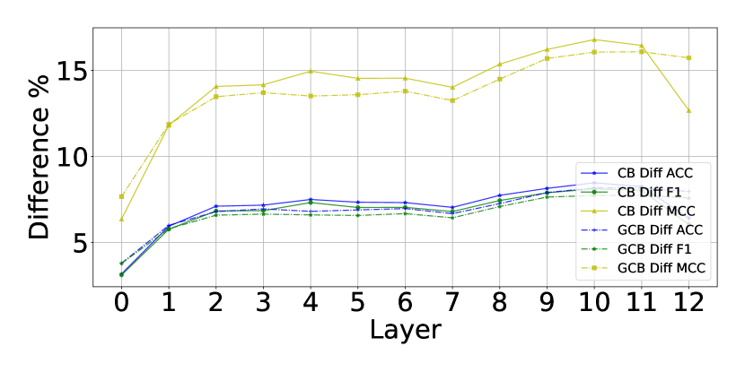
(c) Java250-AST-Diff.

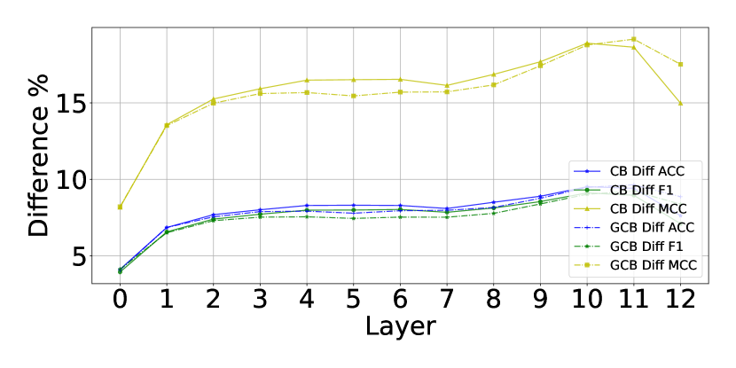
(d) POJ-104-AST-Diff.

Figure 9. Performance and Performance-Diff about Java250 and POJ-104 for Syntax Pair Node prediction (AST).

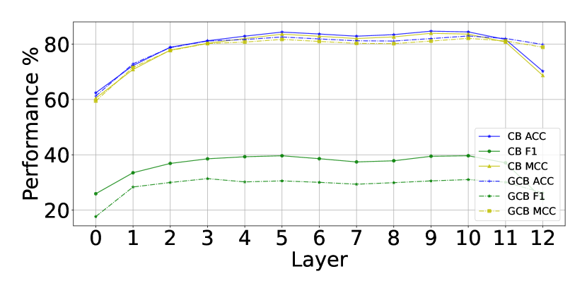
(a) Java250-Tagging.

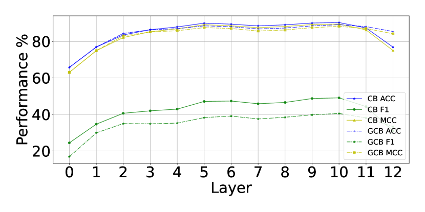
(b) POJ-104-Tagging.

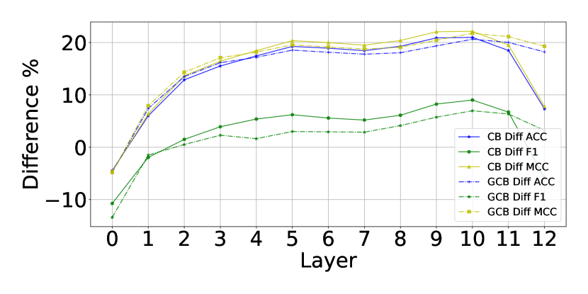
(c) Java250-Tagging-Diff.

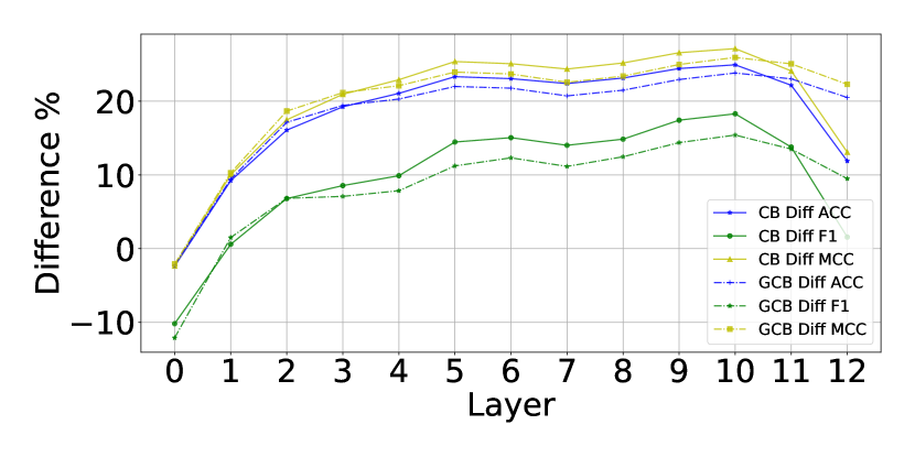
(d) POJ-104-Tagging-Diff.

Figure 10. Performance and Performance-Diff about Java250 and POJ-104 for Token tagging.

5.2. Semantic Analysis (RQ2)

More interestingly, we want to answer the extent to which CodeBERT and GraphCodeBERT encode code semantics.

5.2.1. Semantic Relation

The first two columns in Figure 11 show the probing performances for the representations from CodeBERT and GraphCodeBERT. When we check the probing performance about control dependence (Figure 11(a) and Figure 11(b)), control flow information (Figure 11(e) and Figure 11(f)) and data dependence (Figure 11(i) and Figure 11(j)), it can be seen that CodeBERT and GraphCodeBERT have the same ability to encode code semantics; the data flow input sequences to GraphCodeBERT do not make the representation encode more semantic information than CodeBERT. It is reasonable because MLM can help the model to learn semantics, as aforementioned Figure 1. The ability of MLM to learn code semantics is underestimated.

The last two columns in Figure 11 shows how pre-trained models get benefits from pre-training. The differences between GraphCodeBERT and GraphCodeBERT_rand are a little larger than the differences between CodeBERT and CodeBERT_rand in Figure 11(g), Figure 11(h) and Figure 11(k) in terms of MCC. However, in other cases and other metrics, the gains are not more than CodeBERT.

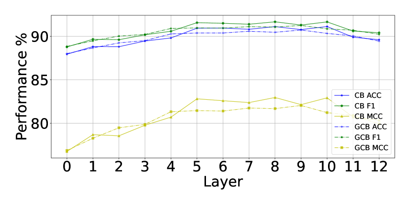
(a) Java250-CDG.

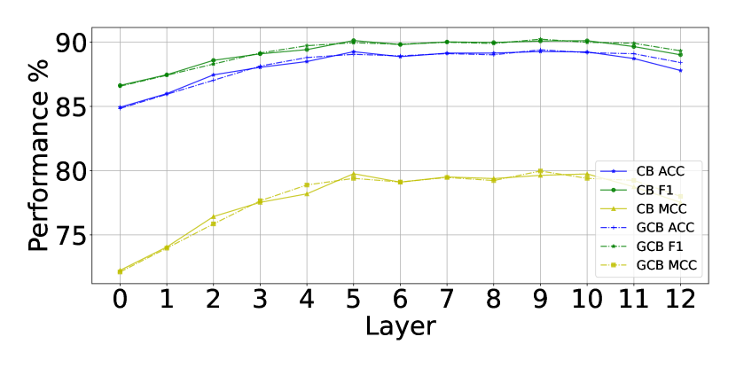
(b) POJ-104-CDG.

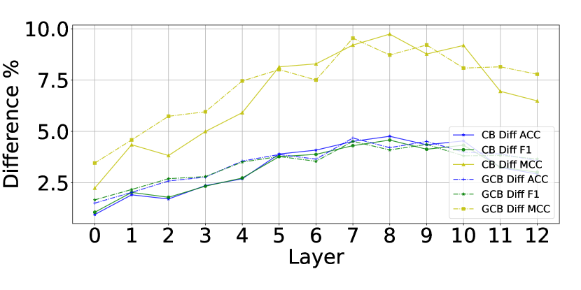
(c) Java250-CDG-Diff.

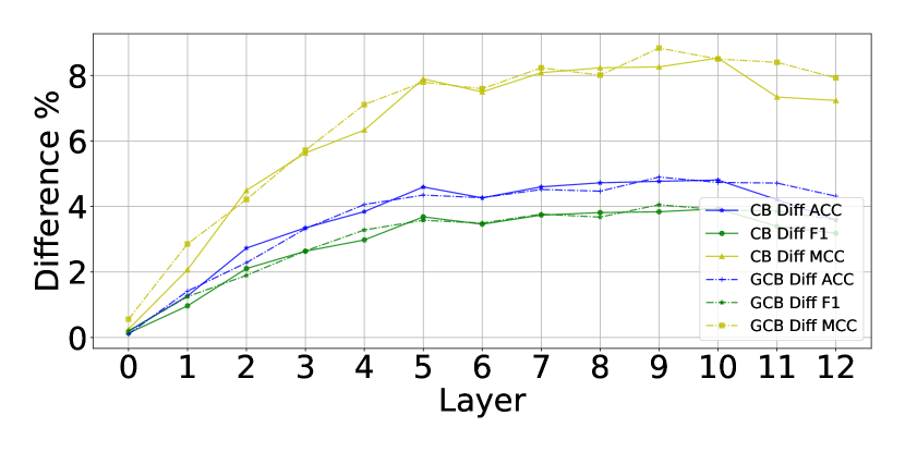
(d) POJ-104-CDG-Diff.

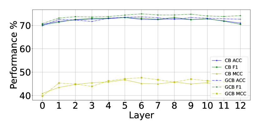
(e) Java250-CFG.

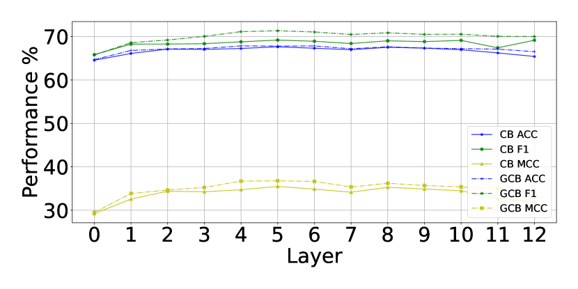
(f) POJ-104-CFG.

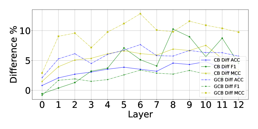
(g) Java250-CFG-Diff.

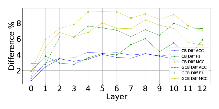
(h) POJ-104-CFG-Diff.

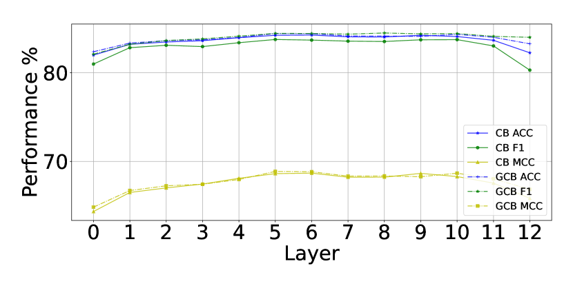
(i) Java250-DDG.

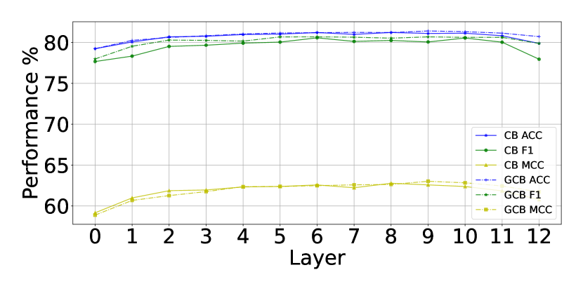
(j) POJ-104-DDG.

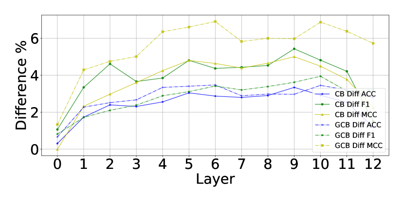
(k) Java250-DDG-Diff

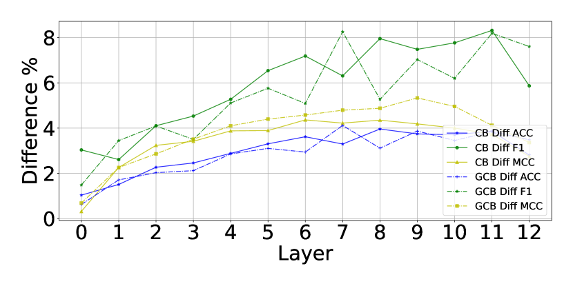
(l) POJ-104-DDG-Diff

Figure 11. Performance and Performance-Diff about Java250 and POJ-104 for Semantic Relation.

5.2.2. Semantic Propagation (inGraph)

The first two columns in Figure 12 demonstrate the probing performance for CodeBERT and GraphCodeBERT on the inGraph task. We can see that GraphCodeBERT is better than CodeBERT because almost all dashed lines are above the solid lines. The last two columns in Figure 12 show that pre-trained models can get gains from pre-training, and the benefits get larger with the deeper depth. In Figure 12(a), for control dependence on Java250, CodeBERT receives more benefits than GraphCodeBERT. In Figure 12(e), for data dependence on Java250, CodeBERT gets more gains than Graph CodeBERT after $Layer_{6}$. On POJ-104, both behave similarly.

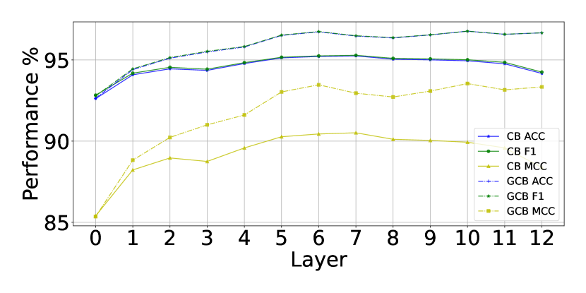
(a) Java250-CDG.

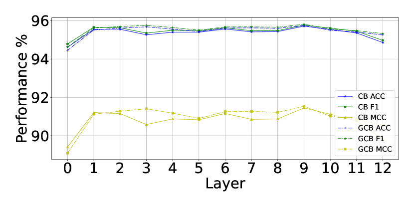
(b) POJ104-CDG.

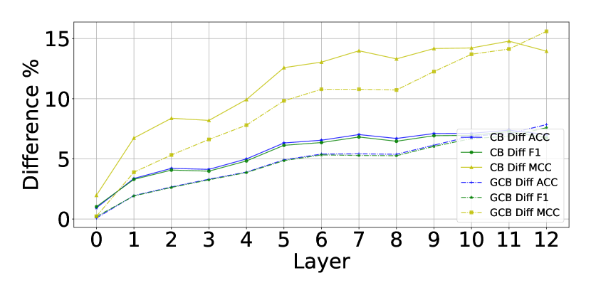
(c) Java250-CDG-Diff.

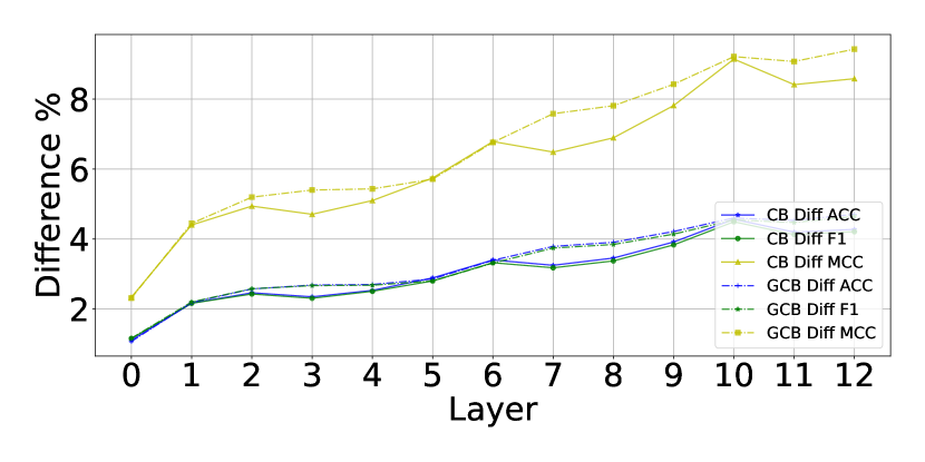
(d) POJ104-CDG-Diff.

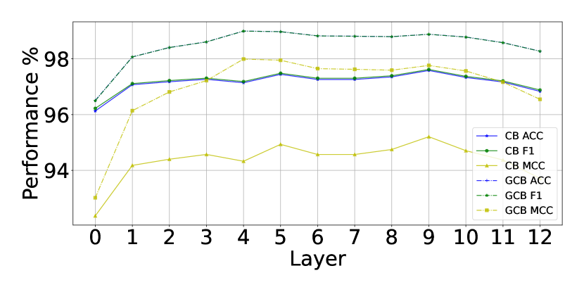
(e) Java250-DDG.

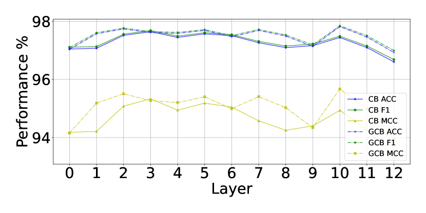
(f) POJ-104-DDG.

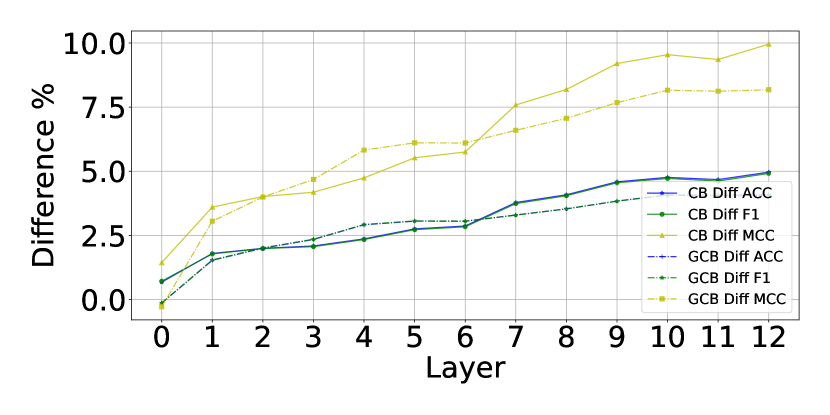
(g) Java250-DDG-Diff.

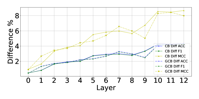
(h) POJ-104-DDG-Diff.

Figure 12. Performance and Performance-Diff about Java250 and POJ-104 for inGraph.

5.2.3. Type Inference

Figure 13(a) and Figure 13(b) illustrate the probing performance about type inference. We can see that GraphCodeBERT is a little better than CodeBERT. From the performance differences in Figure 13(c) and Figure 13(d), GraphCodeBERT gets more gains from pre-training than CodeBERT. The representations from the deeper layers have a stronger ability to infer one variable type.

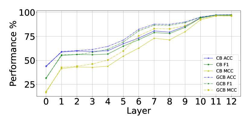
(a) Java250.

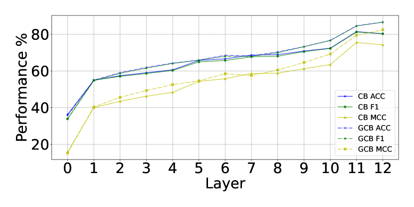
(b) POJ-104.

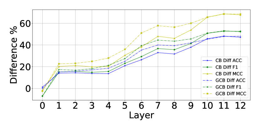
(c) Java250-Diff.

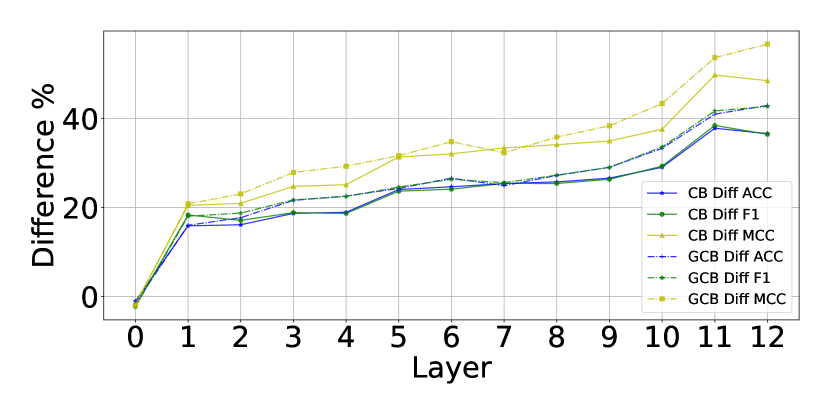
(d) POJ-104-Diff.

Figure 13. Performance Difference about Java250 and POJ-104 for Type Inference.

5.3. Performance Spearman Correlation

We observe that all performance curves seemly have the same trending for CodeBERT and GraphCodeBERT in Figure 9, Figure 10, Figure 11, Figure 12 and Figure 13. We compute Spearman Correlation with the permutation test between CodeBERT and GraphCodeBERT for probing performance, as shown in Table 4 on Java250/POJ104 for all tasks. Almost all correlations are more than 0.5, and the bold-font numbers mean that they have a p-value of $<1e-2$. The layer with the same index from CodeBERT and GraphCodeBERT has a consistent behaviour for encoding syntax and semantics.

Table 4. Spearman Correlation of Performance (bold-font means p-value $<1e-2$) between CodeBERT and GraphCodeBERT on all tasks, Java250/POJ-104

	F1	ACC	MCC
Syntax Node Pair	0.9341/0.9066	0.9615/0.9066	0.956/0.9066
Token Tagging	0.8462/0.978	0.8352/0.9176	0.8352/0.9286
SemanticDDG	0.8242/0.8242	0.9286/0.8736	0.9231/0.8187
SemanticCFG	0.4231/0.6813	0.4286/0.8776	0.522/0.9066
SemanticCDG	0.8022/0.9286	0.8116/0.9176	0.8022/0.9286
inGraphDDG	0.6484/0.6758	0.652/0.6758	0.6484/0.6758
inGraphCDG	0.5495/0.5769	0.522/0.6154	0.5495/0.5659
Type Infer	0.9890/0.9890	0.9890/0.9890	0.9890/0.9890

5.4. Attention Analysis (RQ3)

From the aforementioned analyses, we observe that CodeBERT and GraphCodeBERT well learn syntax and semantics about code. We investigate the roles of self-attention heads in learning code semantics using more than 10k semantic data. BERT-based models have $12\times 12$ attention heads. We use paired t-test to test our null hypothesis, i.e., $H_{0}:\mu_{d}=0$, there is no difference in the attention weights distributed among the semantically related tokens and non-semantically related tokens.

5.4.1. Layer-Level Analysis

For the layer-level test, the paired t-test results show that the statistic values are more significant than 15 and p-values are lower than $1e-2$ for all layers of both models on data dependence and control flow information. We can conclude that attention heads can encode the two types of semantic information well. However, not all the layers can encode control dependence well on the dataset Java250. For CodeBERT, there are only three layers $Layer_{4}$, $Layer_{6}$ and $Layer_{11}$ that can encode control dependence. For GraphCodeBERT, $Layer_{1}$, $Layer_{2}$ and $Layer_{3}$ fail to encode control dependence. The attention layers of CodeBERT and GraphCodeBERT can encode data dependence and control flow information well but should be improved for control dependence.

5.4.2. Head-Level Analysis

For the head-level analysis, we conduct the paired t-test for each attention head using the three semantic relationships, data dependence, control flow, and control dependence. First, we count the number of important heads with p-value $<1e-2$ and trivial heads with p-value $>1e-2$. Table 5 demonstrates the result. The numbers of important heads and non-important heads are denoted as importance/non-importance in Table 5. The first column is the semantic type. We can see that most heads in CodeBERT and GraphCodeBERT can encode data dependence and control flow well. For the different datasets, the overlapping number of important heads is very high as shown in the 4th column and the 7th column for CodeBERT and GraphCodeBERT, respectively. When we count the crossing-model overlapping, we find that CodeBERT and GraphCodeBERT share most of the important heads, as shown in the last two columns. However, when we see the important heads about control dependence, we find that both CodeBERT and GraphCodeBERT are not as good as the other two types, and all of them are less than 100. To give more details, we visualize the important heads that are not blank, as shown in Figure 14. The blank blocks are the attention heads with p-value $>-1e2$. The first two columns are about CodeBERT (CB) and the last two columns are about GraphCodeBERT (GCB). The X-axis is the layer index, and Y-axis is the attention head index. We can find that the attention heads from the same layer can behave differently; some can encode semantic information while others do not. Figure 14 clearly show that CodeBERT and GraphCodebert encode less control dependence than data dependence and control flow information.

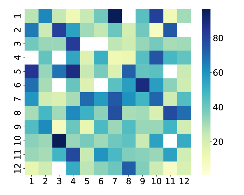
(a) Java-CB-DDG.

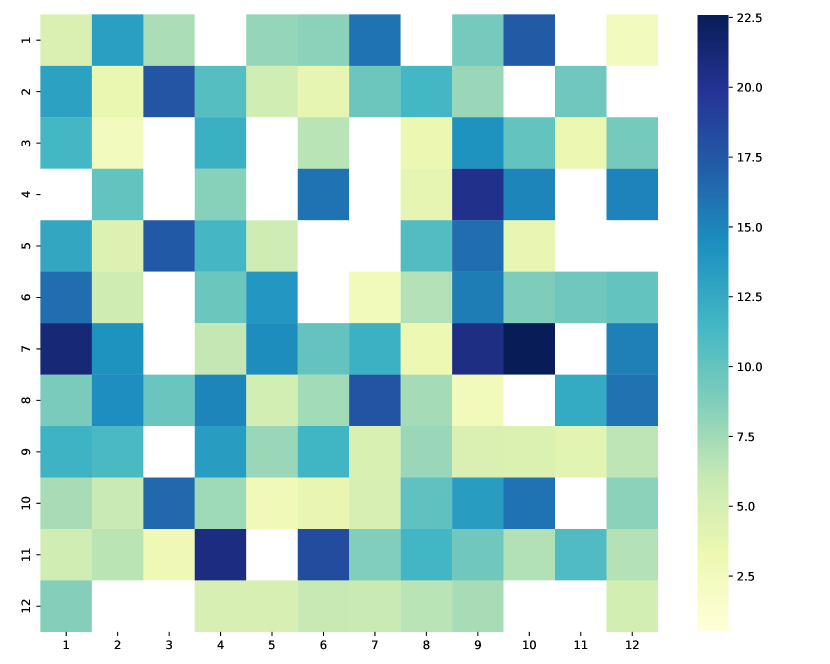
(b) POJ-CB-DDG.

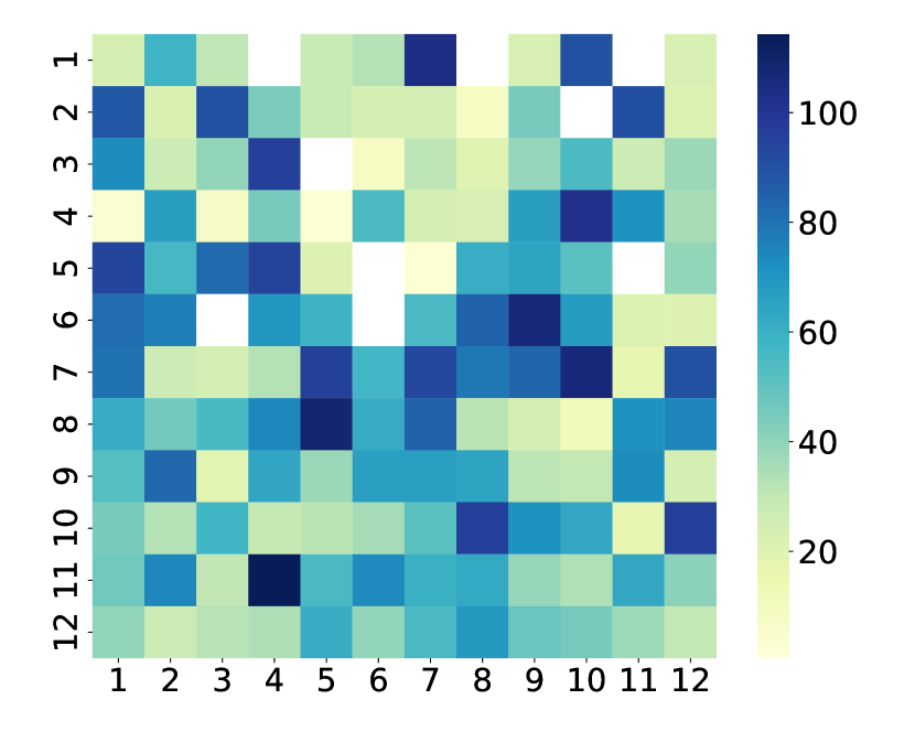
(c) Java-GCB-DDG.

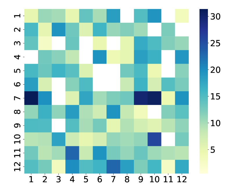
(d) POJ-GCB-DDG.

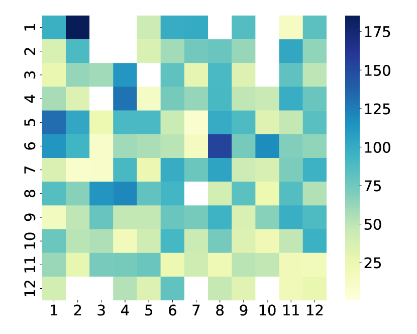
(e) Java-CB-CFG.

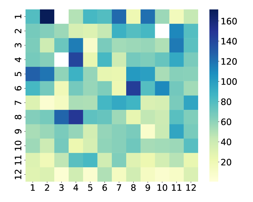
(f) POJ-CB-CFG.

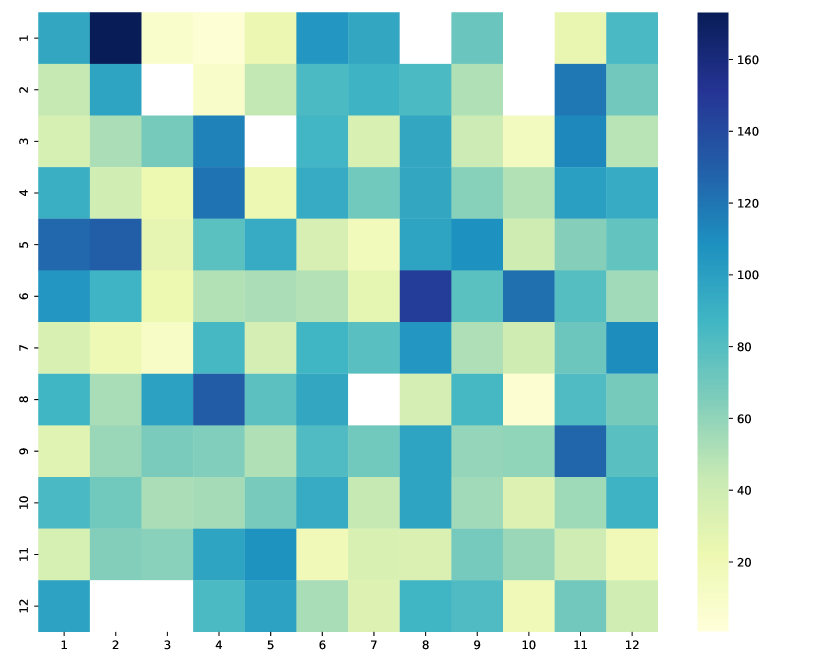
(g) Java-GCB-CFG.

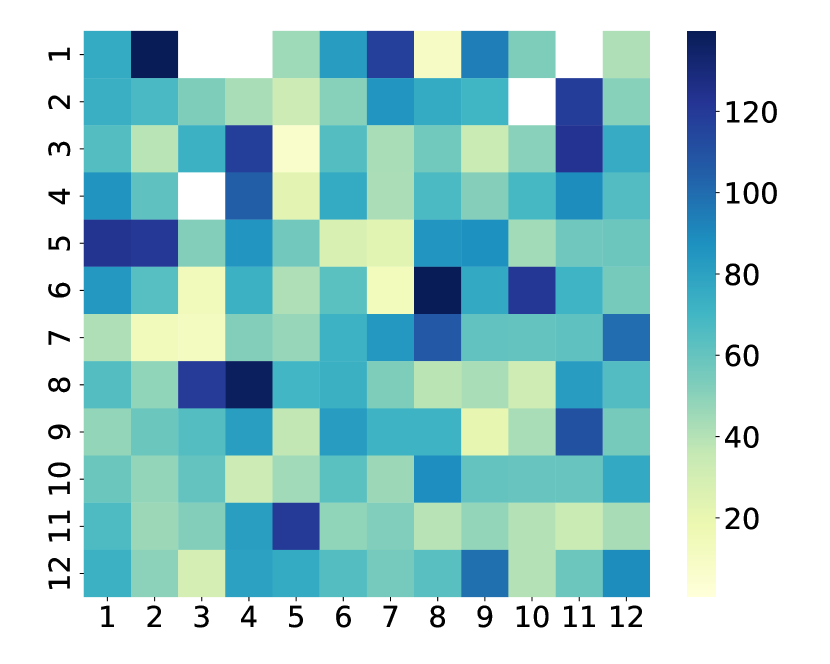
(h) POJ-GCB-CFG.

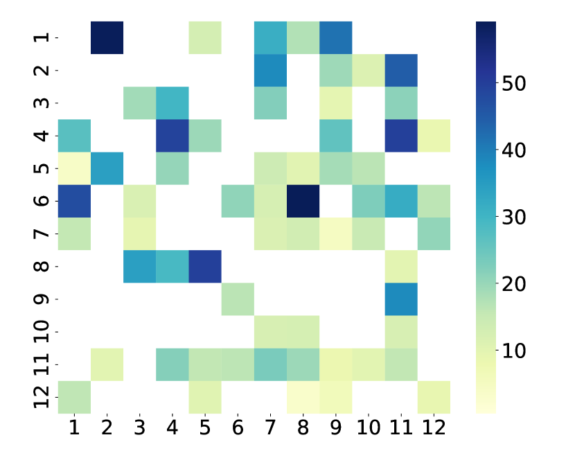
(i) Java-CB-CDG.

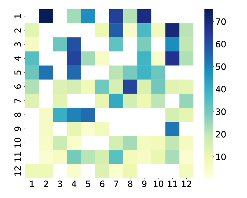
(j) POJ-CB-CDG.

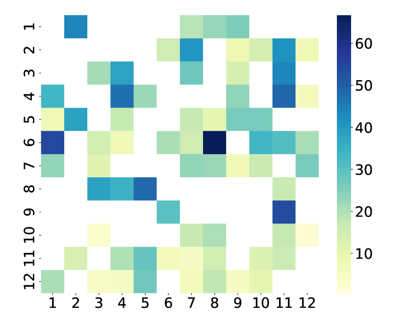
(k) Java-GCB-CDG.

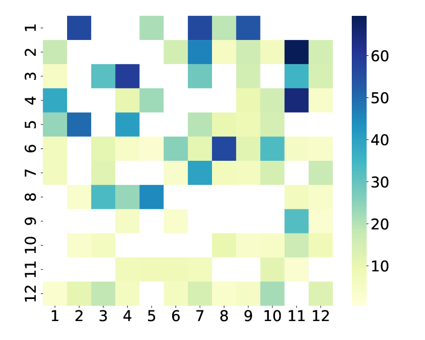
(l) POJ-GCB-CDG.

Figure 14. CodeBERT and GraphCodeBERT Paired T-Test for each attention head. X-axis is the layer index and Y-axis is the attention head index.

Table 5. Number of Heads Distribution for CodeBERT and GraphCodeBERT, Importance/Non-importance.

	CodeBERT			GraphCodeBERT			CodeBERT $\cap$ GraphCodeBERT
	Java250	POJ-104	$\cap$	Java250	POJ-104	$\cap$	Java250	POJ-104
DDG	133/11	115/29	114/10	135/9	124/20	123/8	129/5	114/19
CFG	129/15	141/3	129/3	136/8	139/5	132/1	129/8	139/3
CDG	65/79	93/51	63/49	71/73	86/58	67/54	62/70	82/47

6. Discussion

In this section, we first present the findings of our work, then detail the limitations and followed by introducing the threats to validity.

6.1. Findings and Limitations

In this work, we demonstrate that CodeBERT and GraphCodeBERT can encode syntax and semantic information while they behave differently for the different semantic types. To alleviate the conclusion bias due to the choice of performance metrics, we adopt three widely used metrics, Accuracy, F1 and MCC. For the syntax probing tasks, the performance curves of CodeBERT and GraphCodeBERT have the same trending and are pretty close. For the more challenging syntax task, token tagging, CodeBERT is slightly better than GraphCodeBERT at understanding the code grammar in terms of F1, while the other two metrics show that they are almost the same. There is a performance drop from $Layer_{11}$ to $Layer_{12}$, which needs future analysis. The final layer is not better than the middle layers for encoding the syntax information. This observation is consistent with López et al. (2022). More importantly, we illustrate that CodeBERT and GraphCodeBERT can encode code semantics well at the layer level from the three (3) semantic probing tasks and the layer-level head analysis. CodeBERT and GraphCodeBERT can encode control dependence but not better than data dependence and control flow. The Spearman correlation analysis shows that the roles of the layers with the same index from CodeBERT and GraphCodeBERT are almost similar in encoding syntax and semantics. The head-level attention analysis reveals that the different heads are different to learn syntax and semantics.

Our work has several limitations. First, our work includes two SOTA transformer-encoder models, CodeBERT and GraphCodeBERT. Both of them adopt the MLM pre-training strategy. The differences between GraphCodeBERT and CodeBERT are that 1) GraphCodeBERT uses the data flow sequence 2) GraphCodeBERT uses one larger pre-training dataset. We do not include the transformer-decoder or seq-seq code models. Second, the token tagging task is related to the specific programming language grammar rules, and the labels of the token tagging are different for the different programming languages. Third, we study how CodeBERT and GraphCodeBERT understand one function semantic because our static analysis is the intraprocedural analysis for each function code.

6.2. Threats to Validity

Internal validity is mainly about the implementation and the tools we use. For AST and static analysis, to build a high-quality dataset for analysis, we choose the tools that are used by many researchers to avoid mistakes in the data. We reuse the model code that is public and widely used by researchers. We choose the code datasets that are widely used. Construct validity is about if our probing analysis is true and not false positive. We use the default settings from the original papers and repeat all experiments multiple times.

External validity is about if our probing tasks can represent the syntax and semantics of the code. To solve this, we utilize Abstract Syntax Tree (AST) for syntax probing and statics analysis ( e.g., dependence graphs ) for semantics probing. By using them, we can make sure the probing data we use contain the syntax and semantics properties, respectively.

7. Related Work

In this section, we briefly introduce the pre-trained models for code as well as the probing analysis for code pre-trained models.

Pre-Trained Models for Code. According to the pre-training strategies and model architectures, we can group the pre-trained models into three (3) types: auto-encoding models, auto-regressive models, and sequence-to-sequence (Seq2Seq) models. Auto-encoding models utilize Transformer encoders and are pre-trained with objectives such as Masked Language Modelling (MLM). MLM masks some tokens in the code sequence and expects the model to predict the masked tokens using bidirectional context information, which in fact enables the model to use future tokens to predict current mask tokens. CodeBERT (Feng et al., 2020) is pre-trained on CodeSearchNet dataset (Husain et al., 2019). GraphCodeBERT (Guo et al., 2020) includes one additional input type, data flow sequence, compared with CodeBERT. CodeBERT and GraphCodeBERT use the encoder of Transformer. Auto-regressive models use Causal Language Modelling (CLM) to pre-train the transformers in a left-to-right manner. CodeGPT (Lu et al., 2021) uses this pre-training strategy and keeps the transformer decoder. Seq2Seq models, e.g., CodeT5 (Wang et al., 2021), use both an encoder and a decoder in the Transformer. CommitBART (Liu et al., 2022) uses BART architecture to pre-train a model for GitHub commits.

Probing Analysis for Code Pre-trained Models. Pre-trained models have been used to support many tasks due to their excellent generalization ability, especially BERT in natural language processing. The impressive performance of BERT stimulates loads of work trying to interpret and understand these newly invented large-scale blackbox models. These analysis works can help users understand and apply pre-trained models. Probing (Rogers et al., 2020; Conneau et al., 2018; Zhao et al., 2020) is one of the most prominent techniques widely leveraged for interpretability. Probing analysis aims at diagnosing which types of regularities are encoded in a representation extracted from data. The basis of probing is that if a simple classifier, e.g., a linear classifier, built upon the representations can solve a task sufficiently well, then the representations should contain informative features about the task already.

Recent works strive to analyze pre-trained code models via probing. Wan et al. (2022) evaluate if pre-trained models learn programming language syntax, and they measure the distance among node tokens at AST. López et al. (2022) analyze pre-trained models in a global-level AST by projecting AST into a subspace. Troshin and Chirkova (2022) develop a group of probing tasks to see if pre-trained models learn code syntax structure. The latest work (Shen et al., 2022) finds that pre-trained code models can learn code syntax but is not better than the rule-based methods. Karmakar and Robbes (2021) evaluate pre-trained models based on AST.

8. Conclusion and Future Work

In this work, we devise a group of probing tasks for code syntax and semantics. We extract the syntax and semantic relationships(facts) among tokens from AST and program analysis graphs. We assume that if code pre-trained models encode code syntax and semantics well, the probing classifier is able to infer these syntax and semantic facts from the vector representation of code models. For the syntax probing, we design two tasks 1). syntax node pair prediction, and 2). token tagging. For the semantic probing, we design three tasks based on the static analysis 1). semantic relationship prediction, 2). semantic propagation prediction, and 3) type inference. We check the layer-behaviour consistency between CodeBERT and GraphCodeBERT in terms of syntax and semantics via Spearman’s $\rho$. To give insights, we conduct statistical analysis about the attention heads for code semantics based on the facts without any learning process.

For future work, we plan to investigate how different model architectures affect code representation, e.g., seq2seq, transformer-decoder and graph neural networks. We also plan to study what is the best choice of pooling operations for downstream code tasks. In the end, we also want to study how pre-trained models change their representations after fine-tuning with the domain knowledge.

References

- (1)
- Aggarwal et al. (2001) Charu C. Aggarwal, Alexander Hinneburg, and Daniel A. Keim. 2001. On the Surprising Behavior of Distance Metrics in High Dimensional Spaces. In Proceedings of the 8th International Conference on Database Theory (ICDT ’01). Springer-Verlag, Berlin, Heidelberg, 420–434.
- Ahmad et al. (2021) Wasi Uddin Ahmad, Saikat Chakraborty, Baishakhi Ray, and Kai-Wei Chang. 2021. Unified pre-training for program understanding and generation. arXiv preprint arXiv:2103.06333 (2021).
- Allamanis et al. (2017) Miltiadis Allamanis, Marc Brockschmidt, and Mahmoud Khademi. 2017. Learning to represent programs with graphs. arXiv preprint arXiv:1711.00740 (2017).
- Buratti et al. (2020) Luca Buratti, Saurabh Pujar, Mihaela Bornea, Scott McCarley, Yunhui Zheng, Gaetano Rossiello, Alessandro Morari, Jim Laredo, Veronika Thost, Yufan Zhuang, et al. 2020. Exploring software naturalness through neural language models. arXiv preprint arXiv:2006.12641 (2020).
- Conneau et al. (2018) Alexis Conneau, German Kruszewski, Guillaume Lample, Loïc Barrault, and Marco Baroni. 2018. What you can cram into a single $&!#* vector: Probing sentence embeddings for linguistic properties. In Proceedings of the 56th Annual Meeting of the Association for Computational Linguistics (Volume 1: Long Papers). Association for Computational Linguistics, Melbourne, Australia, 2126–2136. https://doi.org/10.18653/v1/P18-1198
- Drain et al. (2021) Dawn Drain, Chen Wu, Alexey Svyatkovskiy, and Neel Sundaresan. 2021. Generating bug-fixes using pretrained transformers. In Proceedings of the 5th ACM SIGPLAN International Symposium on Machine Programming. 1–8.
- Feng et al. (2020) Zhangyin Feng, Daya Guo, Duyu Tang, Nan Duan, Xiaocheng Feng, Ming Gong, Linjun Shou, Bing Qin, Ting Liu, Daxin Jiang, et al. 2020. Codebert: A pre-trained model for programming and natural languages. arXiv preprint arXiv:2002.08155 (2020).
- Guo et al. (2020) Daya Guo, Shuo Ren, Shuai Lu, Zhangyin Feng, Duyu Tang, Shujie Liu, Long Zhou, Nan Duan, Alexey Svyatkovskiy, Shengyu Fu, et al. 2020. Graphcodebert: Pre-training code representations with data flow. arXiv preprint arXiv:2009.08366 (2020).
- Horwitz and Reps (1992) Susan Horwitz and Thomas Reps. 1992. The Use of Program Dependence Graphs in Software Engineering. In Proceedings of the 14th International Conference on Software Engineering (Melbourne, Australia) (ICSE ’92). Association for Computing Machinery, New York, NY, USA, 392–411. https://doi.org/10.1145/143062.143156
- Husain et al. (2019) Hamel Husain, Ho-Hsiang Wu, Tiferet Gazit, Miltiadis Allamanis, and Marc Brockschmidt. 2019. Codesearchnet challenge: Evaluating the state of semantic code search. arXiv preprint arXiv:1909.09436 (2019).
- Kanade et al. (2019) Aditya Kanade, Petros Maniatis, Gogul Balakrishnan, and Kensen Shi. 2019. Pre-trained contextual embedding of source code. (2019).
- Karampatsis and Sutton (2020) Rafael-Michael Karampatsis and Charles Sutton. 2020. Scelmo: Source code embeddings from language models. arXiv preprint arXiv:2004.13214 (2020).
- Karmakar and Robbes (2021) Anjan Karmakar and Romain Robbes. 2021. What do pre-trained code models know about code?. In 2021 36th IEEE/ACM International Conference on Automated Software Engineering (ASE). IEEE, 1332–1336.
- Li et al. (2022) Xueyang Li, Shangqing Liu, Ruitao Feng, Guozhu Meng, Xiaofei Xie, Kai Chen, and Yang Liu. 2022. TransRepair: Context-aware Program Repair for Compilation Errors. arXiv preprint arXiv:2210.03986 (2022).
- Li et al. (2015) Yujia Li, Daniel Tarlow, Marc Brockschmidt, and Richard Zemel. 2015. Gated graph sequence neural networks. arXiv preprint arXiv:1511.05493 (2015).
- Liu et al. (2019) Nelson F. Liu, Matt Gardner, Yonatan Belinkov, Matthew E. Peters, and Noah A. Smith. 2019. Linguistic Knowledge and Transferability of Contextual Representations. In Proceedings of the Conference of the North American Chapter of the Association for Computational Linguistics: Human Language Technologies.
- Liu et al. (2020) Shangqing Liu, Yu Chen, Xiaofei Xie, Jingkai Siow, and Yang Liu. 2020. Retrieval-augmented generation for code summarization via hybrid gnn. arXiv preprint arXiv:2006.05405 (2020).
- Liu et al. (2022) Shangqing Liu, Yanzhou Li, and Yang Liu. 2022. CommitBART: A Large Pre-trained Model for GitHub Commits. arXiv preprint arXiv:2208.08100 (2022).
- Liu et al. (2023) Shangqing Liu, Bozhi Wu, Xiaofei Xie, Guozhu Meng, and Yang Liu. 2023. ContraBERT: Enhancing Code Pre-trained Models via Contrastive Learning. arXiv preprint arXiv:2301.09072 (2023).
- López et al. (2022) José Antonio Hernández López, Martin Weyssow, Jesús Sánchez Cuadrado, and Houari Sahraoui. 2022. AST-Probe: Recovering abstract syntax trees from hidden representations of pre-trained language models. arXiv preprint arXiv:2206.11719 (2022).
- Lu et al. (2021) Shuai Lu, Daya Guo, Shuo Ren, Junjie Huang, Alexey Svyatkovskiy, Ambrosio Blanco, Colin Clement, Dawn Drain, Daxin Jiang, Duyu Tang, et al. 2021. Codexglue: A machine learning benchmark dataset for code understanding and generation. arXiv preprint arXiv:2102.04664 (2021).
- Mirkes et al. (2020) Evgeny M Mirkes, Jeza Allohibi, and Alexander Gorban. 2020. Fractional norms and quasinorms do not help to overcome the curse of dimensionality. Entropy 22, 10 (2020), 1105.
- Mou et al. (2016) Lili Mou, Ge Li, Lu Zhang, Tao Wang, and Zhi Jin. 2016. Convolutional neural networks over tree structures for programming language processing. In Proceedings of the Thirtieth AAAI Conference on Artificial Intelligence. 1287–1293.
- Puri et al. (2021) Ruchir Puri, David S Kung, Geert Janssen, Wei Zhang, Giacomo Domeniconi, Vladimir Zolotov, Julian Dolby, Jie Chen, Mihir Choudhury, Lindsey Decker, et al. 2021. CodeNet: A large-scale AI for code dataset for learning a diversity of coding tasks. arXiv preprint arXiv:2105.12655 (2021).
- Rogers et al. (2020) Anna Rogers, Olga Kovaleva, and Anna Rumshisky. 2020. A Primer in BERTology: What We Know About How BERT Works. Transactions of the Association for Computational Linguistics 8 (2020), 842–866. https://doi.org/10.1162/tacl_a_00349
- Shen et al. (2022) Da Shen, Xinyun Chen, Chenguang Wang, Koushik Sen, and Dawn Song. 2022. Benchmarking Language Models for Code Syntax Understanding. arXiv preprint arXiv:2210.14473 (2022).
- Svyatkovskiy et al. (2020) Alexey Svyatkovskiy, Shao Kun Deng, Shengyu Fu, and Neel Sundaresan. 2020. Intellicode compose: Code generation using transformer. In Proceedings of the 28th ACM Joint Meeting on European Software Engineering Conference and Symposium on the Foundations of Software Engineering. 1433–1443.
- Tenney et al. (2019) Ian Tenney, Patrick Xia, Berlin Chen, Alex Wang, Adam Poliak, R Thomas McCoy, Najoung Kim, Benjamin Van Durme, Samuel R Bowman, Dipanjan Das, et al. 2019. What do you learn from context? probing for sentence structure in contextualized word representations. arXiv preprint arXiv:1905.06316 (2019).
- Troshin and Chirkova (2022) Sergey Troshin and Nadezhda Chirkova. 2022. Probing Pretrained Models of Source Code. arXiv preprint arXiv:2202.08975 (2022).
- Vaswani et al. (2017) Ashish Vaswani, Noam Shazeer, Niki Parmar, Jakob Uszkoreit, Llion Jones, Aidan N Gomez, Łukasz Kaiser, and Illia Polosukhin. 2017. Attention is all you need. Advances in neural information processing systems 30 (2017).
- Wan et al. (2022) Yao Wan, Wei Zhao, Hongyu Zhang, Yulei Sui, Guandong Xu, and Hai Jin. 2022. What Do They Capture? A Structural Analysis of Pre-Trained Language Models for Source Code. In Proceedings of the 44th International Conference on Software Engineering (Pittsburgh, Pennsylvania) (ICSE ’22). Association for Computing Machinery, New York, NY, USA, 2377–2388. https://doi.org/10.1145/3510003.3510050
- Wang et al. (2021) Yue Wang, Weishi Wang, Shafiq Joty, and Steven CH Hoi. 2021. Codet5: Identifier-aware unified pre-trained encoder-decoder models for code understanding and generation. arXiv preprint arXiv:2109.00859 (2021).
- Zhao et al. (2020) Mengjie Zhao, Philipp Dufter, Yadollah Yaghoobzadeh, and Hinrich Schütze. 2020. Quantifying the Contextualization of Word Representations with Semantic Class Probing. In Findings of the Association for Computational Linguistics: EMNLP 2020. Association for Computational Linguistics, Online, 1219–1234. https://doi.org/10.18653/v1/2020.findings-emnlp.109
- Zhou et al. (2019) Yaqin Zhou, Shangqing Liu, Jingkai Siow, Xiaoning Du, and Yang Liu. 2019. Devign: Effective vulnerability identification by learning comprehensive program semantics via graph neural networks. In Advances in Neural Information Processing Systems. 10197–10207.