Isothermal and isentropic speed of sound in (2+1)-flavor QCD at non-zero baryon chemical potential

Abstract

Recently interest in calculations of the speed of sound in QCD under conditions like constant temperature $c^{2}_{T}$ or constant entropy per net baryon number $c^{2}_{s}$ arose in the discussion of experimental results coming from heavy ion experiments. It has been stressed that the former in particular is closely related to higher order cumulants of conserved charge fluctuations that are calculated in lattice QCD. We present here results on $c^{2}_{T}$ and $c^{2}_{s}$ and compare results at vanishing strangeness chemical potential and vanishing net strangeness number with hadron resonance gas model calculations. We stress the difference of both observables at low temperature arising from the light meson sector, which does not contribute to $c^{2}_{T}$.

1 Introduction

The isentropic speed of sound and isothermal speeds of sound are given by, respectively,

$$c_{s}^{2}=\left(\partialderivative{p}{\epsilon}\right)_{s/n_{B}}~{}~{}~{}~{}~{}\text{and}~{}~{}~{}~{}~{}c_{T}^{2}=\left(\partialderivative{p}{\epsilon}\right)_{T},$$ (1)

where $p$ is the pressure, $\epsilon$ is the energy density, $s$ is the entropy density, $n_{B}$ is the net baryon-number density, and $T$ is the temperature. It is one of many bulk thermodynamic observables useful for characterizing strongly interacting matter. For instance in the simple Bjorken flow model, assuming a constant $c_{s}^{2}$, one can show [1] that the energy density will decrease with proper time $\tau$ as $\tau^{-(1+c_{s}^{2})}$. In the context of heavy ion collisions (HIC), the system cools with longitudinal expansion of the fireball according to $c_{s}^{2}$ in this picture. Also in the context of HIC, it can be used to look out for a long-lived fireball, which may coincide with a softest point where the pressure-to-energy-density ratio, and hence $c_{s}^{2}$, attains a minimum [2]. The isothermal speed of sound may also be of interest in the context of HIC, as a new method to estimate $c_{T}^{2}$ in HIC has been recently suggested in Ref. [3]. In the context of neutron stars, $c_{s}^{2}$ is interesting since the relationship between the star masses and radii is influenced by how $c_{s}^{2}$ changes with $n_{B}$ [4]. This context is particularly interesting, since some situations may suggest or require $c_{s}^{2}$ exceed its conformal limit $1/3$ [5, 6, 7].

With these applications in mind, it is worthwhile to revisit lattice investigations of the speed of sound. The speed of sound has been extensively studied at $\mu_{B}=0$ on the lattice [8, 9, 10]. Here we extend these results to obtain a first calculation of $c_{s}^{2}$ at finite baryon, electric charge, and strangeness chemical potentials $\mu_{B}$, $\mu_{Q}$, and $\mu_{S}$ on the lattice. In order to obtain observables that are functions of $\mu_{B}$ and $T$ only, and in order to target physics of interest to HIC, we introduce two constraints

$$n_{S}=0~{}~{}~{}~{}~{}~{}~{}\text{and}~{}~{}~{}~{}~{}~{}~{}n_{Q}/n_{B}=r,$$ (2)

where $n_{S}$ and $n_{Q}$ are the net strangeness and electric charge densities, and $r=0.4$ or $0.5$ corresponding respectively to collisions at the Relativistic Heavy Ion Collider (RHIC) and the isospin-symmetric case.

Thermodynamic observables including $c_{s}^{2}$ calculated at $r=0.5$ have been studied extensively by us in a recent publication [11]. This extends previous $6{}^{\rm th}$-order results [12] up to $8{}^{\rm th}$-order in the pressure series. In these proceedings, we supplement our most recent results with a calculation of $c_{T}^{2}$ at $\mu_{Q}=\mu_{Q}=0$ and extend speed of sound results on lines of constant $s/n_{B}$ to include $r=0.4$, which is similar to the RHIC scenario. We confirm that differences in $c_{s}^{2}$ and lines of constant $s/n_{B}$ arising from this change in $r$ are negligible. For $c_{T}^{2}$, we will introduce instead the constraint $\mu_{Q}=\mu_{S}=0$. While less directly relevant to HIC, this situation has $\mu_{Q}=0$ in common with $r=0.5$ and has the advantage of especially simple expressions for $c_{T}^{2}$.

2 Strategy of calculations

The general strategy starts with finding $p$. Once we have $p$, we can derive all other quantities from basic thermodynamic relations. For temperatures near and above $T_{\rm pc}$ we use lattice QCD; near and below $T_{\rm pc}$ we use the hadron resonance gas (HRG) model.

2.1 Lattice QCD

For convenience, we introduce dimensionless variables $\hat{X}\equiv XT^{-k}$ with $k\in\mathbb{Z}$ chosen such that $\hat{X}$ is dimensionless. Thermodynamic observables are determined using the Taylor expansion approach, i.e. we expand

$$\hat{p}=\frac{1}{VT^{3}}\log\mathcal{Z}_{\rm QCD}(T,V,\hat{\mu}_{B},\hat{\mu}_{Q},\hat{\mu}_{S})=\sum_{i,j,k=0}^{\infty}\frac{\chi_{ijk}^{BQS}}{i!j!k!}\hat{\mu}_{B}^{i}\hat{\mu}_{Q}^{j}\hat{\mu}_{S}^{k},$$ (3)

with expansion coefficients

$$\chi_{ijk}^{BQS}\equiv\chi_{ijk}^{BQS}(T)=\frac{\partial\hat{p}}{\partial\hat{\mu}_{B}^{i}\partial\hat{\mu}_{Q}^{j}\partial\hat{\mu}_{S}^{k}}\;\Bigg{|}_{\hat{\mu}=0}.$$ (4)

Imposing our constraints (2) renders $\hat{\mu}_{Q}$ and $\hat{\mu}_{S}$ functions of $\hat{\mu}_{B}$ and $T$, and hence we can reorganize  $\hat{p}$ as

$$\hat{p}=P_{0}+\sum_{k=1}^{\infty}P_{2k}(T)\hat{\mu}_{B}^{2k}$$ (5)

For more details on our implementation of constraints, see e.g. Ref. [15, 14, 11].

Perhaps the most straightforward strategy to obtain $c_{s}^{2}$ on the lattice, and the one that we employ here, is to use

$$c_{s}^{2}\equiv c^{2}_{\vec{X}}=\left(\frac{\partial p}{\partial\epsilon}\right)_{\vec{X}}=\frac{\left(\partial p/\partial T\right)_{\vec{X}}}{\left(\partial\epsilon/\partial T\right)_{\vec{X}}},$$ (6)

where $\vec{X}\equiv(s/n_{B},r,n_{S})$. In this strategy, one takes numerical $T$-derivatives of $p(T)$ and $\epsilon(T)$ that were determined along the line of constant physics $\vec{X}$.

When $T$ is held fixed, one can proceed analytically a bit further in a relatively straightforward manner through Taylor expansion. In particular one has in this case

$$c_{T}^{2}=\left(\frac{\partial p}{\partial\epsilon}\right)_{T}=\left(\frac{\partial p}{\partial\hat{\mu}_{B}}\right)\left(\frac{\partial\epsilon}{\partial\hat{\mu}_{B}}\right)^{-1}.$$ (7)

When $\hat{\mu}_{Q}=\hat{\mu}_{S}=0$, the relationship between Taylor coefficients of $\hat{p}$ and $\hat{\epsilon}$ become especially simple, and one eventually finds

$$c_{T}^{-2}-3=\frac{2P^{\prime}_{2}\hat{\mu}_{B}+4P^{\prime}_{4}\hat{\mu}_{B}^{3}+\order{\hat{\mu}_{B}^{5}}}{2P_{2}\hat{\mu}_{B}+4P_{4}\hat{\mu}_{B}^{3}+\order{\hat{\mu}_{B}^{5}}}~{}~{}~{}~{}~{}~{}\text{or}~{}~{}~{}~{}~{}~{}c_{T}^{-2}=3+\frac{P^{\prime}_{2}}{P_{2}}+\sum_{k}c_{T,2k}\hat{\mu}_{B}^{2k}.$$ (8)

Using the notation $X^{\prime}=T{\rm dX}/{\rm d}T$, we get for the expansion coefficients

$$c_{T,2}=\left(\frac{P_{4}}{P_{2}}\right)^{\prime},~{}~{}~{}~{}c_{T,4}=4\left(\frac{P_{4}}{P_{2}}\right)\left(\frac{P_{4}}{P_{2}}\right)^{\prime}+3\left(\frac{P_{6}}{P_{2}}\right)^{\prime},~{}~{}~{}~{}...$$ (9)

2.2 Hadron resonance gas

In the HRG model, we work in a phase where quarks are confined so that the only degrees of freedom are hadronic bound states. Hence this model is expected to be valid up to roughly $T_{\rm pc}$. A non-interacting, quantum, relativistic gas eventually delivers for particle species $i$

$$\frac{p_{i}}{T}=\frac{m_{i}^{2}g_{i}T}{2\pi^{2}}\sum_{k=1}^{\infty}\frac{\eta_{i}^{k+1}z_{i}^{k}}{k^{2}}K_{2}\left(\frac{m_{i}k}{T}\right),~{}~{}~{}~{}~{}~{}~{}~{}z_{i}\equiv e^{\,\hat{\mu}_{B}B_{i}+\hat{\mu}_{Q}Q_{i}+\hat{\mu}_{S}S_{i}},$$ (10)

where $m_{i}$ is the species’ mass, $g_{i}$ is its degeneracy factor, $\eta_{i}=\pm 1$ for boson/fermion statistics, and $K_{2}$ is the modified Bessel function of the $2{}^{\rm nd}$ kind. The total $p$ is then found by summing over all known states.

In the special case $\hat{\mu}_{Q}=\hat{\mu}_{S}=0$, one can derive a relatively simple form for the isothermal speed of sound. This case is instructive to get some intuition about how the speed of sound behaves, especially at low temperatures, and it moreover shares $\hat{\mu}_{Q}=0$ in common with the $r=0.5$ case. One schematically has in this situation

$$\hat{p} =f_{M}(T)+f_{B}(T)\cosh(\hat{\mu}_{B}),$$ (11)

$$\hat{\epsilon} =3f_{M}(T)+f^{\prime}_{M}(T)+\left(3f_{B}(T)+f^{\prime}_{B}(T)\right)\cosh(\hat{\mu}_{B}),$$

where $f_{M}(T)$ and $f_{B}(T)$ are the mesonic and baryonic contributions, respectively. Hence when taking a $\hat{\mu}_{B}$-derivative, $f_{M}$ drops out. This makes computing the isothermal speed of sound especially straightforward:

$$c_{T}^{2}=\left(\frac{\partial p}{\partial\hat{\mu}_{B}}\right)\left(\frac{\partial\epsilon}{\partial\hat{\mu}_{B}}\right)^{-1}=\frac{1}{3+f^{\prime}_{B}(T)/f_{B}(T)},$$ (12)

i.e. in an HRG, $c_{T}^{2}$ will be $\hat{\mu}_{B}$-independent. This is in agreement with the $r=0.5$ expansion coefficients of $c_{T}^{2}$ given in eq. (9). To see this, note that for an HRG in the Boltzmann approximation, the expansion coefficients $P_{2k}$ are given by

$$P_{2k}=\frac{f_{B}(T)}{2k!}.$$ (13)

The ratios $P_{2k}/P_{2}$ are thus $T$-independent, which means the coefficients in eq. (9) vanish when applied to a $\hat{\mu}_{Q}=\hat{\mu}_{S}=0$ HRG.

To determine $c_{s}^{2}$ in HRG, one could use eq. (6). While this is quite successful for large $s/n_{B}$, which corresponds to small $\hat{\mu}_{B}$, we found it had numerical difficulties for $s/n_{B}\lesssim 10$. Instead, we use here Appendix C of Ref. [11], which while more elaborate to implement, increases numerical stability by circumventing the numerical $T$-derivatives. We find exact agreement between both approaches for $s/n_{B}\gtrsim 400$, while the second approach allows us to compute $c_{s}^{2}$ for $s/n_{B}\lesssim 10$ more reliably.

3 Computational setup

We use high-statistics data sets for $(2+1)$-flavor QCD with degenerate light quark masses $m_{u}=m_{d}\equiv m_{l}$ and a heavier strange quark mass $m_{s}$. These data sets were generated with the HISQ action using SIMULATeQCD [17] and have been presented in previous HotQCD studies [12, 13].

For $T<180$ MeV, the speed of sound is extracted from continuum-extrapolated data from $N_{\tau}=8$, $12$, and $16$ lattices with $m_{s}/m_{l}=27$, which is the physical value. For $T>180$ MeV, we use data [12] with slightly heavier light quarks, $m_{s}/m_{l}=20$. In all cases results have been obtained on lattices with aspect ratio $N_{\sigma}/N_{\tau}=4$.

We are often interested in the behavior of observables near the pseudocritical temperature $T_{\rm pc}$. When indicated on figures, we take $T_{\rm pc}=156.5(1.5)$ MeV from Ref. [19]. $T_{\rm pc}(\hat{\mu}_{B})$ curves use the $\order{\hat{\mu}_{B}^{2}}$ expansion

$$T_{\rm pc}(\hat{\mu}_{B})=T_{\rm pc}(0)\left(1-\kappa_{2}^{B}\hat{\mu}_{B}^{2}+\order{\hat{\mu}_{B}^{4}}\right)$$ (14)

using curvature coefficient $\kappa_{2}^{B}=0.016$ for $r=0.5$ and $\kappa_{2}^{B}=0.012$ for $r=0.4$.

The AnalysisToolbox [20] is used to facilitate HRG calculations and bootstrapping. Statistical uncertainty in all figures is represented by bands and is calculated through bootstrap resampling, unless otherwise stated. Central values are returned as the median, with the lower and upper error bounds given by the 32% and 68% quantiles, respectively. If needed, spline interpolations are cubic with evenly spaced knots, and temperature derivatives of lattice QCD data are calculated by fitting the temperature dependence with a spline, then calculating the derivative of the spline numerically.

4 Results

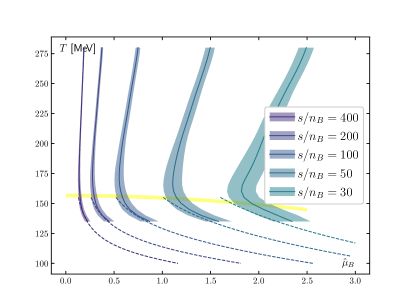
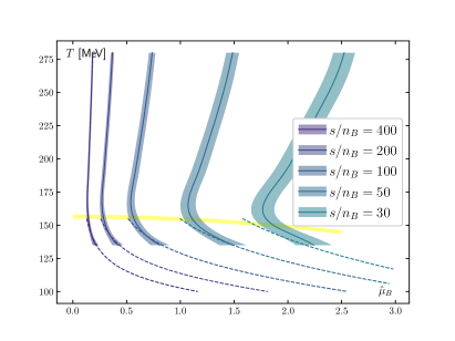
Figure 1: Lines of constant entropy per baryon number in the $T$-$\hat{\mu}_{B}$ plane for $r=0.4$ (left) and $r=0.5$ (right). Solid bands indicate results obtained by numerically solving $s/n_{B}$ derived from the $\order{\hat{\mu}_{B}^{6}}$ pressure series for $\hat{\mu}_{B}$. Dashed lines indicate QMHRG2020 model calculations. The yellow band indicates $T_{\rm pc}(\hat{\mu}_{B})$.

Results for $c_{s}^{2}$ are computed along lines of constant $s/n_{B}$, which are depicted for both the $r=0.4$ and $r=0.5$ cases in Fig. 1. We examine $400\leq s/n_{B}\leq 30$, which very roughly corresponds to the $s/n_{B}$ range covered by BES-II at RHIC for beam energies $7.7~{}{\rm GeV}\lesssim\sqrt{s_{{}_{NN}}}\lesssim 200~{}{\rm GeV}$. We find good agreement with HRG below $T_{\rm pc}$. For Figs. 1, 2, and 3, the behavior between the $r=0.4$ and $r=0.5$ cases is qualitatively the same and quantitatively very close, i.e. we verify that differences in these observables due to deviations from the isospin-symmetric case are quite small. Error bars for the $r=0.4$ case may be larger, since one introduces an error in $\hat{\mu}_{Q}(\hat{\mu}_{B})$, which is otherwise exactly zero in the $r=0.5$ case.

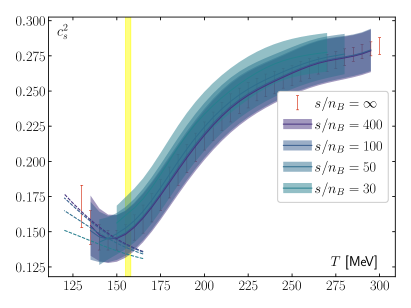
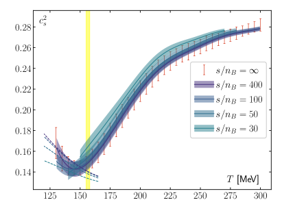
Figure 2: Isentropic speed of sound versus temperature for strangeness-neutral matter with $r=0.4$ (left) and $r=0.5$ (right). Dashed lines at low temperatures indicate QMHRG2020 model calculations, while the yellow band indicates $T_{\rm pc}$. $s/n_{B}=\infty$ data taken from Ref. [9].

In Fig. 2 we show our results for $c_{s}^{2}$ against $T$ for both $r=0.4$ and $r=0.5$. Fig. 3 shows the HRG results down to about $T=20$ MeV. In general one finds only mild quantitative differences with changing $s/n_{B}$ above $T_{\rm pc}$. We find good agreement between lattice results and HRG below $T_{\rm pc}$. Near $T_{\rm pc}$, one finds a dip in the lattice data for $s/n_{B}\geq 100$. Using both lattice and HRG results, one expects a dip also down to at least $s/n_{B}=30$. This dip location roughly corresponds to the location of the $p/\epsilon$ minimum, i.e. the softest point mentioned in the introduction, which one can also verify directly using our $p$ and $\epsilon$ data [11]. This gives yet another indication of the existence of a crossover at all chemical potentials examined in this study.

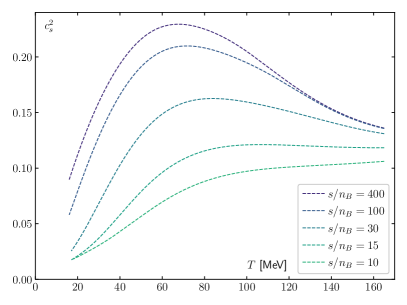
Figure 3: Isentropic speed of sound versus temperature for strangeness-neutral matter with $r=0.4$ (left) and $r=0.5$ (right) from QMHRG2020 model calculations.

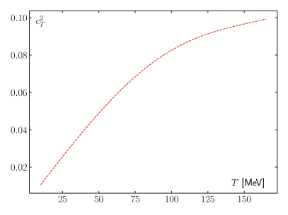
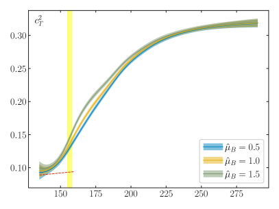
Figure 4: Isothermal speed of sound for strangeness-neutral matter. Left: QMHRG2020 calculation at $\hat{\mu}_{Q}=\hat{\mu}_{s}=0$. Right: Lattice data at $r=0.5$. Error bands come from error propagation. The yellow band indicates $T_{\rm pc}$, and the red, dashed line indicates the HRG curve from the left figure.

Turning to the QMHRG2020 results shown in Fig. 3, we see a peak in $c_{s}^{2}$ that decreases with decreasing $s/n_{B}$. Somewhere in the vicinity $s/n_{B}\in[10,15]$, the peak has vanished, and $c_{s}^{2}$ increases monotonically with $T$ up to 165 MeV. The $c_{s}^{2}$ curves at $r=0.4$ and $r=0.5$ seem to approach $c_{T}^{2}$ as $s/n_{B}\to 0$ with particularly close agreement at the lowest calculated $T$. We reiterate that we only have $c_{T}^{2}$ data at $\hat{\mu}_{Q}=\hat{\mu}_{S}=0$, which is a somewhat different situation than both $r=0.4$ and $r=0.5$. This precludes an unambiguous direct comparison.

From eq. (11) and (12) we see that $c_{T}^{2}$ is insensitive to mesons. We will use this as a starting point to understand the weakening of the peak in $c_{s}^{2}$. In the massless limit, one expects from eq. (10) that $c_{s}^{2}$ and $c_{T}^{2}$ will be 1/3 at all $T$. Continuing this behavior to small $m$, one expects that small masses have the tendency to pull speed of sound curves up toward 1/3. The isentropic speed of sound, which feels the mesonic sector, but should approach 0 at low $T$, therefore develops a peak. By contrast $c_{T}^{2}$ at $\hat{\mu}_{Q}=\hat{\mu}_{S}=0$ is insensitive to mesons, so it has no tendency to be pulled to 1/3. In Fig. 4 (right), we show a lattice determination of $c_{T}^{2}$ at $r=0.5$ using eq. (8). Despite the slight difference in external conditions, it agrees well with HRG at low $T$, and it rapidly approaches the ideal gas limit 1/3 at high $T$.

As a closing remark, we mention that our results for the speed of sound are in rough qualitative agreement with various model calculations, for instance PNJL and NJL models [21, 22, 23, 24, 25]; the quark-meson coupling model [26, 27]; the field correlator method [28, 29]; and the quasiparticle method [30].

5 Conclusion and outlook

We presented a first lattice calculation of $c_{s}^{2}$ and $c_{T}^{2}$ at finite chemical potential. The dip in $c_{s}^{2}$ near $T_{\rm pc}$, or equivalently its peak at lower $T$, can be understood through its sensitivity to light meson states. For all results we find a negligible difference between $r=0.4$ and $r=0.5$. Our results for $c_{s}^{2}$ are qualitatively in agreement with model calculations. Finally we note that the strategy of Appendix C in Ref. [11] works quite successfully for $c_{s}^{2}$, and hope to extend it to other thermodynamic observables.

References

- [1] J. D. Bjorken, Highly Relativistic Nucleus-Nucleus Collisions: The Central Rapidity Region, Phys. Rev. D 27 (1983) 140.
- [2] C. M. Hung and E. V. Shuryak, Hydrodynamics near the QCD phase transition: Looking for the longest lived fireball, Phys. Rev. Lett. 75 (1995) 4003 [hep-ph/9412360].
- [3] A. Sorensen, D. Oliinychenko, V. Koch and L. McLerran, Speed of Sound and Baryon Cumulants in Heavy-Ion Collisions, Phys. Rev. Lett. 127 (2021) 042303 [2103.07365].
- [4] F. Özel and P. Freire, Masses, Radii, and the Equation of State of Neutron Stars, Ann. Rev. Astron. Astrophys. 54 (2016) 401 [1603.02698].
- [5] L. McLerran and S. Reddy, Quarkyonic Matter and Neutron Stars, Phys. Rev. Lett. 122 (2019) 122701 [1811.12503].
- [6] C. Drischler, S. Han, J. M. Lattimer, M. Prakash, S. Reddy and T. Zhao, Limiting masses and radii of neutron stars and their implications, Phys. Rev. C 103 (2021) 045808 [2009.06441].
- [7] Y. Fujimoto, K. Fukushima, L. D. McLerran and M. Praszalowicz, Trace anomaly as signature of conformality in neutron stars, 2207.06753.
- [8] S. Borsanyi, G. Endrodi, Z. Fodor, A. Jakovac, S. D. Katz, S. Krieg et al., The QCD equation of state with dynamical quarks, JHEP 11 (2010) 077 [1007.2580].
- [9] HotQCD collaboration, Equation of state in ( 2+1 )-flavor QCD, Phys. Rev. D 90 (2014) 094503 [1407.6387].
- [10] S. Borsanyi, Z. Fodor, C. Hoelbling, S. D. Katz, S. Krieg and K. K. Szabo, Full result for the QCD equation of state with 2+1 flavors, Phys. Lett. B 730 (2014) 99 [1309.5258].
- [11] D. Bollweg, D. A. Clarke, J. Goswami, O. Kaczmarek, F. Karsch, S. Mukherjee et al., Equation of state and speed of sound of (2+1)-flavor QCD in strangeness-neutral matter at non-vanishing net baryon-number density, 2212.09043.
- [12] A. Bazavov et al., The QCD Equation of State to from Lattice QCD, Phys. Rev. D 95 (2017) 054504 [1701.04325].
- [13] HotQCD collaboration, Taylor expansions and Padé approximants for cumulants of conserved charge fluctuations at nonvanishing chemical potentials, Phys. Rev. D 105 (2022) 074511 [2202.09184].
- [14] J. Goswami, The isentropic equation of state of (2+1)-flavor qcd: An update based on high precision taylor expansion and padé-resummed expansion at finite chemical potentials, PoS LATTICE2022 (2022) 149 [2212.10016].
- [15] HotQCD collaboration, Skewness, kurtosis, and the fifth and sixth order cumulants of net baryon-number distributions from lattice QCD confront high-statistics STAR data, Phys. Rev. D 101 (2020) 074502 [2001.08530].
- [16] HotQCD collaboration, Second order cumulants of conserved charge fluctuations revisited: Vanishing chemical potentials, Phys. Rev. D 104 (2021) [2107.10011].
- [17] D. Bollweg, L. Altenkort, D. A. Clarke, O. Kaczmarek, L. Mazur, C. Schmidt et al., HotQCD on multi-GPU Systems, PoS LATTICE2021 (2022) 196 [2111.10354].
- [18] HotQCD collaboration, The chiral and deconfinement aspects of the QCD transition, Phys. Rev. D 85 (2012) 054503 [1111.1710].
- [19] HotQCD collaboration, Chiral crossover in QCD at zero and non-zero chemical potentials, Phys. Lett. B 795 (2019) 15 [1812.08235].
- [20] “AnalysisToolbox: A set of Python tools for analyzing physics data, in particular targeting lattice QCD.” https://github.com/LatticeQCD/AnalysisToolbox.
- [21] S. K. Ghosh, T. K. Mukherjee, M. G. Mustafa and R. Ray, Susceptibilities and speed of sound from PNJL model, Phys. Rev. D 73 (2006) 114007 [hep-ph/0603050].
- [22] R. Marty, E. Bratkovskaya, W. Cassing, J. Aichelin and H. Berrehrah, Transport coefficients from the Nambu-Jona-Lasinio model for , Phys. Rev. C 88 (2013) 045204 [1305.7180].
- [23] P. Deb, G. P. Kadam and H. Mishra, Estimating transport coefficients in hot and dense quark matter, Phys. Rev. D 94 (2016) 094002 [1603.01952].
- [24] M. Motta, R. Stiele, W. M. Alberico and A. Beraudo, Isentropic evolution of the matter in heavy-ion collisions and the search for the critical endpoint, Eur. Phys. J. C 80 (2020) 770 [2003.04734].
- [25] Y.-P. Zhao, Thermodynamic properties and transport coefficients of QCD matter within the nonextensive Polyakov–Nambu–Jona-Lasinio model, Phys. Rev. D 101 (2020) 096006 [2004.14556].
- [26] B.-J. Schaefer, M. Wagner and J. Wambach, Thermodynamics of (2+1)-flavor QCD: Confronting Models with Lattice Studies, Phys. Rev. D 81 (2010) 074013 [0910.5628].
- [27] A. Abhishek, H. Mishra and S. Ghosh, Transport coefficients in the Polyakov quark meson coupling model: A relaxation time approximation, Phys. Rev. D 97 (2018) 014005 [1709.08013].
- [28] Z. V. Khaidukov, M. S. Lukashov and Y. A. Simonov, Speed of sound in the QGP and an SU(3) Yang-Mills theory, Phys. Rev. D 98 (2018) 074031 [1806.09407].
- [29] Z. V. Khaidukov and Y. A. Simonov, Thermodynamics of a quark-gluon plasma at finite baryon density, Phys. Rev. D 100 (2019) 076009 [1906.08677].
- [30] V. Mykhaylova and C. Sasaki, Impact of quark quasiparticles on transport coefficients in hot QCD, Phys. Rev. D 103 (2021) 014007 [2007.06846].