Calibrating Deep Neural Networks using Explicit Regularisation and Dynamic Data Pruning

Abstract

Deep neural networks (dnns) are prone to miscalibrated predictions, often exhibiting a mismatch between the predicted output and the associated confidence scores. Contemporary model calibration techniques mitigate the problem of overconfident predictions by pushing down the confidence of the winning class while increasing the confidence of the remaining classes across all test samples. However, from a deployment perspective an ideal model is desired to (i) generate well calibrated predictions for high-confidence samples with predicted probability say $>0.95$ and (ii) generate a higher proportion of legitimate high-confidence samples. To this end, we propose a novel regularization technique that can be used with classification losses, leading to state-of-the-art calibrated predictions at test time; From a deployment standpoint in safety critical applications, only high-confidence samples from a well-calibrated model are of interest, as the remaining samples have to undergo manual inspection. Predictive confidence reduction of these potentially “high-confidence samples” is a downside of existing calibration approaches. We mitigate this via proposing a dynamic train-time data pruning strategy which prunes low confidence samples every few epochs, providing an increase in confident yet calibrated samples. We demonstrate state-of-the-art calibration performance across image classification benchmarks, reducing training time without much compromise in accuracy. We provide insights into why our dynamic pruning strategy that prunes low confidence training samples leads to an increase in high-confidence samples at test time.

1 Introduction

A Deep Neural Network classifier outputs a class probability distribution that represents the relative likelihoods of the data instance belonging to a predefined set of class-labels. Recent studies have revealed that these networks are often miscalibrated or that the predicted confidence does not align to the probability of correctness  [4, 21, 10]. This runs against the recent emphasis around trustworthiness of AI applications based on dnns, and begs the question “When can we trust dnns predictions?” This question is pertinent given the potential applications where dnns are a part of decision making pipelines.

It is important to note that only high-confidence, meaning high predicted probability events matter for real-world use-cases. For example, consider an effort-reduction use-case where a DNN model is used to automatically annotate radiology images in bulk before these are passed on to doctors; high-confidence outputs are passed on directly, and others are sent for manual annotation; ideally, only a few of the latter else the effort-reduction goal is not met. Alternatively, consider a disease diagnosis use-case where a deep model is used to decide whether to send a patient to a COVID ward or a regular ward (e.g. for tuberculosis etc.) based on an X-ray pending a more conclusive test [15]. Clearly, only high-confidence negative predictions should be routed to a regular ward; maximising such high-confidence, calibrated predictions is important; else, the purpose of employing the deep model, i.e., reducing the load on the COVID ward, is not achieved. In both cases, low-confidence predictions cannot influence decision-making, as such samples will be routed to a human anyway. Such applications demand a trustworthy, well-calibrated AI model, as overconfident and incorrect predictions can either prove fatal or deviate from the goal of saving effort. Additionally, the focus has to be on high-confidence samples, both in their calibration as well as increasing their frequency. Efforts to calibrate all samples may not always align with this goal.

Pitfalls of modern DNN confidence outcomes: Guo et. al[4] make an observation that poor calibration of neural networks is linked to overfitting of the negative log-likelihood (nll) during training. The nll loss in a standard supervised classification for an instance-label pair $(\mathbf{x}^{\prime},y^{\prime})$ sampled from a data distribution $\mathcal{P}_{data}$, is given as: $\mathcal{L}_{CE}=-\log\hat{p}(y=y^{\prime}|\mathbf{x}^{\prime})$ The nll loss is minimized when for each $\mathbf{x}^{\prime}$, $\hat{p}({y=y^{\prime}}|\mathbf{x}^{\prime})=1$, whereas the classification error is minimized when $\hat{p}({y=y^{\prime}}|\mathbf{x}^{\prime})>\hat{p}({y\neq y^{\prime}}|\mathbf{x}^{\prime})$. Hence, the nll can be positive even when the classification error is $0$, which causes models trained with $\mathcal{L}_{CE}$ to overfit to the nll objective, leading to overconfident predictions and poorly calibrated models. Recent parametric approaches involve temperature-scaling [4], which scale the pre-softmax layer logits of a trained model in order to reduce confidence. Train-time calibration methods include: mmce [12], label-smoothing (ls) [18], Focal-loss [17], mdca [6] which add explicit regularizers to calibrate models during training. While these methods perform well in terms of reducing the overall Expected calibration Error (ece)[4] and scaling back overconfident predictions, they have two undesirable consequences: (1) From a deployment standpoint, only high confidence samples are of interest, as the remaining samples undergo manual inspection. Reducing model confidence in turn reduces the number of such high confidence samples, translating into more human effort; (2) Reduction of confidences compromises the separability of correct and incorrect predictions[23].

Further, train-time calibration methods require retraining of the models for recalibration. With the recent trend in increasing overparametrization of models and training on large corpus of data, often results in high training times, reducing their effectiveness in practical settings. In this work, we investigate an efficient calibration technique, which not only calibrates dnns models, but does so in a fraction of the time as compared to other contemporary train-time calibration methods. Additionally, we explore a practical setting where instances being predicted with a confidence greater than a user-specified threshold (say $95\%$) are of interest, as the others are routed to a human for manual screening. In an effort to reduce manual effort, we focus on increasing the number of such high confidence instances, and focus on calibrating these high confidence instances effectively.

Contributions: We make the following key contributions: (1) We introduce a differentiable loss term that enforces calibration by reducing the difference between the model’s predicted confidence and it’s accuracy. (2) We propose a dynamic train-time pruning strategy that leads to calibrated predictions with reduced training times. Our proposition is to prune out samples based on their predicted confidences at train time, leading to a reduction in training time without compromising on accuracy. We provide insights towards why dynamic train-time pruning leads to legitimate high confidence samples and better calibrated models.

2 Related Work

The practical significance of the calibration problems addressed in this paper has resulted in a significant body of prior literature on the subject. Existing solutions employ either train-time calibration or post-hoc calibration. Prior attempts for train-time calibration entail training on the entire data set while our algorithm aims at pruning less important samples to achieve high frequency of confident yet calibrated samples, cutting down both on training time and subsequently compute required to train a calibrated model.

Calibration on Data Diet: Calibrating dnns builds trust in the model’s predictions, making them more suitable for practical deployment. However, we observe that dnns have been getting deeper and bulkier, leading to high training times. [20] make a key observation that not all training samples contribute equally to the generalization performance of the dnns at test time. Choosing a core-set of instances that adequately represent the data manifold directly translates to lower training times without loss in performance. [25] mark instances that are “forgotten” frequently while training, subsequently identifying such samples to be influential for learning, hence forming the core-set for training.

Inspired from [20], we hypothesize that not all samples would contribute equally to calibrating the model as well. We however differ in our approach to identifying important samples by choosing a dynamic pruning strategy. Our strategy dictates that samples which have low predicted confidence over multiple training epochs hamper the calibration performance, and thus shall be pruned.

Train-Time Calibration: A popular solution to mitigate overconfidence is to use additional loss terms with the nll loss: this includes using an entropy based regularization term [21] or Label Smoothing [18] (ls) [24] on soft-targets. Recently, implicit calibration of dnns was demonstrated[14] via focal loss[17] which was shown to reduce the KL-divergence between predicted and target distribution whilst increasing the entropy of the predicted distribution, thereby preventing overconfident predictions. An auxillary loss term for model calibration dca was proposed by Liang et al.[13] which penalizes the model when the cross-entropy loss is reduced without affecting the accuracy. [12] propose to use mmce calibration computed using RHKS [3].

Post-Hoc Calibration: Post-hoc calibration typically uses a hold-out set for calibration. Temperature scaling (ts) [22] that divides the model logits by a scaling factor to calibrate the resulting confidence scores. The downside of using ts for calibration is reduction in confidence of every prediction [19], including the correct ones. Dirichlet calibration (dc) is derived from Dirichlet distributions and generalizes the Beta-calibration [11] method for binary classification to a multi-class one. Meta-calibration propose differentiable ECE-driven calibration to obtain well-calibrated and highly-accuracy models [1].

3 A Preliminary on DNN calibration

Let $\mathcal{P}_{data}$ denote the probability distribution of the data. Each dataset (training or test) consists of $(\mathbf{x},y)$ pairs where each $(\mathbf{x},y)\sim\mathcal{P}_{data}$ (i.i.d. assumption). Let a data instance $\mathbf{x}$ be multi-dimensional, that is, $\mathbf{x}\in\mathbb{R}^{h\times w\times d}$ and $y\in\mathcal{Y}$ where $\mathcal{Y}$ is a set of $K$-categories or class-labels: $\{1,2,\dots,K\}$. We use $\mathcal{N}$ to denote a trained neural network with structure $\pi$ and a set of parameters $\bm{\theta}$. It suffices to say that: $\mathcal{N}$ takes a data instance $\mathbf{x}$ as input and outputs a conditional probability vector representing the probability distribution over $K$ classes: $\hat{\bm{y}}=[\hat{y}_{1},\dots,\hat{y}_{K}]$, where $\hat{y}_{k}$ denotes the predicted probability that $\mathbf{x}$ belongs to class $k$, that is, $\hat{y}_{k}=\hat{p}(y=k|\mathbf{x})$. We write this as: $\mathcal{N}(\mathbf{x};(\pi,\bm{\theta}))=\hat{\bm{y}}$. Further, we define the predicted class-label for $\mathbf{x}$ as:

$$\hat{y}=\arg\max_{i}(\hat{\bm{y}}),$$

and the corresponding confidence of prediction as:

$$c=\max(\hat{\bm{y}}).$$

3.1 Over-confident and Under-confident Models

Ideally, the model’s predicted vector of probabilities should represent ground truth probabilities of the correctness of the model. For example: If the model’s predicted probability for a class $k\in\{1,\dots,K\}$ is $0.7$, then we would expect that given 100 such predictions the model makes a correct prediction in 70 of them. Cases where the number of correct predictions is greater than 70 imply an underconfident model. Similarly, cases where the number of correct predictions are less than 70 imply an overconfident model. Mathematically, for a given instance-label pair $(\mathbf{x},y)\sim\mathcal{P}_{data}$, $P(y=k|\hat{y}_{k}=s_{k})>s_{k}$ indicates an underconfidence, and similarly, $P(y=k|\hat{y}_{k}=s_{k})<s_{k}$ indicates overconfidence. Here $P(y=k|\hat{y}_{k}=s_{k})$ implies the probability of the model correctly predicting that the instance belongs to class $k$, given that its predicted probability for the instance belonging to class $k$ is $s_{k}$ (probability vector s outcome of softmax). Overconfident models are certainly undesirable for real world use-cases. It may be argued that underconfident models are desirable, as given a predicted probability of class $k$ as $s_{k}$, we infer that the probability of correctness is $\geq s_{k}$. We argue that while underconfident models are certainly more desirable than overconfident models, it may be unappealing in certain use-cases. Consider the COVID-19 use case again. If we decide a threshold of $0.95$ of negative prediction, ie, if the model classifies an instance as negative with a probability $\leq 0.95$, the instance undergoes manual annotation. Now consider an instance which has been classified negative with a probability of $0.51$. Underconfidence of the model implies that the probability of correctness is $\geq 0.51$, but this statement gives the doctors no information about the probability of correctness crossing their pre-defined threshold, and hence, this instance shall undergo manual inspection regardless of the true probability of correctness. We argue that if the model had been confident, then a predicted probability of $0.51$ would have been inferred as the probability of correctness, and thus, the instance would have undergone manual screening, whereas predicted probability of $0.96$ would have not undergone manual screening. It is likely that an underconfident model would have predicted negative for the same instance with a probability $\leq 0.95$, thus increasing the human effort required for annotation.

3.2 Confidence Calibration

We focus on confidence calibration for supervised multi-class classification with deep neural networks. We adopt the following from Guo et al. [4]: Confidence calibration A neural Network $\mathcal{N}$ is confidence calibrated if for any input instance, denoted by $(\mathbf{x},y)$ and for any $\omega\in[0,1]$:

$$p(\hat{y}=y~{}|~{}c=\omega)=\omega$$ (1)

Intuitively, the definition above means that we would like the confidence estimate of the prediction to be representative of the true probability of the prediction being accurate. However, since $c$ is a continuous random variable, computing the probability is not feasible with finitely many samples. To approximate this, a well-known empirical metric exists, called the expected calibration error [4], which measures the miscalibration of a model using the expectation of the difference between its confidence and accuracy:

$$\textsc{ece}=\mathbb{E}_{c}[~{}|~{}p(\hat{y}=y|c=\omega)-\omega~{}|~{}].$$ (2)

In implementations, the above quantity is approximated by partitioning predictions of the model into $M$-equispaced bins, and taking the weighted average of the bins’ accuracy-confidence difference. That is,

$$\textsc{ece}=\sum_{m=1}^{M}\frac{|B_{m}|}{n}|a_{m}-c_{m}|,$$ (3)

where $n$ is the number of samples. The gap between the accuracy and the confidence per bin represents the calibration gap. Calibration then can be thought of as an optimisation problem, where model parameters $\bm{\theta}$ are modified to obtain the minimum gap. That is,

$$\bm{\theta}^{\prime}=\arg\min_{\bm{\theta}}\textsc{ece}.$$ (4)

Evaluations of dnns calibration via ece suffer from the following shortcomings: (a) ece does not measure the calibration of all the classes probabilities in the predicted vector; (b) the ece score is not differentiable due to binning and cannot be directly optimized; (c) the ece metric gives equal importance to all the predictions despite their confidences. However, in a practical setting, the instances predicted with a high-confidence are of interest, and thus, calibration of high-confidence instances should be given relatively more importance.

4 Proposed Approach

Our goal is to remedy both: the overconfident and underconfident decisions from a dnns based classifier while reducing the training time required to obtain a well-calibrated model. We achieve this by employing a combination of implicit and explicit regularisers. First, we implicitly regularise the model via a focal loss [17]; Second, we propose an auxiliary Huber loss to penalise for calibration error between the avg. confidence and avg. accuracy of samples in a mini-batch. Our total loss is the weighted sum of the classification loss with implicit regularization and an explicit regulariser as discussed in Sec 4.2. Third, we propose a dynamic pruning strategy in which low confidence samples from the training set are removed to improve the training regime and enforce calibration of the highly confident predictions (explained in Sec. 4.3) that details the procedure. Algorithm 2 provides an outline of our proposed confidence calibration with dynamic data pruning detailed in Algorithm 1.

4.1 Improving calibration via implicit regularisation

Minimising the focal loss [17, 14] induces an effect of adding a maximum-entropy regularizer, which prevents predictions from becoming overconfident. Considering $\bm{q}$ to be the one-hot target distribution for the instance-label pair $(\mathbf{x},y)$, and $\hat{\bm{y}}$ to be the predicted distribution for the same instance-label pair, the cross-entropy objective forms an upper bound on the KL-divergence between the target distribution and the predicted distribution. That is, $\mathcal{L}_{CE}\geq\text{KL}(\bm{q}||\hat{\bm{y}})$. The general form of focal loss can be shown to form an upper bound on the KL divergence, regularised by the negative entropy of the predicted distribution $\hat{\bm{y}}$, $\gamma$ being the regularisation parameter [16]. Mathematically, $\mathcal{L}_{FL}\geq\text{KL}(\bm{q}||\hat{\bm{y}})-\gamma\mathbb{H}[\hat{\bm{y}}])$. Thus focal loss provides implicit entropy regularisation to the neural network reducing overconfidence in dnns.

$$\mathcal{L}_{FL}(\mathbf{x},y)=(1-\hat{p}(y=y|\mathbf{x}))^{\gamma}\log\hat{p}(y=y|\mathbf{x}).$$ (5)

$\mathcal{L}_{FL}$ is the focal loss on an instance-label pair $(\mathbf{x},y)$.

4.2 Improving calibration via explicit regularisation

We aim to further calibrate the predictions of the model via explicit regularization as using $\mathcal{L}_{FL}$ alone can result in underconfident dnns. dca [13] is an auxiliary loss that can be used alongside other common classification loss terms to calibrate DNNs effectively. However, the use of the $\mathcal{L}_{1}$ term in dca renders it non-differentiable, and sometimes, fails to converge to a minima, thereby hurting the accuracy of the model’s predictions. Unlike dca [13], we propose using Huber Loss [8] to reap its advantages over $\mathcal{L}_{1}$ and $\mathcal{L}_{2}$ losses, specifically its differentiability for gradient based optimization. It follows that the latest gradient descent techniques can be applied to optimize the combined loss, leading to better minimization of the difference between the model’s confidence and accuracy, and subsequently, improved calibration of the model’s predictions. An added benefit is the reduced sensitivity to outliers that is commonly observed in $\mathcal{L}_{2}$ losses. Mathematically, the Huber loss is defined as:

$$\mathcal{H}_{\alpha}(x)=\begin{cases}\frac{1}{2}x^{2},&\text{for }|x|\leq\alpha\\ \alpha(|x-\frac{1}{2}\alpha|),&\text{otherwise}\end{cases}$$ (6)

where $\alpha\in[0,1]$ is a hyperparameter to be tuned that controls the transition from $\mathcal{L}_{1}$ to $\mathcal{L}_{2}$.

Specifically, for a sampled minibatch, $B=\{(\mathbf{x}_{j},y_{j})\}_{j=1}^{|B|}$, the proposed auxiliary loss term is calculated as,

$$\mathcal{L}_{H}=\mathcal{H}_{\alpha}\bigg{(}\frac{1}{|B|}\sum_{i=1}^{|B|}c_{i}-\frac{1}{|B|}\sum_{i=1}^{|B|}\mathbb{I}(\hat{y}_{i}=y_{i})\bigg{)}.$$ (7)

Here, $\alpha\in\mathbb{R}^{+}$ is a hyperparameter that controls the transition from $\mathcal{L}_{1}$ to $\mathcal{L}_{2}$ loss. The optimal value of $\alpha$ is chosen to be the one that gives us the least calibration error. Thus, we propose to use a total loss $\mathcal{L}_{total}$ as the weighted summation of focal loss, $\mathcal{L}_{FL}$ and a differentiable, Huber loss, $\mathcal{L}_{H}$ which penalises difference in confidence and accuracy in a mini-batch. $\mathcal{L}_{total}$ takes the form:

$$\mathcal{L}_{total}=\mathcal{L}_{FL}+\lambda\mathcal{L}_{H}.$$ (8)

4.3 Boosting confidences via train-time data pruning

Entropy regularization by using $\mathcal{L}_{FL}$ reduces the aggregate calibration error, but in the process, needlessly clamps down the legitimate high confidence predictions. This is undesirable from a deployment standpoint, where highly confident and calibrated predictions are what deliver value for process automation. The low confidence instances, i.e, instances where the model’s predicted confidence is less than a specified threshold can be routed to a domain expert for manual screening. [23] highlight the clamping down on predictions across a wide range of datasets and different model architectures. Our experiment confirms this trend, showing a reduction of confidences globally across all classes.

To mitigate this problem and make our model confident yet calibrated, we propose a simple yet effective train-time data pruning strategy based on the dnns’s predicted confidences. Further, we modify the ece metric to measure calibration of these highly confident samples. Specifically, for an instance-label pair in the test set: $(\mathbf{x},y)\in D_{te}$ and a confidence threshold $\delta$, for any $\omega\in[0,1]$:

$$\textsc{ece}(S_{\delta})=\mathbb{E}_{c}\big{[}~{}|~{}p(\hat{y}=y|c=\omega;\mathbf{x}\in S_{\delta}))-\omega~{}|~{}\big{]}$$ (9)

where $S_{\delta}$ is the set of test set instances that are predicted with a confidence $\geq\delta$ (defined formally in Def. 4.3). Note that the pruning is performed after the application of the Huber loss regularizer, $\mathcal{L}_{H}$.

Our proposition to divide the training run into checkpoints, and at each checkpoint, the model’s performance is measured over the training dataset. Given this observation and information retained over previous checkpoints, we make a decision on which instance-label pairs to use for training until the next checkpoint, and which instance-label pairs to be pruned out. We preferentially prune out instances for which the model’s current prediction is least confident. Such a pruning strategy evolves from our hypothesis that as the training progresses, the model should grow more confident of its predictions. However, the growth of predicted confidence is uneven across all the train set instances, implying that the model remains relatively under-confident about its predictions over certain samples, and relatively overconfident on other samples. Our hypothesis is that these relatively under-confident instances affect the model’s ability to produce calibrated and confident results, thus justifying our pruning strategy. Since model confidences can be noisy, we propose to prune based on an Exponential Moving Average (ema) score, as opposed to merely the confidences, to track evolution of the confidence over multiple training epochs. The ema-score for a data instance $\mathbf{x}_{i}$ at some $j^{\mathrm{th}}$-epoch during training, denoted by $e^{(j)}_{i}$, is calculated using the moving average formula:

$$e^{(j)}_{i}=\kappa c^{(j)}+(1-\kappa)e^{(j-1)}_{i}$$ (10)

where $\kappa\in[0,1]$ and $c^{(j)}$ is the confidence of prediction for the data instance $\mathbf{x}_{i}$ at epoch $j$. Before the model training starts, i.e. at $j=0$, $e^{(j)}_{i}=0$. At any epoch $j$, we associate each data instance in a dataset with its corresponding ema-score as: $(\mathbf{x}_{i},y_{i},e^{(j)}_{i})$. We denote the set of data-instances with their ema-scores as $De=\{(\mathbf{x}_{i},y_{i},e^{(j)}_{i})\}_{i=1}^{n}$, where $n$ is the number of data-instances. Procedure 1 provides pseudo-code for our proposed dynamic pruning method based on ema-scores and the parameters of a dnns is learned using Procedure 2. In what follows, we provide some theoretical insights on our proposed technique.

Procedure 1 ema-based Low Confidence Pruning Procedure. The procedure takes as inputs: a dataset of instances with their ema scores, denoted by $De=\{(\mathbf{x}_{i},y_{i},e_{i})\}_{i=1}^{n}$, and prune fraction parameter $\epsilon\in(0,100)$; and returns: a pruned dataset

1:procedure PruneUsingEMA($De$, $\epsilon$)

2:     for every class $k$ in $1,\dots,K$ do

3:         Let $De_{k}$ contain only the $k^{\mathrm{th}}$-class instances from $De$;

4:         $De=De\setminus De_{k}$

5:         Sort $De_{k}$ in ascending order by ema scores;

6:         Let $De_{k,\epsilon}$ be the top-$\epsilon$ percentage of instances from $De_{k}$;

7:         Prune $De_{k}$ as: $De_{k}=De_{k}\setminus De_{k,\epsilon}$;

8:         $De=De\cup De_{k}$

9:     end for

10:     return $De$

11:end procedure

Procedure 2 Our pruning-based learning procedure. The procedure takes as inputs: A dataset of $n$ instances: $D=\{(\mathbf{x}_{i},y_{i})\}_{i=1}^{n}$, An untrained neural network $\mathcal{N}$ with structure $\pi$ and parameters $\bm{\theta}$, Maximum number of training epochs: $MaxEpochs$, Regularization parameter: $\lambda$; and returns: a trained model. An elaborate version of this procedure is in supplementary material.

1:procedure TrainDNN($D$,$\mathcal{N}$,$\pi$,$\bm{\theta}$,$MaxEpochs$,$\lambda$,$\epsilon$,$\kappa$)

2:     Let $De=\{(\mathbf{x}_{i},y_{i},0)\}_{i=1}^{n}$

3:     Initialise $\bm{\theta}$ to small random numbers

4:     for training epoch $ep$ in $\{1,\dots,MaxEpochs\}$ do

5:         for all m doinibatch $B_{i}\subset De$

6:              Compute average focal loss, $\mathcal{L}_{FL}$ $\triangleright$ Eq. (5)

7:              Calculate Huber loss, $\mathcal{L}_{H}$ $\triangleright$ Eq. (7)

8:              Calculate total loss, $\mathcal{L}_{total}$ $\triangleright$ Eq. (8)

9:              Update $\bm{\theta}$ by minimising $\mathcal{L}_{total}$

10:         end for

11:         Update $De$ with updated ema-scores $\triangleright$ Proc. 1

12:     end for

13:end procedure

Let $D_{tr}=\{(\mathbf{x}_{i},y_{i})\}_{i=1}^{m}$ and $D_{te}=\{(\mathbf{x}_{i},y_{i})\}_{i=1}^{n}$ represent the training and the test datasets, respectively, where each $(\mathbf{x}_{i},y_{i})\sim\mathcal{P}_{data}$ with i.i.d. The confidence threshold parameter $\delta$ in the definition below is empirical: It is primarily problem-specific and user-defined. We further make the following observation.

High-confidence instance: Given a trained neural network $\mathcal{N}$ with structure and parameters $\pi$ and $\bm{\theta}$, respectively, and a threshold parameter $\delta\in(0,1]$, a data instance $\mathbf{x}$ is called a high-confidence instance if the confidence of prediction $c\geq\delta$ where $c=\max(\hat{\bm{y}})$ and $\hat{\bm{y}}=\mathcal{N}(\mathbf{x};(\pi,\bm{\theta}))$. We denote a set of such high-confidence instances by a set $S_{\delta}$.

Let $D_{tr}$ and $D_{te}$ be the training and test datasets. Consider now two neural networks $\mathcal{N}$ and $\mathcal{N}^{\prime}$ be two neural networks with the same structure $\pi$. In addition, let’s assume that the parameters of these two neural networks are initialised to the same set of values before training using an optimiser. Let $\mathcal{N}$ be trained using $D_{tr}$ without pruning, resulting in model parameters $\bm{\theta}$. Let $\mathcal{N}^{\prime}$ be trained using $D_{tr}$ with our proposed train-time dynamic data pruning approach, resulting in model parameters $\bm{\theta}^{\prime}$. Let $S_{\delta}$ and $S^{\prime}_{\delta}$ denote the sets of high-confidence samples in $D_{te}$ obtained using $\mathcal{N}$ and $\mathcal{N}^{\prime}$, respectively. We claim that there exists a confidence-threshold $\delta\in[0,1]$ such that $|S^{\prime}_{\delta}|\geq|S_{\delta}|$.

The above claim implies that naively pruning out low confidence samples using our proposed pruning-based calibration technique leads to a relative increase in the proportion of high-confidence samples during inference. However, the reader should note that pruning during the initial stages (initial iterations or epochs) of training could lead to the data manifold to be inadequately represented by a neural network. One way to deal with this, as is done in our study, is to prune the training set only after the network has been trained sufficiently, for example, when the loss function starts plateauing. It should be noted that the aim is to preserve relative class-wise imbalance after pruning. This is done to avoid skewing the train data distribution towards any class. We achieve such preservation by pruning the same fraction of instances across all classes.

5 Empirical Evaluation

5.1 Datasets

We detail the datasets used for training and evaluation in the supplementary material.

5.2 Training Methodology

For CIFAR10, we train the models for a total of $160$ epochs using an initial learning rate of $0.1$. The learning rate is reduced by a factor of $10$ at the $80^{th}$ and $120^{th}$ epochs. The dnns was optimized using Stochastic Gradient Descent (SGD) with momentum $0.9$ and weight decay set at $0.0005$. Further, the images belonging to the trainset are augmented using random center cropping, and horizontal flips. For CIFAR100, the models are trained for a total of $200$ epochs with a learning rate of $0.1$, reduced by a factor of $10$ at the $100^{th}$ and $150^{th}$ epochs. The batch size is set to 1024. Other parameters for training on CIFAR100 are the same as used for CIFAR10 experiments. For Tiny-Imagenet, we follow the same training procedure used by [17], with the exception that the batch size is set to 1024. For SVHN experiments, we follow the training methodology in [6]. For Mendeleyv2 experiments, we follow [13] using a ResNet50 pre-trained on imagenet and finetuned on Mendeleyv2. The hyperparameters used were the same as used in [13].

We use higher batch sizes for Tiny-Imagenet and CIFAR100 than is common in practice. This is because of the classwise pruning steps in our proposed algorithms. With the example of CIFAR100, to prune out 10% of the samples at every minibatch requires that at least 1000 samples be present in a minibatch, assuming random sampling across classes. Hence, we use a batch size of 1024 for CIFAR100. Similarly, for Tiny-Imagenet experiments, we prune out 20% of the samples at every minibatch, requiring a batch-size of at least 1000. Hence we use a batch size of 1024 for Tiny-Imagenet experiments.

For the Huber loss hyperparameter $\alpha$, we perform a grid search over the values: $\{0.001,0.005,0.01,0.05,0.1\}$. The setting $\alpha=0.005$ gave the best calibration results across all datasets, and hence we use the same value for all the experiments. Other ablations regarding the Pruning Intervals, Regularization factor ($\lambda$), EMA factor ($\kappa$) can be found in section on Ablation Study. All our experiments are performed on a single Nvidia-V100 GPU, with the exception of Tiny-Imagenet experiments, for which 4 Nvidia-V100 GPUs were used to fit the larger batch-size into GPU memory.

5.3 Evaluation Metrics

We evaluate all methods on standard calibration metrics: ece along with the test error (te). Recall that ece measures top-label calibration error and te is indicative of generalisation performance. A lower ece and lower te are preferred. Additionally, to measure top label calibration, we report the ece of the samples belonging to the $S_{95}$ and $S_{99}$ sets (Definition 4.3). In Tab. 2, we also report $|S_{95}|$ and $|S_{99}|$ as a percentage of the number of samples in the test set. Our method obtains near state-of-the-art top-label calibration without trading off accuracy/te. We also visualise the calibration performance using reliability diagrams.

5.4 Results

Calibration performance Comparison with sota: Tab. 1 compares calibration performance of our proposed methods against all the recent sota methods. On the basis of the calibration metrics, we conclude that our proposed method improves ece score across all the datasets.

	BS [2]			DCA [13]			LS [24]			MMCE [12]			FLSD [17]			FL + MDCA [6]			Ours (FLSD+H+$\text{P}_{\text{EMA}}$)
Dataset	ECE	TE	AUROC	ECE	TE	AUROC	ECE	TE	AUROC	ECE	TE	AUROC	ECE	TE	AUROC	ECE	TE	AUROC	ECE	TE	AUROC
CIFAR10	2.11	5.69	91.76	3.45	5.09	93.03	3.43	4.80	82.71	3.12	5.05	93.55	3.37	5.61	93.39	1.06	5.32	93.60	0.59	6.82	91.64
CIFAR100	5.18	26.74	86.12	6.7	45.43	86.75	3.72	25.67	86.45	10.52	25.68	86.81	3.25	26.56	85.88	2.96	26.51	86.32	1.74	26.57	86.17
SVHN	1.22	3.36	88.50	0.71	3.83	92.04	4.25	3.25	84.57	1.86	3.46	87.75	12.58	3.61	88.38	7.96	3.74	89.84	0.38	3.99	90.79
Mendeley V2	22.99	27.04	64.91	21.42	22.59	56.60	15.81	23.39	66.19	21.73	25.48	72.19	12.59	31.41	71.99	17.09	27.08	73.48	11.69	22.27	75.96
Tiny-ImageNet	0.36	99.32	78.37	13.98	47.59	82.99	15.55	45.28	82.80	9.33	46.29	82.20	4.42	46.76	82.75	4.67	46.14	82.50	1.44	51.26	82.00

Table 1: Calibration measure ece (%) score), Test Error (te) (%) and AUROC (refinement) in comparison with various competing methods. We use $M=10$ bins for ece calculation. We outperform most of the baselines across various popular benchmark datasets, and architectures in terms of calibration, while maintaining a similar accuracy and a similiar refinement (AUROC).

Top-label calibration (ece): For mission critical tasks, performance on those samples which are predicted with a high confidence are given higher importance than ones with low predicted confidence. Tab. 2 notes the ece of the samples belonging to $S_{95}$ (this metric is named ece ($S_{95}$)). We also note the number of high confidence samples, $|S95|$ as a percentage of the total number of test samples. The ece ($S_{95})$ metrics show that our proposed method obtains near-perfect calibration on these high-confidence samples. Fig. 1 shows an increase in the number of instances falling in the highest confidence bin when moving from flsd to our method. We also obtain better top-label calibration than mdca [6] by $5\times$, despite the number of instances falling in the highest confidence bin is nearly equal.

	BS [2]		DCA [13]		LS [7]		MMCE [12]		FLSD [17]		FL + MDCA [6]		Ours (FLSD+H+$\text{P}_{\text{EMA}}$)
Dataset	ECE ($S_{95}$)	$|S_{95}|$	ECE ($S_{95}$)	$|S_{95}|$	ECE ($S_{95}$)	$|S_{95}|$	ECE ($S_{95}$)	$|S_{95}|$	ECE ($S_{95}$)	$|S_{95}|$	ECE ($S_{95}$)	$|S_{95}|$	ECE ($S_{95}$)	$|S_{95}|$
CIFAR10	0.87	87.05	2.27	93.30	3.01	84.82	1.89	92.83	2.06	60.27	0.80	76.71	0.12	74.94
CIFAR100	2.92	45.24	1.5	15.13	1.29	28.7	5.44	58.96	1.22	20.12	1.35	22.23	0.01	33.1
SVHN	0.68	92.02	0.36	88.5	3.72	48.32	1.14	94.64	3.55	0.41	3.75	13.23	0.045	86.39
Mendeley V2	21.95	74.84	22.04	93.10	13.22	58.49	21.11	82.05	7.92	11.58	7.70	53.52	1.94	22.27
Tiny-ImageNet	2.12	0.0005	8.67	27.24	0.20	9.35	6.7	24.07	0.61	6.47	1.64	6.77	0.12	8.41

Table 2: Top-label calibration measure ECE ($S_{95}$) (% score) and $|S_{95}|$ (percentage of total number of test samples with predictive confidences $\geq 0.95$) in comparison with various competing methods. We use $M=10$ bins for ECE ($S_{95}$) calculations. We outperform all the baselines across various popular benchmark datasets, and architectures in terms of calibration. While we do not outperform all calibration methods in terms of $|S_{95}|$,it is to be noted that we obtain a higher $|S_{95}|$ than (flsd, mdca).

The results here are presented for the ResNet50 model, we provide some additional results with the ResNet32 model in the supplementary material that provides a tabular depiction of the results shown here in Tab. 1 and Tab. 2. We observe a similar calibration performance for the ResNet32 model.

Test Error: Tab. 1 also compares the Test Error (te) obtained by the models trained using our proposed methods against all other sota approaches. The metrics show that our proposed method achieves the best calibration performance without sacrificing on prediction accuracy (te).

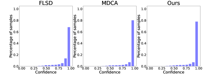
Figure 1: Histogram of confidences: Notice a rise in the number of instances falling in the last bin, ie, number of instances in the highest confidence bin in our method vs flsd [17]. While the number of instances in the highest confidence bin is nearly equal in case of mdca [6] and our method has better top-label calibration.

Refinement: Refinement also measures trust in dnns as the degree of separation between a network’s correct and incorrect predictions. Tab. 1 shows our proposed method is refined in addition to being calibrated.

Figure 2: Reliability diagrams our proposed calibration technique against the state-of-the-art methods: A ResNet50 classifier is trained on CIFAR-10 using nll, Brier-score [2], DCA [13]), Label-smoothing [18], mmce [12], flsd [17], mdca [6] and our proposed method, respectively. Reliability diagrams as a measure of calibration (When a dnns is perfectly calibrated, the accuracy for each bin would be equal to that of the confidence of that particular bin, therefore all the bars would lie on $y=x$ line. If bars are below the $y=x$ line means dnns is over-confident. If the bars are above the $y=x$ line, this means that the dnns is considered under-confident). Notice that dnns trained using nll, Brier-score, dca, ls, mmce is over-confident whereas a dnns with flsd is slightly under-confident. dnns trained using our method results in calibrated and confident predictions making our approach that uses dynamic train-time pruning appealing for practical deployment.

5.5 Ablation Study

Our proposed approach has $3$ new additions over pre-existing sota approaches. These are: (1) An auxiliary loss function, the Huber Loss that is targeted to reduce the top-label calibration; (2) A pruning step, based on predicted confidences; (3) Smoothing the confidences using an ema to enhance calibration performance. We study the effect of these individual components in this section.

Effect of varying the regularization factor ($\lambda$) on Calibration Error: We vary the effect of regularization offered by our proposed auxiliary loss function by varying $\lambda$ in Eq. 8. Plotting out the ece, ece $(S_{95})$, te, and $|S_{95}|$ and $|S_{99}|$ in Fig. 3 for a ResNet50 model trained on CIFAR-10, varying the regularization factor $\lambda$ from $\{0.1,0.5,1,5,10,25,50\}$, we gain an interesting insight into the effect of this auxiliary loss. We notice that there is a steady rise in $|S_{95}|$ and $|S_{99}|$ as $\lambda$ is increased. However, we see a minimum value of ece and ece $(S_{95})$ at $\lambda=10$. We hypothesise that an auxiliary loss between confidences and accuracies on top of calibration losses is a push-pull mechanism, the auxiliary loss tries to minimise the calibration errors by pushing the confidences up, whereas the calibration losses minimise overconfidence by pulling the confidences down. For our CIFAR-10 experiments, $\lambda=10$ proved to be the optimal balance achieving the lowest calibration errors.

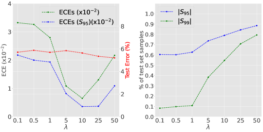
Figure 3: Effect of varying the regularization factor, $\lambda$, on training ResNet50 model on CIFAR-10 dataset. left: Plots out the ece, ece ($S_{95}$) and te vs $\lambda$. right: Studying the effect of $|S_{95}|$ and $|S_{99}|$ on varying $\lambda$. Lowest ece and ece ($S_{95}$) are achieved at $\lambda=10$. For higher values of $\lambda$($\lambda>10$), we notice an increase in $|S_{95}|$ and $|S_{99}|$, but reduction in te and calibration gets worse with $\uparrow$ in $\lambda$.

Effect of varying the pruning frequency on Calibration Error: Fig. 4 shows how varying pruning frequency affects top label calibration. As the prune interval increases we see a monotonic decrease in the te while least ece is achieved when we prune every $5$ epochs. This hints the empirical evidence that increasing pruning frequency helps in reduced calibration error.

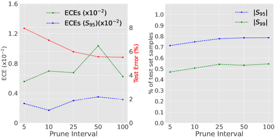
Figure 4: Effect of varying the pruning interval on training a ResNet50 on CIFAR-10 dataset. Left: Plots out the ece, ece ($S_{95}$), and te vs Pruning intervals. Pruning more frequently implies lower training time. Right: Studying the effect of $|S_{95}|$ and $|S_{99}|$ on varying the Prune Interval. Lowest ece is achieved for pruning every $5$ epochs, and best ece ($S_{95}$) is achieved for pruning every $10$ epochs.

Effect of using an ema score to track evolution of prediction confidences:

Please refer to supplementary.

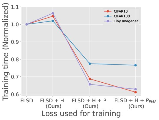
Figure 5: Comparison of training times using our proposed pruning strategy. FLSD [17], FLSD+H (Ours Eq. 8), FLSD+H+P (Ours: Eq. 8 with Pruning) and FLSD+H+$\text{P}_{\text{EMA}}$ (Ours: Eq. 8 with Pruning with exponential moving average) for a ResNet50 trained on three different datasets. Upon using our pruning strategy, we see a reduction of  20% in training time with the CIFAR100 dataset. The train time reduction while using Tiny Imagenet and CIFAR10 is  40%. Lower training times of our proposed pruning strategies make our strategy appealing for a practical viewpoint.

Reduction in training time using our proposed pruning strategy: When compared to FLSD [17], the training time of proposed approach sees a reduction of 40% in case of CIFAR10 and Tiny Imagenet Datasets, with a reduction of 20% in case of CIFAR100. Recalibration for train time calibration methods implies retraining the model on the entire train dataset. Such recalibration efforts can be unappealing given the high training times and compute required to do so. We ensure our methods provide confident and calibrated models, while reducing training time, and hence the carbon footprint significantly.

6 Conclusion

We have introduced an efficient train-time calibration method without much trade off in accuracy of dnns. We have made two contributions: first, we propose a differentiable loss term that can be used effectively in gradient descent optimisation used extensively in dnns classifiers; second, our proposed dynamic data pruning strategy not only enhances legitimate high confidence samples to enhance trust in dnns classifiers but also reduce the training time for calibration. We shed light on why pruning data facilitates high-confidence samples that aid in dnns calibration.

Supplementary Material: Calibrating Deep Neural Networks using Explicit Regularisation and Dynamic Data Pruning

Rishabh Patra^1§  Ramya Hebbalaguppe^2§  Tirtharaj Dash¹  Gautam Shroff²  Lovekesh Vig^2
1 APPCAIR, BITS Pilani, Goa Campus  ² TCS Research, New Delhi

In this supplementary document, We provide an detailed training algorithm corresponding to Procedure 2 in the main text. Further, we provide some results of calibration for the ResNet32 model in addition to the results in the main text. Our datasets, codes and the resulting models, of all our experiments (shown in the main paper and in the supplementary), will be made available publicly after acceptance.

Appendix A Datasets

We validate our proposed approach on benchmark datasets for image classification. We chose CIFAR-10/100 datasets , MendelyV2 (Medical image classification [9]), SVHN, and Tiny ImageNet. In all our experiments, we calibrate ResNet-50 [5] and measure the calibration performances using our proposed calibration technique and several other existing techniques. For all experiments, the train set is split into $2$ mutually exclusive sets: (a) training set containing $90\%$ of samples and (b) validation set: $10\%$ of the samples. The same validation set is used for post-hoc calibration.

Appendix B A detailed pruning based learning procedure

We provide additionally a detailed version of Procedure 2 from the main text. Procedure 3 details each step of our pruning based learning procedure, as used to obtain calibration DNNs with reduced training times, translating to reduced carbon footprint and easier recalibration.

Procedure 3 Our pruning-based learning procedure. The procedure takes as inputs: A dataset of $n$ instances: $D=\{(\mathbf{x}_{i},y_{i})\}_{i=1}^{n}$, An untrained neural network $\mathcal{N}$ with structure $\pi$ and parameters $\bm{\theta}$, Maximum number of training epochs: $MaxEpochs$, Batch-size: $b\leq n$, Focal loss parameter: $\gamma$, Huber Loss parameter: $\alpha$, Regularization parameter: $\lambda$, Learning rate for SGD: $\eta$, Weight decay parameter for SGD: $\beta$, EMA factor for smoothing: $\kappa$, Prune fraction: $\epsilon\in(0,100)$, A set of pruning epochs during training: $\mathbf{ep}$; and returns: a trained model. The procedure assumes a parameter update procedure BackPropWithSGD.

1:procedure TrainDNNwithDataPruning($D$,$\mathcal{N}$,$\pi$,$\bm{\theta}$,$MaxEpochs$,$b$,$\gamma$,$\alpha$,$\lambda$,$\eta$,$\beta$,$\kappa$,$\epsilon$,$\mathbf{ep}$)

2:     Let $De=\{(\mathbf{x}_{i},y_{i},0)\}_{i=1}^{n}$ where $(\mathbf{x}_{i},y_{i})\in D\}$, $i\in\{1,\dots,n\}$

3:     Number of training batches: $nb=\left\lceil\frac{n}{b}\right\rceil$

4:     Let $B_{1},\dots,B_{nb}$ be the mini-batches of data instances from $De$

5:     Initialise $\bm{\theta}$ to small random numbers

6:     for training epoch $ep$ in $\{1,\dots,MaxEpochs\}$ do

7:         for $B_{i}\in\{B_{1},\dots,B_{nb}\}$ do

8:              Mean accuracy in batch $i$: ${acc}=0$

9:              Mean confidence in batch $i$: ${conf}=0$

10:              Mean focal loss: $\mathcal{L}_{FL}=0$

11:              for each $(\mathbf{x}_{k},y_{k},e_{k})\in B_{i}$ do

12:                  $\hat{\bm{y}}=\mathcal{N}(\mathbf{x}_{k};(\pi,\bm{\theta}))$

13:                  $\hat{y}=\arg\max_{i}\hat{\bm{y}}$

14:                  $c=\max(\hat{\bm{y}})$

15:                  ${acc}={acc}+\mathbb{I}({\hat{y}=y_{k}})$

16:                  ${conf}={conf}+c$

17:                  $\mathcal{L}_{FL}=\mathcal{L}_{FL}+\text{\sc ComputeFocalLoss}(\mathrm{onehot(y_{k}),\hat{\bm{y}}},\gamma)$

18:                  $e_{k}=\kappa c+(1-\kappa)e_{k}$)

19:              end for

20:              ${acc}=acc/b$

21:              ${conf}=conf/b$

22:              $\mathcal{L}_{FL}=\mathcal{L}_{FL}/b$

23:              Calculate Huber loss: $\mathcal{L}_{H}=\text{\sc ComputeHuberLoss}(acc,conf,\alpha)$

24:              Calculate total loss: $\mathcal{L}_{total}=\mathcal{L}_{FL}+\lambda\mathcal{L}_{H}$

25:              Update parameters of $\mathcal{N}$: $\bm{\theta}=\text{\sc BackPropWithSGD}(\mathcal{L}_{total}$,$\pi$,$\bm{\theta}$,$\eta$,$\beta$)

26:         end for

27:         Update the instances in $De$ with updated ema-scores computed above

28:         if epoch $ep\in\mathbf{ep}$ then

29:              $De=\text{\sc PruneUsingEMA}(De,\epsilon)$

30:         end if

31:     end for

32:end procedure

Appendix C Additional Results with ResNet32

C.1 Experiments Parameters

The experimental parameters remain largely the same as in our ResNet50 experiments. For CIFAR10, we train the models for a total of $160$ epochs using an initial learning rate of $0.1$. The learning rate is reduced by a factor of $10$ at the $80^{th}$ and $120^{th}$ epochs. The dnns was optimized using Stochastic Gradient Descent (SGD) with momentum $0.9$ and weight decay set at $0.0005$. Further, the images belonging to the trainset are augmented using random center cropping, and horizontal flips. For CIFAR100, the models are trained for a total of $200$ epochs with a learning rate of $0.1$, reduced by a factor of $10$ at the $100^{th}$ and $150^{th}$ epochs. The batch size is set to 1024. Other parameters for training on CIFAR100 are the same ones used for CIFAR10. For Tiny-Imagenet, we follow the same training procedure used by [17]. The models are trained for $100$ epochs, with a batch size of 1024. For the Huber loss hyperparameter $\alpha$, we perform a grid search over values $\{0.001,0.005,0.01,0.05,0.1\}$. The setting $\alpha=0.005$ gave the best calibration results across all datasets, and hence we use the same value for all the experiments. For the regularization parameter $\lambda$, we perform a grid search over $\{0.1,0.5,1,5,10,25,50\}$, choosing $\lambda$ with the least ece and ece $(S_{95})$. In our ResNet32 experiments, we find that $\lambda=25$ gives the least calibration error in both the metrics for CIFAR10. For CIFAR100, $\lambda=5$ is the optimal parameter for low calibration errors. To set the pruning frequency, we again perform a grid search over $\{5,10,25,50,100\}$. We find that pruning every $25$ epochs is optimal for CIFAR10, whereas pruning every 50 epochs is optimal for CIFAR100. Needless to say, we identify our optimal parameters as those which provide the least calibration error.

Effect of using an ema score to track evolution of prediction confidences:

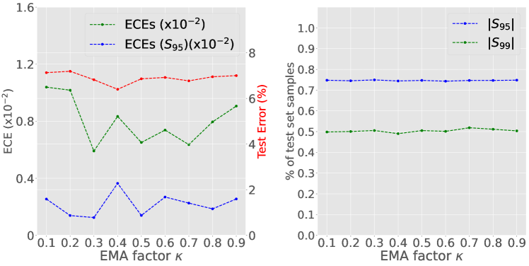
Figure 6: Effect of varying the EMA factor ($\kappa$) on training a ResNet50 on CIFAR-10 dataset. Left: Plots out the ece, ece ($S_{95}$), and te vs. ema factor, $\kappa$. Right: Study of the effect of $|S_{95}|$ and $|S_{99}|$ on varying $\kappa$. The best ece and ece ($|S_{95}|$) are achieved at $\kappa=0.3$. Varying $\kappa$ has no noticeable effect of $|S_{95}|$ and $|S_{99}|$

We show how the te, ece, ece ($S_{95}$), $|S_{95}|$ and $S_{99}$ vary with increasing the ema factor $\kappa$. There isn’t any noticeable trend of metrics across varying $\kappa$. However, using an ema score to track confidences across epochs, and subsequently using this ema score to prune training instances is a practically appealing method since it produces near perfect calibration of the high confidence instances.

C.2 Experimental Results

		BS [2]			DCA [13]			LS [24]			MMCE [12]			FLSD [17]			FL + MDCA [6]			Ours (FLSD+H+$\text{P}_{\text{EMA}}$)
Dataset	Model	ECE	TE	AUROC	ECE	TE	AUROC	ECE	TE	AUROC	ECE	TE	AUROC	ECE	TE	AUROC	ECE	TE	AUROC	ECE	TE	AUROC
CIFAR10	ResNet32	2.83	7.67	90.35	3.58	17.13	87.39	3.06	7.71	85.25	4.16	7.36	90.81	5.27	7.82	91.24	0.93	7.18	91.62	1.10	8.33	91.42
CIFAR100	ResNet32	7.87	36.78	85.67	7.82	42.91	82.46	7.44	34.66	83.52	15.09	33.33	84.48	3.28	35.7	82.91	3.06	35.47	83.39	3.18	35.41	82.36

Table 3: Calibration measure ece (%) score), Test Error (te) (%) and AUROC (refinement) in comparison with various competing methods. We use $M=10$ bins for ece calculation. We outperform most of the baselines across various popular benchmark datasets, and architectures in terms of calibration, while maintaining a similar accuracy and a similiar refinement (AUROC.)

		BS [2]		DCA [13]		LS [7]		MMCE [12]		FLSD [17]		FL + MDCA [6]		Ours (FLSD+H+$\text{P}_{\text{EMA}}$)
Dataset	Model	ECE ($S_{95}$)	$|S_{95}|$	ECE ($S_{95}$)	$|S_{95}|$	ECE ($S_{95}$)	$|S_{95}|$	ECE ($S_{95}$)	$|S_{95}|$	ECE ($S_{95}$)	$|S_{95}|$	ECE ($S_{95}$)	$|S_{95}|$	ECE ($S_{95}$)	$|S_{95}|$
CIFAR10	ResNet32	1.49	82.44	1.29	54.74	1.55	74.46	2.54	87.80	2.36	40.52	1.56	57.63	0.002	72.36
CIFAR100	ResNet32	3.47	33.34	2.26	20.28	3.31	28.40	7.84	46.63	0.54	16.47	0.11	17.07	0.008	17.37

Table 4: Top-label calibration measure ECE ($S_{95}$) (% score) and $|S_{95}|$ (percentage of total number of test samples with predictive confidences $\geq 0.95$) in comparison with various competing methods. We use $M=10$ bins for ECE ($S_{95}$) calculations. We outperform all the baselines across various popular benchmark datasets, and architectures in terms of calibration. While we do not outperform all calibration methods in terms of $|S_{95}|$,it is to be noted that we obtain a higher $|S_{95}|$ than (flsd, mdca).

Tab. 3 shows the te, ece and AUROC for refinement of the ResNet32 models trained on CIFAR10. We notice that mdca outperforms our proposed approach in terms of ece. However, it is to be noted that our proposed approach is better calibrated than all the other sota approaches. Tab. 4 shows the ece ($S_{95}$) and $|S_{95}|$ for our ResNet32 experiments. Here, we obtain the least ece ($S_{95}$) against all other sota approaches, which is in alignment with our claims of our approach being appealing for practical scenarios. Further, we obtain better $|S_{95}|$ than other Focal loss based methods (ie. mdca, flsd).

References

- [1] Ondrej Bohdal, Yongxin Yang, and Timothy Hospedales. Meta-calibration: Meta-learning of model calibration using differentiable expected calibration error. In ICML Uncertainity in Deep Learning Workshop, 2021.
- [2] Glenn W Brier et al. Verification of forecasts expressed in terms of probability. Monthly weather review, 78(1):1–3, 1950.
- [3] Arthur Gretton. Introduction to rkhs, and some simple kernel algorithms. Adv. Top. Mach. Learn. Lecture Conducted from University College London, 16:5–3, 2013.
- [4] Chuan Guo, Geoff Pleiss, Yu Sun, and Kilian Q Weinberger. On calibration of modern neural networks. In ICML, pages 1321–1330. PMLR, 2017.
- [5] Kaiming He, Xiangyu Zhang, Shaoqing Ren, and Jian Sun. Deep residual learning for image recognition, 2015.
- [6] Ramya Hebbalaguppe, Jatin Prakash, Neelabh Madan, and Chetan Arora. A stitch in time saves nine: A train-time regularizing loss for improved neural network calibration. In IEEE/CVF CVPR, June 2022.
- [7] Geoffrey Hinton, Oriol Vinyals, and Jeff Dean. Distilling the knowledge in a neural network. arXiv preprint arXiv:1503.02531, 2015.
- [8] Peter J Huber. Robust estimation of a location parameter. In Breakthroughs in statistics, pages 492–518. Springer, 1992.
- [9] Daniel Kermany, Kang Zhang, Michael Goldbaum, et al. Labeled optical coherence tomography (oct) and chest x-ray images for classification. Mendeley data, 2(2), 2018.
- [10] Meelis Kull, Miquel Perello-Nieto, Markus Kängsepp, Hao Song, Peter Flach, et al. Beyond temperature scaling: Obtaining well-calibrated multiclass probabilities with dirichlet calibration. arXiv preprint arXiv:1910.12656, 2019.
- [11] Meelis Kull, Telmo Silva Filho, and Peter Flach. Beta calibration: a well-founded and easily implemented improvement on logistic calibration for binary classifiers. In Artificial Intelligence and Statistics, pages 623–631. PMLR, 2017.
- [12] Aviral Kumar, Sunita Sarawagi, and Ujjwal Jain. Trainable calibration measures for neural networks from kernel mean embeddings. In ICML, pages 2805–2814, 2018.
- [13] Gongbo Liang, Yu Zhang, Xiaoqin Wang, and Nathan Jacobs. Improved trainable calibration method for neural networks on medical imaging classification. CoRR, abs/2009.04057, 2020.
- [14] Tsung-Yi Lin, Priya Goyal, Ross Girshick, Kaiming He, and Piotr Dollár. Focal loss for dense object detection. In Proceedings of the IEEE ICCV, pages 2980–2988, 2017.
- [15] Kushagra Mahajan, Monika Sharma, Lovekesh Vig, Rishab Khincha, Soundarya Krishnan, Adithya Niranjan, Tirtharaj Dash, Ashwin Srinivasan, and Gautam Shroff. CovidDiagnosis: Deep Diagnosis of COVID-19 Patients Using Chest X-Rays. In International Workshop on Thoracic Image Analysis, pages 61–73. Springer, 2020.
- [16] Jishnu Mukhoti, Viveka Kulharia, Amartya Sanyal, Stuart Golodetz, Philip HS Torr, and Puneet K Dokania. Calibrating deep neural networks using focal loss. arXiv preprint arXiv:2002.09437, 2020.
- [17] Jishnu Mukhoti, Viveka Kulharia, Amartya Sanyal, Stuart Golodetz, Philip H. S. Torr, and Puneet K. Dokania. Calibrating deep neural networks using focal loss, 2020.
- [18] Rafael Müller, Simon Kornblith, and Geoffrey Hinton. When does label smoothing help? arXiv preprint arXiv:1906.02629, 2019.
- [19] Yaniv Ovadia, Emily Fertig, Jie Ren, Zachary Nado, David Sculley, Sebastian Nowozin, Joshua V Dillon, Balaji Lakshminarayanan, and Jasper Snoek. Can you trust your model’s uncertainty? evaluating predictive uncertainty under dataset shift. arXiv preprint arXiv:1906.02530, 2019.
- [20] Mansheej Paul, Surya Ganguli, and Gintare Karolina Dziugaite. Deep learning on a data diet: Finding important examples early in training. Advances in Neural Information Processing Systems, 34, 2021.
- [21] Gabriel Pereyra, George Tucker, Jan Chorowski, Łukasz Kaiser, and Geoffrey Hinton. Regularizing neural networks by penalizing confident output distributions. arXiv preprint arXiv:1701.06548, 2017.
- [22] John Platt et al. Probabilistic outputs for support vector machines and comparisons to regularized likelihood methods. Advances in large margin classifiers, 10(3):61–74, 1999.
- [23] Aditya Singh, Alessandro Bay, Biswa Sengupta, and Andrea Mirabile. On deep neural network calibration by regularization and its impact on refinement. arXiv preprint arXiv:2106.09385, 2021.
- [24] Christian Szegedy, Vincent Vanhoucke, Sergey Ioffe, Jonathon Shlens, and Zbigniew Wojna. Rethinking the inception architecture for computer vision, 2015.
- [25] Mariya Toneva, Alessandro Sordoni, Remi Tachet des Combes, Adam Trischler, Yoshua Bengio, and Geoffrey J. Gordon. An empirical study of example forgetting during deep neural network learning. In ICLR, 2019.