Conditioned Generative Transformers for Histopathology Image Synthetic Augmentation

Abstract

Deep learning networks have demonstrated state-of-the-art performance on medical image analysis tasks. However, the majority of the works rely heavily on abundantly labeled data, which necessitates extensive involvement of domain experts. Vision transformer (ViT) based generative adversarial networks (GANs) recently demonstrated superior potential in general image synthesis, yet are less explored for histopathology images. In this paper, we address these challenges by proposing a pure ViT-based conditional GAN model for histopathology image synthetic augmentation. To alleviate training instability and improve generation robustness, we first introduce a conditioned class projection method to facilitate class separation. We then implement a multi-loss weighing function to dynamically balance the losses between classification tasks. We further propose a selective augmentation mechanism to actively choose the appropriate generated images and bring additional performance improvements. Extensive experiments on the histopathology datasets show that leveraging our synthetic augmentation framework results in significant and consistent improvements in classification performance.

1 Introduction

Vision transformer (ViT) [25] models have started to outperform convolutional neural networks (CNNs) in various image tasks [5, 24, 8, 3]. Recently, a few pioneering studies have published convolution-free ViT-based GANs and demonstrated good performance on image generation tasks [15, 17]. Different from the local receptive field in CNN, ViTs have exhibited promising superiority in modeling non-local contextual dependencies [17]. One known attribute of histopathology images is that they commonly comprise various non-local or long-range information [27]. As a result, at the infancy stage, these convolution-free ViT-based GAN models are considered to have great potential for histopathology image analysis tasks.

Deep learning has benefited from abundantly labeled data and achieves good performance on the histopathological image analysis tasks. However, most of the works come at the expense of acquiring much labeled data and require the extensive participation of domain experts [20]. The whole process is labor-intensive and time-consuming, which is impractical for rare diseases, early clinical studies, or new imaging modalities [19]. A few works have been proposed to mitigate the aforementioned issues by employing GANs to generate synthetic images for data augmentation and achieved satisfactory results [20, 9, 7]. Nonetheless, these works split the image generation and data augmentation into two stages, which results in different models for each stage and requires more effort to train.

We address the aforementioned challenges by introducing a framework that adopts a convolution-free ViT-based GAN model for histopathology image synthetic augmentation. The framework merges models from two stages into one, which not only conditionally generates synthesized images but also performs classification prediction. This is a challenging task, as GANs are known to be prone to notorious training instability [15], combining multiple losses would lead to extra unstable performance. As a result, we first propose a conditioned class projection to assist in the separation of the conditional information during training. Inspired by the success of multi-task learning works [16, 22], we then introduce a novel multi-loss weighing function to balance the losses when training our conditional GAN model. To improve synthetic augmentation performance even further, we introduce a selective augmentation mechanism that actively selects appropriate images for augmentation.

To summarize, the major contributions of this paper can be listed as follows:

• To the best of our knowledge, this work is among the first to explore conditional convolution-free ViT-based GANs on histopathology images, which is of great practical value and less studied by previous literature.

• We introduce a novel conditioned class projection method to facilitate class separation during training.

• We address the problem that two-stage image synthetic augmentation in previous works results in low efficiency. To this end, we propose a novel all-in-one framework by using a multi-loss weighing function. This helps stabilize training and improves performance on each task.

• We propose a selective augmentation mechanism to further increase the synthetic augmentation performance.

• Extensive experiments are conducted on lymph node histopathology datasets. Compared with baseline models, experimental results show that our proposed method significantly improves the augmented classification performance.

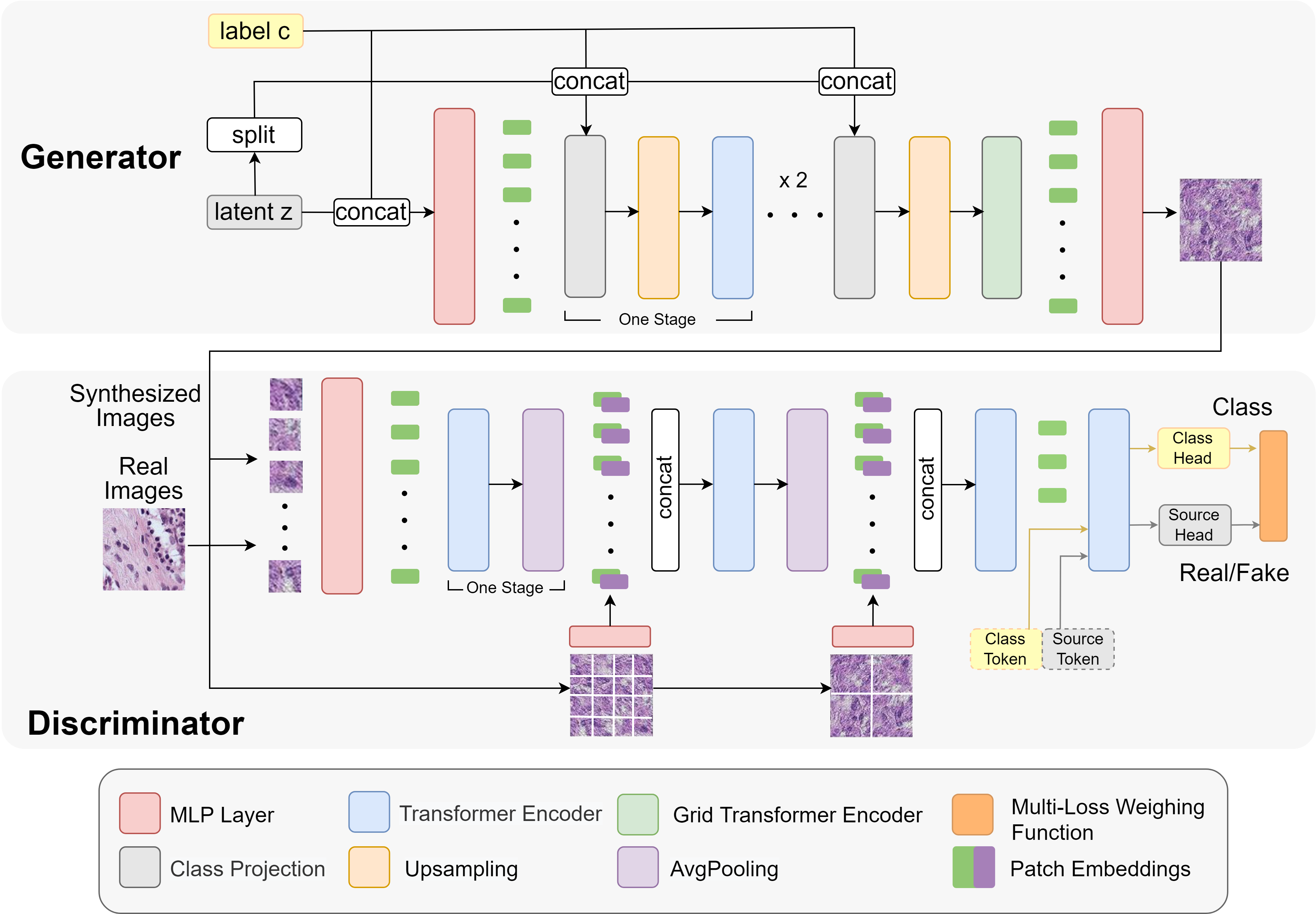
Figure 1: Overview of our proposed network. In the generator, the latent vector $z$ is split into multiple chunks and concatenated with conditional label $c$ as the inputs to class projection layer. One generator block includes a class projection layer, an upsampling layer, and a transformer encoder. One discriminator block includes a transformer encoder and an average pooling layer. A multi-scale pyramid technique is employed to learn global and local information. The output of discriminator is the adaptive weighing function of the class and source losses.

2 Method

The overall framework of our proposed transformer-based GAN is shown in Fig. 1. Unlike other transformer-integrated GANs [29, 6] for medical image synthesis, our model is constructed entirely of transformer components and is CNN-free. We adopt a conditional training strategy by introducing multiple class projection modules in the generator, and an additional class token in the discriminator to perform the classification task. The outputs of class and source heads are adaptively combined through our proposed multi-loss weighing function.

2.1 Transformer-based GAN

Our proposed model is a pure transformer-based GAN following the design of TransGAN [15]. The primary component is the ViT encoder [8], which comprises multi-head self-attention modules, including query, key, and value representations to conduct a self-attention scaled dot-product computation. Next, the output goes through a feed-forward multi-layer perceptron (MLP) layer with GELU non-linearity [12]. Both parts employ residual connection and layer normalization techniques.

The generator of the proposed GAN comprises four-stage blocks that gradually learn and upsample the latent vector $z$. Initially, the latent vector noise $z$ is concatenated with the one-hot label $c$ and passed through a linear projection layer to generate embedding tokens. Each block consists of a class projection layer, an upsampling module, and four ViT encoders. By stages, the generator progressively increases the feature map resolution until it reaches the predefined dimension $H\times W$. In the first stage, the embedded feature map is upsampled from $X_{i}\in\mathbb{R}^{H_{i}\times W_{i}\times C}$ to $X_{i}^{\prime}\in\mathbb{R}^{2H_{i}\times 2W_{i}\times C}$ by cubic interpolation without dimension reduction, which guarantees the early feature learning. The next three stages adopt a pixel-shuffle module [23] that upsamples the feature map while decreasing the channels to a quarter. The feature map then converts from $X_{i}\in\mathbb{R}^{H_{i}\times W_{i}\times C}$ to $X_{i}^{\prime}\in\mathbb{R}^{2H_{i}\times 2W_{i}\times\frac{C}{4}}$. This reduces memory requirements and makes the network more efficient. As the self-attention layer is prone to learn global correspondence while neglecting local information [15], for the third and fourth stages, we use grid transformer encoders to constrain the model to learn local details of the image. This is achieved by reshaping the feature map size to the predefined dimension that goes through the ViT encoders. In our model, we set the predefined window size to $32\times 32$ for the third stage and $16\times 16$ for the fourth stage.

The discriminator consists of four stages. Each of the first three includes a ViT encoder and an average pooling layer. Between the stages, a multi-scale technique is employed by combining the outputs from the last block with the varying sizes of patches from the same input image. After an MLP layer, the patch information is encoded in a sequence of embeddings for concatenation. This is to let the model learn both semantic structure and texture details. To enable conditional learning, at the end of the third block, a class token and a source token are appended at the beginning of the 1D sequence and go through the fourth stage with two ViT encoders. The tokens are taken by the classification head and the source head to output the class and real/fake predictions.

2.2 Conditioned Class Projection

To further improve the conditional image generation, we first adopt a direct skip connection (skip-z) [4] method that splits noise vector $z$ into multiple chunks and adds connections to the four stages in our proposed generator. The intuition behind this design is to enable the generator to use the latent space that directly affects features generated at different resolutions. More specifically, we split $z$ into one chunk per stage, and concatenate each chunk to the class vector $c$. The combination is then passed into the class projection layer.

Next, we implement the class projection onto the token embeddings. We call this approach conditional layer normalization. In contrast to the class-conditional [4] method that uses batch normalization, we find that employing layer normalization [2] for ViT-based conditional GAN obtains superior performance. The approach transforms a layer’s activations $a$ into a normalized activation $\bar{a}$ specific to class condition, which is shown as:

$$\bar{a}=\frac{a-\hat{\mu}}{\sqrt{\hat{\sigma}+\epsilon}}*\gamma+\beta.$$ (1)

Where $\hat{\mu}$ and $\hat{\sigma}$ stands for mean and variance of the input, $\epsilon$ is a small value added to the denominator for numerical stability. Specifically, we inject class-conditional information by parameterizing $\gamma$ and $\beta$ as linear transformations of the class embedding, $c$, where $\gamma:=W_{\gamma}^{\top}[c,z]$ and $\beta:=W_{\beta}^{\top}[c,z]$, $[c,z]$ denotes the concatenation of $c$ and $z$ in skip connections.

2.3 Selective Data Augmentation

We further improve synthetic augmentation performance by employing a selective data augmentation mechanism. To ensure a high fidelity image generation, we first adopt a truncation method [18] which resamples $z$ from a truncated normal distribution by a truncation value $\tau$. After generating the images conditionally, we use our trained classification head of the same model to assist in selecting qualified augmentation images. Only the image prediction confidence value greater than threshold $\lambda$ will be used. We find $\tau=0.7$ and $\lambda=0.6$ achieves best performance in our experiments.

2.4 Multi-Loss Weighing Function

The learning strategy of our network follows AC-GAN [21] by incorporating an auxiliary class head in the discriminator. However, the auxiliary classifier in [21] primarily serves as a control for diversified image generation yet obtains downgraded classification performance. In our work, we aim to address this problem by incorporating a multi-loss weighing function that adapts WGAN-GP loss [1] and classification cross-entropy loss, so that the generation and classification both achieve satisfying results.

We apply Wasserstein loss with gradient penalty [1, 10] to our GAN. The objective is given by:

$$\mathcal{L}_{S}=\min_{G}\max_{D\in\mathcal{D}}\underset{x\sim\mathbb{P}_{r}}{\mathbb{E}}[D(x)]-\underset{z\sim\mathbb{P}_{z}}{\mathbb{E}}[D(G(c,z))]+\lambda\underset{\hat{\boldsymbol{x}}\sim\mathbb{P}_{\hat{x}}}{\mathbb{E}}\left[\left(\left\|\nabla_{\hat{\boldsymbol{x}}}D(\hat{\boldsymbol{x}})\right\|_{2}-1\right)^{2}\right],$$ (2)

where $D$ is the critic head of discriminator that describes a group of 1-Lipschitz functions and $G$ is the generator. $\mathbb{P}_{r}$, $\mathbb{P}_{z}$, and $\mathbb{P}_{\hat{x}}$ donate the distribution of real data $x$, the normal distribution of a random $z$, and the distribution of pairs of points from $\mathbb{P}_{r}$ and $\mathbb{P}_{z}$. Every generated sample has a corresponding class label $c\sim\mathbb{P}_{c}$ besides $z$. $G$ uses conditioned noise to generate images $X_{\text{fake }}=G(c,z)$. Note that the critic head does not involve conditioned information.

To enable conditional learning, we employ an auxiliary classification head $P(C\mid X)$ on discriminator, the log-likelihood objective function is given by:

$$\mathcal{L}_{C}=\mathbb{E}\left[\log P\left(C=c\mid X_{\text{real }}\right)\right]+\mathbb{E}\left[\log P\left(C=c\mid X_{\text{fake }}\right)\right],$$ (3)

both $D$ and $G$ are trained to maximize $\mathcal{L}_{C}$. We find that simply combining $\mathcal{L}_{C}$ and $\mathcal{L}_{S}$ is prone to result in training failure as WGAN loss value is relatively large at most times, which results in cross-entropy loss overwhelmed during training. In addition, the model tends to be good at one classification task on discriminator which results in an imbalance problem. To this end, we employ the concept from the multi-task learning realm [16] to weigh classification losses. Kendall et al. [16] proposed a strategy to balance multi-task losses by considering the uncertainty of each task, which is shown as:

$$\mathcal{L}_{\text{joint}}\left(\gamma_{1},\gamma_{2}\right)=\frac{1}{2\gamma_{1}^{2}}\mathcal{L}_{1}+\frac{1}{2\gamma_{2}^{2}}\mathcal{L}_{2}+\log\gamma_{1}+\log\gamma_{2},$$ (4)

where $\mathcal{L}_{1,2}$ represent the losses of classification tasks, $\gamma_{1,2}$ are trainable parameters representing the positive scalar of each task.

During training, we observe that the range of scalar values affects model performance (details in Section 3) as they can only be positive in $log$ form, we therefore propose a modified multi-loss weighting strategy which allows them to be in the range $[-\infty,+\infty]$. Specifically, we use $\exp\left(-\sigma\right)$ as the trainable scaling parameter to replace $\frac{1}{2\gamma_{1}^{2}}$, which allows $\sigma$ to be an unlimited regularization value. Let $f^{\theta}(x)$ be the output of the critic head with weights $\theta$, our adapted classification likelihood of the model output through softmax function can be written as:

$$p\left(\mathbf{y}\mid\mathbf{f}^{\mathbf{\theta}}(\mathbf{x}),\sigma\right)=\operatorname{Softmax}\left(\exp(-\sigma)\mathbf{f}^{\mathbf{\theta}}(\mathbf{x})\right)$$ (5)

with an unlimited range trainable scalar $\sigma$. The scaling process can be regarded as a Maxwell–Boltzmann distribution, where $\exp(-\sigma)$ is commonly referred to as temperature of the input. The learnable parameter’s magnitude determines how “flat” the discrete distribution is. The output is then related to uncertainty by using the log likelihood, which can then be written as:

$$-\operatorname{log}p\left(\mathbf{y}=c\mid\mathbf{f}^{\mathbf{\theta}}(\mathbf{x}),\sigma\right) =-\operatorname{logSoftmax}\left(\exp(-\sigma)\mathbf{f}_{c}^{\theta}\left(x\right)\right)$$ (6)

$$=-\operatorname{log}\frac{\exp[\exp(-\sigma)\mathbf{f}^{\theta}_{c}(x)]}{\sum_{c^{\prime}}\exp[\exp(-\sigma)\mathbf{f}^{\theta}_{c^{\prime}}(x)]}$$

$$=-\exp(-\sigma)\mathbf{f}^{\theta}_{c}\left(x\right)+\operatorname{log}\sum_{c^{\prime}}\exp[\exp(-\sigma)\mathbf{f}_{c^{\prime}}^{\theta}\left(x\right)]$$

$$=-\exp(-\sigma)\operatorname{log}[\frac{\exp({\mathbf{f}^{\theta}_{c}(x))}}{\sum_{c^{\prime}}\exp({\mathbf{f}^{\theta}_{c^{\prime}}(x))}}]$$

$$\,\quad+\operatorname{log}\frac{\sum_{c^{\prime}}\exp[\exp(-\sigma)\mathbf{f}^{\theta}_{c^{\prime}}(x)]}{\left(\sum_{c^{\prime}}\exp({\mathbf{f}^{\theta}_{c^{\prime}}(x))}\right)^{\exp(-\sigma)}}$$

$$\approx\exp(-\sigma)\mathcal{L}+\sigma,$$

where $-\exp(-\sigma)\operatorname{log}[\frac{\exp({\mathbf{f}^{\theta}_{c}(x))}}{\sum_{c^{\prime}}\exp({\mathbf{f}^{\theta}_{c^{\prime}}(x))}}]=-\exp(-\sigma)\operatorname{logSoftmax}\left(\mathbf{y},\mathbf{f}^{\theta}(x)\right)$ is our scaled loss function. We write $\mathcal{L}=-\operatorname{logSoftmax}\left(\mathbf{y},\mathbf{f}^{\theta}(x)\right)$ for the cross entropy loss (not scaled). In the last transition, an explicit simplifying assumption is introduced:

$$\exp(-\sigma)\sum_{c^{\prime}}\exp\left[\exp(-\sigma)f_{c^{\prime}}^{\mathrm{\theta}}(\mathbf{x})\right]\approx\left(\sum_{c^{\prime}}\exp\left(f_{c^{\prime}}^{\mathrm{\theta}}(\mathbf{x})\right)\right)^{\exp(-\sigma)},$$ (7)

When $\sigma\longrightarrow 0$, Eq 7 becomes equality. This helps simplify the optimisation objective and empirically demonstrates promising results.

Given multiple classification outputs from the critic head, we often define the likelihood to factorise over the outputs. Our multi-task likelihood is shown as follows:

$$p\left(\mathbf{y_{1}},\mathbf{y_{2}},\mathbf{y_{3}}\mid\mathbf{f}^{\mathbf{\theta}}(\mathbf{x})\right)=p\left(\mathbf{y_{1}},\mid\mathbf{f}^{\mathbf{\theta}}(\mathbf{x})\right)p\left(\mathbf{y_{2}},\mid\mathbf{f}^{\mathbf{\theta}}(\mathbf{x})\right)p\left(\mathbf{y_{3}},\mid\mathbf{f}^{\mathbf{\theta}}(\mathbf{x})\right),$$ (8)

where $\mathbf{y}_{1,2,3}$ represent classification predictions of fake data from generator, and real and fake data from discriminator. Next, the joint loss of weighted log likelihood of multi classification tasks is given as:

$$\mathcal{L}_{weighting} =-\operatorname{log}p\left(\mathbf{y_{1}},\mathbf{y_{2}},\mathbf{y_{3}}=c_{1},c_{2},c_{3}\mid\mathbf{f}^{\mathbf{\theta}}(\mathbf{x}),\sigma_{1},\sigma_{2},\sigma_{3}\right)$$ (9)

$$=-[\operatorname{log}p\left(\mathbf{y_{1}}=c_{1}\mid\mathbf{f}^{\mathbf{\theta}}(\mathbf{x}),\sigma_{1}\right)+\operatorname{log}p\left(\mathbf{y_{2}}=c_{2}\mid\mathbf{f}^{\mathbf{\theta}}(\mathbf{x}),\sigma_{2}\right)$$

$$\,\quad+\operatorname{log}p\left(\mathbf{y_{3}}=c_{3}\mid\mathbf{f}^{\mathbf{\theta}}(\mathbf{x}),\sigma_{3}\right)]$$

$$=\exp(-\sigma_{1})\mathcal{L}_{1}(\mathbf{\theta})+\exp(-\sigma_{2})\mathcal{L}_{2}(\mathbf{\theta})+\exp(-\sigma_{3})\mathcal{L}_{3}(\mathbf{\theta})+\sigma_{1}+\sigma_{2}+\sigma_{3}$$

The final weighted objective can be regarded as learning each task weights of each output losses. Larger temperature value $\sigma$ gives less contribution of loss function, while smaller $\sigma$ increases its weight. The function is regulated by the last three terms when $\sigma$ is too small.

3 Experiments

3.1 Datasets

Our experiments are conducted on the public PatchCamelyon (PCam) benchmark dataset [26]. The PCam dataset consists of 327,680 color images derived and digitized using a 40x objective (resultant pixel resolution of 0.243 microns) from lymph node sections. Each patch is of 96 $\times$ 96 resolution and split into two classes based on whether a metastatic tissue is present in the center region. The dataset is divided into 75%:12.5%:12.5% for training, validation, and testing utilizing a hard-negative mining regime. To mimic the situation where limited training data is available, we randomly choose 10% of the images from training data (32768). The whole test set is used to evaluate the augmentation performance.

3.2 Implementation Details

Our network is built based on a pure transformer architecture [15], details are shown in supplementary materials. In the experiment, we use two Tesla V100 GPUs of 16G of RAM each. An Adam optimizer with $\beta_{1}=0$, $\beta_{2}=0.99$, and the learning rate $1e-4$ is adopted to tune both generator and discriminator. The batch size is 12 for both generator and discriminator. During training, we run 500 epochs for all experiments and choose the best epoch based on the Frechet Inception Distance (FID) [13] score between generated images and validation data. We implement DiffAug. [30] as our augmentation strategy during the training process. The augmentation policy adopted in our experiment includes random color transforms, translation, cutout, scaling, and rotation.

Table 1: Evaluation of different models for our data synthesis augmentation method. Aug: augmentation. CP: conditional projection. SA: selective augmentation.

	Accuracy	AUC	Sensitivity	Specificity
Resnet34 [11]	0.881 $\pm$ 0.079	0.945 $\pm$ 0.022	0.846 $\pm$ 0.086	0.916 $\pm$ 0.020
Resnet34+Aug(MedViTGAN)	0.912 $\pm$ 0.154	0.968 $\pm$ 0.089	0.882 $\pm$ 0.092	0.942 $\pm$ 0.071
Resnet34+Aug(CP)	0.900 $\pm$ 0.060	0.949 $\pm$ 0.064	0.868 $\pm$ 0.031	0.929 $\pm$ 0.293
Resnet34+Aug(SA)	0.908 $\pm$ 0.083	0.958 $\pm$ 0.082	0.866 $\pm$ 0.122	0.929 $\pm$ 0.029
Resnet34+Aug(CP+SA)	0.916 $\pm$ 0.144	0.954 $\pm$ 0.042	0.891 $\pm$ 0.100	0.951 $\pm$ 0.109
Resnet50_CBAM [28]	0.899 $\pm$ 0.131	0.955 $\pm$ 0.045	0.863 $\pm$ 0.096	0.935 $\pm$ 0.040
Resnet50_CBAM+Aug(MedViTGAN)	0.918 $\pm$ 0.230	0.930 $\pm$ 0.021	0.821 $\pm$ 0.123	0.917 $\pm$ 0.066
Resnet50_CBAM+Aug(CP)	0.920 $\pm$ 0.180	0.959 $\pm$ 0.055	0.880 $\pm$ 0.040	0.937 $\pm$ 0.088
Resnet50_CBAM+Aug(SA)	0.916 $\pm$ 0.039	0.959 $\pm$ 0.062	0.876 $\pm$ 0.112	0.941 $\pm$ 0.137
Resnet50_CBAM+Aug(CP+SA)	0.922 $\pm$ 0.077	0.962 $\pm$ 0.046	0.879 $\pm$ 0.047	0.945 $\pm$ 0.110
Densenet169 [14]	0.894 $\pm$ 0.059	0.955 $\pm$ 0.036	0.881 $\pm$ 0.094	0.908 $\pm$ 0.032
Densenet169+Aug(MedViTGAN)	0.927 $\pm$ 0.025	0.974 $\pm$ 0.040	0.867 $\pm$ 0.049	0.966 $\pm$ 0.052
Densenet169+Aug(CP)	0.900 $\pm$ 0.177	0.946 $\pm$ 0.074	0.879 $\pm$ 0.099	0.904 $\pm$ 0.107
Densenet169+Aug(SA)	0.917 $\pm$ 0.021	0.975 $\pm$ 0.066	0.877 $\pm$ 0.131	0.956 $\pm$ 0.099
Densenet169+Aug(CP+SA)	0.928 $\pm$ 0.076	0.960 $\pm$ 0.049	0.898 $\pm$ 0.125	0.967 $\pm$ 0.092
MedViTGAN Cls Head	0.939 $\pm$ 0.059	0.980 $\pm$ 0.073	0.906 $\pm$ 0.079	0.974 $\pm$ 0.054
HViTGAN Cls Head (ours)	0.916 $\pm$ 0.070	0.971 $\pm$ 0.098	0.900 $\pm$ 0.033	0.923 $\pm$ 0.081
HViTGAN Cls Head (ours)+Aug(CP)	0.931 $\pm$ 0.029	0.966 $\pm$ 0.101	0.897 $\pm$ 0.277	0.957 $\pm$ 0.123
HViTGAN Cls Head (ours)+Aug(SA)	0.929 $\pm$ 0.110	0.977 $\pm$ 0.093	0.889 $\pm$ 0.042	0.961 $\pm$ 0.069
HViTGAN Cls Head (ours)+Aug(CP+SA)	0.945 $\pm$ 0.054	0.981 $\pm$ 0.045	0.910 $\pm$ 0.063	0.977 $\pm$ 0.102

3.3 Discussion and Comparisons

We report quantitative evaluation scores between all selected baseline models and our synthetic augmentation method. They are the accuracy, the area under the ROC curve (AUC), sensitivity, and specificity for a comprehensive comparison. All models were executed for five repetitions with random initialization for a fair comparison. The mean and standard deviation were reported. As is shown in Table 1, we conducted our experiments on representative baseline models with same settings for comprehensive study, including Resnet34 [11], Resnet50 CBAM [28], Densenet169 [14], and our model’s classification head for both baseline and augmentation training. The results consistently showed that with the augmentation of our synthesized images, the models obtained superior performance compared to baselines. We also analyzed how different loss functions affect the generated images. As shown in Fig. 3, we compared seven scenarios for loss functions. Experiments showed that WGAN-GP loss was significantly scaled-down after applying weight to it which resulted in inferior performance. Hence, we omitted the weight applied to WGAN-GP loss and formed our multi-loss weighing function. Our method demonstrated the best image separation performance. More details can be found in the supplementary materials. As demonstrated in Fig. 2, the synthetic images have comparable quality in terms of both fidelity and diversity. We therefore believe that our proposed model is capable of handling other histopathology image-associated tasks with insufficient training data.

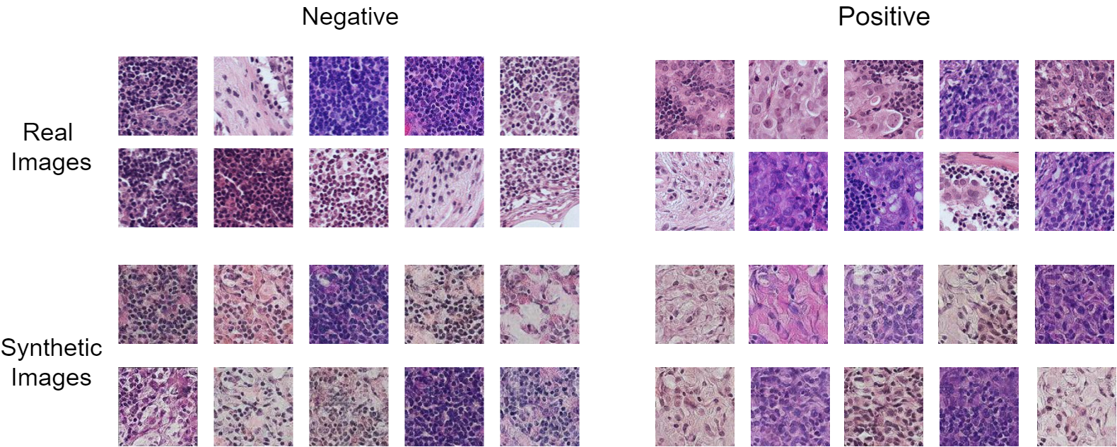
Figure 2: Selected real and synthetic images generated by the proposed model trained on 10% of PCam dataset. SA: selective augmentation. CP: conditional projection

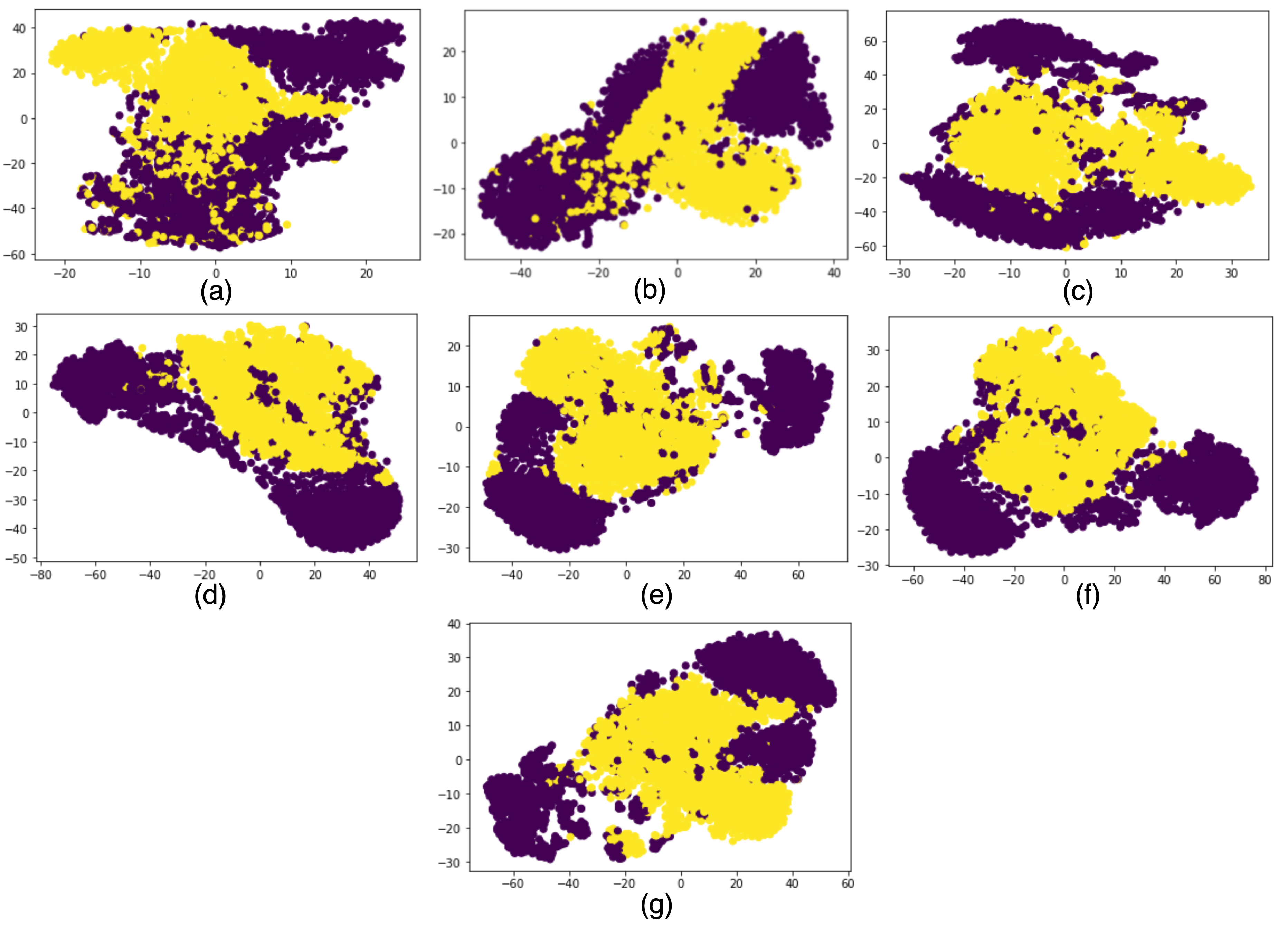
Figure 3: T-SNE graphs for generated images with different loss scenarios. (a) No weighting function applied to individual loss. (b) Weighting function applied to all losses. (c) Kendall et al. [16] weighting function. (d) Our weighting function. (e) Our weighting function with CP. (f) Our weighting function with SA. (g) Our weighting function with CP+SA. CP: conditional projection. SA: selective augmentation.

4 Conclusion

In this paper, we introduce a pure ViT-based conditional GAN framework for histopathology image synthetic augmentation that incorporates several novel techniques. To enable conditional learning, we employ an auxiliary discriminator head for classification. We further improve the training by proposing several novel techniques including conditioned class projection, multi-loss weighing function, and selective augmentation mechanism. Experimental results demonstrate that our approach makes a significant improvement over baseline methods. In future work, we plan to generalize our model to natural image tasks. Additionally, larger networks will be examined to generate high-resolution images.

References

- [1] Arjovsky, M., Chintala, S., Bottou, L.: Wasserstein generative adversarial networks. In: International conference on machine learning. pp. 214–223. PMLR (2017)
- [2] Ba, J.L., Kiros, J.R., Hinton, G.E.: Layer normalization. arXiv preprint arXiv:1607.06450 (2016)
- [3] Bertasius, G., Wang, H., Torresani, L.: Is space-time attention all you need for video understanding? arXiv preprint arXiv:2102.05095 (2021)
- [4] Brock, A., Donahue, J., Simonyan, K.: Large scale gan training for high fidelity natural image synthesis. arXiv preprint arXiv:1809.11096 (2018)
- [5] Chen, M., Radford, A., Child, R., Wu, J., Jun, H., Luan, D., Sutskever, I.: Generative pretraining from pixels. In: International Conference on Machine Learning. pp. 1691–1703. PMLR (2020)
- [6] Dalmaz, O., Yurt, M., Çukur, T.: Resvit: Residual vision transformers for multi-modal medical image synthesis. arXiv preprint arXiv:2106.16031 (2021)
- [7] Dar, S.U., Yurt, M., Karacan, L., Erdem, A., Erdem, E., Çukur, T.: Image synthesis in multi-contrast mri with conditional generative adversarial networks. IEEE transactions on medical imaging 38(10), 2375–2388 (2019)
- [8] Dosovitskiy, A., Beyer, L., Kolesnikov, A., Weissenborn, D., Zhai, X., Unterthiner, T., Dehghani, M., Minderer, M., Heigold, G., Gelly, S., et al.: An image is worth 16x16 words: Transformers for image recognition at scale. arXiv preprint arXiv:2010.11929 (2020)
- [9] Frid-Adar, M., Klang, E., Amitai, M., Goldberger, J., Greenspan, H.: Synthetic data augmentation using gan for improved liver lesion classification. In: 2018 IEEE 15th international symposium on biomedical imaging (ISBI 2018). pp. 289–293. IEEE (2018)
- [10] Gulrajani, I., Ahmed, F., Arjovsky, M., Dumoulin, V., Courville, A.: Improved training of wasserstein gans. arXiv preprint arXiv:1704.00028 (2017)
- [11] He, K., Zhang, X., Ren, S., Sun, J.: Deep residual learning for image recognition. In: Proceedings of the IEEE conference on computer vision and pattern recognition. pp. 770–778 (2016)
- [12] Hendrycks, D., Gimpel, K.: Gaussian error linear units (gelus). arXiv preprint arXiv:1606.08415 (2016)
- [13] Heusel, M., Ramsauer, H., Unterthiner, T., Nessler, B., Hochreiter, S.: Gans trained by a two time-scale update rule converge to a local nash equilibrium. Advances in neural information processing systems 30 (2017)
- [14] Huang, G., Liu, Z., Van Der Maaten, L., Weinberger, K.Q.: Densely connected convolutional networks. In: Proceedings of the IEEE conference on computer vision and pattern recognition. pp. 4700–4708 (2017)
- [15] Jiang, Y., Chang, S., Wang, Z.: Transgan: Two transformers can make one strong gan. arXiv preprint arXiv:2102.07074 1(2), 7 (2021)
- [16] Kendall, A., Gal, Y., Cipolla, R.: Multi-task learning using uncertainty to weigh losses for scene geometry and semantics. In: Proceedings of the IEEE conference on computer vision and pattern recognition. pp. 7482–7491 (2018)
- [17] Lee, K., Chang, H., Jiang, L., Zhang, H., Tu, Z., Liu, C.: Vitgan: Training gans with vision transformers. arXiv preprint arXiv:2107.04589 (2021)
- [18] Marchesi, M.: Megapixel size image creation using generative adversarial networks. arXiv preprint arXiv:1706.00082 (2017)
- [19] Medela, A., Picon, A., Saratxaga, C.L., Belar, O., Cabezón, V., Cicchi, R., Bilbao, R., Glover, B.: Few shot learning in histopathological images: reducing the need of labeled data on biological datasets. In: 2019 IEEE 16th International Symposium on Biomedical Imaging (ISBI 2019). pp. 1860–1864. IEEE (2019)
- [20] Nie, D., Trullo, R., Lian, J., Petitjean, C., Ruan, S., Wang, Q., Shen, D.: Medical image synthesis with context-aware generative adversarial networks. In: International conference on medical image computing and computer-assisted intervention. pp. 417–425. Springer (2017)
- [21] Odena, A., Olah, C., Shlens, J.: Conditional image synthesis with auxiliary classifier gans. In: International conference on machine learning. pp. 2642–2651. PMLR (2017)
- [22] Ruder, S.: An overview of multi-task learning in deep neural networks. arXiv preprint arXiv:1706.05098 (2017)
- [23] Shi, W., Caballero, J., Huszár, F., Totz, J., Aitken, A.P., Bishop, R., Rueckert, D., Wang, Z.: Real-time single image and video super-resolution using an efficient sub-pixel convolutional neural network. In: Proceedings of the IEEE conference on computer vision and pattern recognition. pp. 1874–1883 (2016)
- [24] Touvron, H., Cord, M., Douze, M., Massa, F., Sablayrolles, A., Jégou, H.: Training data-efficient image transformers & distillation through attention. In: International Conference on Machine Learning. pp. 10347–10357. PMLR (2021)
- [25] Vaswani, A., Shazeer, N., Parmar, N., Uszkoreit, J., Jones, L., Gomez, A.N., Kaiser, Ł., Polosukhin, I.: Attention is all you need. In: Advances in neural information processing systems. pp. 5998–6008 (2017)
- [26] Veeling, B.S., Linmans, J., Winkens, J., Cohen, T., Welling, M.: Rotation equivariant cnns for digital pathology. In: International Conference on Medical image computing and computer-assisted intervention. pp. 210–218. Springer (2018)
- [27] Wang, J., Kong, J., Lu, Y., Qi, M., Zhang, B.: A modified fcm algorithm for mri brain image segmentation using both local and non-local spatial constraints. Computerized medical imaging and graphics 32(8), 685–698 (2008)
- [28] Woo, S., Park, J., Lee, J.Y., Kweon, I.S.: Cbam: Convolutional block attention module. In: Proceedings of the European conference on computer vision (ECCV). pp. 3–19 (2018)
- [29] Ye, J., Xue, Y., Liu, P., Zaino, R., Cheng, K.C., Huang, X.: A multi-attribute controllable generative model for histopathology image synthesis. In: International Conference on Medical Image Computing and Computer-Assisted Intervention. pp. 613–623. Springer (2021)
- [30] Zhao, S., Liu, Z., Lin, J., Zhu, J.Y., Han, S.: Differentiable augmentation for data-efficient gan training. arXiv preprint arXiv:2006.10738 (2020)