Data Augmentation on Graphs: A Technical Survey

Abstract.

In recent years, graph representation learning has achieved remarkable success while suffering from low-quality data problems. As a mature technology to improve data quality in computer vision, data augmentation has also attracted increasing attention in graph domain. For promoting the development of this emerging research direction, in this survey, we comprehensively review and summarize the existing graph data augmentation (GDAug) techniques. Specifically, we first summarize a variety of feasible taxonomies, and then classify existing GDAug  studies based on fine-grained graph elements. Furthermore, for each type of GDAug  technique, we formalize the general definition, discuss the technical details, and give schematic illustration. In addition, we also summarize common performance metrics and specific design metrics for constructing a GDAug  evaluation system. Finally, we summarize the applications of GDAug  from both data and model levels, as well as future directions. Latest advances in GDAug  are summarized in a GitHub repository: https://github.com/jjzhou012/GDAug-Survey.

1. Introduction

Graphs or networks are important data structures widely used to model a variety of complex interaction systems in real-world scenarios. For example, the interactions of users on Facebook can be modeled as a social network, where nodes represent accounts and edges represent the existence of a friend relationship between two users; the structure of a compound can be modeled as a molecular graph where nodes represent atoms and edges represent the chemical bonds connecting the atoms; a literature database can be modeled as a heterogeneous citation network, where nodes represent authors and papers, and edges can represent collaboration relationships between authors, ownership relationships between literature and author, and citation relationships between papers. At present, graphs have emerged as one of the fundamental techniques supporting relational data mining. On this basis, various graph representation learning (GRL) methods (Grover and Leskovec, 2016; Kipf and Welling, 2017; Hamilton et al., 2017) have been continuously proposed and optimized, and have achieved excellent performance on various graph analysis tasks.

As a data-driven study, GRL relies on sufficient high-quality data to characterize the underlying information of graphs. However, modeling real-world interaction systems often suffers from several data-level challenges that negatively affect the learning of graph models and their performance on downstream tasks: 1) Obtaining data labels is expensive and time-consuming, which limits the effectiveness of graph learning methods based on supervised or semi-supervised settings. For example, the anonymity of blockchain makes account identity labeling information scarce in cryptocurrency transaction networks, which leads to a higher risk of account identification models falling into over-fitting and low generalization (Zhou et al., 2022a). Moreover, there are far fewer anomalous accounts and transaction behaviors in the transaction network than normal ones, and this label imbalance problem (Park et al., 2021b; Wu et al., 2022; Zhao et al., 2021b) will limit the performance of graph models on downstream tasks. 2) Complex interaction systems in real world usually encounter problems such as information loss, redundancy, and errors (Zheng et al., 2020; Zhou et al., 2021a; Luo et al., 2021). For example, due to the privacy restrictions of transaction data, we usually have no access to some private sensitive attribute information; malicious association of bot accounts in social networks will interfere with recommendation systems to accurately characterize user features; malicious data tampering introduces adversarial noise. These phenomena lead to suboptimal, untrustworthy, and vulnerable graph representation learning.

Inspired by the remarkable success of data augmentation in computer vision and natural language processing, a range of problems caused by low-quality data in the graph domain can also be alleviated by developing data augmentation on graphs. Data augmentation can increase the limited amount of training data by slightly modifying existing data or synthesizing new data, helping machine learning models reduce the risk of over-fitting during the training phase (Shorten and Khoshgoftaar, 2019). Unlike image and text data, graph-structured data are non-Euclidean and discrete, and their semantics and topological structure are dependent, making it challenging to reuse existing data augmentation techniques or design new ones. Despite recent advances in graph augmentation techniques, this fledgling research field is still not sound, lacking: 1) Systematic taxonomies; 2) Generalized definitions; 3) Scientific evaluation system; 4) Clear application summary. This makes it difficult for researchers to have a clear and inductive understanding of graph data augmentation (GDAug), and cannot use or design GDAug  techniques well in graph learning.

Recently there have been some surveys related to GDAug, as listed in Table 1. These surveys review existing GDAug  techniques according to different taxonomies, such as graph tasks (node-level, edge-level, graph-level) in (Marrium and Mahmood, 2022; Zhao et al., 2022), graph elements (structure-oriented, features-oriented, labels-oriented) in (Ding et al., 2022; Wu et al., 2021a; Liu et al., 2022a; Xie et al., 2022; Zhu et al., 2021a), and augmented scales (micro-level, meso-level, macro-level) in (Yu et al., 2022). However, the above surveys seldom generalize general definitions and discuss technical details for each category of GDAug  method, but simply list related work. Meanwhile, other surveys related to graph self-supervised learning (Wu et al., 2021a; Liu et al., 2022a; Xie et al., 2022; Zhu et al., 2021a) only investigate GDAug  as a module in graph contrastive learning, and lack a summary on applications and technical perspectives of GDAug. In addition, even though the field is emerging, existing surveys hardly mention the evaluation metrics or systems for GDAug. To address these shortcomings, this paper comprehensively summarizes the contents related to GDAug, and the main contributions can be summarized as follows:

• We summarize existing taxonomies for GDAug  and review representative studies using a taxonomy based on fine-grained graph elements (i.e., feature, node, edge, subgraph, graph and label), which facilitates researchers understand GDAug  from various design perspectives.

• We generalize general definition, discuss technical details, and provide clear schematic illustration for each specific GDAug  method. To the best of our knowledge, this is the most exhaustive summary of GDAug  from a technical perspective.

• We summarize the available evaluation metrics for GDAug, including common performance metrics and specific design metrics.

• We summarize the applications of GDAug  to graph learning, and discuss the challenges and future direction.

Table 1. Emphasizing the contribution of this paper in contrast to related surveys.

	Ours	(Marrium and Mahmood, 2022)	(Ding et al., 2022)	(Zhao et al., 2022)	(Yu et al., 2022)	(Wu et al., 2021a)	(Liu et al., 2022a)	(Xie et al., 2022)	(Zhu et al., 2021a)
Topic conformity	$\checkmark$	$\checkmark$	$\checkmark$	$\checkmark$	$\checkmark$	$\checkmark$	$\checkmark$	$\checkmark$	$\checkmark$
Summary of taxonomies	$\checkmark$	$\checkmark$	$\checkmark$	$\checkmark$	$\checkmark$	$\checkmark$	$\checkmark$	$\checkmark$	$\checkmark$
Generalized definitions	$\checkmark$		$\checkmark$			$\checkmark$	$\checkmark$	$\checkmark$
Technical details	$\checkmark$		$\checkmark$			$\checkmark$	$\checkmark$	$\checkmark$
Schematic illustration	$\checkmark$	$\checkmark$			$\checkmark$	$\checkmark$	$\checkmark$	$\checkmark$
Summary of evaluation systems	$\checkmark$	$\checkmark$
Summary of application	$\checkmark$		$\checkmark$		$\checkmark$
Technical perspective	$\checkmark$		$\checkmark$	$\checkmark$	$\checkmark$
Summary of open resources	$\checkmark$	$\checkmark$	$\checkmark$	$\checkmark$	$\checkmark$	$\checkmark$	$\checkmark$	$\checkmark$
		Low			Medium			High

2. Preliminaries

2.1. Graph

A graph that contains all the necessary and optional graph elements can be represented as $G=\left(\mathcal{V},\mathcal{E},\boldsymbol{X}_{\textit{v}},\boldsymbol{X}_{\textit{e}},\mathcal{Y}_{\textit{v}},Y\right)$, where $\mathcal{V}=\{v_{1},v_{2},\cdots,v_{|\mathcal{V}|}\}$ and $\mathcal{E}=\{e_{1},e_{2},\cdots,e_{|\mathcal{E}|}\mid e=(v_{\textit{i}},v_{\textit{j}});\ v_{\textit{i}},v_{\textit{j}}\in\mathcal{V}\}$ are the sets of nodes and edges respectively, $\boldsymbol{X}_{\textit{v}}\in\mathbb{R}^{{|\mathcal{V}|}\times F_{\textit{v}}}$ and $\boldsymbol{X}_{\textit{e}}\in\mathbb{R}^{{|\mathcal{E}|}\times F_{\textit{e}}}$ are the feature matrices of nodes and edges respectively, $\mathcal{Y}_{\textit{v}}=\{(v_{\textit{i}},y_{\textit{i}})\mid v_{\textit{i}}\in\mathcal{V}\}$ is the set of node labels and $Y$ is the graph label. For the sake of simplicity, the subscript of feature matrix is ignored when there is no need to specify what kind of features. The necessary structure elements $\left(\mathcal{V},\mathcal{E}\right)$ can also be represented alternatively as adjacency matrix $\boldsymbol{A}\in\mathbb{R}^{|\mathcal{V}|\times|\mathcal{V}|}$, where $\boldsymbol{A}_{\textit{ij}}=\mathbbm{1}\left[(v_{\textit{i}},v_{\textit{j}})\in\mathcal{E}\right]$ for $1\leq i,j\leq|\mathcal{V}|$. A diagonal matrix $\boldsymbol{D}\in\mathbb{R}^{|\mathcal{V}|\times|\mathcal{V}|}$ defines the degree distribution of $G$, and $\boldsymbol{D}_{\textit{ii}}=\sum_{j=0}^{|\mathcal{V}|}\boldsymbol{A}_{\textit{ij}}$. The main notations used in this paper are listed in Table 2.

2.2. Data Augmentation

Data augmentation can increase training data without collecting or labeling more data. Instead, it enriches the data distribution by slightly modifying existing data or synthesizing new data. Data augmentation serves as a regularizer to help machine learning models reduce the risk of over-fitting during the training phase, and has been widely applied in CV and NLP, such as rotation, cropping, scaling, flipping, mixup, back translation, synonym substitution. In graph domain, data augmentation can be regarded as a transformation function on graphs: $f:G=(\boldsymbol{A},\boldsymbol{X})\rightarrow\hat{G}=(\hat{\boldsymbol{A}},\hat{\boldsymbol{X}})$, where $\hat{G}$ is the generated augmented graph. However, due to the non-Euclidean data nature and the dependencies between the semantics and topology of samples, it is challenging to transfer existing data augmentation techniques into graph domain or design effective graph augmentation techniques. Therefore, research and investigations on graph augmentation techniques are urgently needed and valuable.

Table 2. Main notations used in this paper.

Notation	Description	Notation	Description
$G,\hat{G},g$	Graph, augmented graph, subgraph	$\mathcal{E}$	Edge set
$\mathcal{V},\mathcal{V}_{\textit{L}},\mathcal{V}_{\textit{U}}$	Node set, labeled node set, unlabeled node set	$\boldsymbol{A}$	Adjacency matrix
$\boldsymbol{X},\boldsymbol{X}_{\textit{v}},\boldsymbol{X}_{\textit{e}}$	Feature matrix, node feature matrix, edge feature matrix	$\boldsymbol{D}$	Degree matrix
$\hat{\boldsymbol{X}}$	Augmented feature matrix	$\boldsymbol{C}$	Corruption function
$\boldsymbol{h}$	Node representation in feature space	$\mathcal{F}$	Feature space
$\mathbbm{1}$	Location indicator matrix	$p$	Probability
$\lambda$	Parameter of interpolation	$\epsilon$	Threshold
$y,Y,\mathcal{Y}$	Node label, graph label, label set	$M$	Metric
$\mathcal{D}$	Data distribution or dataset	$f$	Model
$k$	Parameter of topk algorithm	$\mathcal{L}$	Loss
$|\cdot|$	The number of elements in the set	$\circ$	Hadamard product

3. Taxonomies of Graph Data Augmentation

In this section, we briefly summarize the feasible taxonomies of data augmentation techniques on graph domain. GDAug  methods can be categorized into different types based on different graph elements, target tasks or augmentation mechanisms. We try to give a clear overview on the main taxonomies of GDAug.

3.1. Taxonomy based on Graph Element

The GDAug  algorithms can be executed on different graph elements, e.g., graph feature, graph structure and graph label. Such taxonomy is used in (Ding et al., 2022; Wu et al., 2021a; Liu et al., 2022a; Xie et al., 2022; Zhu et al., 2021a). The available graph elements associated with GDAug  generally depend on the graph types.

• Feature-wise Augmentation: Graph features are available in attributed graphs and can be categorized into node features, edge features, as well as other relevant features such as position features (e.g., position coordinates in molecular graphs). More broadly, the latent and hidden features learned by neural networks (or other models) on graphs also belong to graph features. Feature-wise augmentation mainly augments graph data by modifying, creating, or fusing raw graph features, e.g., feature masking and shuffling.

• Structure-wise Augmentation: A granularity-based partitioning on graph structure can be represented as node, edge, path, subgraphs (motif, community), and full graph. Structure-wise augmentation mainly augments graph data by modifying the raw graph structure or generating new graph structures, e.g., node dropping, edge rewiring and graph diffusion.

• Label-wise Augmentation: A labeled graph carries labels associated with nodes, edges or the full graph. To alleviate the data-hungry problem, label-wise augmentation generally augments the limited labeled training data by assigning pseudo labels for unlabeled data (e.g., pseudo-labeling) or creating synthetic samples from existing labeled data (e.g., graph interpolation).

3.2. Taxonomy based on Target Task

The GDAug  algorithms can also be designed for different graph tasks, as used in (Marrium and Mahmood, 2022; Zhao et al., 2022), yielding three schemes:

• Augmentation for Node-level Tasks (e.g., node classification, node clustering and node embedding) is mainly designed by removing nodes from graphs (e.g., node dropping), creating virtual nodes for graphs (e.g., node interpolation), or manipulating node features (e.g., node feature masking).

• Augmentation for Edge-level Tasks (e.g., link prediction) is mainly designed by reconstructing the graph connectivity (e.g., edge rewiring) or manipulating edge features.

• Augmentation for Graph-level Tasks (e.g., graph classification and graph embedding) is mainly designed by manipulating local/global graph structure (e.g., subgraph sampling) or creating synthetic graph views (e.g., graph interpolation).

3.3. Taxonomy based on Model Dependency

According to whether the GDAug  algorithm is coupled with the graph learning model, we can divide the GDAug  into two categories:

• Model-agnostic Augmentation does not rely on the information provided by graph learning models and generally augments graph entities in a trival manner (e.g., arbitrary, heuristic and rule-based).

• Model-based Augmentation is coupled with graph learning models and relies on the information provided by them (e.g., model parameters, training signals) to augment graph entities. It can also be regarded as learnable augmentation and generally accepts the training signals like gradient information to optimize augmentors.

3.4. Taxonomy based on Augmentation Mechanism

The GDAug  algorithm can also be designed via different mechanisms. In most instances, designers will focus on manipulating the existing graph entities or generating new ones. Based on the augmentation mechanism, we have:

• Manipulation-based Augmentation manipulates (e.g., masking and rewiring) the feature or structure in the existing graph instances to augment graph entities, similar to imposing perturbations on existing graph elements.

• Generation-based Augmentation augments graph entities by creating brand-new graph features or structures based on existing graph information.

• Sampling-based Augmentation typically samples the graph elements from the existing graph instances as the augmented graphs, following a graph sampling pattern.

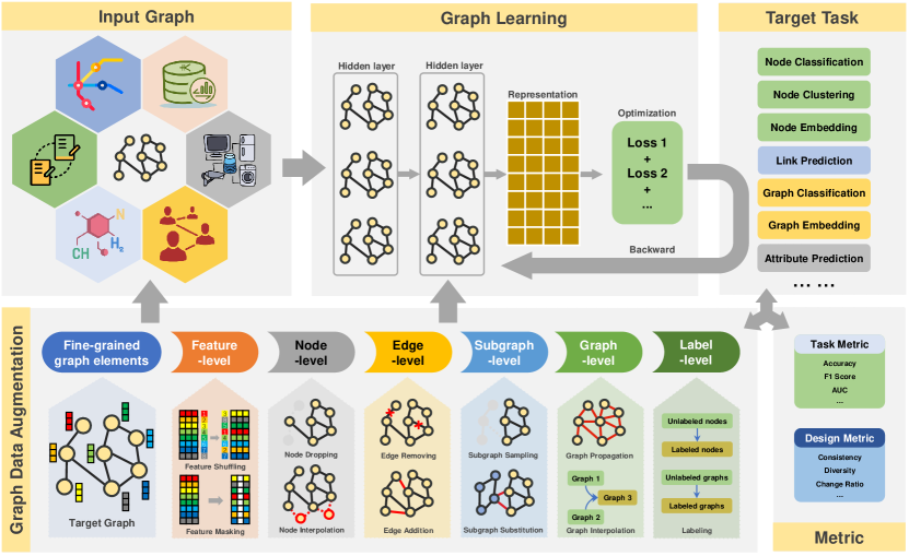
Figure 1. An overview framework of graph data augmentation with its application in graph learning.

4. Techniques of Graph Data Augmentation

Given graph data and target tasks, we hope to assist researchers to quickly find or design appropriate graph augmentation strategies. Referring to the above taxonomies, we will review the representative algorithms for graph data augmentation according to fine-grained graph elements, followed by several reasons: 1) The design freedom of augmentation strategies is limited by the diversity of graph elements, e.g., a graph without attributes generally cannot apply feature-level augmentations; 2) Augmentations based on different graph elements are usually suitable for different graph tasks, e.g., node-level augmentations are generally suitable for graph tasks at multiple scales (node, edge, graph), while subgraph-level augmentations are generally only suitable for graph-level tasks; 3) Taxonomy based on graph elements (or graph scales) is easier and clearer to organize than other taxonomies. To sum up, we will first divide existing GDAug  algorithms into feature-level, node-level, edge-level, subgraph-level, graph-level and label-level, and then further group them into different strategies for each category.

4.1. Feature-level Augmentation

Features are usually composed of multiple graph attributes, which are often derived from the real physical properties of the data and play an important role in graph representation learning. Graph features are available in attribute graphs and weighted graphs, and can be attached by different structure elements, such as nodes in point clouds carrying position features, edges in knowledge graphs carrying relationship information, and molecular graphs with global-level toxicological or catalytic properties. More broadly, graph embeddings or hidden features generated by graph representation learning are also graph features. Existing feature-level augmentations mainly concentrates on feature shuffling and feature masking.

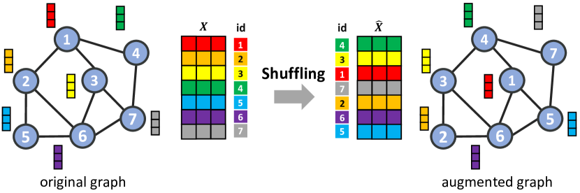
Figure 2. Illustration of feature shuffling augmentation.

4.1.1. Feature Shuffling

This strategy shuffles the graph features especially node features to generate augmented samples. Without loss of generality, we define feature shuffling as follows:

Definition 4.1.

Feature Shuffling. For a given attributed graph $G=\left(\boldsymbol{A,X_{\textit{v}}}\right)$, feature shuffling executes row-wise shuffle on the node features, yielding an augmented graph $\hat{G}=(\boldsymbol{A},\hat{\boldsymbol{X}}_{\textit{v}})$ with the same topology but rearranged nodes, i.e., 

(1) $$\hat{\boldsymbol{X}}_{\textit{v}}=\boldsymbol{X}_{\textit{v}}[\textit{idx},:]\quad\textbf{with}\quad\textit{idx}=\operatorname{Randperm}(|\mathcal{V}|)$$

where $\operatorname{Randperm}(n)$ function returns a random permutation of integers from $0$ to $|\mathcal{V}|-1$.

This augmentation is typically applied in contrastive learning to generate a diverse set of isomorphic negative samples, where the topological structure is preserved but the nodes are located in different locations and receive different contextual information, as schematically depicted in Fig. 2. DGI (Veličković et al., 2019) considers feature shuffling as a corruption function to generate negative samples for the first time, and plenty of related work (Li et al., 2022; Ren and Liu, 2020; Jing et al., 2021; Wang and Liu, 2021; Ma et al., 2021) followed suit. STDGI (Opolka et al., 2019) extends the DGI method to spatio-temporal graphs and applies feature shuffling to randomly permute the node features at each time step.

4.1.2. Feature Masking

This augmentation is also named feature perturbation and is commonly used to generate augmented graphs with masked or perturbed features. Without loss of generality, we define the generalized feature masking as follows:

Definition 4.2.

Feature Masking. For a given attributed graph $G=\left(\boldsymbol{A,X}\right)$, feature masking performs attribute-wise masking on graph features, by making the $j$-th attribute of feature vector $\boldsymbol{x}_{\textit{i}}$ masked as $m_{\textit{ij}}$ with probability $p_{\textit{ij}}^{\textit{m}}$, finally yielding an augmented graph $\hat{G}=(\boldsymbol{A},\hat{\boldsymbol{X}})$ with the same topology but masked features, i.e., 

(2) $$\hat{\boldsymbol{X}}=\boldsymbol{X}\circ\left(\boldsymbol{1}-\mathbbm{1}_{\textit{m}}\right)+\boldsymbol{M}\circ\mathbbm{1}_{\textit{m}}$$

$$\textbf{with}\quad\mathbbm{1}_{\textit{m}}[i, j]\sim\operatorname{Bernoulli}\left(p_{\textit{ij}}^{\textit{m}}\right),\quad\boldsymbol{M}[i,j]=m_{\textit{ij}}$$

where $\circ$ is the Hadamard product, $\mathbbm{1}_{\textit{m}}$ is the masking location indicator matrix, each element of $\mathbbm{1}_{\textit{m}}$ is drawn from a Bernoulli distribution with parameter $p_{\textit{ij}}^{\textit{m}}$, and $\boldsymbol{M}$ is the masking value matrix.

Table 3. Summary of different feature masking augmentations.

Reference	Strategy (custom)	Feature Masking Setting
		$p_{\textit{ij}}^{\textit{m}}$	$m_{\textit{ij}}$ / $\boldsymbol{M}$	Model Dependency
(Zhu et al., 2020; Thakoor et al., 2021, 2022; Jovanovic et al., 2021; Jin et al., 2021b; Zhou et al., 2022a; Bielak et al., 2022; Zhang et al., 2021)	uniform zero masking	constant	0	model-agnostic (random)
(You et al., 2020, 2021)	noise masking	1	$\mathcal{N}(\boldsymbol{0},\boldsymbol{\Sigma})$	model-agnostic (random)
(Wang et al., 2021a)	noise masking	1	$\mathcal{N}(\boldsymbol{X},\boldsymbol{\Sigma})$	model-agnostic (random)
(Zhu et al., 2021b)	importance-based masking	node centrality	0	model-agnostic (heuristic)
(Wang et al., 2020b)	importance-based masking	attribute weight	more relevant attributes	model-agnostic (heuristic)
(Kong et al., 2022)	gradient-based masking	1	adversarial perturbation	model-based (learnable)

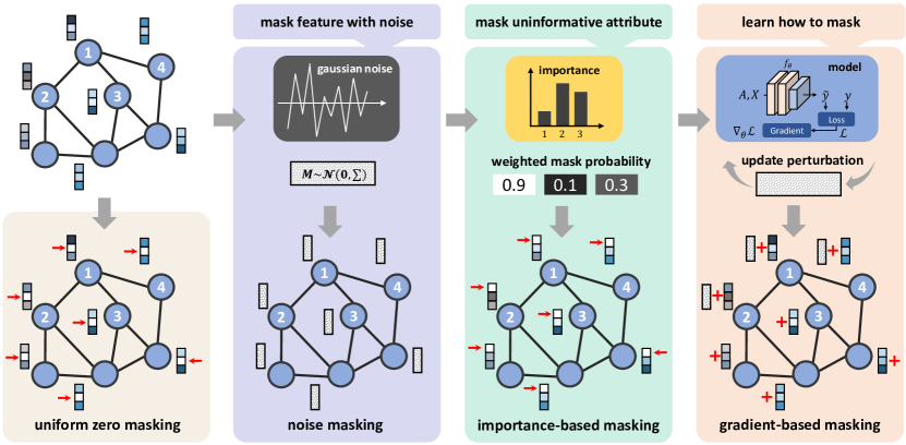
Figure 3. Illustration of different feature masking augmentations.

Note that the elements of masking matrix $\mathbbm{1}_{\textit{m}}[i,j]$ are set to 1 individually with a probability $p_{\textit{ij}}^{\textit{m}}$ and 0 with a probability $1-p_{\textit{ij}}^{\textit{m}}$. Different types of masking probabilities $p_{\textit{ij}}^{\textit{m}}$ and masking values $m_{\textit{ij}}$ specify different augmentation strategies, as shown in Table 3 and Fig. 3. For example, $p_{\textit{ij}}^{\textit{m}}$ and $m_{\textit{ij}}$ can be set to fixed constants, yielding uniform zero masking, which means uniformly masking a fraction of the dimensions with zeros in the graph features and has been widely used in (Zhu et al., 2020; Thakoor et al., 2021, 2022; Jovanovic et al., 2021; Jin et al., 2021b; Zhou et al., 2022a; Bielak et al., 2022) to generate contrastive graph views. GraphCL (You et al., 2020) utilizes a noise masking with $p_{\textit{ij}}^{\textit{m}}=1$ and $\boldsymbol{M}\sim\mathcal{N}(\boldsymbol{0},\boldsymbol{\Sigma})$ to replace the whole node feature matrix with Gaussian noise. MeTA (Wang et al., 2021a) performs timestamp perturbation by adding Gaussian noise to time attribute in edges, yielding augmented timestamps. NodeAug (Wang et al., 2020b) introduces an importance-based masking that replaces the uninformative attributes with more relevant ones, and computes the mask probabilities through attribute weights. Similarly, GCA (Zhu et al., 2021b) uses multiple node centralities to compute the mask probabilities. FLAG (Kong et al., 2022) introduces a learnable gradient-based masking and iteratively augments node features with adversarial perturbation during training. Finally, it’s worth noting that feature masking can be applied to different graph features like node features, edge features or other relevant features. For example, Ethident (Zhou et al., 2022a) uniformly masks the edge features in the Ethereum interaction graph, MeTA (Wang et al., 2021a) perturbs the timestamp attribute in edges, and SMICLR (Pinheiro et al., 2022) designs the ‘XYZ mask’ augmentation to add tiny perturbations in the atoms’ coordinates (i.e., node position features) during molecular graph representation learning.

4.2. Node-level Augmentation

Node-level augmentation mainly focuses on manipulating graph nodes to generate data diversity, and is generally applied to both node-level tasks (node interpolation, node masking) and graph-level tasks (node dropping).

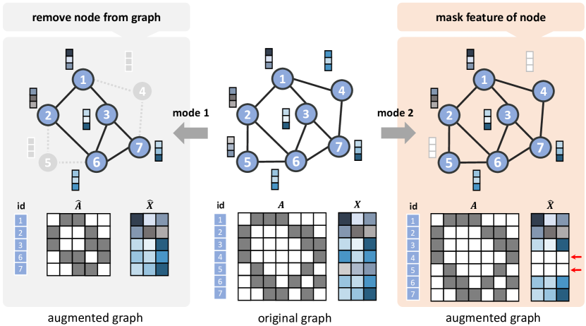
Figure 4. Illustration of node dropping augmentation. Mode 1: removing features and structure associated with selected nodes from the graph. Mode 2: masking the features of selected nodes as all-zero vectors.

4.2.1. Node Dropping

This augmentation is also named node removing, node deletion or node masking and can be regarded as a cross-class method. Without loss of generality, we define node dropping as follows:

Definition 4.3.

Node Dropping. For a given graph $G=(\boldsymbol{A},\boldsymbol{X}_{\textit{v}})$, node dropping first selects a certain proportion of nodes $\mathcal{V}_{\textit{d}}$, and then uses a corruption function $\mathcal{C}$ to deactivate them in the graph, finally yielding an augmented graph $\hat{G}$. According to the mechanism of the corruption function, node dropping can be further divided into two modes. One is to discard the selected nodes and their respective connections from the graph, i.e., 

(3) $$\hat{\boldsymbol{A}}\ ,\hat{\boldsymbol{X}}_{\textit{v}}=\mathcal{C}\left(\boldsymbol{A}\ ,\boldsymbol{X}_{\textit{v}}\right)=\boldsymbol{A}[\hat{\mathcal{V}},\hat{\mathcal{V}}]\ ,\boldsymbol{X}_{\textit{v}}[\hat{\mathcal{V}},:]$$

where $\hat{\mathcal{V}}=\mathcal{V}\setminus\mathcal{V}_{\textit{d}}$. And the other is to ignore the features of the selected nodes, i.e., 

(4) $$\hat{\boldsymbol{X}}_{\textit{v}}=\mathcal{C}\left(\boldsymbol{X}_{\textit{v}}\right)=\boldsymbol{X}_{\textit{v}}\circ\left(\boldsymbol{1}-\mathbbm{1}_{\textit{m}}\right)\quad\textbf{with}\quad\mathbbm{1}_{\textit{m}}[\mathcal{V}_{\textit{d}},:]=\boldsymbol{1},\quad\mathbbm{1}_{\textit{m}}[\hat{\mathcal{V}},:]=\boldsymbol{0}$$

where $\mathbbm{1}_{\textit{m}}$ is a masking location indicator matrix.

In mode one, node dropping is essentially a node-level graph pruning that completely removes features and structures associated with selected nodes from the graph, eventually yielding a subgraph of the original graph as an augmented sample, as schematically depicted in Fig. 4. This augmentation mode is generally applied in the graph classification task (You et al., 2020, 2021; Zeng and Xie, 2021; Pinheiro et al., 2022; Zhou et al., 2022a), and can also be regarded as subgraph sampling augmentation (as discussed in Sec. 4.4.1). As for mode two, node dropping is essentially the local node feature masking, which masks messages from selected nodes by setting their features to all-zero vectors. For example, this mode can enable a node to aggregate messages only from a subset of its neighbors, achieving an augmentation in the receptive field of the target node, and is thus widely applied in node-level tasks (Wang et al., 2021b; Park et al., 2021a; Feng et al., 2020; Sun et al., 2021b).

Table 4. Summary of different node interpolation augmentations.

Reference	Node Interpolation Setting				Adjoint edge generation?
	$\mathcal{D}_{\textit{a}}$	$\mathcal{D}_{\textit{t}}$	$\mathbbm{1}_{\textit{m}}$	$\mathcal{F}$
(Wang et al., 2021c)	$\mathcal{V}$	$\mathcal{V}$	$\boldsymbol{0}$	input / embedding spaces	False
(Verma et al., 2021)	$\mathcal{V}_{\textit{L}}$, $\mathcal{V}_{\textit{U}}$	$\mathcal{V}_{\textit{L}}$, $\mathcal{V}_{\textit{U}}$	$\boldsymbol{0}$	embedding space	False
(Xue et al., 2021)	$\mathcal{V}$	$\mathcal{V}$	$\boldsymbol{0}$	input space	True
(Park et al., 2021b)	target minority class	$\mathcal{V}_{\textit{L}}$, $\mathcal{V}_{\textit{U}}$	$\mathbbm{1}_{\textit{m}}\in\{0,1\}^{F_{\textit{v}}}$	input space	True
(Wu et al., 2022; Zhao et al., 2021b)	target minority class	$v_{\textit{t}}=\underset{v_{\textit{i}}\in\{\mathcal{V}\setminus v_{\textit{a}}\},\ y_{\textit{i}}=y_{\textit{a}}}{\operatorname{argmin}}\left\|\boldsymbol{h}_{\textit{i}}-\boldsymbol{h}_{\textit{a}}\right\|$	$\boldsymbol{0}$	embedding space	True

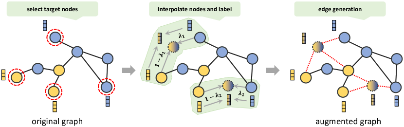
Figure 5. Illustration of generalized node interpolation augmentation.

4.2.2. Node Interpolation

This is a generative augmentation strategy that creates synthetic nodes by combining the existing nodes. Existing work based on node interpolation is mainly inspired by Mixup (Zhang et al., 2018; Verma et al., 2019) and SMOTE (Chawla et al., 2002). Mixup is a recently proposed image augmentation method based on the principle of Vicinal Risk Minimization (VRM), which can generate new synthetic images via linear interpolation. Incorporating the prior knowledge that linear interpolation of features should lead to linear interpolation of the associated targets, Mixup can extend the training distribution as follows (Zhang et al., 2018):

(5) $$\hat{\boldsymbol{x}}=(1-\lambda)\cdot\boldsymbol{x}_{\textit{i}}+\lambda\cdot\boldsymbol{x}_{\textit{j}}$$

$$\hat{{y}}=(1-\lambda)\cdot{y}_{\textit{i}}+\lambda\cdot{y}_{\textit{j}}$$

where $(\boldsymbol{x}_{\textit{i}},y_{\textit{i}})$ and $(\boldsymbol{x}_{\textit{j}},y_{\textit{j}})$ are two labeled samples sampled from training set, and $\lambda\in[0,1]$. Similarly, Manifold Mixup (Verma et al., 2019) performs mixup on the intermediate embedding space. As for SMOTE (Chawla et al., 2002), the most popular over-sampling method, it generates new samples by performing interpolation between samples in minority classes and their nearest neighbors. In some ways, SMOTE can be regarded as a special case of Mixup. After reviewing their applications in graph domain, we define the generalized node interpolation as follows:

Definition 4.4.

Node Interpolation. For a given attributed graph $G=(\boldsymbol{A},\boldsymbol{X}_{\textit{v}},\mathcal{Y}_{\textit{v}})$ and an anchor node $(v_{\textit{a}},y_{\textit{a}})\sim\mathcal{D}_{\textit{a}}$, node interpolation first samples a target node $(v_{\textit{t}},y_{\textit{t}})$ from data distribution $\mathcal{D}_{\textit{t}}$, and then combines the two nodes in the feature space $\mathcal{F}$ via generalized linear interpolation, yielding new synthetic node $\left(\hat{v},\hat{y}\right)$, i.e., 

(6) $$\hat{\boldsymbol{h}}=(1-\Lambda)\circ\boldsymbol{h}_{\textit{a}}+\Lambda\circ\boldsymbol{h}_{\textit{t}}$$

$$\hat{y}=(1-\lambda)\cdot y_{\textit{a}}+\lambda\cdot y_{\textit{t}}$$

$$\text{with}\quad\Lambda=\lambda\cdot (1-\mathbbm{1}_{\textit{m}}),\quad\boldsymbol{h}_{\textit{a}},\boldsymbol{h}_{\textit{t}}\in\mathcal{F},\quad(v_{\textit{t}},y_{\textit{t}})\sim\mathcal{D}_{\textit{t}}$$

where $\lambda\sim\operatorname{Beta}(\alpha,\alpha)$ is a random variable drawn from beta distribution, $\mathbbm{1}_{\textit{m}}$ is an optional masking location indicator vector, $\boldsymbol{h}$ is the node representation in feature space $\mathcal{F}$.

We show the general process of node interpolation in Fig. 5. Note that this definition has a slightly different form than Mixup, but is easier to encapsulate existing related work, as summarized in Table 4. Node interpolation is mainly proposed to alleviate low generalization, especially for class imbalance problem. For example, to improve class-imbalanced node classification, existing work (Park et al., 2021b; Wu et al., 2022; Zhao et al., 2021b) utilizes node interpolation to generate synthetic nodes for minority classes. In data selection, the anchor nodes are sampled from the target minority class, and the target nodes vary for different approaches. GraphMixup (Wu et al., 2022) and Graphsmote (Zhao et al., 2021b) consider the nearest neighbor of the anchor node with the same label as the target node, i.e.,

(7) $$v_{\textit{t}}=\underset{v_{\textit{i}}\in\{\mathcal{V}\setminus v_{\textit{a}}\},\ y_{\textit{i}}=y_{\textit{a}}}{\arg\min}\left\|\boldsymbol{h}_{\textit{i}}-\boldsymbol{h}_{\textit{a}}\right\|$$

In contrast, GraphENS (Park et al., 2021b) argues that selecting similar neighbors as target nodes in a highly imbalanced scenario will lead to information redundancy, so it selects target nodes from all classes, even unlabeled nodes. Regardless of the class imbalance issue, other work (Wang et al., 2021c; Verma et al., 2021; Xue et al., 2021) usually does not restrict the selection of node pairs, that is, sampling node pairs randomly from the training set.

In addition, it is worth noting that node interpolation can only generate isolated synthetic nodes, so it generally relies on an edge generation module to connect the generated nodes to the graph. For example, Graphsmote (Zhao et al., 2021b) employs a weighted inner product predictor and jointly trains it via edge reconstruction task, finally yielding binary or soft edges for synthetic nodes. Similarly, GraphMixup (Wu et al., 2022) also adopts the same edge generator but optimizes it with three self-supervised tasks: edge reconstruction, local-path prediction and global-path prediction. Moreover, GraphENS (Park et al., 2021b) first generates the adjacent node distribution for the synthetic node by mixing those of the anchor node and the target node, and then connects the synthetic node to the graph by sampling neighbors from the distribution. Two-stage Mixup (Wang et al., 2021c) does not construct an edge generator to connect synthetic nodes, but indirectly uses the adjacency information of anchor nodes and target nodes to aggregate messages for synthetic nodes. As an exception, GraphMix (Verma et al., 2021) trains a fully-connected network jointly with GNN via weight sharing, which can avoid message aggregation while performing interpolation-based regularization, thus eliminating edge generation.

Lastly, as a generalized definition, we perform feature interpolation using a composite parameter $\Lambda$, in which $\mathbbm{1}_{\textit{m}}$ usually serves for masking class-specific attributes of target nodes from introducing noise, as mentioned in (Park et al., 2021b). When mask is not used (i.e., $\mathbbm{1}_{\textit{m}}=\boldsymbol{0}$), $\Lambda$ degenerates to $\lambda$.

4.3. Edge-level Augmentation

Edge-level augmentation mainly focuses on manipulating the connection structure of graphs to generate data diversity, and is generally applied to node-level tasks and graph-level tasks. Existing edge-level augmentations include edge removing, edge additions and their hybrids, which we unify as edge rewiring.

4.3.1. Edge Rewiring

It is a widely used augmentation that can modify the graph structure without affecting the graph size. Edge rewiring is also named edge perturbation and consists of two parts, edge removing and edge addition. Without loss of generality, we define it as follows:

Definition 4.5.

Edge Rewiring. For a given graph $G=\left(\boldsymbol{A,X}\right)$ without considering edge features, edge rewiring removes or adds a portion of edges in $G$, by applying masks parameterized by two probabilities $p_{\textit{ij}}^{\textit{-}}$ and $p_{\textit{ij}}^{\textit{+}}$ to the adjacency matrix $\boldsymbol{A}$, finally yields an augmented graph $\hat{G}=(\hat{\boldsymbol{A}},\boldsymbol{X})$, i.e., 

(8) $$\hat{\boldsymbol{A}}=\underbrace{\boldsymbol{A}\circ\left(\boldsymbol{1}-\mathbbm{1}_{\textit{r}}\right)}_{\text{edge removing}}+\underbrace{\left(\boldsymbol{1}-\boldsymbol{A}\right)\circ\mathbbm{1}_{\textit{r}}}_{\text{edge addition}}$$

with $$\mathbbm{1}_{\textit{r}}[i,j]\sim\begin{cases}\operatorname{Bernoulli}\left(p_{\textit{ij}}^{\textit{-}}\right)&\text{if}\quad\boldsymbol{A}_{\textit{ij}}=1\vspace{1ex}\\ \operatorname{Bernoulli}\left(p_{\textit{ij}}^{\textit{+}}\right)&\text{if}\quad\boldsymbol{A}_{\textit{ij}}=0\end{cases}$$

where $\mathbbm{1}_{\textit{r}}$ is the rewiring location indicator matrix, $p_{\textit{ij}}^{\textit{-}}$ represents the probability of removing edge $e_{\textit{ij}}$ and $p_{\textit{ij}}^{\textit{+}}$ represents the probability of connecting nodes $v_{\textit{i}}$ and $v_{\textit{j}}$.

Table 5. Summary of different edge rewiring augmentations.

Reference	Strategy (custom)	Edge Rewiring Setting
		$p_{\textit{ij}}^{\textit{-}}$ and $p_{\textit{ij}}^{\textit{+}}$	Model Dependency
(You et al., 2020, 2021; Zeng and Xie, 2021; Pinheiro et al., 2022; Zhou et al., 2022a; Thakoor et al., 2021) (Veličković et al., 2019; Zhu et al., 2020; Bielak et al., 2022; Thakoor et al., 2022; Jin et al., 2021b)	uniform rewiring	constant	model-agnostic (random)
(Zhu et al., 2021b; Wang et al., 2020b; Zhou et al., 2020a, b, 2021a; Spinelli et al., 2021)	importance rewiring	weighted by feature and structure information	model-agnostic (heuristic)
(Li et al., 2022; Klicpera et al., 2019; Zhao et al., 2021a; Sun et al., 2021b)	prediction rewiring	generated by edge predictor and binarized by threshold or topk	model-agnostic (heuristic)
(Jovanovic et al., 2021; Suresh et al., 2021)	gradient-based rewiring	binarized by gradient information	model-based (learnable)
(Park et al., 2021a)	probabilistic rewiring	sampled from specific distribution	model-based (learnable)

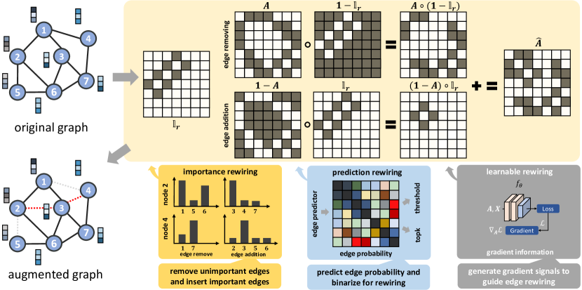
Figure 6. Illustration of different edge rewiring augmentations.

Note that elements in $\mathbbm{1}_{\textit{r}}$ with edge locations ($\boldsymbol{A}_{\textit{ij}}=1$) are set to 1 individually with probability $p_{\textit{ij}}^{\textit{-}}$ and 0 otherwise, while elements in $\mathbbm{1}_{\textit{r}}$ with non-edge locations ($\boldsymbol{A}_{\textit{ij}}=0$) are set to 1 individually with probability $p_{\textit{ij}}^{\textit{+}}$ and 0 otherwise. The first term implies edge removing where $\circ\left(\boldsymbol{1}-\mathbbm{1}_{\textit{r}}\right)$ drops edges $e_{\textit{ij}}$ if $\mathbbm{1}_{\textit{r}}[i,j]=1$, and the second term performs edge addition where $\boldsymbol{1}-\boldsymbol{A}$ represents the non-edge location indicator matrix and $\circ\mathbbm{1}_{\textit{r}}$ links node pair $(v_{\textit{i}},v_{\textit{j}})$ if $\mathbbm{1}_{\textit{r}}[i,j]=1$. In addition, when the removing probability $p_{\textit{ij}}^{\textit{-}}$ (or addition probability $p_{\textit{ij}}^{\textit{+}}$) equals to 0 for all $v_{\textit{i}},v_{\textit{j}}\in\mathcal{V}$, the edge rewiring degrades into edge addition (or edge removing).

Furthermore, different types of rewiring probabilities ($p_{\textit{ij}}^{\textit{-}}$ and $p_{\textit{ij}}^{\textit{+}}$) specify different rewiring strategies, as summarized in Table 5 and illustrated in Fig. 6. A large number of studies (Veličković et al., 2019; Zhu et al., 2020; Bielak et al., 2022; You et al., 2020, 2021; Zeng and Xie, 2021; Pinheiro et al., 2022; Zhou et al., 2022a; Thakoor et al., 2021, 2022; Jin et al., 2021b) related to graph contrastive learning typically use uniform edge rewiring to generate contrastive graph views, in which the rewiring probabilities are generally set as fixed constants. Rong et al.  (Rong et al., 2020) proposed DropEdge and its layer-wise version to alleviate over-smoothing in node representation learning. The former generates perturbed adjacency matrix via random edge removing and shares it with all layers in the GNN models, while the latter independently generates perturbed adjacency matrix for each layers. Similar to feature masking, rewiring strategies can also be designed in an importance-based manner. The rewiring probabilities can be weighted according to different information such as node centrality (Zhu et al., 2021b; Wang et al., 2020b), node similarity (Zhou et al., 2020a, b, 2021a), hop count (Wang et al., 2020b), sensitive attribute (Spinelli et al., 2021), etc. For example, NodeAug (Wang et al., 2020b) considers that nodes with larger degree values and closer distance to the target node contain more information, and further weights the rewiring probabilities by node degree and hop count. In addition, several studies first compute the edge probability matrix via different edge prediction strategies like node similarity (Li et al., 2022), graph diffusion (Klicpera et al., 2019) and graph auto-encoder (GAE) (Zhao et al., 2021a; Sun et al., 2021b), and further achieve edge rewiring via threshold-$\epsilon$ (Klicpera et al., 2019) or top-$k$ (Li et al., 2022; Klicpera et al., 2019; Zhao et al., 2021a; Sun et al., 2021b). For example, GAUG (Zhao et al., 2021a) considers graph auto-encoder (GAE) as the edge predictor to generate the edge probability matrix, and then removes the top-$k$ existing edges with least edge probabilities and adds the top-$k$ non-edges with largest edge probabilities.

The above studies are generally regarded as model-agnostic methods, and this augmentation can also be coupled with graph learning models, yielding learnable edge rewiring. GROC (Jovanovic et al., 2021) uses gradient information to guide edge rewiring, yielding an adversarial transformation that removes a portion of edges with minimal gradient values and adds a portion of edges with maximal gradient values during model training. ADGCL (Suresh et al., 2021) designs a learnable edge dropping by building a random graph model, in which each edge will be associated with a random mask variable drawn from a parametric Bernoulli distribution. MH-Aug (Park et al., 2021a) utilizes Metropolis-Hastings algorithm to sample the parameters of edge perturbation from target distribution, and then generates accepted augmented graphs via a designed acceptance ratio.

Lastly, edge removing is more commonly used than edge addition in practice. The former can be regarded as a process of graph sparsification, which can 1) denoise or prune graphs by removing misleading or uninformative links; 2) enable multiple views for random subset aggregation. The latter can restore missing links to a certain extent, but may also introduce noisy connections. In addition, when the target graph contains edge weights or attributes, edge addition augmentation needs to account for the generation of additional edge information inevitably (Wang et al., 2021a).

4.4. Subgraph-level Augmentation

Subgraph-level augmentation is generally a hybrid method because its manipulation object, the subgraph, consists of multiple graph elements. Existing methods mainly include subgraph sampling and subgraph substitution.

4.4.1. Subgraph Sampling

This one is a commonly used technique to extract substructure from a graph. Analogous to image cropping, subgraph sampling can be viewed as performing cropping on a graph, and thus can also serve for augmenting data. Here we unify existing methods, such as subgraph sampling and graph cropping, and present a generalized definition of GDAug  based on subgraph sampling:

Definition 4.6.

Subgraph Sampling. For a given graph $G=(\boldsymbol{A},\boldsymbol{X}_{\textit{v}},\boldsymbol{X}_{\textit{e}})$, subgraph sampling strategically extract node subset $\hat{\mathcal{V}}\subseteq\mathcal{V}$ and edge subset $\hat{\mathcal{E}}\subset\mathcal{E}$ from $G$ to derive an augmented subgraph $g=(\hat{\mathcal{V}},\hat{\mathcal{E}},\hat{\boldsymbol{X}}_{\textit{v}},\hat{\boldsymbol{X}}_{\textit{e}})$, where

(9) $$\hat{\boldsymbol{X}}_{\textit{v}},\ \hat{\boldsymbol{X}}_{\textit{e}}=\boldsymbol{X}_{\textit{v}}[\hat{\mathcal{V}},:],\ \boldsymbol{X}_{\textit{e}}[\hat{\mathcal{E}},:]$$

In general, subgraph sampling first determines the subset of nodes to be sampled from the graph and then determines the edge subset. This process can be guided by different sampling strategies, as summarized in Table 6 and illustrated in Fig. 7.

Table 6. Summary of different subgraph sampling augmentations.

Reference	Type (custom)	Subgraph Sampling Setting
		how to get $\hat{\mathcal{V}}$	how to get $\hat{\mathcal{E}}$ and $g$
(Hassani and Khasahmadi, 2020; Jin et al., 2021b)	uniform sampling	nodes randomly sampled from graph	$\boldsymbol{A}[\hat{\mathcal{V}},\hat{\mathcal{V}}]$
(Veličković et al., 2019; Sun et al., 2020a; Zhu et al., 2021c; Zhou et al., 2021b)	ego-net sampling	$\{v_{\textit{i}}\mid sp(v_{\textit{j}},v_{\textit{i}})\leq k\}$	$\boldsymbol{A}[\hat{\mathcal{V}},\hat{\mathcal{V}}]$
(Sun et al., 2021a; You et al., 2020)	search sampling	nodes visited by BFS/DFS starting from a node	$\boldsymbol{A}[\hat{\mathcal{V}},\hat{\mathcal{V}}]$
(You et al., 2020, 2021; Pinheiro et al., 2022; Qiu et al., 2020)	random-walk sampling	nodes visited by a random walk starting from a node	$\boldsymbol{A}[\hat{\mathcal{V}},\hat{\mathcal{V}}]$
(Zhou et al., 2022a; Jiao et al., 2020; Wang et al., 2020a; Jin et al., 2022)	importance sampling	select top-$k$ most importance neigbors for a node	$\boldsymbol{A}[\hat{\mathcal{V}},\hat{\mathcal{V}}]$
(Liu et al., 2022b)	learnable sampling	nodes selected by a learned node mask vector	$\boldsymbol{A}[\hat{\mathcal{V}},\hat{\mathcal{V}}]$
(Zheng et al., 2020)	learnable sampling	$\mathcal{V}$	sampling no more than $k$ edges for each node

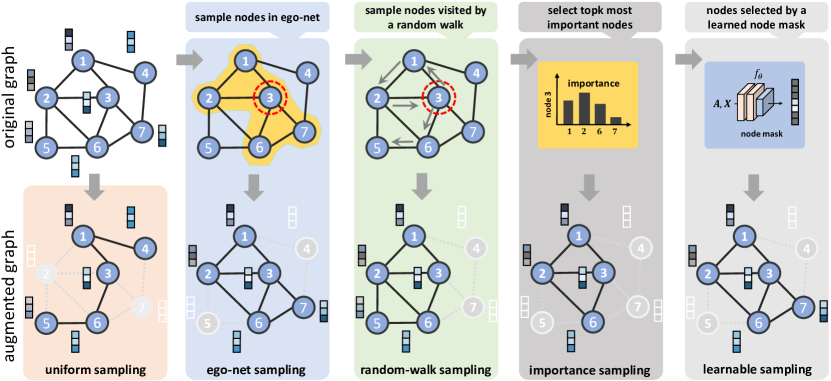
Figure 7. Illustration of different subgraph sampling augmentations.

Uniform sampling (Hassani and Khasahmadi, 2020; Jin et al., 2021b) uniformly selects a portion of nodes $\hat{\mathcal{V}}$ from $\mathcal{V}$ and then induces the subgraph topology by $\hat{\boldsymbol{A}}=\boldsymbol{A}[\hat{\mathcal{V}},\hat{\mathcal{V}}]$, which is similar to node dropping defined in Eq. (3).

Ego-net sampling is based on the strong correlation between central nodes and their local neighborhood, and is generally used to provide patch (local) views during contrastive learning, such as in DGI (Veličković et al., 2019) and InfoGraph (Sun et al., 2020a). Given a node-level encoder with $l$ layers, the computation of patch representation for node $v_{\textit{i}}$ only depends on its $l$-hop neighborhood, aka $l$-hop ego-net. A $l$-hop ego-net sampling for a central node $v_{\textit{i}}$ is essentially to obtain its receptive field subgraph with node set $\hat{\mathcal{V}}=\{v_{\textit{j}}\mid d(v_{\textit{j}},v_{\textit{i}})\leq l\}$, where $d(v_{\textit{j}},v_{\textit{i}})$ represents the shortest path distance between $v_{\textit{j}}$ and $v_{\textit{i}}$ in the graph $G$. Ego-net sampling can be regarded as a special version of Breadth-first search (BFS) sampling, which can also be used for subgraph augmentation. For example, SUGAR (Sun et al., 2021a) first selects the top-$k$ most important nodes according to degree ranking, and then extracts subgraph for each selected node by BFS sampling. GraphCL (You et al., 2020) compares the performance of contrastive learning with three kinds of subgraphs, which are extracted via BFS sampling, Depth-first search (DFS) sampling and random-walk sampling, respectively. And it concludes that the subgraphs extracted by DFS sampling preserve less structure information but help contrastive learning achieve better performance.

Random-walk sampling (You et al., 2020, 2021; Pinheiro et al., 2022; Qiu et al., 2020) is a popular strategy for extracting informative subgraphs. A random-walk sampling starting from a given node iteratively collects node subset $\hat{\mathcal{V}}$. At each iteration, the walk travels to its neighborhood with the probability proportional to the edge weight. For the random walk with restart (RWR) applied in GCC (Qiu et al., 2020), the walk has a probability of returning to the starting node.

Importance sampling (Zhou et al., 2022a; Jiao et al., 2020; Wang et al., 2020a; Zheng et al., 2020) is proposed to extract contextual subgraphs with more structure information and less noise for given nodes. For a given node, importance sampling first measures the importance scores of its neighbor nodes by several importance metrics or graph information, and then chooses the top-$k$ important neighbors to construct a subgraph. For example, SUBG-CON (Jiao et al., 2020) and GraphCrop (Wang et al., 2020a) utilize the Personalized PageRank centrality (Page et al., 1999) to measure the node importance, while Ethident (Zhou et al., 2022a) evaluates the importance of neighbors according to different edge attributes.

In addition to the above model-agnostic augmentations, several studies have proposed learnable sampling strategies to automatically extract task-relevant subgraphs. NeuralSparse (Zheng et al., 2020) trains a sparsification network to sample no more than $k$ edges for each node from a learned distribution, yielding a sparsified $k$-neighbors subgraph that preserves task-relevant edges. GREA (Liu et al., 2022b) trains a separator that maps the node representations to a mask vector, and then uses the learned node mask to extract the rationale subgraph.

4.4.2. Subgraph Substitution

Analogous to CutMix (Yun et al., 2019) that replaces the removed region with a patch from another image, subgraph substitution replaces a subgraph of the given graph with another. Here we present a generalized definition of subgraph substitution as follows:

Definition 4.7.

Subgraph Substitution. For a pair of graphs $G=(\mathcal{V},\mathcal{E},Y)$ and $G^{\textit{t}}=(\mathcal{V}^{\textit{t}},\mathcal{E}^{\textit{t}},Y^{\textit{t}})$, subgraph substitution first drops a subgraph $g=(\mathcal{V}_{\textit{g}},\mathcal{E}_{\textit{g}})$ from $G$, and then merges the remaining part with another subgraph $g^{\textit{t}}=(\mathcal{V}^{\textit{t}}_{\textit{g}},\mathcal{E}^{\textit{t}}_{\textit{g}})$ sampled from $G^{\textit{t}}$, finally yielding an augmented graph $\hat{G}=(\hat{\mathcal{V}},\hat{\mathcal{E}},\hat{Y})$, i.e., 

(10) $$\begin{array}[]{c}\hat{\mathcal{V}}=\left(\mathcal{V}\setminus\mathcal{V}_{\textit{g}}\right)\cup\mathcal{V}^{\textit{t}}_{\textit{g}}\ ,\quad\hat{\mathcal{E}}=\left(\mathcal{E}\setminus\mathcal{E}_{\textit{g}}\setminus\mathcal{E}_{\textit{break}}\right)\cup\mathcal{E}^{\textit{t}}_{\textit{g}}\cup\mathcal{E}_{\textit{connect}}\ ,\quad\hat{Y}=\left(1-\lambda\right)\cdot Y+\lambda\cdot Y^{\textit{t}}\vspace{1ex}\\ \mathcal{E}_{\textit{break}}=\left\{\left(v_{\textit{i}},v_{\textit{j}}\right)\mid\left(v_{\textit{i}},v_{\textit{j}}\right)\in\mathcal{E}\land\lnot\left(v_{\textit{i}}\in\mathcal{V}_{\textit{g}}\land v_{\textit{j}}\in\mathcal{V}_{\textit{g}}\right)\land\lnot\left(v_{\textit{i}}\in\mathcal{V}\setminus\mathcal{V}_{\textit{g}}\land v_{\textit{j}}\in\mathcal{V}\setminus\mathcal{V}_{\textit{g}}\right)\right\}\end{array}$$

where $\mathcal{E}_{\textit{break}}$ is the set of edges that break when dropping $g$ from $G$, $\mathcal{E}_{\textit{connect}}$ is the set of edges that performs merging operation to guarantee connectivity, and $\lambda$ is the adaptive label interpolation ratio.

Note that subgraph substitution is a hybrid augmentation that incorporates multiple operations like subgraph sampling, subgraph merging, and label interpolation to generate new graphs, as summarized in Table 7 and illustrated in Fig. 8. During subgraph sampling for the graph pair $(G,G^{\textit{t}})$, the two extracted substructures ($g$, $g^{\textit{t}}$) for substitution are generally of similar importance to their respective graphs, i.e., $g$ and $g^{\textit{t}}$ play similar roles in $G$ and $G^{\textit{t}}$, respectively. For example, MoCL (Sun et al., 2021c) replaces a valid substructure in a molecule with a bioisostere (Meanwell, 2011) that shares similar chemical properties. SubMix (Yoo et al., 2022) uses the importance sampling (as described in Sec. 4.4.1) to extract connected and clustered subgraphs from the given graph pair. GREA (Liu et al., 2022b) replaces the environment subgraph that can be regarded as natural noises in $G$ with another environment subgraph sampled from $G^{\textit{t}}$.

Furthermore, it is also essential to guarantee the connectivity of augmented graphs. SubMix (Yoo et al., 2022) inserts a subgraph $g^{\textit{t}}$ of the same size as $g$ into $G$ without breaking the edges that connect $\mathcal{V}_{\textit{g}}$ with $\mathcal{V}\setminus\mathcal{V}_{\textit{g}}$, having $\mathcal{E}_{\textit{connect}}=\mathcal{E}_{\textit{break}}$. Similarly, MoCL (Sun et al., 2021c) retains the chemical bonds (edges in molecular graphs) connected to $g$ before augmentation, and uses them to connect $g^{\textit{t}}$ during subgraph substitution. Graph Transplant (Park et al., 2022) proposes two strategies for merging subgraphs. One is uniform edge sampling to connect nodes whose degree values change during augmentation, and the other is differentiable edge prediction that considers the feature similarity of node pairs for connectivity. As an exception, GREA (Liu et al., 2022b) performs subgraph substitution by swapping the node representations of subgraphs in the embedding space, which is free from edge generation ($\mathcal{E}_{\textit{connect}}=\emptyset$).

Table 7. Summary of different subgraph substitution strategies.

Reference	Subgraph Substitution Setting
	Subgraph Sampling		Subgraph Merging	Label Generation
	$g$	$g^{\textit{t}}$
MoCL (Sun et al., 2021c)	valid molecular substructure	bioisostere	$\mathcal{E}_{\textit{connect}}=\mathcal{E}_{\textit{break}}$	$\lambda=0$
SubMix (Yoo et al., 2022)	connected and clustered subgraph	connected and clustered subgraph	$\mathcal{E}_{\textit{connect}}=\mathcal{E}_{\textit{break}}$	$\lambda=|\mathcal{E}^{\textit{t}}_{\textit{g}}|/|\hat{\mathcal{E}}|$
GREA (Liu et al., 2022b)	environment subgraph	environment subgraph	$\mathcal{E}_{\textit{connect}}=\emptyset$	$\lambda=0$
Graph Transplant (Park et al., 2022)	partial $l$-hop ego-net	partial $l$-hop ego net	edge sampling or prediction	subgraph saliency

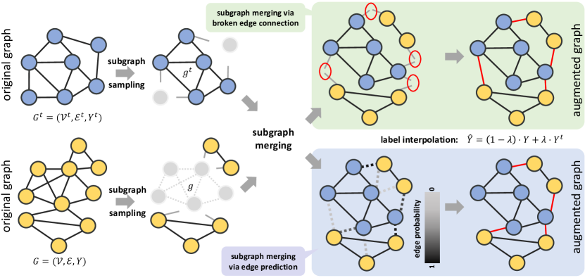
Figure 8. Illustration of generalized subgraph substitution augmentation.

Lastly, subgraph substitution generally serves for graph-level tasks, especially for graph classification, so it is necessary to assign appropriate labels for augmented graphs. Since $g$ and $g^{\textit{t}}$ play similar roles in their respective graphs, the adaptive label interpolation ratio $\lambda$ can be derived according to the contribution of $g^{\textit{t}}$ to the augmented graph $\hat{G}$. For example, SubMix (Yoo et al., 2022) assumes that edges are crucial factors in determining graph labels, and hence defines $\lambda$ as the ratio of contained edges in $g^{\textit{t}}$, i.e., $\lambda=|\mathcal{E}^{\textit{t}}_{\textit{g}}|/|\hat{\mathcal{E}}|$. Graph Transplant (Park et al., 2022) quantifies the contribution of $g^{\textit{t}}$ using the total saliency of contained nodes. In addition, both MoCL (Sun et al., 2021c) and GREA (Liu et al., 2022b) replace non-critical structures in the original graphs, so the augmented graph $\hat{G}$ and the original graph $G$ are considered to have consistent labels, i.e., $g^{\textit{t}}$ is now a non-critical subgraph and assigned a low label weight ($\lambda=0$).

4.5. Graph-level Augmentation

Graph-level augmentation mainly manipulates the graph from a global level to generate data diversity, and existing methods concentrate on graph propagation and graph interpolation.

4.5.1. Graph Propagation

This augmentation can learn global topological information from graphs through a generalized graph propagation process and generate high-order augmented views. Without loss of generality, we define it as follows:

Table 8. Summary of different graph propagation augmentations.

Algorithm	Graph Propagation Setting			Propagation equation
	$\theta_{\textit{k}}$	$\boldsymbol{T}$	$\boldsymbol{P}$
PageRank (Page et al., 1999)	$\alpha(1-\alpha)^{\textit{k}}$	$\boldsymbol{AD}^{-1}$	$\frac{1}{|\mathcal{V}|}\cdot\boldsymbol{1}$	$\boldsymbol{\Pi}=\sum_{k=0}^{\infty}\alpha(1-\alpha)^{\textit{k}}\cdot\left(\boldsymbol{AD}^{-1}\right)^{\textit{k}}\cdot\frac{1}{|\mathcal{V}|}\cdot\boldsymbol{1}=\alpha(\boldsymbol{I}-(1-\alpha)\boldsymbol{AD}^{-1})^{-1}\cdot\frac{1}{|\mathcal{V}|}\cdot\boldsymbol{1}$
Personalized PageRank (Page et al., 1999)	$\alpha(1-\alpha)^{\textit{k}}$	$\boldsymbol{AD}^{-1}$	personalized $\boldsymbol{P}_{\textit{i}}$	$\boldsymbol{\Pi}=\sum_{k=0}^{\infty}\alpha(1-\alpha)^{\textit{k}}\cdot\left(\boldsymbol{AD}^{-1}\right)^{\textit{k}}\cdot\boldsymbol{P}^{\top}=\alpha(\boldsymbol{I}-(1-\alpha)\boldsymbol{AD}^{-1})^{-1}\cdot\boldsymbol{P}^{\top}$
Heat Kernel (Chung, 2007)	$e^{\textit{-t}}\cdot\frac{t^{\textit{k}}}{k!}$	$\boldsymbol{AD}^{-1}$	identity matrix $\boldsymbol{I}$	$\boldsymbol{\Pi}=\sum_{k=0}^{\infty}e^{\textit{-t}}\cdot\frac{t^{\textit{k}}}{k!}\cdot\left(\boldsymbol{AD}^{-1}\right)^{\textit{k}}=\exp\left(t\boldsymbol{AD}^{-1}-t\right)$
Katz-index (Katz, 1953)	$\beta^{\textit{k}}$	$\boldsymbol{A}$	identity matrix $\boldsymbol{I}$	$\boldsymbol{\Pi}=\sum_{k=1}^{\infty}\beta^{\textit{k}}\boldsymbol{A}^{\textit{k}}=(\boldsymbol{I}-\beta\boldsymbol{A})^{-1}\cdot\beta\boldsymbol{A}$

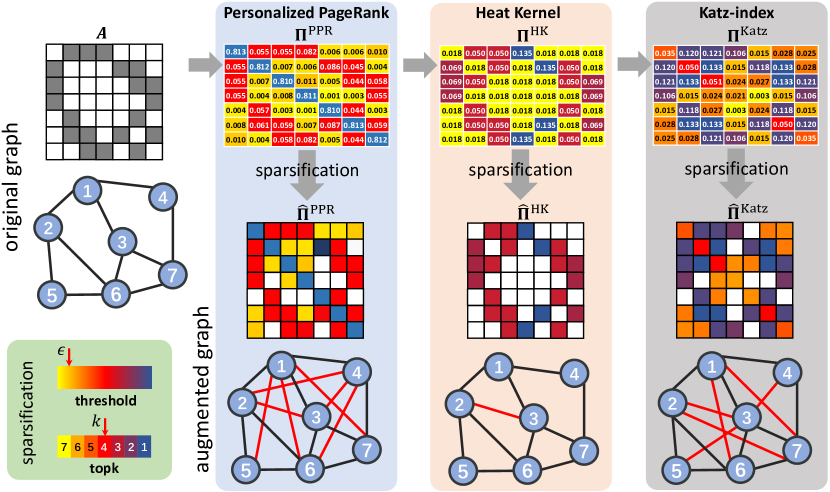
Figure 9. Illustration of different graph propagation augmentations.

Definition 4.8.

Graph Propagation. For a given graph $G=\left(\boldsymbol{A,X}\right)$, graph propagation measures the proximity between any two nodes from the perspective of global probabilistic transition, and injects high-order topological information into the graph adjacency, yielding an augmented global view $\hat{G}=(\hat{\boldsymbol{\Pi}},\boldsymbol{X})$, i.e., 

(11) $$\boldsymbol{\Pi}=\sum_{k=0}^{\infty}\theta_{\textit{k}}\cdot\boldsymbol{T}^{\textit{k}}\cdot\boldsymbol{P}^{\top}$$

$$\hat{\boldsymbol{\Pi}}=\operatorname{Sparsification}{(\boldsymbol{\Pi})}$$

where $\boldsymbol{\Pi}$ is the generated propagation matrix, $\operatorname{Sparsification}(\cdot)$ is a sparsification function, $\theta_{\textit{k}}$ is the weighting coefficent that controls the ratio of global-local information, $\boldsymbol{T}\in\mathbb{R}^{|\mathcal{V}|\times|\mathcal{V}|}$ is the generalized transition matrix, $\boldsymbol{P}\in\mathbb{R}^{|\mathcal{V}|\times|\mathcal{V}|}$ is formed by stacking the teleport location probability distribution vectors of all nodes and satisfies $\left\lVert\boldsymbol{P}_{\textit{i}}\right\rVert_{2}=1$ for all $v_{\textit{i}}\in\mathcal{V}$.

Here we summarize several graph propagation instantiations specified by different parameter settings, as listed in Table 8 and illustrated in Fig. 9. An earlier study has shown that employing higher-order message propagation mechanisms can significantly improve the performance of graph learning (Klicpera et al., 2019), which inspired the use of generalized graph diffusion methods such as Personalized PageRank (PPR) (Page et al., 1999) and Heat Kernel (HK) (Chung, 2007) to generate higher-order augmented views (Hassani and Khasahmadi, 2020; Yuan et al., 2021; Kefato and Girdzijauskas, 2021; Jin et al., 2021b). The graph diffusion powered by Personalized PageRank (PPR) is defined by setting $\boldsymbol{T}=\boldsymbol{AD}^{-1}$ and $\theta_{\textit{k}}=\alpha(1-\alpha)^{\textit{k}}$, and Heat Kernel (HK) corresponds to choosing $\boldsymbol{T}=\boldsymbol{AD}^{-1}$ and $\theta_{\textit{k}}=e^{\textit{-t}}\cdot\frac{t^{\textit{k}}}{k!}$, formulated as follows:

(12) $$\boldsymbol{\Pi}^{\text{PPR}}=\sum_{k=0}^{\infty}\alpha(1-\alpha)^{\textit{k}}\cdot\left(\boldsymbol{AD}^{-1}\right)^{\textit{k}}\cdot\boldsymbol{P}^{\top}=\alpha(\boldsymbol{I}-(1-\alpha)\boldsymbol{AD}^{-1})^{-1}\cdot\boldsymbol{P}^{\top}$$

$$\boldsymbol{\Pi}^{\text{HK}}=\sum_{k=0}^{\infty}e^{\textit{-t}}\cdot\frac{t^{\textit{k}}}{k!}\cdot\left(\boldsymbol{AD}^{-1}\right)^{\textit{k}}=\exp\left(t\boldsymbol{AD}^{-1}-t\right)$$

where $\alpha\in(0,1)$ is the tunable teleport probability in random walk, and $t$ denotes the diffusion time. Notably, compared to teleport operation with equal probability in PageRank ($\boldsymbol{P}=\frac{1}{|\mathcal{V}|}\cdot\boldsymbol{1}$), PPR is special in that each node has a user-defined (personalized) teleport location probability distribution $\boldsymbol{P}_{\textit{i}}$. In addition, SelfGNN (Kefato and Girdzijauskas, 2021) also uses the Katz-index (Katz, 1953) to capture high-order topological information and generates augmented views. The Katz-index characterizes the relative importance of nodes from a global perspective by weighting and integrating the reachable paths of different lengths between nodes. We unify it into the generalized graph propagation formula by setting $\boldsymbol{T}=\boldsymbol{A}$ and $\theta_{\textit{k}}=\beta^{\textit{k}}$, formulated as follows:

(13) $$\boldsymbol{\Pi}^{\text{Katz}}=\sum_{k=1}^{\infty}\beta^{k}\boldsymbol{A}^{k}=(\boldsymbol{I}-\beta\boldsymbol{A})^{-1}\cdot\beta\boldsymbol{A}$$

where $\beta$ is the attenuation factor that controls the path weights.

Finally, it is worth noting that the graph propagation augmentation will yield a dense propagation matrix $\boldsymbol{\Pi}$ (Klicpera et al., 2019), in which the elements represent the influence between all pairs of nodes. To guarantee the sparsity of final augmented graph, there are two tricks in practice: 1) threshold-$\epsilon$, which sets elements below $\epsilon$ to zero; 2) top-$k$, which keeps the $k$ elements with the largest values per column. Both of two sparsification tricks help to truncate small values in $\boldsymbol{\Pi}$, yielding a sparse propagation matrix $\hat{\boldsymbol{\Pi}}$ that can provide a global view during contrastive learning.

4.5.2. Graph Interpolation

This one aims to create synthetic graphs by combining the existing graphs via linear interpolation. Compared with node interpolation, graph interpolation can be more intuitively analogous to Mixup (Zhang et al., 2018) in CV. Existing work (Zhang et al., 2018; Verma et al., 2019; Zhang et al., 2020) has demonstrated that Mixup can work well on regular, well-aligned and Euclidean data such as images. However, the success of Mixup on image augmentation is difficult to reproduce in the graph domain due to the irregular structure of graph data. Currently, graph-level interpolation is relatively less explored. Here we just present a rough definition of graph interpolation:

Definition 4.9.

Graph Interpolation. For a pair of graphs $G_{\textit{i}}=(\boldsymbol{A}_{\textit{i}},\boldsymbol{X}_{\textit{i}},Y_{\textit{i}})$ and $G_{\textit{j}}=(\boldsymbol{A}_{\textit{j}},\boldsymbol{X}_{\textit{j}},Y_{\textit{j}})$, graph interpolation first aligns them in feature space $\mathcal{F}$ and then performs linear interpolation to yield an augmented graph $\hat{G}$ with label $\hat{Y}$, i.e., 

(14) $$\begin{array}[]{c}(\boldsymbol{G}_{\textit{i}},\boldsymbol{G}_{\textit{j}})=\mathcal{T}(G_{\textit{i}},G_{\textit{j}})\\ \hat{\boldsymbol{G}}=(1-\lambda)\cdot\boldsymbol{G}_{\textit{i}}+\lambda\cdot\boldsymbol{G}_{\textit{j}}\\ \hat{Y}=(1-\lambda)\cdot Y_{\textit{i}}+\lambda\cdot Y_{\textit{j}}\\ \end{array}$$

where $\mathcal{T}$ is a generalized transformation to algin the two graphs.

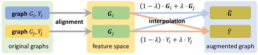
Figure 10. Illustration of generalized graph interpolation augmentation.

We review several existing related work and illustrates the generalized graph interpolation augmentation in Fig. 10. For example, ifMixup (Guo and Mao, 2021) aligns the sizes of two graphs by introducing isolated virtual nodes whose features are set to all-zero vector, and then interpolates nodes, edges and labels in the topological (input) space. Two-stage Mixup (Wang et al., 2021c) performs graph interpolation in the intermediate embedding space, where the aligned graph representations are generated by summarizing the node-level embeddings via Readout function. G-Mixup (Han et al., 2022) first estimates a graphon for each class of graphs, then performs interpolation in Euclidean space to generate mixed graphons, and finally augments synthetic graphs by sampling from the mixed graphons.

4.6. Label-level Augmentation

Most of the above-mentioned GDAug  strategies mainly manipulate the features and structure of existing graphs to achieve augmentation, without specific constraints on labels. While label-level augmentation is another important techniques used to augment the limited labeled data using the unlabeled data. We divide the existing label-level augmentations into pseudo-labeling and sharpening-labeling.

4.6.1. Pseudo-Labeling

This strategy is generally regarded as a semi-supervised method to augment the limited labeled data by generating pseudo-labels for unlabeled data. It is commonly used in conjunction with self-training (Yarowsky, 1995; Xie et al., 2020) and co-training (Blum and Mitchell, 1998). Here we present the following generalized definition of pseudo-labeling:

Definition 4.10.

Pseudo-Labeling. For a given partially labeled dataset $\mathcal{D}=\mathcal{D}_{\textit{l}}\cup\mathcal{D}_{\textit{u}}$ that can be split into a labeled set $\mathcal{D}_{\textit{l}}=\left\{(\boldsymbol{x}_{\textit{i}}^{\textit{l}},y_{\textit{i}}^{\textit{l}})\right\}_{i=1}^{|\mathcal{D}_{\textit{l}}|}$ and an unlabeled set $\mathcal{D}_{\textit{u}}=\left\{\boldsymbol{x}_{\textit{i}}^{\textit{u}}\right\}_{i=1}^{|\mathcal{D}_{\textit{u}}|}$, pseudo-labeling first trains a predictor using the partially labeled dataset, then generates pseudo labels for the unlabeled set, and finally filters out the pseudo labels with high confidence as the augmented labeled set $\hat{\mathcal{D}}_{\textit{l}}$, i.e., 

(15) $$\begin{array}[]{c}f:\mathcal{D}\rightarrow\mathbb{R}^{\textit{c}},\quad\mathcal{Y}_{\textit{u}}=f(\mathcal{D}_{\textit{u}})\vspace{1ex}\\ \mathcal{D}_{\textit{p}}=\operatorname{LabelFilter}(\mathcal{D}_{\textit{u}},\mathcal{Y}_{\textit{u}})=\left\{(\boldsymbol{x}_{\textit{i}}^{\textit{u}},y_{\textit{i}}^{\textit{u}})\mid\boldsymbol{x}_{\textit{i}}^{\textit{u}}\in\mathcal{D}_{\textit{u}},y_{\textit{i}}^{\textit{u}}\in\mathcal{Y}_{\textit{u}}\right\}_{i=1}^{K}\vspace{1ex}\\ \hat{\mathcal{D}}_{\textit{l}}=\mathcal{D}_{\textit{l}}\cup\mathcal{D}_{\textit{p}}\end{array}$$

where $f$ is the pre-trained label predictor, $\mathcal{Y}_{\textit{u}}$ is the predictive labels of unlabeled set, $\operatorname{LabelFilter}$ is a process of filtering the pseudo labels with high confidence, $\mathcal{D}_{\textit{p}}$ is the retained pseudo-labeled set of size $K$ and $1\leqslant K\leqslant|\mathcal{D}_{\textit{u}}|$.

Table 9. Summary of different label-level augmentations.

Reference	Type (custom)	Label-level Augmentation Setting
		Pseudo label generation for unlabeled data $\boldsymbol{x}^{\textit{u}}$	Label filtering $\mathcal{F}$
M-Evolve (Zhou et al., 2020b)	threshold-based	same as the original graph	threshold
AutoGRL (Sun et al., 2021b)	threshold-based	label propagation algorithm (LPA) (Zhou et al., 2003)	threshold
NRGNN (Dai et al., 2021)	threshold-based	semi-supervised prediction	threshold
CGCN (Hui et al., 2020)	clustering-based	pass the label of the labeled node to it in the same cluster	match the prediction
M3S (Sun et al., 2020b)	clustering-based	assign the label of the nearest cluster of labeled nodes to the cluster it locates	match the prediction
GraphMix (Verma et al., 2021)	sharpening	apply sharpening to the average predictions across multiple perturbations of it	/
GRAND (Feng et al., 2020)	sharpening	apply sharpening to the average predictions across multiple augmentations of it	/
NASA (Bo et al., 2022)	sharpening	apply sharpening to the average of its neighbors’ predictions	/

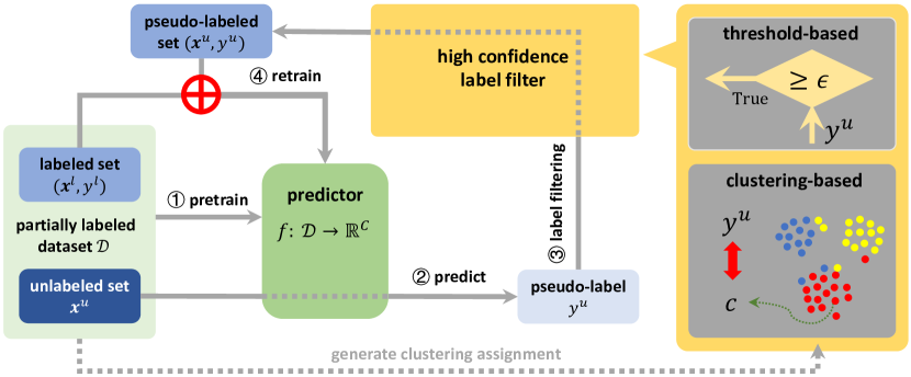
Figure 11. Illustration of pseudo-labeling augmentation. The general workflow proceeds as follows: 1) pre-train predictor using the partially labeled dataset; 2) predict the pseudo labels for unlabeled data using predictor; 3) filter the pseudo labels with high confidence; 4) retrain the predictor using the augmented set.

After pseudo-labeling, the augmented set $\hat{\mathcal{D}}_{\textit{l}}$ can be used to retrain the predictor or train a new model. And the process of pseudo-labeling and model training can go through multiple rounds. We summarize several graph related works using pseudo-labeling techniques and divide them into two categories, as listed in Table 9 and illustrated in Fig. 11. The threshold-based methods mainly construct pseudo-labels via model predictions and determine whether a pseudo-labeled sample has high confidence by comparing the model prediction probability with a threshold. M-Evolve (Zhou et al., 2020b) first generates the virtual graphs via edge rewiring and assigns them the labels of the original graphs as pseudo-labels. Then a concept of label reliability is introduced based on the intuition that pseudo-labels generally have higher reliability when matched to predictions. M-Evolve finally uses the label reliability threshold to filter out the virtual graphs with high label reliability as the augmented data. NRGNN (Dai et al., 2021) first inserts the missing edges between labeled and unlabeled nodes through edge prediction, then trains a GNN model on the rewired graph and uses the predictions of unlabeled nodes as their pseudo-labels, and finally retains the unlabeled nodes with their pseudo-labels whose predicted probability is greater than a threshold as augmented data. The clustering-based methods mainly use cluster assignments as pseudo-labels by introducing unsupervised clustering tasks, and then filter pseudo-labeled samples with high confidence by matching the consistency of supervised predictions and cluster assignments. M3S (Sun et al., 2020b) first runs K-means clustering on the node embeddings, then aligns labeled and unlabeled clusters by comparing the distance of centroids between clusters, and finally passes the label of the labeled cluster to the nearest unlabeled cluster. CGCN (Hui et al., 2020) first learns clusters by GMM-VGAE model, then select the highest confidence (softmax prediction score) labeled sample of each class, and finally passes their labels to the unlabeled nodes in the clustering network.

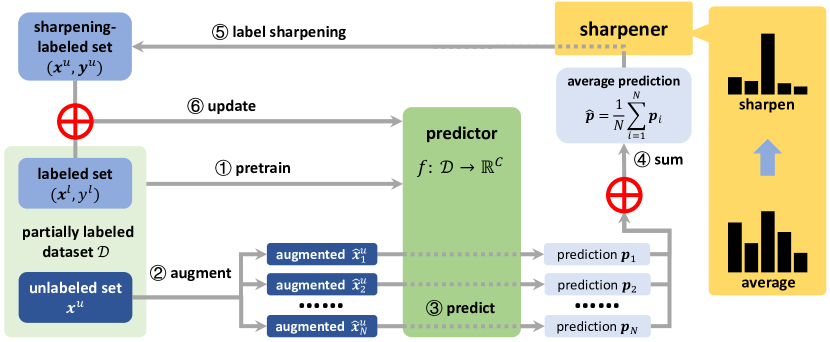
Figure 12. Illustration of sharpening-labeling augmentation. The general workflow proceeds as follows: 1) pre-train predictor using the partially labeled dataset; 2) generate $N$ augmentations of unlabeled data; 3) generate predicted probability distributions across $N$ augmentations via predictor; 4) compute the average prediction distribution; 5) apply sharpening function to generate sharpened label for unlabeled data; 6) update the predictor using the augmented set.

4.6.2. Sharpening-Labeling

Pseudo-labeling techniques are obsessed with generating high-confidence pseudo-labels for unlabeled data, which usually fail when unlabeled data has low-confidence predictions. While sharpening-labeling does not rely on high-confidence predictions and is suitable for more unlabeled scenarios. Here we present the definition of sharpening-labeling as follows:

Definition 4.11.

Sharpening-Labeling. Given predicted probability distributions $\left\{\boldsymbol{p}_{\textit{i}}\right\}^{\textit{N}}_{i=1}$ across $N$ augmentations of $\boldsymbol{x}^{\textit{u}}$, sharpening-labeling first computes the average prediction distribution, followed by a sharpening function to generate the sharpened label of $\boldsymbol{x}^{\textit{u}}$, yielding augmented data $(\boldsymbol{x}^{\textit{u}},\boldsymbol{y}^{\textit{u}})$, i.e., 

(16) $$\hat{\boldsymbol{p}}=\frac{1}{N} \sum_{i=1}^{N}\boldsymbol{p}_{\textit{i}}=\left[\hat{p}_{1},\hat{p}_{2},\cdots,\hat{p}_{\textit{C}}\right]$$

$$y^{\textit{u}}_{\textit{k}}=\hat{p}_{\textit{k}}^{\frac{1}{T}} /\sum_{j=1}^{C}\hat{p}_{\textit{j}}^{\frac{1}{T}},\quad 1\leqslant k,j\leqslant C$$

$$\boldsymbol{y}^{\textit{u}} =\left[y^{\textit{u}}_{\textit{1}},y^{\textit{u}}_{\textit{2}},\cdots,y^{\textit{u}}_{\textit{C}}\right]$$

where $\hat{\boldsymbol{p}}$ is the average prediction distribution, $C$ is the number of classes, and $T$ is the temperature hyperparameter.

The process of sharpening-labeling is illustrated in Fig. 12. Note that in practice, we usually choose temperature sharpening (LeCun et al., 2015) as the sharpening function to reduce the entropy of the prediction distribution. It is commonly used in conjunction with consistency regularization (Bo et al., 2022; Verma et al., 2021; Feng et al., 2020). Related work of sharpening-labeling is summarized in Table 9. GraphMix (Verma et al., 2021) applies the average prediction on multiple random perturbations of an input unlabeled sample along with sharpening trick, further augments training data and improve prediction accuracy. GRAND (Feng et al., 2020) utilizes sharpening-labeling to construct labels for unlabeled nodes based on the average prediction over multiple data augmentation, and further assists the implementation of consistency regularization. NASA (Bo et al., 2022) proposes a neighbor-constrained regularization to enforce the predictions of neighbors to be consistent with each other, in which the sharpening trick is used to generate label for the center node based on the average predictions of its neighbors.

Table 10. Summary of existing GDAug works. GDAug categories: FS: Feature Shuffling; FM: Feature Masking; ND: Node Dropping; NI: Node Interpolation; ER: Edge Rewiring; SSa: Subgraph Sampling; SSu: Subgraph Substitution; GP: Graph Propagation; GI: Graph Interpolation; PL: Pseudo-Labeling; SL: Sharpening-Labeling.

Ref	Model	Publication	Year	GDAug	Code
(Veličković et al., 2019)	DGI	ICLR	2019	FS, ER	https://github.com/PetarV-/DGI
(Opolka et al., 2019)	STDGI	ICLR-workshop	2019	FS	—
(Li et al., 2022)	STABLE	KDD	2022	FS, ER	—
(Jing et al., 2021)	HDMI	WWW	2021	FS	https://github.com/baoyujing/HDMI
(Ren and Liu, 2020)	HDGI	AAAI-workshop	2020	FS	https://github.com/YuxiangRen/Heterogeneous-Deep-Graph-Infomax
(Wang and Liu, 2021)	HTC	Arxiv	2021	FS	—
(Ma et al., 2021)	Contrast-Reg	Arxiv	2021	FS	—
(Kong et al., 2022)	FLAG	CVPR	2022	FM	https://github.com/devnkong/FLAG
(Zhou et al., 2022a)	Ethident	IEEE-TIFS	2022	FM, ND, ER, SSa	https://github.com/jjzhou012/Ethident
(Pinheiro et al., 2022)	SMICLR	JCIM	2022	FM, ND, ER, SSa	https://github.com/CIDAG/SMICLR
(You et al., 2020)	GraphCL	NeurIPS	2020	FM, ND, ER, SSa	https://github.com/Shen-Lab/GraphCL
(You et al., 2021)	JOAO	ICML	2021	FM, ND, ER, SSa	https://github.com/Shen-Lab/GraphCL_Automated
(Sun et al., 2021b)	AutoGRL	IJCNN	2021	FM, ND, ER, PL	https://github.com/JunweiSUN/AutoGRL
(Hassani and Khasahmadi, 2022)	LG2AR	Arxiv	2022	FM, ND, ER, SSa	—
(Zhu et al., 2020)	GRACE	ICML-workshop	2020	FM, ER	https://github.com/CRIPAC-DIG/GRACE
(Zhu et al., 2021b)	GCA	WWW	2021	FM, ER	https://github.com/CRIPAC-DIG/GCA
(Thakoor et al., 2021)	BGRL	ICLR-workshop	2021	FM, ER	https://github.com/nerdslab/bgrl
(Thakoor et al., 2022)	BGRL	ICLR	2022	FM, ER	https://github.com/Namkyeong/BGRL_Pytorch
(Jovanovic et al., 2021)	GROC	WWW-workshop	2021	FM, ER	—
(Bielak et al., 2022)	GBT	KBS	2022	FM, ER	https://github.com/pbielak/graph-barlow-twins
(Wang et al., 2020b)	NodeAug	KDD	2020	FM, ER	—
(Wang et al., 2021a)	MeTA	NeurIPS	2021	FM, ER	—
(Jin et al., 2021b)	MERIT	IJCAI	2021	FM, ER, GP	https://github.com/GRAND-Lab/MERIT
(Wang et al., 2021b)	HeCo	KDD	2021	ND	https://github.com/liun-online/HeCo
(Feng et al., 2020)	GRAND	NeurIPS	2020	ND	https://github.com/THUDM/GRAND
(Park et al., 2021a)	MH-Aug	NeurIPS	2021	ND, ER	https://github.com/hyeonzini/Metropolis-Hastings-Data-Augmentation-for-Graph-Neural-Networks
(Zeng and Xie, 2021)	CSSL	AAAI	2021	ND, ER	https://github.com/UCSD-AI4H/GraphSSL
(Wang et al., 2021c)	two-branch Mixup	WWW	2021	NI, GI	https://github.com/vanoracai/MixupForGraph
(Verma et al., 2021)	GraphMix	AAAI	2021	NI, SL	https://github.com/vikasverma1077/GraphMix
(Zhao et al., 2021b)	GraphSMOTE	WSDM	2021	NI	https://github.com/TianxiangZhao/GraphSmote
(Park et al., 2021b)	GraphENS	AAAI	2022	NI	https://github.com/JoonHyung-Park/GraphENS
(Xue et al., 2021)	NodeAug-INS	CDS	2021	NI	—
(Wu et al., 2022)	GraphMixup	ECML-PKDD	2021	NI	https://github.com/LirongWu/GraphMixup
(Zhou et al., 2022b)	AugAN	Arxiv	2022	NI	—
(Rong et al., 2020)	DropEdge	ICLR	2020	ER	https://github.com/DropEdge/DropEdge
(Zhao et al., 2021a)	GAUG	AAAI	2021	ER	https://github.com/zhao-tong/GAug
(Zhou et al., 2021a)	RobustECD	IEEE-TKDE	2021	ER	https://github.com/jjzhou012/RobustECD
(Spinelli et al., 2021)	FairDrop	IEEE TAI	2021	ER	https://github.com/ispamm/FairDrop
(Suresh et al., 2021)	AD-GCL	NeurIPS	2021	ER	https://github.com/susheels/adgcl
(Hou et al., 2020)	AdaEdge	AAAI	2020	ER	https://github.com/victorchen96/MadGap
(Luo et al., 2021)	PTDNet	WSDM	2021	ER	https://github.com/flyingdoog/PTDNet
(Zhou et al., 2020b)	M-Evolve	IEEE-TNSE	2020	ER, PL	—
(Sun et al., 2021a)	SUGAR	WWW	2021	SSa	https://github.com/RingBDStack/SUGAR
(Qiu et al., 2020)	GCC	KDD	2020	SSa	https://github.com/THUDM/GCC
(Jiao et al., 2020)	SUBG-COM	ICDM	2020	SSa	https://github.com/yzjiao/Subg-Con
(Wang et al., 2020a)	GraphCrop	Arxiv	2020	SSa	—
(Sun et al., 2020a)	InfoGraph	ICLR	2020	SSa	https://github.com/fanyun-sun/InfoGraph
(Zhu et al., 2021c)	EGI	NeurIPS	2021	SSa	https://github.com/GentleZhu/EGI
(Zheng et al., 2020)	NeuralSparse	ICML	2020	SSa	https://github.com/flyingdoog/PTDNet/tree/main/NeuralSparse
(Hassani and Khasahmadi, 2020)	MVGRL	ICML	2020	SSa, GP	https://github.com/kavehhassani/mvgrl
(Yoo et al., 2022)	SubMix	WWW	2022	SSu	https://github.com/snudatalab/GraphAug
(Park et al., 2022)	Graph Transplant	AAAI	2022	SSu	https://github.com/shimazing/Graph-Transplant
(Sun et al., 2021c)	MoCL	KDD	2021	SSu	https://github.com/illidanlab/MoCL-DK
(Liu et al., 2022b)	GREA	KDD	2022	SSu	https://github.com/liugangcode/GREA
(Kefato and Girdzijauskas, 2021)	SelfGNN	WWW-workshop	2021	GP	https://github.com/zekarias-tilahun/SelfGNN
(Yuan et al., 2021)	MV-GCN	CIKM	2021	GP	—
(Klicpera et al., 2019)	GDC	NeurIPS	2019	GP	https://github.com/gasteigerjo/gdc
(Han et al., 2022)	G-mixup	ICML	2022	GI	https://github.com/ahxt/g-mixup
(Guo and Mao, 2021)	ifMixup	Arxiv	2021	GI	—
(Bo et al., 2022)	NASA	AAAI	2022	SL	https://github.com/BUPT-GAMMA/NASA
(Hui et al., 2020)	CGCN	AAAI	2020	PL	—
(Sun et al., 2020b)	M3S	AAAI	2020	PL	https://github.com/Junseok0207/M3S_Pytorch
(Dai et al., 2021)	NRGNN	KDD	2021	PL	https://github.com/EnyanDai/NRGNN

5. Evaluation Metrics and Design Guidelines

In this section, we summarize existing metrics and guidelines for evaluating or designing graph data augmentation. We first introduce several evaluation metrics that are commonly used in graph analysis tasks, and then introduce some new metrics and guidelines specifically designed for graph data augmentation.

5.1. Common Metrics

Since graph data augmentation is an auxiliary technique, existing studies usually indirectly reflect the effectiveness of GDAug  by evaluating the performance of downstream tasks. For classification tasks like node classification (Wang et al., 2021a, 2020b) and graph classification (Zhou et al., 2020a, 2022a), it is common to use accuracy-based metrics such as Accuracy, Precision, F1 score, Area Under Curve (AUC) and Average Precision (AP) for reflecting the classification performance from different perspectives. For graph representation learning (Sun et al., 2020a; Zhu et al., 2021b; Jiao et al., 2020; Hassani and Khasahmadi, 2020), the learned embeddings will be fed into the downstream classifiers or clustering algorithms, and evaluated via accuracy-based metrics as mentioned above, or clustering-based metrics such as Normalized Mutual Information (MNI) and Adjusted Rand Index (ARI). Additionally, several works apply GDAug  in pre-training task (Qiu et al., 2020) or recommender system (Wu et al., 2021b), followed evaluation with ranking-based metrics like HITS@$k$.

5.2. Specific Metrics and Design Guidelines

Besides the common metrics above, several special metrics and guidelines have been proposed to evaluate the performance of GDAug  or guide the design of GDAug. Here we present the detailed definitions and descriptions of them.

5.2.1. Change Ratio

This metric is mainly used to measure the degree of modification of graph structure and features during manipulation-based augmentation (as mentioned in Sec. 3.4). Formally, we have the following generalized definition of change ratio:

Definition 5.1.

Change Ratio. Given a graph $G=(\mathcal{V},\mathcal{E},\boldsymbol{X})$ and its augmentation $\hat{G}=(\hat{\mathcal{V}},\hat{\mathcal{E}},\hat{\boldsymbol{X}})$, the change ratio of $G$ to $\hat{G}$ is measured by the number of modified nodes (or edges, features) divided by the number of original nodes (or edges, features), i.e., 

(17) $$M_{\Delta\mathcal{V}}=(|\mathcal{V}-\hat{\mathcal{V}}|+|\hat{\mathcal{V}}-\mathcal{V}|)/|\mathcal{V}|$$

$$M_{\Delta\mathcal{E}}=(|\mathcal{E}-\hat{\mathcal{E}}|+|\hat{\mathcal{E}}-\mathcal{E}|)/|\mathcal{E}|$$

$$M_{\Delta\boldsymbol{X}}=\|\hat{\boldsymbol{x}}-\boldsymbol{x}\|_{0}/F$$

where $F$ is the dimension of feature vector, and $\|\cdot\|_{0}$ is the zero norm.

It describes the modification ratio of nodes, edges, or features before and after augmentations like node dropping (Park et al., 2021a), edge rewiring (Zhou et al., 2020b; Park et al., 2021a) and feature masking (Zhu et al., 2020), and can also be regarded as a probability hyperparameter to guide augmentations. For example, in global uniform feature masking, the probability $p^{\textit{m}}_{\textit{ij}}$ of masking an attribute is equivalent to $M_{\Delta\boldsymbol{X}}$.

5.2.2. Tradeoff in GDAug  via Consistency and Diversity

NASA (Bo et al., 2022) proposes two metrics, i.e., consistency and diversity, to measure the correctness and generalization of GDAug, respectively. We present the definition of them as follows:

Definition 5.2.

Consistency vs. Diversity. For two models $f_{\theta}$ and $\hat{f}_{\theta}$, which are trained from the training set $\mathcal{D}_{\textit{train}}$ and its augmentation $\hat{\mathcal{D}}_{\textit{train}}$ respectively, the consistency can be represented by the accuracy of augmented model $\hat{f}_{\theta}$ on validation set $\mathcal{D}_{\textit{val}}$, i.e., 

(18) $$M_{\textit{c}}=\operatorname{Acc}\left(\hat{f}_{\theta}\left(\mathcal{D}_{\textit{val}}\right),\mathcal{Y}_{\textit{val}}\right)$$

where $\mathcal{Y}_{\textit{val}}$ is the labels of validation set. And the diversity can be represented by the prediction difference between augmented model $\hat{f}_{\theta}$ and original model $f_{\theta}$ on validation set, i.e., 

(19) $$M_{\textit{d}}=\|\hat{f}_{\theta}\left(\mathcal{D}_{\textit{val}}\right)-f_{\theta}\left(\mathcal{D}_{\textit{val}}\right)\|^{2}_{\textit{F}}$$

where $\|\cdot\|_{\textit{F}}$ is the Frobenius norm.

Specifically, a lower consistency indicates that the augmentation hurts the original data distribution, but a higher consistency may not contribute well to the generalization of the model while maintaining correctness. On the other hand, a lower diversity indicates that the augmentation contributes little to the generalization of the model, while a higher diversity cannot ensure the correctness of the augmentation. Neither metric alone can fully evaluate the quality of augmentation. Therefore, NASA combines these two metrics to trade off the design of GDAug, expecting to achieve augmentation with better correctness and generalization, improve the performance of augmented models, and build generalized decision boundaries.

5.2.3. Tradeoff in GDAug  via Affinity and Diversity

Trivedi et al.  (Trivedi et al., 2022) states that augmentation should generate samples that are close enough to the original data to share task-relevant semantics, while being sufficiently different to prevent trivially similar samples. They utilize two metrics to quantify the above tradeoff, affinity and diversity, as proposed in (Gontijo-Lopes et al., 2020). We present the definition of them as follows:

Definition 5.3.

Affinity vs. Diversity. For a model $f_{\theta}$ trained from the training set $\mathcal{D}_{\textit{train}}$, the affinity can be measured by the accuracy on augmented validation set $\hat{\mathcal{D}}_{\textit{val}}$ divided by the accuracy on the original validation set $\mathcal{D}_{\textit{val}}$, i.e., 

(20) $$M_{\textit{A}}=\frac{\operatorname{Acc}(f_{\theta}(\hat{\mathcal{D}}_{\textit{val}}),\mathcal{Y}_{\textit{val}})}{\operatorname{Acc}(f_{\theta}(\mathcal{D}_{\textit{val}}),\mathcal{Y}_{\textit{val}})}$$

where $\mathcal{Y}_{\textit{val}}$ is the labels of validation set. And the diversity can be measured by the ratio of the final training loss on the augmented training set $\hat{\mathcal{D}}_{\textit{train}}$, relative to the final training loss on the original training set $\mathcal{D}_{\textit{train}}$, i.e., 

(21) $$M_{\textit{D}}=\mathbb{E}[\hat{\mathcal{L}}_{\textit{train}}]/\mathbb{E}[\mathcal{L}_{\textit{train}}]$$

Specifically, the affinity metric is used to quantify the distribution shift of the augmented data compared to the original data, with a lower affinity indicating that the augmented data is out-of-distribution for the model. On the other hand, the diversity metric quantifies how difficult it is for a model to learn from augmented data rather than original data.

5.2.4. Preserving Connectivity

Several works (Zhou et al., 2020b; Yoo et al., 2022) state that the connectivity information of a graph before and after augmentation should not be changed, as defined below.

Definition 5.4.

Preserving Connectivity. For a graph $G$ and its augmentation $\hat{G}$, $\hat{G}$ should follow the connectivity information of $G$, i.e., $\hat{G}$ should be connected if and only if $G$ is connected.

6. Applications of Graph Data Augmentation

In this section, we review and discuss how GDAug  improves graph learning from two application levels, i.e., data and model.

6.1. Data-level Application

Collecting and constructing graph-structured data on real systems usually inevitably suffers from several dilemmas, such as label scarcity, class imbalance, information redundancy, disturbing noise, etc., which directly lead to low-quality graph data and indirectly lead to poor graph learning performance. GDAug  technology has been proposed to alleviate the problems of over-fitting, weak generalization, and low fairness caused by low-quality graph data at the data level.

6.1.1. Label Scarcity

In practical scenarios, obtaining data labels requires human labor and is time-consuming and laborious, leading to the label scarcity problem. For example, labeling account types in financial transaction networks is subject to privacy restrictions due to sensitive identity information; Toxicity labeling of molecular graphs requires extensive toxicology detection experiments; Labeling documents in citation networks requires summarizing their topics in terms of their content. Graph learning methods tend to fall into over-fitting and weak generalization when working on small and sparsely labeled graph datasets. To alleviate the issue, data augmentation is a prevalent remedy that can expand data distribution and increase data diversity, achieving an improvement in the generalization power of machine learning models trained on augmented data.

Among the aforementioned GDAug  techniques, label-level augmentation combined with graph self-training works well as a general solution to improve semi-supervised graph learning when training data is limited. Specifically, graph self-training can generate high confidence pseudo labels for unlabeled data as supervision via pre-trained models trained with limited labeled data, and the augmented data with pseudo labels can be used to retrain pre-trained models or train new models. Representative works include M3S (Sun et al., 2020b), CGCN (Hui et al., 2020), NRGNN (Dai et al., 2021) and M-Evolve (Zhou et al., 2020b), as discussed in Sec. 4.6.1. Moreover, GDAug  has also been applied in graph self-supervised learning (GSSL) (Wu et al., 2021a). For contrastive GSSL, GDAug  is generally used to generate augmented views for each instance. And two views generated from the same instance are generally regarded as a positive pair, while those generated from different instances are generally regarded as a negative pair. For example, GraphCL (You et al., 2020) proposes four GDAug  strategies, including feature masking, node dropping, edge rewiring and subgraph sampling, to generate augmented views for graphs. Other representative works include GCA (Zhu et al., 2021b), MVGRL (Hassani and Khasahmadi, 2020), MERIT (Jin et al., 2021b), CSSL (Zeng and Xie, 2021), GBT (Bielak et al., 2022), etc.  For generative GSSL, it first uses GDAug  to mask partial features or structures of graph data, and then uses pretext tasks such as reconstruction to take the masked features or structures as self-supervised signals. For example, Hu et al.  (Hu et al., 2020) first masked node and edge attributes, and then used the pretext task of attribute prediction to capture the domain knowledge of molecular graphs.

6.1.2. Class Imbalance

Class imbalance is another form of label scarcity when there is an unequal distribution of classes in the training data. In other words, the labeled minority classes may have significantly fewer samples than the majority classes. This problem is extremely common in practice and can be observed in various research fields such as anomaly detection and fraud detection (Johnson and Khoshgoftaar, 2019). For example, in the financial transaction network, most accounts belong to normal users, while the number of abnormal or fraudulent accounts labeled is far less than normal accounts. Since most existing graph learning methods are mainly based on the class-balance assumption, directly training graph models on the class-imbalanced data cannot learn the features of the minority class samples well, resulting in sub-optimal performance and low fairness. To alleviate the issue in graph data, GDAug  can be used to balance the class distribution. Existing works mainly utilize node interpolation augmentation to generate synthetic nodes for minority classes, such as GraphMixup (Wu et al., 2022), GraphENS (Park et al., 2021b), and GraphSMOTE (Zhao et al., 2021b), as described in Sec. 4.2.2.

6.1.3. Structural Noise

Real-world graphs generally contain noisy and task-irrelevant edges, which will interfere with message propagation and aggregation in graph learning, resulting in sub-optimal performance. For example, automatic following of bot accounts in social networks affects the characterization of user preferences by graph algorithms; the key structures that determine a certain property of a molecule often only occupy a small part of the entire molecular graph. In this regard, edge-level augmentations are used in graph structure learning to optimize the noisy graph structure and learn more robust graph representation. For example, Luo (Luo et al., 2021) et al. proposed a learnable topological denoising network to remove task irrelevant edges, further improving the robustness and generalization of GNNs. Other representative works include NeuralSparse (Zheng et al., 2020), TO-GNN (Yang et al., 2019), RobustECD (Zhou et al., 2021a).

6.2. Model-level Application

Despite the excellent performance of graph representation lerning methods in characterizing the features of graph data, they still expose many weaknesses and limitations, such as over-smoothing on deep GNNs, vulnerability to graph adversarial attacks, and poor transferability. In this regard, the combination of GDAug  techniques and existing graph learning paradigms can alleviate these model limitations to some extent.

6.2.1. Over-smoothing

When the over-smoothing problem exists, all node representations will gradually become indistinguishable with the increase of network depth, and finally no longer relevant to the input features, resulting in vanishing gradients. Many works (Rong et al., 2020; Li et al., 2019, 2018; Hou et al., 2020) have discussed the over-smoothing phenomenon, some of them combined with GDAug  to perturb the graph topology or features, thereby alleviating the over-smoothing problem. For example, DropEdge (Rong et al., 2020) utilizes edge removing augmentation to randomly perturb the message propagation process. AdaEdge (Hou et al., 2020) utilizes adaptive edge rewiring augmentation to iteratively optimize graph topology, i.e., removing inter-class edges and adding intra-class edges based on model predictions. GRAND (Feng et al., 2020) randomly perturb the message propagation process via node feature dropping, that is, to augment the node’s receptive field during representation learning.

6.2.2. Vulnerability

GNNs have been shown to inherit the vulnerability of deep neural networks (Jin et al., 2021a), i.e., they are susceptible to being fooled by small input perturbations known as adversarial attacks. To address this problem, some works combine graph adversarial learning and GDAug  to learn robust graph representations. For example, FLAG (Kong et al., 2022) iteratively optimizes node features by using gradient-based feature masking during training, making graph models invariant to small perturbations in the input, and further improving the robustness and generalization of graph models. GROC (Jovanovic et al., 2021) uses gradient-based edge rewiring as adversarial transformation during graph contrastive learning to generate augmented views, further improving the robustness of GNNs against adversarial attacks. GraphCL (You et al., 2020) also performs adversarial experiments to show that graph contrastive learning with GDAug  can boost the robustness of GNNs under multiple evasion attacks.

6.2.3. Transferability

Existing graph representation learning methods usually train dedicated models for domain-specific data and have weak transferability to out-of-distribution data. In this regard, several existing works utilize subgraph sampling augmentations for graph pre-training and transfer learning. For example, GCC (Qiu et al., 2020) performs random-walk sampling to augment the ego-net subgraphs, and EGI (Zhu et al., 2021c) utilizes ego-net sampling and information maximization for training transferable GNNs.

7. Open Issues and Future Directions

Although GDAug  technology has attracted considerable attention and has been widely used, there are still some shortcomings and challenges in the existing research. In this section, we summarize some open issues and discuss future research directions to address them.

7.1. Comprehensive Evaluation System

Most related works mainly use some common performance metrics to evaluate the effectiveness of GDAug. However, they only measure the quality of GDAug  according to the performance of downstream tasks, lacking the interpretability of augmentation mechanisms. Although a small number of existing works (Bo et al., 2022; Trivedi et al., 2022; Gontijo-Lopes et al., 2020) propose consistency and diversity metrics to measure the correctness and generalization of GDAug, these metrics are still some combination of predictive metrics with limited interpretability. Besides, these works also utilize multiple metrics to trade-off different properties of GDAug, lacking flexibility and generalization. Therefore, it is necessary to establish a comprehensive evaluation system for GDAug  techniques.

7.2. Complex Graph Types

Most of the existing GDAug  methods are designed for plain or homogeneous attributed graphs. However, due to the complexity of real-world systems, they are usually constructed as complex graphs to maximally retain related information. For example, financial transaction scenarios can be modeled as heterogeneous graphs, transportation systems can be modeled as spatio-temporal dynamic graphs, and wikipedia data can be modeled as knowledge graphs. GDAug  techniques on these complex graphs are less studied, and the existing studies are only generalizations of the augmentation techniques on simple graphs. Therefore, designing effective graph augmentation strategies for complex graphs is worth exploring.

8. Conclusion

In this paper, we present a comprehensive survey of graph data augmentation (GDAug). Specifically, we classify GDAug  methods into six categories according to the fine-grained graph elements, i.e., feature-level, node-level, edge-level, subgraph-level, graph-level, and label-level augmentations. We then summarize several common performance metrics and specific design metrics for evaluating GDAug. Furthermore, we review and discuss the data-level and model-level applications of GDAug. Finally, we outline existing open issues as well as future directions in this field.

- (1)
- Bielak et al. (2022) Piotr Bielak, Tomasz Kajdanowicz, and Nitesh V Chawla. 2022. Graph Barlow Twins: A Self-supervised Representation Learning Framework for Graphs. Knowledge-Based Systems (2022), 109631.
- Blum and Mitchell (1998) Avrim Blum and Tom Mitchell. 1998. Combining Labeled and Unlabeled Data with Co-training. In Proceedings of the Eleventh Annual Conference on Computational Learning Theory. 92–100.
- Bo et al. (2022) Deyu Bo, Binbin Hu, Xiao Wang, Zhiqiang Zhang, Chuan Shi, and Jun Zhou. 2022. Regularizing Graph Neural Networks via Consistency-Diversity Graph Augmentations. Proceedings of the AAAI Conference on Artificial Intelligence 36 (2022), 3913–3921.
- Chawla et al. (2002) Nitesh V Chawla, Kevin W Bowyer, Lawrence O Hall, and W Philip Kegelmeyer. 2002. SMOTE: Synthetic Minority Over-sampling Technique. Journal of Artificial Intelligence Research 16 (2002), 321–357.
- Chung (2007) Fan Chung. 2007. The Heat Kernel as the Pagerank of a Graph. Proceedings of the National Academy of Sciences 104, 50 (2007), 19735–19740.
- Dai et al. (2021) Enyan Dai, Charu Aggarwal, and Suhang Wang. 2021. Nrgnn: Learning a Label Noise Resistant Graph Neural Network on Sparsely and Noisily Labeled Graphs. In Proceedings of the 27th ACM SIGKDD Conference on Knowledge Discovery and Data Mining. 227–236.
- Ding et al. (2022) Kaize Ding, Zhe Xu, Hanghang Tong, and Huan Liu. 2022. Data Augmentation for Deep Graph Learning: A Survey. ACM SIGKDD Explorations Newsletter 24, 2 (2022), 61–77.
- Feng et al. (2020) Wenzheng Feng, Jie Zhang, Yuxiao Dong, Yu Han, Huanbo Luan, Qian Xu, Qiang Yang, Evgeny Kharlamov, and Jie Tang. 2020. Graph Random Neural Networks for Semi-supervised Learning on Graphs. Advances in neural information processing systems 33 (2020), 22092–22103.
- Gontijo-Lopes et al. (2020) Raphael Gontijo-Lopes, Sylvia Smullin, Ekin Dogus Cubuk, and Ethan Dyer. 2020. Tradeoffs in Data Augmentation: An Empirical Study. In Proceedings of the 8th International Conference on Learning Representations.
- Grover and Leskovec (2016) Aditya Grover and Jure Leskovec. 2016. Node2vec: Scalable Feature Learning for Networks. In Proceedings of the 22nd ACM SIGKDD International Conference on Knowledge Discovery and Data Mining. 855–864.
- Guo and Mao (2021) Hongyu Guo and Yongyi Mao. 2021. Intrusion-free Graph Mixup. arXiv preprint arXiv:2110.09344 (2021).
- Hamilton et al. (2017) Will Hamilton, Zhitao Ying, and Jure Leskovec. 2017. Inductive Representation Learning on Large Graphs. Advances in Neural Information Processing Systems 30 (2017).
- Han et al. (2022) Xiaotian Han, Zhimeng Jiang, Ninghao Liu, and Xia Hu. 2022. G-Mixup: Graph Data Augmentation for Graph Classification. In Proceedings of the 39th International Conference on Machine Learning. PMLR, 8230–8248.
- Hassani and Khasahmadi (2020) Kaveh Hassani and Amir Hosein Khasahmadi. 2020. Contrastive Multi-view Representation Learning on Graphs. In Proceedings of the 37th International Conference on Machine Learning. PMLR, 4116–4126.
- Hassani and Khasahmadi (2022) Kaveh Hassani and Amir Hosein Khasahmadi. 2022. Learning Graph Augmentations to Learn Graph Representations. arXiv preprint arXiv:2201.09830 (2022).
- Hou et al. (2020) Yifan Hou, Jian Zhang, James Cheng, Kaili Ma, Richard T. B. Ma, Hongzhi Chen, and Ming-Chang Yang. 2020. Measuring and Improving the Use of Graph Information in Graph Neural Networks. In Proceedings of the 8th International Conference on Learning Representations.
- Hu et al. (2020) W Hu, B Liu, J Gomes, M Zitnik, P Liang, V Pande, and J Leskovec. 2020. Strategies For Pre-training Graph Neural Networks. In Proceedings of the 8th International Conference on Learning Representations.
- Hui et al. (2020) Binyuan Hui, Pengfei Zhu, and Qinghua Hu. 2020. Collaborative Graph Convolutional Networks: Unsupervised Learning Meets Semi-supervised Learning. In Proceedings of the AAAI Conference on Artificial Intelligence, Vol. 34. 4215–4222.
- Jiao et al. (2020) Yizhu Jiao, Yun Xiong, Jiawei Zhang, Yao Zhang, Tianqi Zhang, and Yangyong Zhu. 2020. Sub-Graph Contrast for Scalable Self-Supervised Graph Representation Learning. In 2020 IEEE International Conference on Data Mining (ICDM). IEEE Computer Society, 222–231.
- Jin et al. (2022) Jie Jin, Jiajun Zhou, Chengxiang Jin, Shanqing Yu, Ziwan Zheng, and Qi Xuan. 2022. Dual-Channel Early Warning Framework for Ethereum Ponzi Schemes. In China National Conference on Big Data and Social Computing. Springer, 260–274.
- Jin et al. (2021b) Ming Jin, Yizhen Zheng, Yuan-Fang Li, Chen Gong, Chuan Zhou, and Shirui Pan. 2021b. Multi-scale Contrastive Siamese Networks for Self-supervised Graph Representation Learning. In International Joint Conference on Artificial Intelligence. 1477–1483.
- Jin et al. (2021a) Wei Jin, Yaxing Li, Han Xu, Yiqi Wang, Shuiwang Ji, Charu Aggarwal, and Jiliang Tang. 2021a. Adversarial Attacks and Defenses on Graphs. SIGKDD Explor. Newsl. 22, 2 (2021), 19–34.
- Jing et al. (2021) Baoyu Jing, Chanyoung Park, and Hanghang Tong. 2021. Hdmi: High-order Deep Multiplex Infomax. In Proceedings of the Web Conference 2021. 2414–2424.
- Johnson and Khoshgoftaar (2019) Justin M Johnson and Taghi M Khoshgoftaar. 2019. Survey on Deep Learning with Class Imbalance. Journal of Big Data 6, 1 (2019), 1–54.
- Jovanovic et al. (2021) Nikola Jovanovic, Zhao Meng, Lukas Faber, and Roger Wattenhofer. 2021. Towards Robust Graph Contrastive Learning. In WWW 2021 Workshop on Self-Supervised Learning. 1–6.
- Katz (1953) Leo Katz. 1953. A New Status Index Derived from Sociometric Analysis. Psychometrika 18, 1 (1953), 39–43.
- Kefato and Girdzijauskas (2021) Zekarias Tilahun Kefato and Sarunas Girdzijauskas. 2021. Self-supervised Graph Neural Networks without Explicit Negative Sampling. In The International Workshop on Self-Supervised Learning for the Web (SSL’21), at WWW’21.
- Kipf and Welling (2017) Thomas N. Kipf and Max Welling. 2017. Semi-Supervised Classification with Graph Convolutional Networks. In Proceedings of the 5th International Conference on Learning Representations.
- Klicpera et al. (2019) Johannes Klicpera, Stefan Weißenberger, and Stephan Günnemann. 2019. Diffusion Improves Graph Learning. In Proceedings of the 33rd International Conference on Neural Information Processing Systems. 13366–13378.
- Kong et al. (2022) Kezhi Kong, Guohao Li, Mucong Ding, Zuxuan Wu, Chen Zhu, Bernard Ghanem, Gavin Taylor, and Tom Goldstein. 2022. Robust Optimization As Data Augmentation for Large-Scale Graphs. In Proceedings of the IEEE/CVF Conference on Computer Vision and Pattern Recognition. 60–69.
- LeCun et al. (2015) Yann LeCun, Yoshua Bengio, and Geoffrey Hinton. 2015. Deep Learning. Nature 521, 7553 (2015), 436–444.
- Li et al. (2019) Guohao Li, Matthias Muller, Ali Thabet, and Bernard Ghanem. 2019. Deepgcns: Can Gcns Go as Deep as Cnns?. In Proceedings of the IEEE/CVF International Conference on Computer Vision. 9267–9276.
- Li et al. (2022) Kuan Li, Yang Liu, Xiang Ao, Jianfeng Chi, Jinghua Feng, Hao Yang, and Qing He. 2022. Reliable Representations Make A Stronger Defender: Unsupervised Structure Refinement for Robust GNN. In Proceedings of the 28th ACM SIGKDD Conference on Knowledge Discovery and Data Mining. 925–935.
- Li et al. (2018) Qimai Li, Zhichao Han, and Xiao-Ming Wu. 2018. Deeper Insights into Graph Convolutional Networks for Semi-supervised Learning. In Thirty-Second AAAI Conference on Artificial Intelligence.
- Liu et al. (2022b) Gang Liu, Tong Zhao, Jiaxin Xu, Tengfei Luo, and Meng Jiang. 2022b. Graph Rationalization with Environment-Based Augmentations. In Proceedings of the 28th ACM SIGKDD Conference on Knowledge Discovery and Data Mining. 1069–1078.
- Liu et al. (2022a) Yixin Liu, Ming Jin, Shirui Pan, Chuan Zhou, Yu Zheng, Feng Xia, and Philip Yu. 2022a. Graph self-supervised learning: A survey. IEEE Transactions on Knowledge and Data Engineering (2022).
- Luo et al. (2021) Dongsheng Luo, Wei Cheng, Wenchao Yu, Bo Zong, Jingchao Ni, Haifeng Chen, and Xiang Zhang. 2021. Learning to Drop: Robust Graph Neural Network via Topological Denoising. In Proceedings of the 14th ACM International Conference on Web Search and Data Mining. 779–787.
- Ma et al. (2021) Kaili Ma, Haochen Yang, Han Yang, Tatiana Jin, Pengfei Chen, Yongqiang Chen, Barakeel Fanseu Kamhoua, and James Cheng. 2021. Improving Graph Representation Learning by Contrastive Regularization. arXiv preprint arXiv:2101.11525 (2021).
- Marrium and Mahmood (2022) Maria Marrium and Arif Mahmood. 2022. Data Augmentation for Graph Data: Recent Advancements. arXiv preprint arXiv:2208.11973 (2022).
- Meanwell (2011) Nicholas A Meanwell. 2011. Synopsis of Some Recent Tactical Application of Bioisosteres in Drug Design. Journal of Medicinal Chemistry 54, 8 (2011), 2529–2591.
- Opolka et al. (2019) Felix L Opolka, Aaron Solomon, Cătălina Cangea, Petar Veličković, Pietro Liò, and R Devon Hjelm. 2019. Spatio-temporal Deep Graph Infomax. In ICLR 2019 Workshop on Representation Learning on Graphs and Manifolds. 1–6.
- Page et al. (1999) Lawrence Page, Sergey Brin, Rajeev Motwani, and Terry Winograd. 1999. The PageRank Citation Ranking: Bringing Order to the Web. Technical Report. Stanford InfoLab.
- Park et al. (2021a) Hyeonjin Park, Seunghun Lee, Sihyeon Kim, Jinyoung Park, Jisu Jeong, Kyung-Min Kim, Jung-Woo Ha, and Hyunwoo J Kim. 2021a. Metropolis-hastings Data Augmentation for Graph Neural Networks. Advances in Neural Information Processing Systems 34 (2021), 19010–19020.
- Park et al. (2022) Joonhyung Park, Hajin Shim, and Eunho Yang. 2022. Graph Transplant: Node Saliency-guided Graph Mixup with Local Structure Preservation. In Proceedings of the First MiniCon Conference.
- Park et al. (2021b) Joonhyung Park, Jaeyun Song, and Eunho Yang. 2021b. GraphENS: Neighbor-Aware Ego Network Synthesis for Class-Imbalanced Node Classification. In Proceedings of the 9th International Conference on Learning Representations.
- Pinheiro et al. (2022) Gabriel A Pinheiro, Juarez LF Da Silva, and Marcos G Quiles. 2022. SMICLR: Contrastive Learning on Multiple Molecular Representations for Semisupervised and Unsupervised Representation Learning. Journal of Chemical Information and Modeling (2022).
- Qiu et al. (2020) Jiezhong Qiu, Qibin Chen, Yuxiao Dong, Jing Zhang, Hongxia Yang, Ming Ding, Kuansan Wang, and Jie Tang. 2020. Gcc: Graph Contrastive Coding for Graph Neural Network Pre-training. In Proceedings of the 26th ACM SIGKDD International Conference on Knowledge Discovery and Data Mining. 1150–1160.
- Ren and Liu (2020) Yuxiang Ren and Bo Liu. 2020. Heterogeneous Deep Graph Infomax. In Workshop of Deep Learning on Graphs: Methodologies and Applications co-located with the Thirty-Fourth AAAI Confer-ence on Artificial Intelligence.
- Rong et al. (2020) Yu Rong, Wenbing Huang, Tingyang Xu, and Junzhou Huang. 2020. DropEdge: Towards Deep Graph Convolutional Networks on Node Classification. In Proceedings of the 7th International Conference on Learning Representations.
- Shorten and Khoshgoftaar (2019) Connor Shorten and Taghi M Khoshgoftaar. 2019. A Survey on Image Data Augmentation for Deep Learning. Journal of Big Data 6, 1 (2019), 1–48.
- Spinelli et al. (2021) Indro Spinelli, Simone Scardapane, Amir Hussain, and Aurelio Uncini. 2021. Fairdrop: Biased Edge Dropout for Enhancing Fairness in Graph Representation Learning. IEEE Transactions on Artificial Intelligence 3, 3 (2021), 344–354.
- Sun et al. (2020a) Fan-Yun Sun, Jordon Hoffman, Vikas Verma, and Jian Tang. 2020a. InfoGraph: Unsupervised and Semi-supervised Graph-Level Representation Learning via Mutual Information Maximization. In Proceedings of the 8th International Conference on Learning Representations.
- Sun et al. (2021b) Junwei Sun, Bai Wang, and Bin Wu. 2021b. Automated Graph Representation Learning for Node Classification. In 2021 International Joint Conference on Neural Networks (IJCNN). IEEE, 1–7.
- Sun et al. (2020b) Ke Sun, Zhouchen Lin, and Zhanxing Zhu. 2020b. Multi-stage Self-supervised Learning for Graph Convolutional Networks on Graphs with Few Labeled Nodes. In Proceedings of the AAAI Conference on Artificial Intelligence, Vol. 34. 5892–5899.
- Sun et al. (2021c) Mengying Sun, Jing Xing, Huijun Wang, Bin Chen, and Jiayu Zhou. 2021c. MoCL: Data-driven Molecular Fingerprint via Knowledge-aware Contrastive Learning from Molecular Graph. In Proceedings of the 27th ACM SIGKDD Conference on Knowledge Discovery and Data Mining. 3585–3594.
- Sun et al. (2021a) Qingyun Sun, Jianxin Li, Hao Peng, Jia Wu, Yuanxing Ning, Philip S Yu, and Lifang He. 2021a. Sugar: Subgraph Neural Network with Reinforcement Pooling and Self-supervised Mutual Information Mechanism. In Proceedings of the Web Conference 2021. 2081–2091.
- Suresh et al. (2021) Susheel Suresh, Pan Li, Cong Hao, and Jennifer Neville. 2021. Adversarial Graph Augmentation to Improve Graph Contrastive Learning. Advances in Neural Information Processing Systems 34 (2021), 15920–15933.
- Thakoor et al. (2022) Shantanu Thakoor, Corentin Tallec, Mohammad Gheshlaghi Azar, Mehdi Azabou, Eva L Dyer, Remi Munos, Petar Veličković, and Michal Valko. 2022. Large-Scale Representation Learning on Graphs via Bootstrapping. In Proceedings of the 9th International Conference on Learning Representations. 1–21.
- Thakoor et al. (2021) Shantanu Thakoor, Corentin Tallec, Mohammad Gheshlaghi Azar, Rémi Munos, Petar Veličković, and Michal Valko. 2021. Bootstrapped Representation Learning on Graphs. In ICLR 2021 Workshop on Geometrical and Topological Representation Learning. 1–14.
- Trivedi et al. (2022) Puja Trivedi, Ekdeep Singh Lubana, Yujun Yan, Yaoqing Yang, and Danai Koutra. 2022. Augmentations in Graph Contrastive Learning: Current Methodological Flaws and towards Better Practices. In Proceedings of the ACM Web Conference 2022. 1538–1549.
- Veličković et al. (2019) Petar Veličković, William Fedus, William L. Hamilton, Pietro Liò, Yoshua Bengio, and R Devon Hjelm. 2019. Deep Graph Infomax. In Proceedings of the 7th International Conference on Learning Representations. 1–17.
- Verma et al. (2019) Vikas Verma, Alex Lamb, Christopher Beckham, Amir Najafi, Ioannis Mitliagkas, David Lopez-Paz, and Yoshua Bengio. 2019. Manifold Mixup: Better Representations by Interpolating Hidden States. In Proceedings of the 36th International Conference on Machine Learning. PMLR, 6438–6447.
- Verma et al. (2021) Vikas Verma, Meng Qu, Kenji Kawaguchi, Alex Lamb, Yoshua Bengio, Juho Kannala, and Jian Tang. 2021. Graphmix: Improved Training of Gnns for Semi-supervised Learning. In Proceedings of the AAAI Conference on Artificial Intelligence, Vol. 35. 10024–10032.
- Wang and Liu (2021) Chenguang Wang and Ziwen Liu. 2021. Learning Graph Representation by Aggregating Subgraphs via Mutual Information Maximization. arXiv preprint arXiv:2103.13125 (2021).
- Wang et al. (2021b) Xiao Wang, Nian Liu, Hui Han, and Chuan Shi. 2021b. Self-supervised Heterogeneous Graph Neural Network with Co-contrastive Learning. In Proceedings of the 27th ACM SIGKDD Conference on Knowledge Discovery and Data Mining. 1726–1736.
- Wang et al. (2021a) Yiwei Wang, Yujun Cai, Yuxuan Liang, Henghui Ding, Changhu Wang, Siddharth Bhatia, and Bryan Hooi. 2021a. Adaptive Data Augmentation on Temporal Graphs. Advances in Neural Information Processing Systems 34 (2021), 1440–1452.
- Wang et al. (2020a) Yiwei Wang, Wei Wang, Yuxuan Liang, Yujun Cai, and Bryan Hooi. 2020a. Graphcrop: Subgraph Cropping for Graph Classification. arXiv preprint arXiv:2009.10564 (2020).
- Wang et al. (2021c) Yiwei Wang, Wei Wang, Yuxuan Liang, Yujun Cai, and Bryan Hooi. 2021c. Mixup for Node and Graph Classification. In Proceedings of the Web Conference 2021. 3663–3674.
- Wang et al. (2020b) Yiwei Wang, Wei Wang, Yuxuan Liang, Yujun Cai, Juncheng Liu, and Bryan Hooi. 2020b. Nodeaug: Semi-supervised Node Classification with Data Augmentation. In Proceedings of the 26th ACM SIGKDD International Conference on Knowledge Discovery and Data Mining. 207–217.
- Wu et al. (2021b) Jiancan Wu, Xiang Wang, Fuli Feng, Xiangnan He, Liang Chen, Jianxun Lian, and Xing Xie. 2021b. Self-supervised Graph Learning for Recommendation. In Proceedings of the 44th International ACM SIGIR Conference on Research and Development in Information Retrieval. 726–735.
- Wu et al. (2021a) Lirong Wu, Haitao Lin, Cheng Tan, Zhangyang Gao, and Stan Z. Li. 2021a. Self-supervised Learning on Graphs: Contrastive, Generative,or Predictive. IEEE Transactions on Knowledge and Data Engineering (2021), 1–1.
- Wu et al. (2022) Lirong Wu, Jun Xia, Zhangyang Gao, Haitao Lin, Cheng Tan, and Stan Z Li. 2022. GraphMixup: Improving Class-Imbalanced Node Classification by Reinforcement Mixup and Self-supervised Context Prediction. (2022).
- Xie et al. (2020) Qizhe Xie, Minh-Thang Luong, Eduard Hovy, and Quoc V Le. 2020. Self-training With Noisy Student Improves Imagenet Classification. In Proceedings of the IEEE/CVF Conference on Computer Vision and Pattern Recognition. 10687–10698.
- Xie et al. (2022) Yaochen Xie, Zhao Xu, Jingtun Zhang, Zhengyang Wang, and Shuiwang Ji. 2022. Self-supervised learning of graph neural networks: A unified review. IEEE Transactions on Pattern Analysis and Machine Intelligence (2022).
- Xue et al. (2021) Yifan Xue, Yixuan Liao, Xiaoxin Chen, and Jingwei Zhao. 2021. Node Augmentation Methods for Graph Neural Network Based Object Classification. In 2021 2nd International Conference on Computing and Data Science (CDS). IEEE, 556–561.
- Yang et al. (2019) Liang Yang, Zesheng Kang, Xiaochun Cao, Di Jin, Bo Yang, and Yuanfang Guo. 2019. Topology Optimization based Graph Convolutional Network.. In IJCAI. 4054–4061.
- Yarowsky (1995) David Yarowsky. 1995. Unsupervised Word Sense Disambiguation Rivaling Supervised Methods. In 33rd Annual Meeting of the Association for Computational Linguistics. 189–196.
- Yoo et al. (2022) Jaemin Yoo, Sooyeon Shim, and U Kang. 2022. Model-Agnostic Augmentation for Accurate Graph Classification. In Proceedings of the Web Conference 2022. 1281–1291.
- You et al. (2021) Yuning You, Tianlong Chen, Yang Shen, and Zhangyang Wang. 2021. Graph Contrastive Learning Automated. In Proceedings of the 38th International Conference on Machine Learning. PMLR, 12121–12132.
- You et al. (2020) Yuning You, Tianlong Chen, Yongduo Sui, Ting Chen, Zhangyang Wang, and Yang Shen. 2020. Graph Contrastive Learning with Augmentations. Advances in Neural Information Processing Systems 33 (2020), 5812–5823.
- Yu et al. (2022) Shuo Yu, Huafei Huang, Minh N. Dao, and Feng Xia. 2022. Graph Augmentation Learning. In Companion Proceedings of the Web Conference 2022 (Virtual Event, Lyon, France) (WWW ’22). Association for Computing Machinery, New York, NY, USA, 1063–1072.
- Yuan et al. (2021) Jinliang Yuan, Hualei Yu, Meng Cao, Ming Xu, Junyuan Xie, and Chongjun Wang. 2021. Semi-Supervised and Self-Supervised Classification with Multi-View Graph Neural Networks. In Proceedings of the 30th ACM International Conference on Information and Knowledge Management. 2466–2476.
- Yun et al. (2019) Sangdoo Yun, Dongyoon Han, Seong Joon Oh, Sanghyuk Chun, Junsuk Choe, and Youngjoon Yoo. 2019. Cutmix: Regularization Strategy to Train Strong Classifiers with Localizable Features. In Proceedings of the IEEE/CVF International Conference on Computer Vision. 6023–6032.
- Zeng and Xie (2021) Jiaqi Zeng and Pengtao Xie. 2021. Contrastive Self-supervised Learning for Graph Classification. In Proceedings of the AAAI Conference on Artificial Intelligence, Vol. 35. 10824–10832.
- Zhang et al. (2018) Hongyi Zhang, Moustapha Cisse, Yann N Dauphin, and David Lopez-Paz. 2018. Mixup: Beyond Empirical Risk Minimization. In Proceedings of the 6th International Conference on Learning Representations.
- Zhang et al. (2021) Hengrui Zhang, Qitian Wu, Junchi Yan, David Wipf, and Philip S Yu. 2021. From Canonical Correlation Analysis to Self-supervised Graph Neural Networks. Advances in Neural Information Processing Systems 34 (2021), 76–89.
- Zhang et al. (2020) Linjun Zhang, Zhun Deng, Kenji Kawaguchi, Amirata Ghorbani, and James Zou. 2020. How Does Mixup Help With Robustness and Generalization?. In Proceedings of the 8th International Conference on Learning Representations.
- Zhao et al. (2022) Tong Zhao, Gang Liu, Stephan Günnemann, and Meng Jiang. 2022. Graph Data Augmentation for Graph Machine Learning: A Survey. arXiv preprint arXiv:2202.08871 (2022).
- Zhao et al. (2021a) Tong Zhao, Yozen Liu, Leonardo Neves, Oliver Woodford, Meng Jiang, and Neil Shah. 2021a. Data Augmentation for Graph Neural Networks. In Proceedings of the AAAI Conference on Artificial Intelligence, Vol. 35. 11015–11023.
- Zhao et al. (2021b) Tianxiang Zhao, Xiang Zhang, and Suhang Wang. 2021b. Graphsmote: Imbalanced Node Classification on Graphs with Graph Neural Networks. In Proceedings of the 14th ACM International Conference on Web Search and Data Mining. 833–841.
- Zheng et al. (2020) Cheng Zheng, Bo Zong, Wei Cheng, Dongjin Song, Jingchao Ni, Wenchao Yu, Haifeng Chen, and Wei Wang. 2020. Robust Graph Representation Learning via Neural Sparsification. In Proceedings of the 37th International Conference on Machine Learning. PMLR, 11458–11468.
- Zhou et al. (2003) Dengyong Zhou, Olivier Bousquet, Thomas Lal, Jason Weston, and Bernhard Schölkopf. 2003. Learning with Local and Global Consistency. Advances in Neural Information Processing Systems 16 (2003).
- Zhou et al. (2021a) Jiajun Zhou, Zhi Chen, Min Du, Lihong Chen, Shanqing Yu, Guanrong Chen, and Qi Xuan. 2021a. RobustECD: Enhancement of Network Structure for Robust Community Detection. IEEE Transactions on Knowledge and Data Engineering (2021).
- Zhou et al. (2022a) Jiajun Zhou, Chenkai Hu, Jianlei Chi, Jiajing Wu, Meng Shen, and Qi Xuan. 2022a. Behavior-aware Account De-anonymization on Ethereum Interaction Graph. IEEE Transactions on Information Forensics and Security 17 (2022), 3433–3448.
- Zhou et al. (2021b) Jiajun Zhou, Jie Shen, Yalu Shan, Qi Xuan, and Guanrong Chen. 2021b. Subgraph Augmentation with Application to Graph Mining. Graph Data Mining: Algorithm, Security and Application (2021), 73–91.
- Zhou et al. (2020a) Jiajun Zhou, Jie Shen, and Qi Xuan. 2020a. Data Augmentation for Graph Classification. In Proceedings of the 29th ACM International Conference on Information and Knowledge Management. 2341–2344.
- Zhou et al. (2020b) Jiajun Zhou, Jie Shen, Shanqing Yu, Guanrong Chen, and Qi Xuan. 2020b. M-evolve: Structural-mapping-based Data Augmentation for Graph Classification. IEEE Transactions on Network Science and Engineering 8, 1 (2020), 190–200.
- Zhou et al. (2022b) Shuang Zhou, Xiao Huang, Ninghao Liu, Fu-Lai Chung, and Long-Kai Huang. 2022b. Improving Generalizability of Graph Anomaly Detection Models via Data Augmentation. arXiv preprint arXiv:2209.10168 (2022).
- Zhu et al. (2021c) Qi Zhu, Carl Yang, Yidan Xu, Haonan Wang, Chao Zhang, and Jiawei Han. 2021c. Transfer Learning of Graph Neural Networks with Ego-graph Information Maximization. Advances in Neural Information Processing Systems 34 (2021), 1766–1779.
- Zhu et al. (2021a) Yanqiao Zhu, Yichen Xu, Qiang Liu, and Shu Wu. 2021a. An Empirical Study of Graph Contrastive Learning. In Thirty-fifth Conference on Neural Information Processing Systems Datasets and Benchmarks Track (Round 2).
- Zhu et al. (2020) Yanqiao Zhu, Yichen Xu, Feng Yu, Qiang Liu, Shu Wu, and Liang Wang. 2020. Deep Graph Contrastive Representation Learning. In ICML 2020 Workshop on Graph Representation Learning and Beyond. 1–9.
- Zhu et al. (2021b) Yanqiao Zhu, Yichen Xu, Feng Yu, Qiang Liu, Shu Wu, and Liang Wang. 2021b. Graph Contrastive Learning with Adaptive Augmentation. In Proceedings of the Web Conference 2021. 2069–2080.