The Late Time Optical Evolution of Twelve Core-Collapse Supernovae: Detection of Normal Stellar Winds

Abstract

We analyze the late time evolution of 12 supernovae (SNe) occurring over the last ${\sim}$41 years, including nine Type IIP/L, two IIb, and one Ib/c, using UBVR optical data from the Large Binocular Telescope (LBT) and difference imaging. We see late time (5 to 42 years) emission from nine of the eleven Type II SNe (eight Type IIP/L, one IIb). We consider radioactive decay, circumstellar medium (CSM) interactions, pulsar/engine driven emission, dust echoes, and shock perturbed binary companions as possible sources of emission. The observed emission is most naturally explained as CSM interactions with the normal stellar winds of red supergiants with mass loss rates in the range $-7.9\lesssim\log_{10}(M_{\odot}\text{yr}{}^{-1})\lesssim-4.8$. We also place constraints on the presence of any shock heated binary companion to the Type Ib/c SN 2012fh and provide progenitor photometry for the Type IIb SN 2011dh, the only one of the six SNe with pre-explosion LBT observations where the SN has faded sufficiently to allow the measurement. The results are consistent with measurements from pre-explosion Hubble Space Telescope (HST) images.

1 Introduction

For all massive stars ($>8M_{\odot}$), the end stages of stellar evolution involve the ultimate collapse of the iron core. In most cases this leads to an explosion and a luminous supernova (SN). These core-collapse supernovae (ccSNe) are categorized into sub-types based on their photometric and spectroscopic properties. To simplify the typing somewhat, Type IIP/L SN arise from red supergiants (RSG), Type Ib/c SN come from stars stripped of their envelopes, and Type IIn SN explode into a dense circumstellar medium (CSM). In the standard picture of non-Type IIn explosions, SNe can support their near peak luminosities until the ejecta recombine and become optically thin, and then the luminosity in the nebular phase is from radioactive decay. In Type IIn SNe, there is a significant or dominant contribution to the emission from shock heating the dense CSM.

As part of a search for failed SNe first proposed by Kochanek et al. (2008b), we have been monitoring 27 nearby ($<10$Mpc) galaxies to search for failed supernovae. The survey also enables two unique studies of the stars which do explode. First, it can be used to study the pre-SN variability of the progenitor stars, so far with null results almost down to the levels of the variability of local RSGs, (e.g., Szczygieł et al. 2012, Kochanek et al. 2017b, Johnson et al. 2018a). This is difficult to reconcile with claims that SN light curves require unusually high pre-SN mass loss rates (e.g., Morozova et al. (2018) and Wu & Fuller (2022) discuss many claimed examples). Second, by waiting for the SN to fade, it is possible to obtain high precision UBVR photometry of the progenitor stars using image subtraction (e.g., Johnson et al. 2017). Based on either SN 1987A (e.g., Seitenzahl et al. 2014) or typical estimates of the radioactive yields of ccSNe, this should be feasible after ${\sim}3$-$4$ years.

In the most recent search for new failed SN, Neustadt et al. (2021) noted that SN 2013am and SN 2013ej were still brighter than their progenitors a decade after explosion. This is illustrated in Fig. 1 for SN 2013ej and SN 20011dh, the one example showing the expected fading behaviour. Here we are showing the difference between the most recent images and pre-SN images, so a “negative” image of the progenitor appears once the SN becomes fainter than the progenitor. This has clearly happened for SN 2011dh and the observed signal matches the flux expected for the progenitor from pre-SN HST images (see below, Van Dyk et al. 2011, Maund et al. 2011). Such a source clearly is not present for SN 2013ej, and this is difficult to reconcile with radioactive decay as an energy source. Other possible sources of late time emission are interaction with circumstellar material (CSM, e.g., Chevalier 1982a), dust echoes (e.g., Chevalier 1986), pulsar/engine driven emission (e.g., Kasen & Bildsten 2010), and shock heated companion stars (e.g., Ogata et al. 2021).

The puzzle of SN 2013am and SN 2013ej motivates this systematic examination of the late time emission from the 13 SNe listed in Table 1 and discussed in Appendix A that have occurred in the LBT galaxies since 1980. Of these, 7 exploded during the course of the survey and so we should be able to observe the vanishing of the progenitor. For the other 6, we can only search for continuing emission. SN 2009dh is one of the $7$ in the LBT sample, but it is heavily obscured and suffers from poor image subtractions. We include it for completeness but do not consider it part of the main study. Most of these SN are well studied. Seven have existing reports of CSM interactions and pre-SN mass loss constraints usually based on radio or X-ray observations, and five are reported to have either optical or infrared dust echoes. These earlier results are summarized in Appendix A. The new finding here is that late time (decade(s)) optical emission comparable to the luminosity of the progenitor stars appears to be the norm rather than the exception. In § 2 we describe the data, analysis methods, and the five potential sources of late time emission. We analyze the SNe in § 3 and discuss the results in § 4.

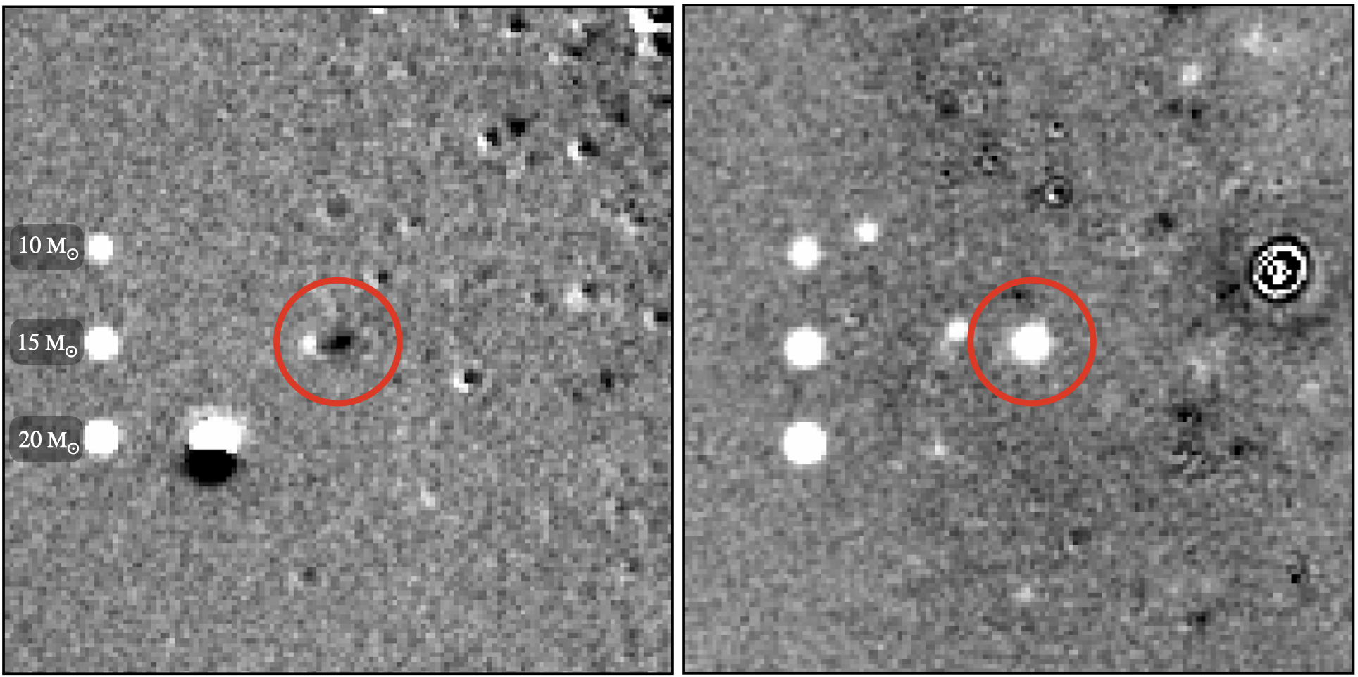
Figure 1: The average of the three most recent subtracted, LBT R band images of SN 2013ej (left) and SN 2011dh (right) with the SN position indicated by the 3$\aas@@fstack{\prime\prime}$0 circle. The three sources arranged vertically to the left of each SN are the expected signals for 10 (top), 15 (middle), and 20 $M_{\odot}$ (bottom) progenitors. While the subtractions for SN 2013ej are not the cleanest, it is presently more luminous than its progenitor and fading.

SN	Type	Host	Distance	Distance	Galactic	Host	Host Extinction	Apparent R	Peak
			(Mpc)	Reference	$E(B-V)$	$E(B-V)_{host}$	Reference	Peak Mag	Reference
SN 1980K	IIL	NGC 6946	5.96	1	0.291	0.07	8	11.45	21
SN 1993J	IIb	M81	3.65	2	0.069	0.13	9	$10.47$	22
SN 2002hh	II-P	NGC 6946	5.96	1	0.290	1.63	10	$15.54$	23
SN 2003gd	II-P	NGC 628	8.59	4	0.060	$0.07\pm 0.06$	11	$13.63$	24
SN 2004dj	II-P	NGC 2403	3.56	5	0.035	$0.026\pm 0.002$	12	$11.51$	25
SN 2005cs	II-P	NGC 5194	8.30	6	0.031	$0.01$	13	14.36	26
SN 2009hd	IIL	NGC 3627	10.62	3	0.029	$1.19\pm 0.05$	14	15.75	27
SN 2011dh	IIb	NGC 5194	8.30	6	0.031	$0.04$	15	12.25	28
SN 2012fh	Ib/c	NGC 3344	6.90	7	0.028	$\simeq 0$	16	16.24	29
SN 2013am	II-P	NGC 3623	10.62	3	0.021	$0.55\pm 0.19$	17	15.59	30
SN 2013ej	IIL	NGC 628	8.59	4	0.060	$\simeq 0$	18	12.43	31
SN 2016cok	II-P	NGC 3627	10.62	3	0.029	$0.50\pm 0.02$	19	15.25	32
SN 2017eaw	II-P	NGC 6946	5.96	1	0.297	$0.11\pm 0.05$	20	12.44	31

Table 1: The Galactic extinction from Schlafly & Finkbeiner (2011), for an assumed foreground reddening law of $R_{V}=3.1$. The horizontal line separates SNe without pre-SN LBT data (top) from those with pre-explosion LBT data (bottom). The apparent peak magnitude for SN 1980K is the V band magnitude used for the dust echo analysis. References: (1) Karachentsev et al. (2000), (2) Gerke et al. (2011), (3) Kanbur et al. (2003), (4) Herrmann et al. (2008), (5) Willick et al. (1997), (6) Poznanski et al. (2009), (7) Verdes-Montenegro et al. (2000), (8) Sugerman et al. (2012), (9) Zsíros et al. (2022), (10) Meikle et al. (2002), (11) Hendry et al. (2005), (12) Guenther & Klose (2004), (13) Baron et al. (2007), (14) Elias-Rosa et al. (2011), (15) Ergon et al. (2014), (16) Margutti et al. (2012), (17) Zhang et al. (2014), (19) Valenti et al. (2014), (19) Kochanek et al. (2017b), (20) Buta & Keel (2019), (21) Barbon et al. (1982), (22) Richmond et al. (1994), (23) Tsvetkov et al. (2007), (24) Hendry et al. (2005), (25) Tsvetkov et al. (2008), (26) Pastorello et al. (2006), (27) Elias-Rosa et al. (2011), (28) Ergon et al. (2014), (29) Zheng et al. (2022), (30) Zhang et al. (2014), (31) Bose et al. (2015), (32) de Jaeger et al. (2019), (33) Buta & Keel (2019) .

2 Observations and Models

The data are obtained using the Large Binocular Camera (LBC, Giallongo et al. (2008)) on the LBT (Hill et al., 2006) in the U, B, V, and R bands with image subtraction done using ISIS (Alard & Lupton, 1999; Alard, 2000). The details of the data processing are given in Gerke et al. (2015), Adams et al. (2017b), and Neustadt et al. (2021). For SNe with observations obtained pre-event, we built the reference images using the best observations before the explosion. With these reference images, difference imaging photometry will yield a “negative" image of the progenitor as the SN fades completely.

Lower quality data points are flagged as those with seeing FWHM $>1\aas@@fstack{\prime\prime}5$ or an ISIS flux scaling factor $<0.8$. This scaling factor is the counts per unit flux compared to the reference image and thus is an estimate of the transparency for each epoch relative to a flux reference epoch. For the calibrations, we follow the same methods as Gerke et al. (2015), and Adams et al. (2017b). Stars in the reference images are matched to the Sloan Digital Sky Survey (SDSS, Ahn et al. 2012) and the corresponding ugriz AB magnitudes are transformed into UBVR Vega magnitudes following Jordi et al. (2006). Following Johnson et al. (2018a), we extract light curves for both the target and a grid of comparison points to characterize the local noise. An inner grid of four points is placed 7 pixels apart (${\sim}$1$\aas@@fstack{\prime\prime}$6 given the plate scale of 0$\aas@@fstack{\prime\prime}$23 pixel^-1). The outer grid is placed 15 pixels away or ${\sim}$3$\aas@@fstack{\prime\prime}$5. Figures 4-10 show the resulting difference image light curves grouped by SN type. The formal errors are shown but are generally small which is why we look at the comparison points. We compute band luminosities ($\nu L_{\nu}$) using the distances and extinctions in Table 1. The extinction corrections for SN 2002hh are enormous, nearly 10 magnitudes in the U band.

We fit the late time (meaning well into the nebular phase) light curves as a linear function in luminosity ($\nu L_{\nu}$ for each band),

$$L=L_{SN}+\beta_{SN}(t-t_{0})$$ (1)

with $t_{0}$ being the mean age of the points being fit so that there are no significant covariances between the two parameters $L_{SN}$ and $\beta_{SN}$. We do the same for the light curves of the comparison points. Tables 5 and 6 report $L_{SN}$ and $\beta_{SN}$ and their uncertainties for each of the SNe. From the comparison points we report the mean values $\langle L_{i}\rangle$ and $\langle\beta_{i}\rangle$ and the dispersion of the values $\sigma_{L}$ and $\sigma_{\beta}$. Cases like SN 2009hd where there is significant dispersion in the comparison sample are a strong indication that the values are dominated by systematics. As mentioned earlier, the image subtractions for SN 2009hd are not very clean, driving the measured values and the large scatter. We do not consider SN 2009hd further.

The image subtraction light curves do not include the flux of the source in the reference image. For the SN with pre-SN images, this corresponds to the flux of the progenitor star. For the other SN, it is simply the mean flux of the SN over the images used to construct the reference image. We used aperture photometry to estimate the flux in the reference image, and the resulting luminosity is also reported in Tables 5 and 6. Particularly in the case of the progenitor stars, crowding generally makes the flux unmeasurable, so the luminosity estimates are dominated by systematic uncertainties. This is the reason why we focus on the subtracted light curves, which are little affected by crowding, separate from the reference flux.

Table 2 summarizes the cases where there are HST observations that can be used to explore this normalization. These are either pre-explosion observations for the SN with pre-SN LBT observations, or late time observations that (nearly) overlap the LBT observations. We converted the HST magnitudes to band luminosities using the HST zero points and the distances and extinctions from Table 1, and these band luminosities are reported in Table 2. We are interested in basic normalizations, not modest filter differences, so we simply view the HST filter as representing the closest equivalent LBT filter (so, for example, V=F555W=F606W). While we are frequently worried about line emission, we do not think these details represent a serious concern given the wavelength ranges of the filters.

To characterize the late time photometric evolution of each of the SNe, we must consider the expected properties of the progenitor star and then the 5 possible sources of late time luminosity: radioactive decay, CSM interactions, dust echoes, neutron star spin down, and shock heated companions.

2.1 Progenitor Stars

While we consider a broader range of supernovae, the most interesting cases are the 6 where we can construct a reference image from pre-supernova data. For a reference image built from pre-SN images, we will be left with an “inverse image" of the progenitor once the SN has completely faded. SN 2011dh, shown in Fig. 1, is the one case out of these 6 where this appears to have occurred. We model its spectral energy distribution (SED) following the procedures of Adams & Kochanek (2015) using DUSTY (Ivezic & Elitzur, 1997; Ivezic et al., 1999; Elitzur & Ivezić, 2001) so that we can consider self-obscuration and Solar metallicity stellar atmosphere models (Castelli & Kurucz, 2003).

Figure 2 shows the expected UBVR band luminosities along with the bolometric luminosity as a function of the initial progenitor mass $M_{ZAMS}$ for the Solar metallicity PARSEC (Bressan et al., 2012; Marigo et al., 2013) isochrones. The Groh et al. (2013) progenitor luminosities are similar. The bolometric luminosity is roughly a power law in mass, with

$$\log L_{prog}\simeq 4.8+1.5\log(M/10M_{\odot}).$$ (2)

In the PARSEC models, the stars are RSGs for $M_{ZAMS}\lesssim 30M_{\odot}$ so the stars are faintest in the U band and brightest in the R band. The mass loss monotonically increases with mass, so there is a small transition region where the temperatures lead to the emission peaking in the optical, and then the stars are very hot, heavily stripped stars that are brightest in the U band and faintest in the R band. With binary interactions, the temperatures at a given mass can be very different, but the bolometric luminosity is still basically set by the helium core mass.

Figure 2: UBVR and bolometric luminosities of SN progenitors at death for the Solar metallicity PARSEC isochrones. The horizontal dashed line is the estimated luminosity of the progenitor of SN 2011dh.

2.2 Radioactive Decay

All SN will show emission due to radioactive decay, initially dominated by ⁵⁶Ni, then ⁵⁷Co and finally ⁴⁴Ti (e.g., Seitenzahl et al. 2014). A typical Type IIP SN synthesizes $M_{\text{Ni}}<0.1M_{\odot}$ (Sukhbold et al., 2016). The ⁵⁶Ni luminosity is

$$L(t)=1.45\times 10^{43}\bigg{(}\frac{M_{\text{Ni}}}{M_{\odot}}\bigg{)}e^{-t/\tau_{0}}\text{erg s}^{-1}$$ (3)

where $\tau_{0}=111.3$ (Nadyozhin, 1994). The time required for the luminosity to fade below a threshold luminosity, L, is

$$t_{fade}=3.2+0.7\log\Bigg{[}\bigg{(}\frac{10^{4}L_{\odot}}{L}\bigg{)}\bigg{(}\frac{M_{\text{Ni}}}{0.1M_{\odot}}\bigg{)}\Bigg{]}\text{ yr}.$$ (4)

This neglects $\gamma$-ray escape, which would lead to a more rapid decline in luminosity (Seitenzahl et al., 2014). For the typical Ni masses produced in a Type II-P SN of $M_{\text{Ni}}<0.1M_{\odot}$ (Sukhbold et al., 2016), the time scale for the radioactive decay luminosity to be less than the progenitor luminosity is roughly 3-4 years. For example, SN 1987A had a luminosity of $\sim 30000L_{\odot}$ ($\sim 3000L_{\odot}$) after 1000 (2000) days and $M_{\text{Ni}}=0.071\pm 0.003M_{\odot}$ (Seitenzahl et al., 2014). We will estimate the required $M_{\text{Ni}}$ masses empirically by scaling the SN 1987A V-band light curve from Seitenzahl et al. (2014) to the LBT data. While we phrase the result in terms of $M_{\text{Ni}}$, the emission at these late times should be from ⁴⁴Ti.

2.3 Circumstellar Medium (CSM) Shock Interactions

Following the SN, the expanding ejecta will shock heat any pre-existing circumstellar medium (CSM), exciting optical emission lines which contribute to the late time luminosity (e.g., Chevalier 1982a). For a spherically symmetric $\rho\propto 1/r^{2}$ pre-SN wind, the optical shock luminosity is

$$L_{s}\simeq\epsilon\frac{1}{2}\dot{M}\frac{v_{s}^{3}}{v_{w}}$$

$$\simeq 53000\left({\frac{\epsilon}{0.1}}\right)\Bigg{(}\frac{\dot{M}}{10^{-6}M_{\odot}\text{yr}^{-1}}\Bigg{)}\Bigg{(}\frac{v_{s}}{4000\text{km~{}s}^{-1}}\Bigg{)}^{3}\Bigg{(}\frac{10\text{km~{}s}^{-1}}{v_{w}}\Bigg{)}L_{\odot}$$ (5)

where $v_{s}$ is the shock speed, $\dot{M}$ is the wind mass loss, $v_{w}$ is the wind speed and $\epsilon$ is the fraction of the luminosity emitted in the optical. For luminosities comparable to the progenitor or lower, the inertia of the swept up CSM is only modestly slowing the shock, so the ability of the shock to support late time emission is largely controlled by the efficiency $\epsilon$ of converting the shock energy into optical emission. The physics of $\epsilon$ is very complex, since it depends on the balance of emission mechanisms and the radiative efficiency. For our standard results we will simply match the R-band luminosity ($\nu L_{\nu}$) assuming $\epsilon=0.1$, $v_{s}=4000$ km/s and $v_{w}=10$ km/s. We chose $\epsilon$ and $v_{s}$ to match Chandra et al. (2022) but use $v_{w}=10$ km/s (instead of 45 km/s) to match the assumption of the RSG mass loss models we consider later as well as most $\dot{M}$ estimates from X-ray and radio studies. We focus on the R band light curve since it contains the strong H$\alpha$ emission line. In our sample, CSM interactions have been invoked for SN 1993J (e.g., Suzuki et al. 1993, Leising et al. 1994, Suzuki & Nomoto 1995, Fransson et al. 1996), SN 2002hh (e.g., Chevalier et al. 2006), SN 2004dj (e.g., Chevalier et al. 2006, Chakraborti et al. 2012), SN 2011dh (e.g., Soderberg et al. 2012, Maeda et al. 2014), SN 2013ej (e.g., Mauerhan et al. 2017), and SN 2017eaw (e.g. Weil et al. 2020). These $\dot{M}$ estimates are given in Table 4.

As illustrated by the theoretical models of Dessart & Hillier (2022) or the late time spectra of SN 1993J from Matheson et al. (2000a), the optical CSM emission is dominated by emission lines, so the color of the emission should distinguish it from continuum emission like dust echoes and shock heated secondaries. Fig. 3 shows the colors of their model with 1 M_⊙ of ejecta travelling at $10^{4}$km s^-1, which provides a reasonable match to the Matheson et al. (2000a) spectra of SN 1993J $976$ days after peak, as compared to the Solar metallicity PARSEC (Bressan et al. 2012, Marigo et al. 2013) isochrones with ages of $10^{6.6}$ to $10^{7.2}$ years. We also show the colors of the emission from the shock heated ring in SN 1987A using the fluxes from Larsson et al. (2019) over the time period from 3200 to 11000 days after peak. In SN 1987A, the emission peaks nearly 22 years after the explosion, with B, V, R luminosities of roughly $\sim 60L_{\odot}$, $\sim 10L_{\odot}$ and $\sim 160L_{\odot}$, respectively, that are orders of magnitude less than the luminosity scales of the progenitor stars shown in Fig. 2. This particular color combination, B$-$V and V$-$R, appears to be a good combination for identifying systems dominated by line emission because the R band contains the strong H$\alpha$ emission, and the B band contains strong O[III] emission while the H$\beta$/O[III] emission lines in the V band are generally weaker. This should give CSM emission blue B$-$V colors and red V$-$R colors which are difficult for less line dominated spectra to mimic, as seen in Fig. 3.

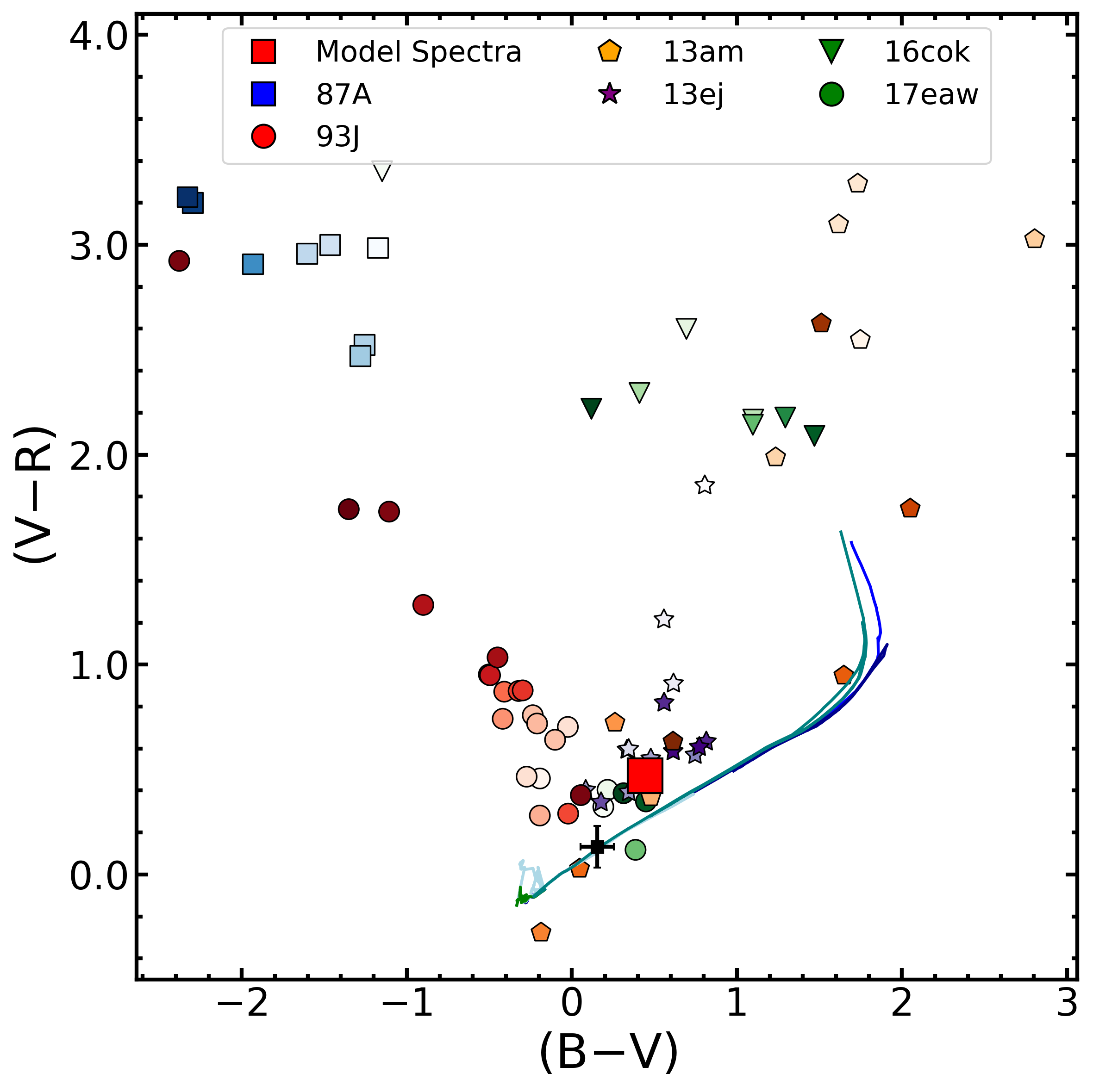
Figure 3: Colors of the late time emission compared to the model CSM interaction spectra (red square) from Dessart & Hillier (2022) and SN 1987A (blue squares) from Larsson et al. (2019). Darker colors represent later time epochs from the peak. The solid lines are Solar metallicity PARSEC isochrones with ages from $\log_{10}$(Age) = 6.6 to 7.2. The black cross is the mean, near-peak, extinction corrected colors for 5 of the SNe. The size of the cross is for visibility - the scatter in the colors is less than the size of the symbol.

2.4 Dust Echos

When light from a SN encounters interstellar dust, it can be scattered to reach us with a light travel time delay. The detailed properties of light echos are dependent on multiple parameters such as dust location, geometry, and scattering optical depth (e.g., Chevalier 1986, Sugerman 2003, Liu et al. 2003, Rest et al. 2005, Rest et al. 2011). We can roughly characterize the luminosity as

$$L=\frac{E_{rad}\tau_{dust}}{t_{now}}$$ (6)

where $E_{rad}$ is the energy radiated in the photometric band, $t_{now}$ is the time elapsed since peak, and $\tau_{dust}$ is the fraction of $E_{rad}$ that is scattered to the observer. This model essentially assumes that the dust is in a shell a distance $ct_{now}$ from the SN that is absorbing fraction $\tau$ of the radiated energy with light travel times then spreading the observed emission over time $t_{now}$. Dust echoes have (roughly) the emission weighted mean spectrum of the SN, weighted by the smoothly varying, direction-dependent scattering opacity of the dust. For our sample, dust echoes are reported for SN 1980K (Sugerman et al. 2012, Bevan et al. 2017), SN 1993J (Sugerman & Crotts 2002, Liu et al. 2003), SN 2002hh (Welch et al. 2007, Andrews et al. 2015), SN 2003gd (Sugerman, 2005). For these SNe, the observed light echos are generally bluer than the color of the SN near peak.

We again make the estimates using the R band data, in this case because it generally has smaller uncertainties. The data are collected using the LBC/Red camera for the R-band while cycling through UBV on the LBC/Blue camera, leading to shorter exposure times for the other filters. We estimate the the total radiated energy $E_{rad}$ using the Morozova et al. (2015) light curve models normalized to the peak R-band peak luminosity given in Table 1. We then simply estimate $\tau_{dust}$ using Eqn. 6. The basic physics of echoes requires the $1/t_{now}$ decay unless the effective optical depth is increasing with distance from the SN. Fig. 3 shows the mean, near-peak colors of SN 1993J, 2013am, 2013ej, 2016cok, and 2017eaw after correcting for extinction. The scatter in the colors is smaller than the symbol. We would expect dust echoes to be modestly bluer than these colors.

2.5 Engine Driven Emissions

Another possibility for driving late time emissions is energy injection from a pulsar. If we assume dipole spin down, the luminosity is

$$L=\frac{4\pi^{2}I}{P^{2}t_{s}}=330000I_{45}P_{10}^{-2}t_{4}^{-1}L{}_{\odot}$$ (7)

for moment of inertia $I=10^{45}$ g cm², spin period $P=10P_{10}$ msec, and spin down time $t_{s}=10^{4}t_{4}$ years. The spin down time is related to the magnetic field $B=10^{12}B_{12}$ gauss by

$$t_{s}=P\dot{P}^{-1}=13000B_{12}^{-2}P_{10}^{2}~{}\hbox{year}.$$ (8)

For the Crab pulsar ($P=0.033$ s, $t_{s}=2600$ years), $L=1.1\times 10^{5}L_{\odot}$. However, essentially none of this energy is converted into visible radiation at late times. For the optical magnitudes of the Crab from Sandberg & Sollerman (2009), a distance of $2$ kpc (Kaplan et al., 2008) and an extinction of $E(B-V)\simeq 0.4$ mag (Green et al., 2019), the UBVR luminosities of the Crab are $<10L_{\odot}$. Magnetar models (e.g., Kasen & Bildsten 2010), assume that the spin down energy is fully thermalized and that the amount radiated is regulated by the balance between the expansion and diffusion times. We are considering the emission at late times in the nebular phase, where the prediction of these models is that the luminous emissions are strongly suppressed and we would expect properties more like the Crab. For this reason, we do not consider engine driven emissions further.

2.6 Binary Companion Ejecta Interaction

When the shock from a SN hits a binary companion, it heats and inflates its envelope, which leads to a period of enhanced luminosity (Wheeler et al. 1975, Fryxell & Arnett 1981, Marietta et al. 2000, Podsiadlowski 2003, Meng et al. 2007, Hirai et al. 2014, Hirai et al. 2018, Ogata et al. 2021). We use the numerically calibrated analytic model of Ogata et al. (2021) to constrain the companion mass ($M_{c}$), and the ratio of its radius to the orbital separation ($R_{c}/a$). The total energy injected into the companion from the outburst is

$$E_{heat}=pE_{expl}\tilde{\Omega}$$ (9)

where $p\simeq 8-10\%$ is the energy injection efficiency, $E_{expl}=10^{51}$erg is the explosion energy, and

$$\tilde{\Omega}=\frac{1}{2}\Bigg{[}1-\sqrt{1-\Bigg{(}\frac{R_{c}}{a}\Bigg{)}^{2}}\Bigg{]}$$ (10)

is the fractional solid angle subtended by the companion. The maximum luminosity of the companion is

$$L_{max}=\frac{4\pi GM_{c}c}{\kappa_{fit}}$$ (11)

where $\kappa_{fit}$ is a fitting function from Ogata et al. (2021) for the average opacity at the bottom of the companion’s convective layer, $G$ is the gravitational constant, $c$ is the speed of light, and $M_{c}$ is the companion mass. Thus, the maximum luminosity is determined by the companion mass. The timescale over which the companion maintains this luminosity is,

$$\tau_{infl}=\alpha\frac{E_{heat}}{L_{max}}$$ (12)

where $\alpha=0.18$. Since significant heating of a main sequence (MS) binary companion requires an orbit smaller than the RSG progenitors of Type II SNe, we consider this case only for the Type Ibc SN 2012fh.

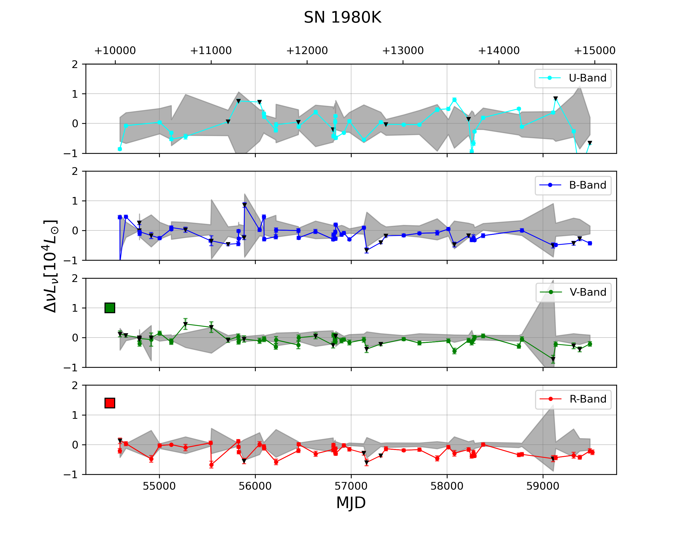
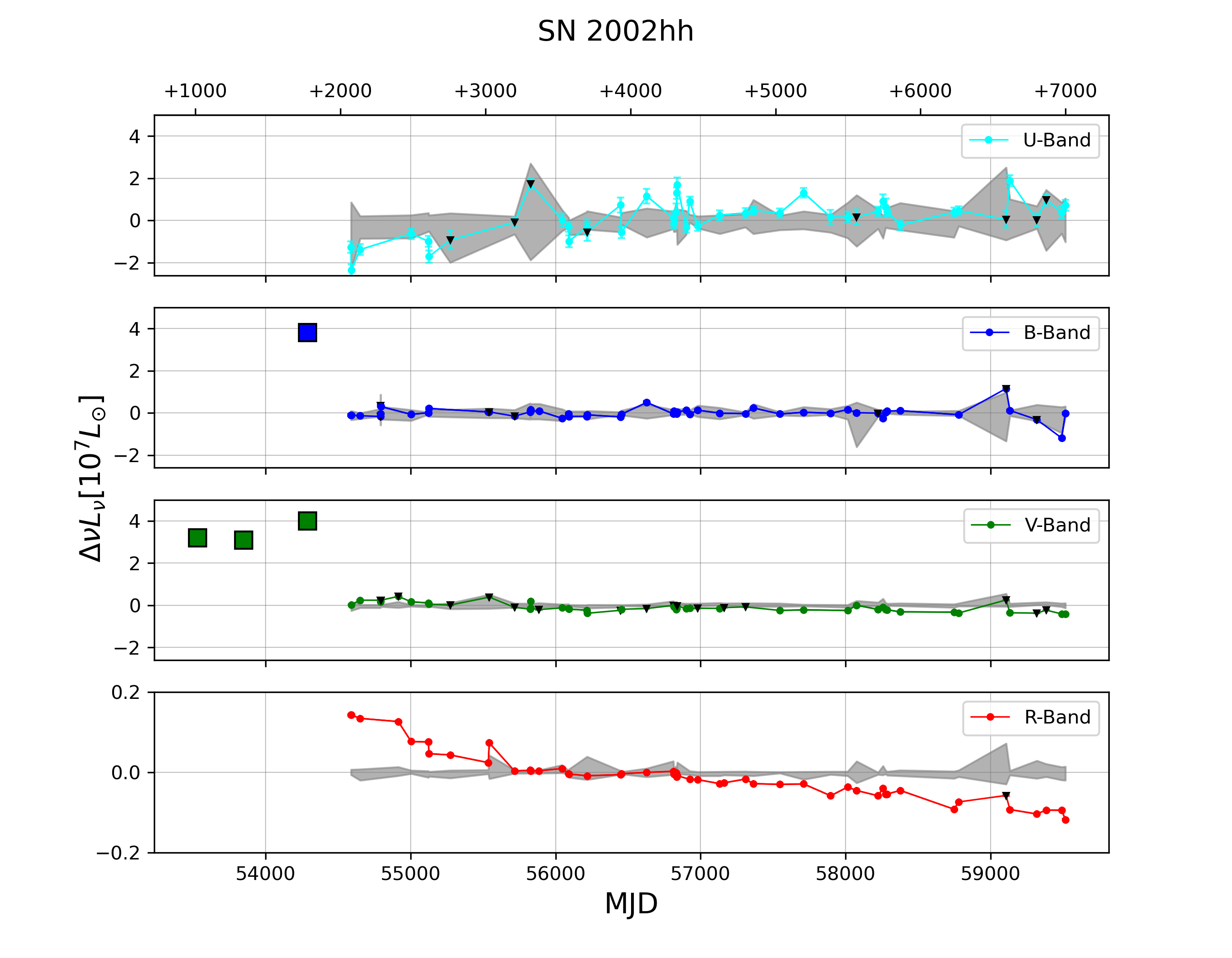
Figure 4: LBT UBVR difference imaging light curves for the Type IIP/L SNe with days after peak shown at the top and black triangles for poorer quality epochs as defined in § 2. The gray region is the 1$\sigma$ scatter about the mean of the 11 comparison light curves. For SNe with pre-SN images, the vertical dashed line is the date of peak. The large squares are the HST photometry from Table 2 where available. The star symbol denotes the epoch at which the linear fits provided in Tables 5 and 6 begin. For SNe which exploded prior to the LBT survey, the entire light curve is fit. Except for 2011dh, 2013am, 2016cok, and 2017eaw where the luminosity is in units of $10^{5}L_{\odot}$, 2009hd in units $10^{6}L_{\odot}$, and 2002hh in units $10^{7}L_{\odot}$, the luminosity is in units of $10^{4}L_{\odot}$. The range shown varies between the SNe for clarity. The luminosity is relative to the luminosity in the reference image, which for SNe with pre-explosion imaging is the luminosity of the progenitor.

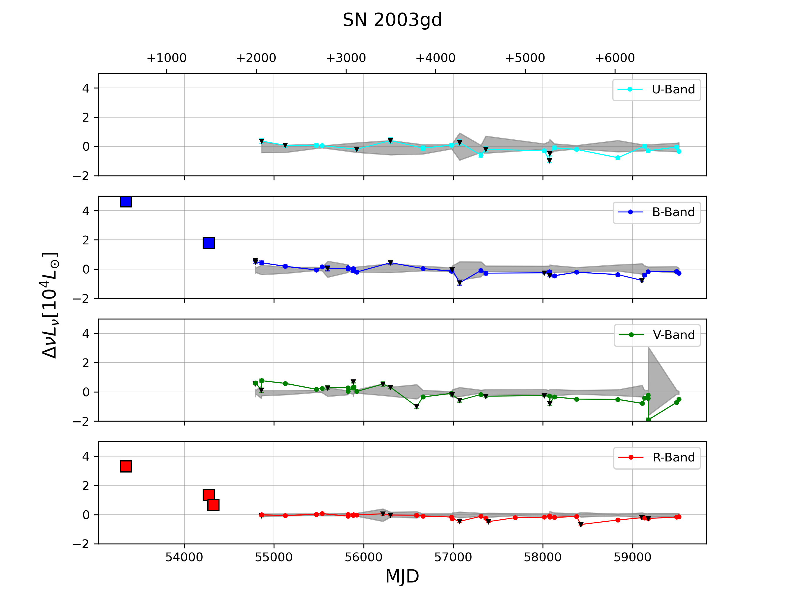
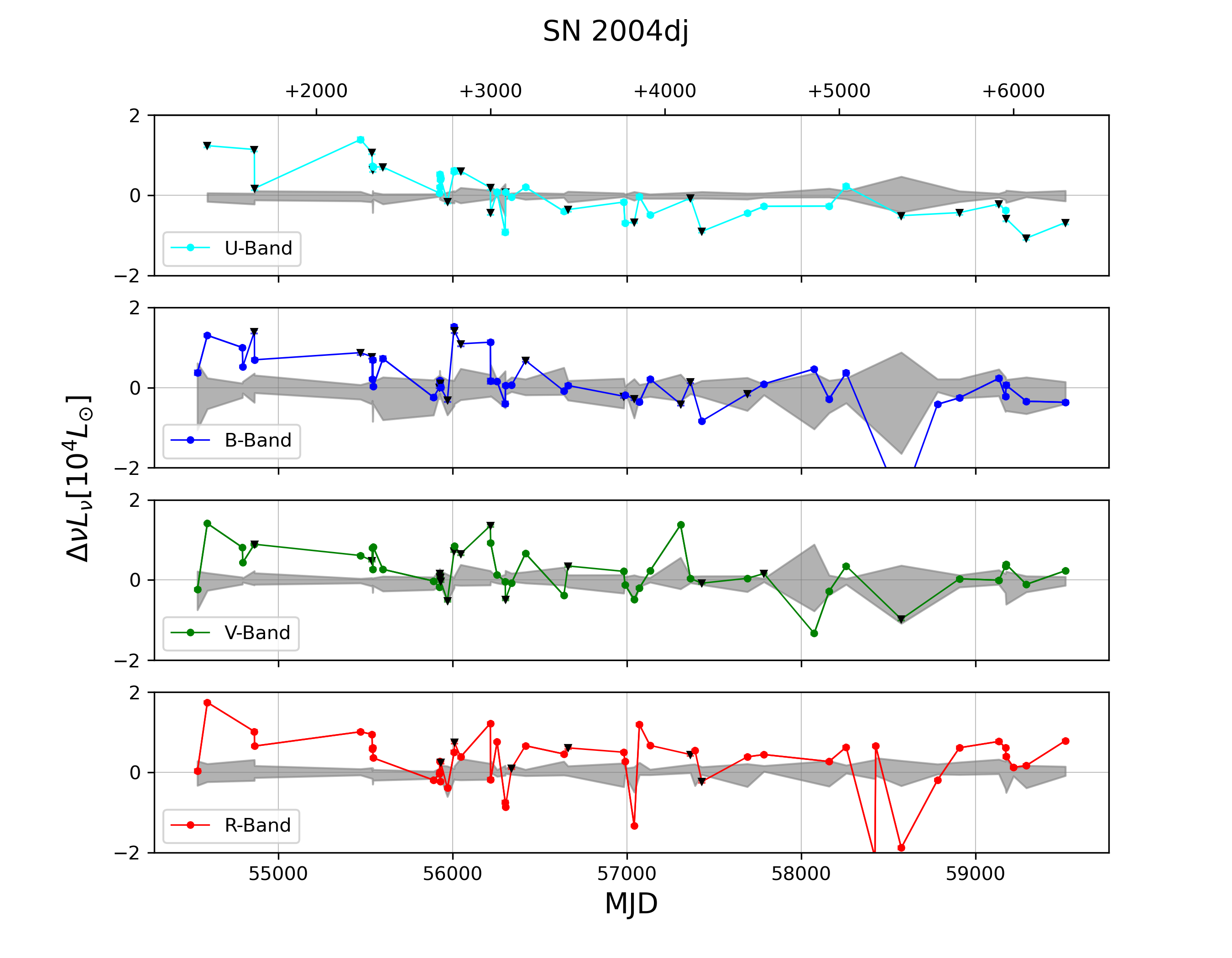
Figure 5: Type IIP/L (cont.)

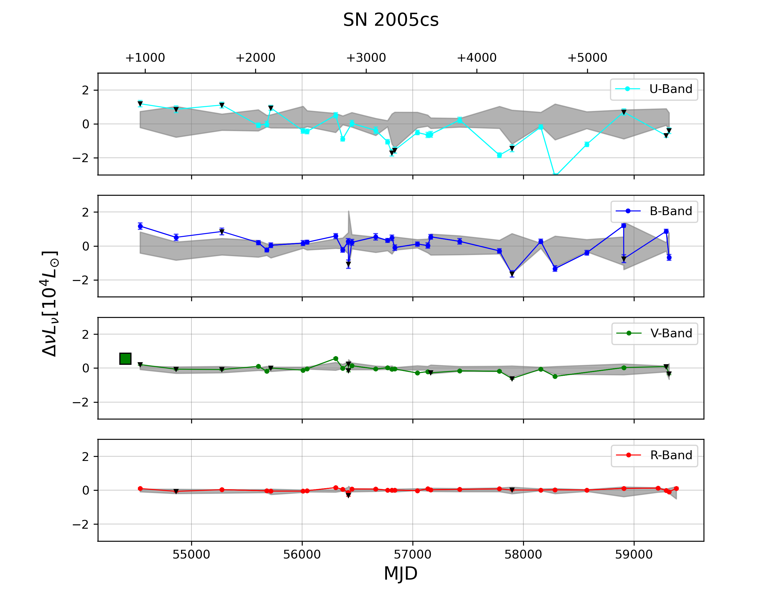
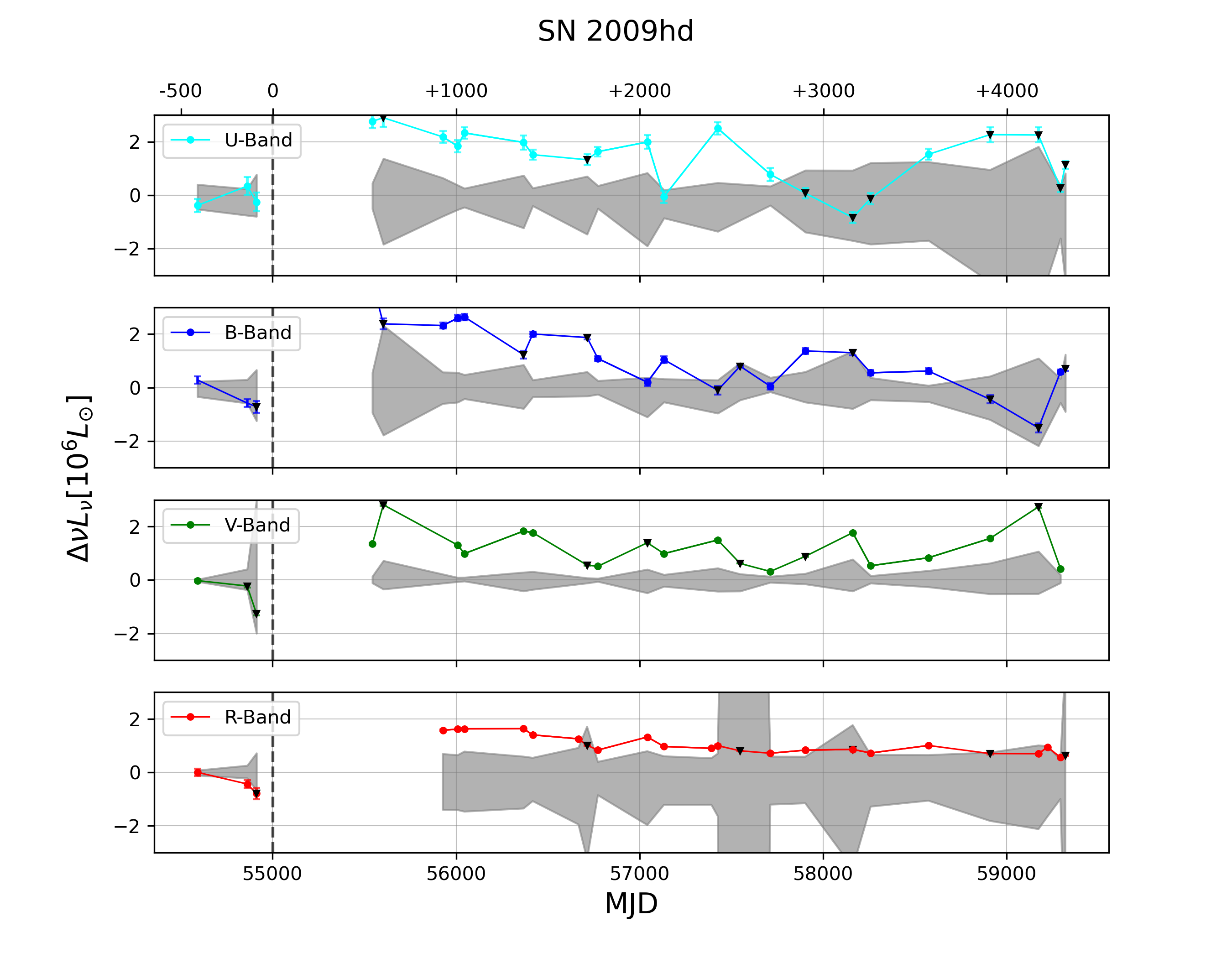
Figure 6: Type IIP/L (cont.)

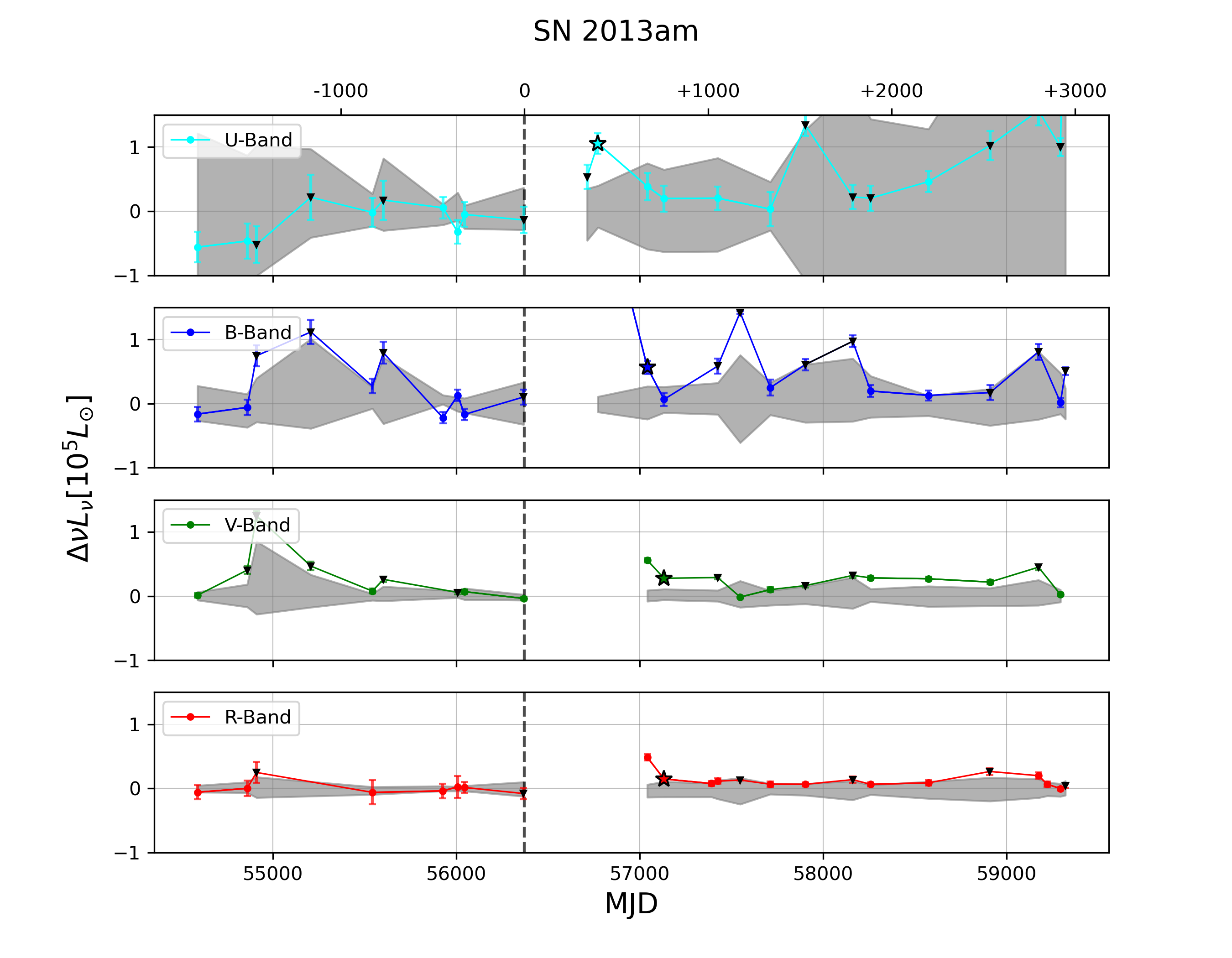
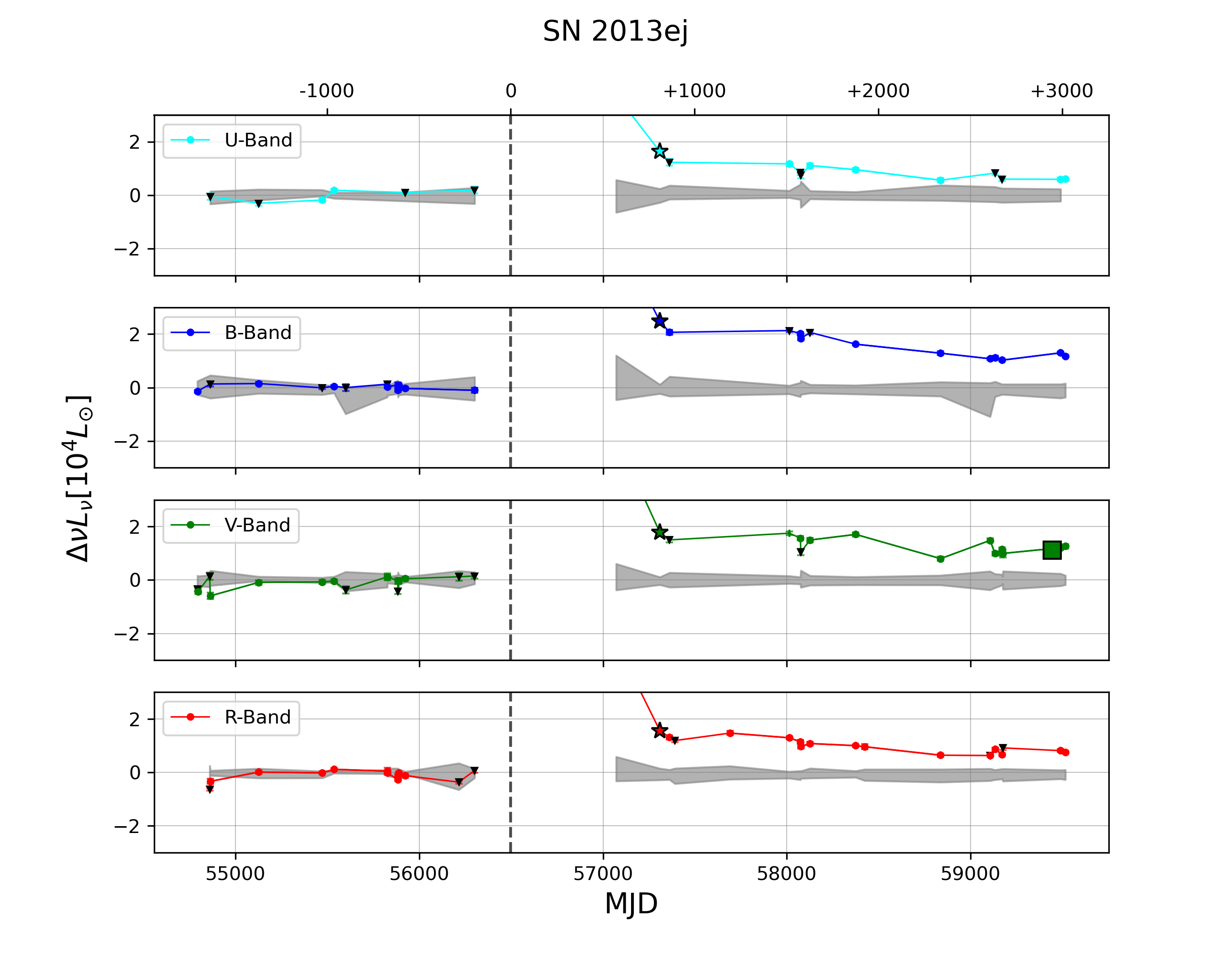
Figure 7: Type IIP/L (cont.)

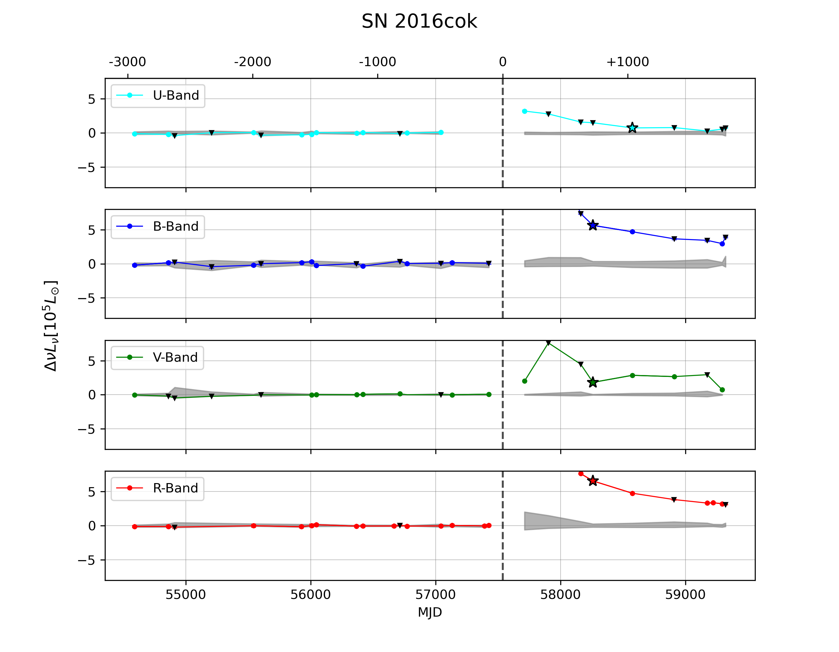
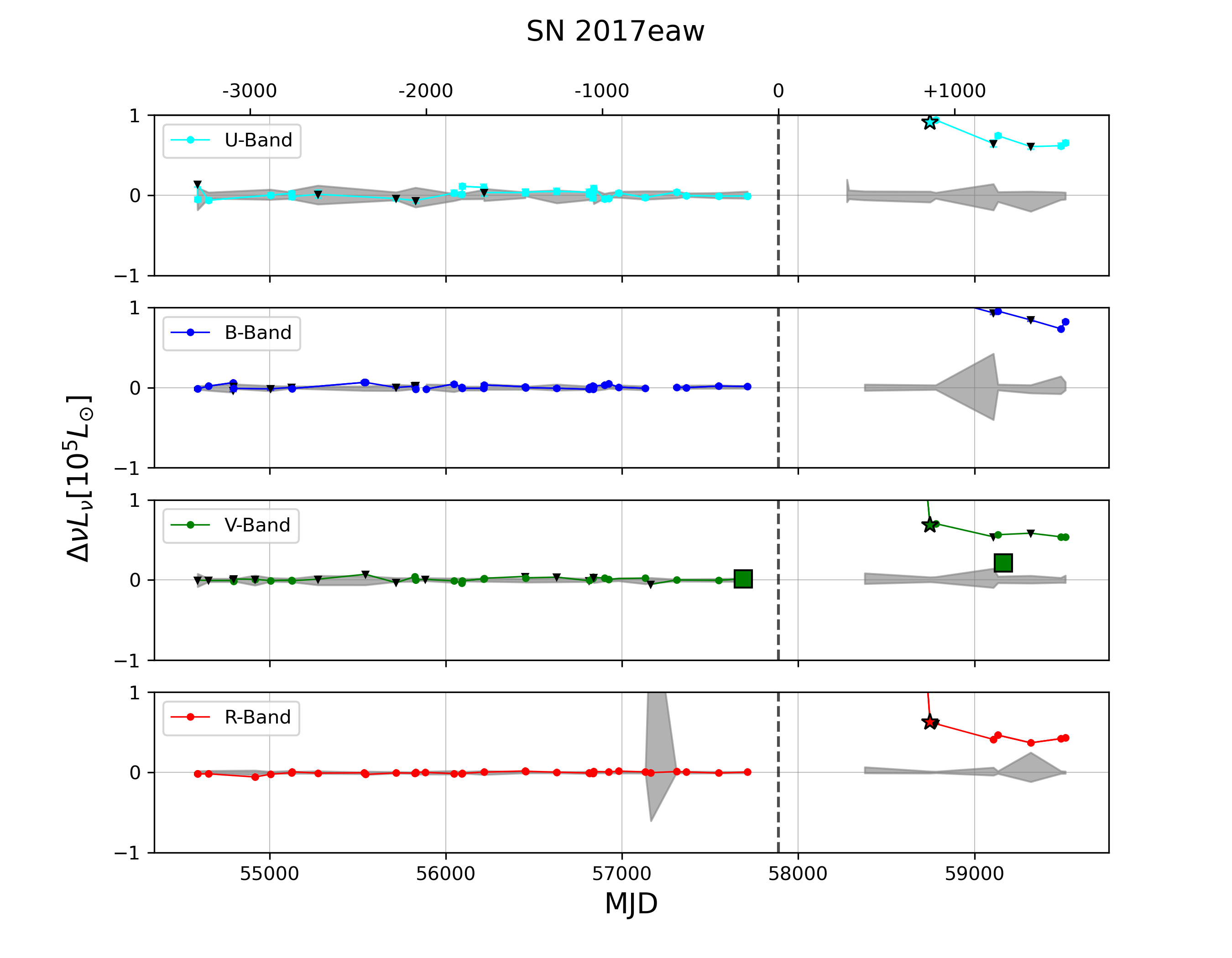
Figure 8: Type IIP/L (cont.)

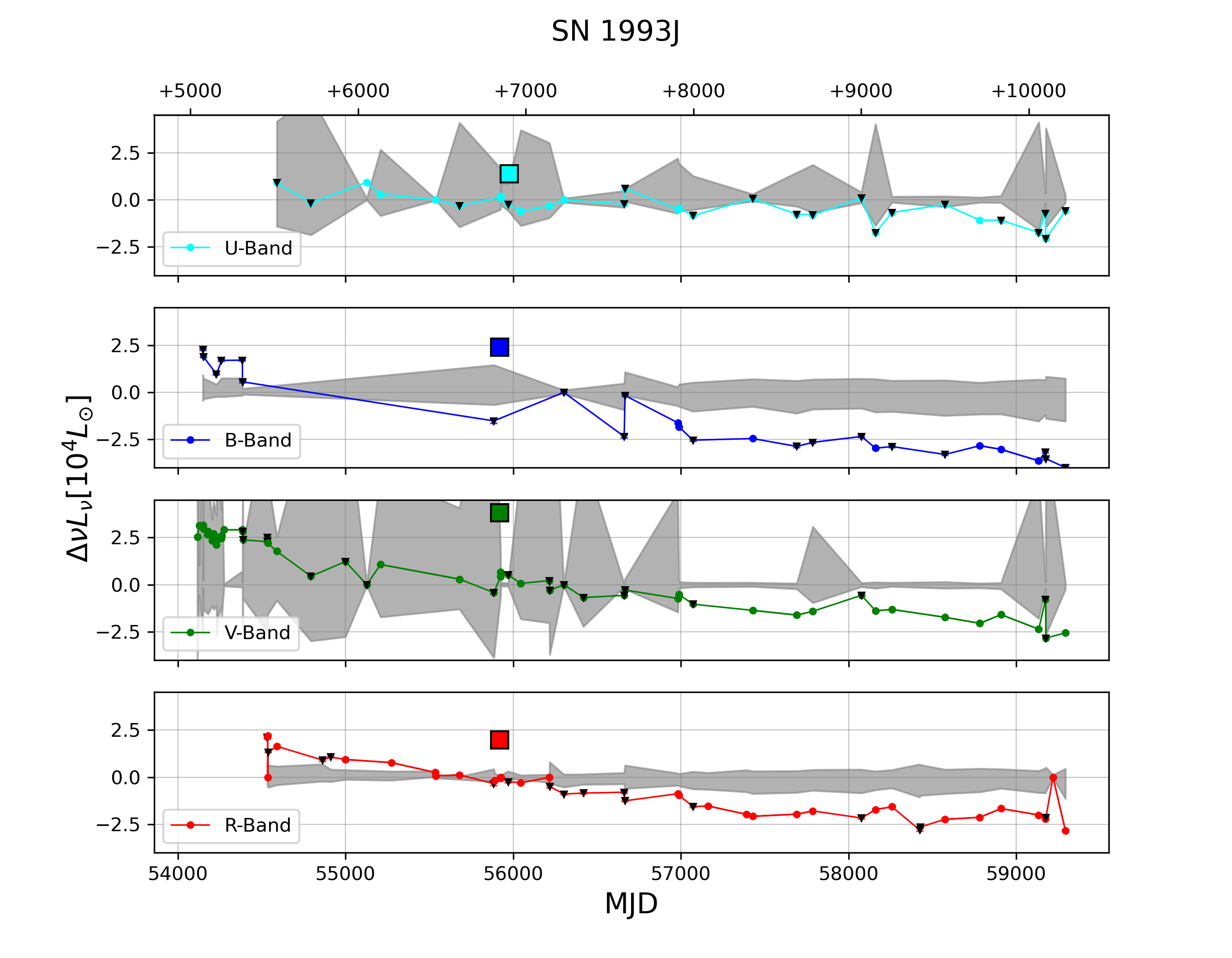
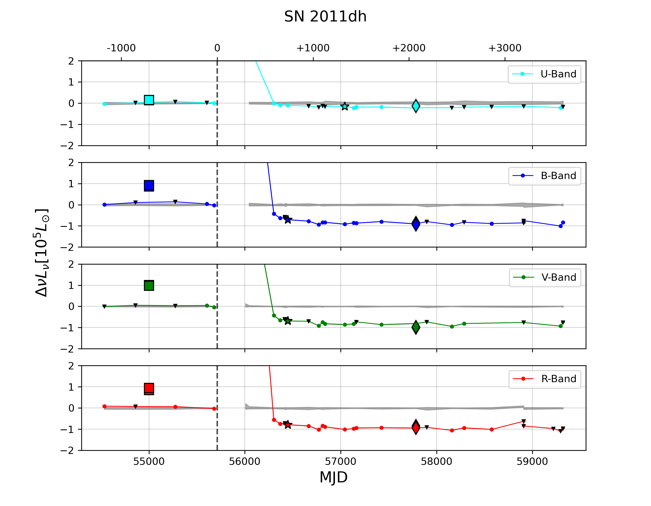
Figure 9: LBT UBVR difference imaging light curves for the Type IIb SNe. The large squares are the HST photometry from Table 2 where available. For SN 2011dh the pre-SN HST observations occurred at an earlier epoch and are shifted to the date shown. For SN 2011dh, the diamonds are the inverse of HST photometry at the epoch we perform the SED fit as described in § 3.1.

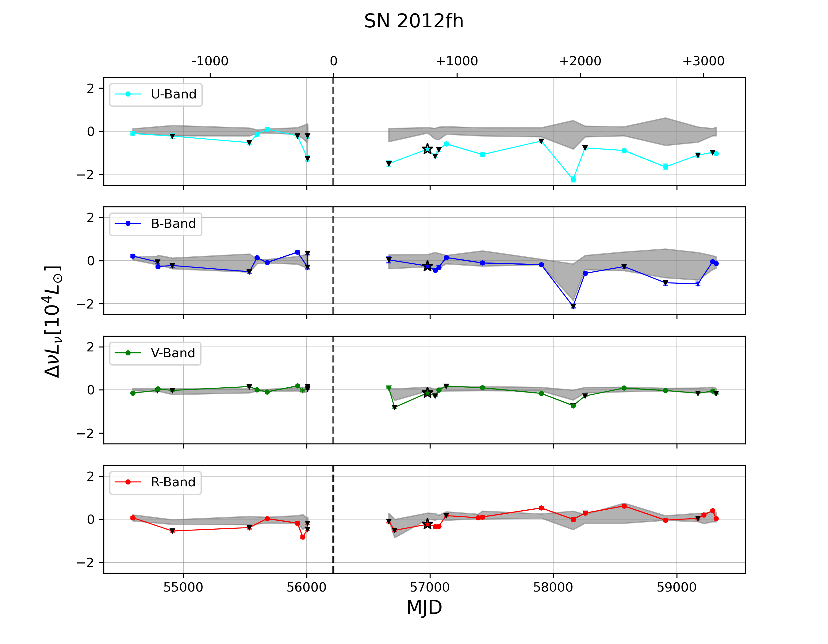
Figure 10: LBT UBVR difference imaging light curves for the Type Ib/c SN

3 Discussion

Table 1 summarizes the SN we consider, and the Appendix A has notes on the individual sources. After dropping SN 2009hd, there are 12 sources in total; 9 IIL/P, 2 IIb, and 1 Ib/c, of which 4, 1, and 1 have pre-SN LBT observations. Figures 4–10 show the LBT light curves of the SN grouped by type and with the epoch of explosion marked if it occurred after the start of the LBT project. Tables 5 and 6 give the results of the linear fits to the late time light curves of each SNe and its grid of comparison points where the fits extend from the epoch marked in the figure through the end of the light curve. We include fits for SN 2009hd even though we will not discuss it further.

The luminosities of the SNe in these light curves are all relative to the luminosity of the source in the reference image. For the SNe with pre-SN LBT data, the observed light curve is thus any present day emission minus the luminosity of the progenitor. For the SN with only late time LBT data, it is the present day emission minus the mean luminosity of the SN is the reference image flux. The aperture photometry luminosity of the SNe on the reference image is reported in Tables 5 and 6, but they should be generally regarded as limits due to the effects of crowding. Figures 4–10 include the HST luminosities from Table 2. The offset between the differential luminosity light curve and the HST luminosity is the luminosity in the reference image. Where the HST data is available, the actual light curve is simply the differential light curve shifted upwards in luminosity to pass through the HST data. What we see in general is that the necessary shifts are on the same scale as the changes in luminosity. The exception is SN 1980K, where the HST luminosity is roughly an order of magnitude larger. SN 1980K is also the only case where we can clearly see the SN in the LBT data at these late times.

For our standard analyses we use the image subtraction light curve if the linear fit estimate of the luminosity of the last epoch is positive. If the linear fit estimate of the luminosity of the last epoch is negative, we rescale the final luminosity to zero and use $L_{SN}^{\prime}=L_{SN}-\beta_{SN}(t_{last}-t_{0})$ where $t_{last}$ the time of the last epoch. All of these latter systems are SNe without pre-explosion LBT images with the exception of SN 2011dh. This still means that our estimates of the ⁵⁶Ni mass, wind $\dot{M}$, and dust optical depth $\tau$ will be underestimates, so we discuss the consequences of further increases in the luminosities due to the (remaining) uncorrected flux in the reference image. We will also provide estimates based on the slope $\beta_{SN}$. For radioactive decay we can make a direct estimate of the ⁵⁶Ni mass by matching the slope of the LBT light curve to that of SN 1987A. For the other two emission mechanisms we make a “standardized” estimate using the luminosity $\beta_{SN}\Delta t$, the drop in luminosity over $\Delta t=10$ years. It is standardized in the sense that the time baselines for the most recent SN are much shorter than the full time baseline of the LBT data.

Of the 9 Type IIP/L systems, 8 show continued late time emission, particularly in the V and R bands. One of the Type IIb SN, SN 1993J, shows continued fading. Only the Type IIP SN 2005cs, the Type IIb SN 2011dh and the Type Ibc SN 2012fh do not show significant evidence for continued emission. For the systems with pre-LBT images, all but SN 2011dh and possibly SN 2012fh have a present day luminosity in excess of the progenitor. In the next sections we first discuss the progenitor of SN 2011dh, and then the potential sources of the continued emission for the other systems.

Figure 11: Spectral energy distribution models for the LBT (solid squares) and HST (open triangles) photometry of the progenitor of SN 2011dh fitting the temperature, luminosity, and extinction. The solid curve fits all of the points, while the dashed curve does not include the U/F336W data in the fits.

SN	Date	Band	Luminosity	Ref.
	(MJD)		($10^{4}L_{\odot}$)
SN 2003gd	52511	V	$0.26$	1
SN 2005cs	53380	V	$<0.32$	2
SN 2017eaw	57687	V	0.16	3
SN 1980K	54484	V	$1.0$	4
	54484	R	$1.4$	4
SN 1993J	55976	U	$1.39$	5
	55919	B	$2.39$	5
	55919	V	$3.81$	5
	55919	R	$1.97$	5
SN 2002hh	53630	V	$3200$	6
	53848	V	3100	6
	54290	B	3800	6
	54290	V	4000	6
SN 2003gd	53347	B	4.63	7
	53347	R	3.30	7
	54272	B	1.79	8
	54272	R	1.35	8
	54323	R	0.64	6
SN 2005cs	54079	V	9.66	6
	54401	V	0.56	6
SN 2013ej	59445	V	$1.12$	9
SN 2017eaw	59164	V	$2.13$	9

Table 2: Existing HST photometry of six SNe in this sample, the horizontal line separates the pre-explosion observations from the post-explosion observations. References: (1) Smartt et al. (2004), (2) Li et al. (2006), (3) Van Dyk et al. (2019), (4) Sugerman et al. (2012), (5) Fox et al. (2014), (6) Otsuka et al. (2012), (7) Sugerman (2005), (8) Maund & Smartt (2009), (9) Van Dyk et al. (2022)

3.1 Progenitor Constraints

As noted earlier, only SN 2011dh, a Type IIb SNe in NGC 5194, shows the originally expected fading. The SN was fainter than the progenitor within $\sim 600$ days, as expected from a light curve dominated by radioactive decay. In a reverse time average of the subtracted light curves, we begin to see an upward trend at times earlier than +1400 days post explosion, so we adopt the reverse time average of the light curves after day +2000 as the estimate of the progenitor flux. The principal limitation on our photometry is the calibration because the depths of the LBT data and the SDSS survey are poorly matched (particularly since SDSS only catalogs stars around the periphery of the galaxy). A shallower LBT image is needed to improve the calibration. Nonetheless, the LBT magnitudes in Table 3 are very similar to those found by Van Dyk et al. (2011) and Maund et al. (2011) analyzing the same HST F336W, F435W, F555W, F658N, and F814W images, roughly corresponding to the U, B, V, R and I bands. That they are so similar despite the need for a better calibration of the LBT data is a demonstration that it should be straight forward to obtain very good photometry of SNe progenitors from the LBT data once they have faded. Fig. 11 provides an extinction corrected SED.

We fit the data assuming minimum photometric errors of 10%, a fixed distance of $7.1\pm 1.2$ Mpc to match Van Dyk et al. (2011) and Maund et al. (2011) and varying only the luminosity, temperature and foreground extinction, with an extinction prior of $E(B-V)=0.05\pm 0.05$ mag. This includes both the Galactic extinction and any contribution from the host. For the LBT data the best fit has $\chi^{2}=21.0$ for two degrees of freedom, with $L_{*}=10^{5.00\pm 0.04}L_{\odot}$, $T_{*}=5294\pm 154$ K and $E(B-V)=0.02\pm 0.02$ mag. The poor fit is driven by an inability to find a model which is roughly flat in $\nu L_{\nu}$ for the B, V and R bands and then drops rapidly enough to fit the U band.

We did not fit the HST narrow band H$\alpha$ data (F658N), and for the Van Dyk et al. (2011) photometry the best fit has $\chi^{2}=8.2$ again for two degrees of freedom with $L_{*}=10^{4.98\pm 0.04}L_{\odot}$, $T_{*}=6312\pm 357$ K and $E(B-V)=0.10\pm 0.04$ mag. In their analysis, Van Dyk et al. (2011) adopted a temperature of $T_{*}=6000$ K and a luminosity of $L=10^{4.99}L_{\odot}$ and a fixed (Galactic) extinction of $E(B-V)=0.04$ mag. Finally, for the Maund et al. (2011) values we find $\chi^{2}=15.2$, $L_{*}=10^{5.00\pm 0.03}L_{\odot}$, $T_{*}=6317\pm 353$ K and $E(B-V)=0.12\pm 0.02$mag. Maund et al. (2011) found $L_{*}=10^{4.92\pm 0.20}L_{\odot}$ and $T_{*}=6000\pm 280$ K. Both of the HST fits also struggle with the rapid drop down to the F336W point, but the impact on the $\chi^{2}$ is smaller because of the larger uncertainty for HST F336W compared to the LBT U band. Using circumstellar dust instead of foreground extinction did not solve the problem of the poor fits to these data.

If we combine the LBT and Maund et al. (2011) data (again excluding the narrow band filter) we get $\chi^{2}=39.6$ for 7 degrees of freedom, $L_{*}=10^{4.97\pm 0.04}L_{\odot}$, $T_{*}=5601\pm 226$ K and $E(B-V)=0.04\pm 0.04$. If we drop the the U/F336W points, we find $\chi^{2}=2.1$ for 5 degrees of freedom with $L_{*}=10^{4.99\pm 0.05}L_{\odot}$, $T_{*}=6629\pm 324$ K and $E(B-V)=0.08\pm 0.04$ mag. Fig. 11 shows these combined models. For the adopted distance estimate, there is an additional uncertainty in the luminosity of $0.15$ dex from the uncertainties in the distance. This is likely already included in the Maund et al. (2011) luminosity uncertainty. All of these models agree on a progenitor luminosity very close to $10^{5}L_{\odot}$ and Fig. 2 shows how these luminosity estimates compare to the progenitor models. The close match to the HST data emphasizes the point in Fig 1 that faded progenitors should generally be trivially visible in the LBT data.

Maund (2019) argues for a late-time emission plateau at 2000-2500 days of roughly $10^{4}L_{\odot}$ fading by approximately $(-330\pm 110)L_{\odot}$/year, and argues for a dust echo since there are no indications of the presence of emission lines in their narrowband images. Such a low level contribution would have little effect on this analysis since the estimated progenitor luminosity is an order of magnitude higher. Formally, we find somewhat steeper decay rates in Table 6.

Band	LBT	Van Dyk	Maund
	[mag]	[mag]	[mag]
U	$23.18\pm 0.07$	$23.434\pm 0.339$	$23.39\pm 0.25$
B	$22.30\pm 0.02$	$22.451\pm 0.005$	$22.36\pm 0.02$
V	$21.66\pm 0.09$	$21.864\pm 0.006$	$21.83\pm 0.04$
R	$21.42\pm 0.04$	$21.392\pm 0.021$	$21.28\pm 0.04$
I		$21.216\pm 0.005$	$21.20\pm 0.03$

Table 3: Photometry of the progenitor of SN 2011dh. The Van Dyk et al. (2011) and Maund et al. (2011) magnitudes are the HST F336W, F435W, F555W, F658N and F814W filters.

	56Ni Mass			Mass Loss Rate		Scattering Optical Depth		Other $\dot{M}$ Estimates
	[M⊙]			[$\log_{10}(M_{\odot}\text{yr}^{-1})$]		[$\log_{10}(\tau)$]		[$\log_{10}(M_{\odot}\text{yr}^{-1})$]
SN	$10^{3}L_{\odot}$	LSN	$\beta_{SN}$	LSN	$\beta_{SN}\Delta t$	LSN	$\beta_{SN}\Delta t$	$\dot{M}$	Ref.
SN 1980K	5.9	7.2	$0.7\pm 1.2$	$-6.65$	$-7.22$	$-4.09$	$-5.10$	$-4.58$	(1)
SN 1993J	5.9	149	$30.9\pm 2.3$	$-6.02$	$-6.24$	$-2.66$	$-2.88$	$-4.40$	(2)
SN 2002hh	5.9	$\sim 10^{4}$	$(5\pm 0.5)\times 10^{3}$	$-4.83$	$-4.60$	$-2.98$	$-3.09$	$-5.15$	(3)
SN 2003gd	5.9	23.4	$9.8\pm 1.1$	$-6.99$	$-7.43$	$-3.52$	$-3.40$
SN 2004dj	4.9	1.3	$6.4\pm 0.9$	$-6.67$	$-7.27$	$-2.55$	$-3.17$	$-5.60$, $-6.49$	(3), (4)
SN 2005cs	5.6	4.9	$2.3\pm 0.3$	$-7.94$	$-10.73$	$-3.40$	$-6.18$	$<-5.00$	(5)
SN 2013am	0.9	20.9	$4.1\pm 1.3$	$-6.67$	$-7.11$	$-2.98$	$-3.58$
SN 2013ej	2.2	12.5	$2.5\pm 0.8$	$-6.91$	$-6.63$	$-3.21$	$-3.09$	$-5.59$	(6)
SN 2016cok	0.2	59.0	$31.8\pm 2.0$	$-5.13$	$-4.83$	$-1.90$	$-1.79$
SN 2017eaw	0.2	9.25	$2.1\pm 0.1$	$-6.05$	$-5.77$	$-2.97$	$-2.36$	$-6.05$	(7)

Table 4: The estimated ⁵⁶Ni masses required for the observed late-time light curve to be powered entirely by radioactive decay. The $10^{3}L_{\odot}$, L_SN, and $\beta_{SN}$ columns are the ⁵⁶Ni mass corresponding to a luminosity of $10^{3}$ at time time $t_{0}$, the V band mean L_SN of the linear fit, and the slope $\beta_{SN}$ of the linear fit. References: (1) Weiler et al. (1992), (2) Fransson et al. (1996), (3) Chevalier et al. (2006) , (4) Chakraborti et al. (2012), (5) Brown et al. (2007), (6) Chakraborti et al. (2016), (7) Kilpatrick & Foley (2018)

3.2 Radioactive Decay

As discussed in § 2.2, we can estimate the required nickel mass by scaling the V band light curve of SN 1987A either to the observed light curve or the slope of the observed light curve. To set the basic scale, Table 4 gives the nickel mass corresponding to a V band luminosity of $10^{3}L_{\odot}$ at time $t_{0}$. The SN 1987A V band light curve from Seitenzahl et al. (2014) extends to 4300 days. If $t_{0}<4300$ days, we match the LBT and SN 1987A luminosities at $t_{0}$. If $t_{0}>4300$ days but the time period used for the linear fit extends to times $<4300$ days (SN 2002hh, 2003gd), we use the linear fit estimate of the luminosity of the SN at $4300$ days. If there is no overlap (SN 1980K, 1993J), we use the linear fit estimate for the earliest time included in the fits and the luminosity of 87A at 4300 days. This last case should underestimate the required mass. These mass estimates, given in Table 4, are impossibly large. Adding any additional luminosity (i.e. some multiple of the mass corresponding to $10^{3}L_{\odot}$) will only exacerbate the problem.

We can avoid the problem of the reference image flux by instead fitting the slope of the light curve, $\beta_{SN}$ at time $t_{0}$. These results are also given in Table 4. For systems where there is no overlap with the SN 1987A light curves, we use the slope at the end of its light curve, which will again lead to an underestimate of the mass. We again find unreasonably high ⁵⁶Ni masses for the SNe with well-measured slopes. That late time emission cannot be powered by radioactivity is not surprising, but this analysis emphasizes the degree to which it is infeasible.

				Mean Luminosity$[10^{3}L_{\odot}]$		Slope $[10^{3}L_{\odot}$yr${}^{-1}]$			Ref Luminosity
SN	Band	$t_{0}$	LSN	$\langle$L${}_{i}\rangle$	$\sigma_{L_{i}}$	$\beta_{SN}$	$\langle\beta_{i}\rangle$	$\sigma_{\langle\beta_{i}\rangle}$	$[10^{3}L_{\odot}$]
SN 1980K	U	12414	$-0.77\pm 0.08$	$6.48\pm 0.46$	$8.62$	$0.28\pm 0.02$	$0.85$	$1.05$	$0.4\pm 0.2$
	B	12499	$-1.35\pm 0.09$	$0.11\pm 0.16$	$0.97$	$-0.30\pm 0.02$	$-0.01$	$0.08$	$9.8\pm 0.2$
	V	12602	$-0.94\pm 0.13$	$0.01\pm 0.07$	$0.51$	$-0.07\pm 0.04$	$0.01$	$0.05$	$7.4\pm 0.1$
	R	12499	$-1.52\pm 0.08$	$-0.07\pm 0.09$	$0.78$	$-0.29\pm 0.02$	$0.02$	$0.08$	$17.2\pm 0.1$
SN 1993J	U	7880	$-2.59\pm 0.10$	$-0.03\pm 0.08$	$0.58$	$-0.68\pm 0.03$	$0.02$	$0.14$	$11.2\pm 0.5$
	B	8983	$-25.8\pm 0.19$	$-2.21\pm 0.12$	$7.55$	$-2.47\pm 0.08$	$-0.37$	$0.67$	$14.1\pm 0.4$
	V	7630	$-0.69\pm 0.05$	$-0.23\pm 0.03$	$0.69$	$-3.82\pm 0.01$	$0.01$	$0.22$	$12.0\pm 0.2$
	R	7839	$-7.98\pm 0.05$	$-0.80\pm 0.04$	$2.38$	$-3.05\pm 0.01$	$-0.30$	$0.86$	$17.0\pm 0.2$
SN 2002hh	U	4536	$812\pm 429$	$-762\pm 431$	$1450$	$1680\pm 118$	$3230$	$745$	$50.2\pm 6.3$
	B	4536	$-337\pm 66.9$	$-181\pm 67.4$	$978$	$-200\pm 18.0$	$-11.3$	$173$	$52.5\pm 7.0$
	V	4536	$-1470\pm 14.7$	$103\pm 14.4$	$186$	$-367\pm 3.75$	$47.2$	$107$	$27.2\pm 2.6$
	R	4536	$-163\pm 1.70$	$-0.9\pm 1.59$	$23.3$	$-134\pm 0.49$	$-1.80$	$7.47$	$47.7\pm 2.5$
SN 2003gd	U	4682	$-1.42\pm 0.28$	$-0.46\pm 0.29$	$1.04$	$-0.31\pm 0.07$	$-0.01$	$0.14$	$110.0\pm 2.4$
	B	4387	$-0.96\pm 0.16$	$-0.10\pm 0.16$	$0.68$	$-0.33\pm 0.04$	$-0.01$	$0.18$	$99.0\pm 2.3$
	V	4353	$-1.16\pm 0.11$	$-0.09\pm 0.11$	$0.48$	$-0.75\pm 0.03$	$0.01$	$0.17$	$5.9\pm 0.9$
	R	4387	$-1.10\pm 0.08$	$-0.04\pm 0.08$	$0.46$	$-0.20\pm 0.02$	$-0.01$	$0.09$	$6.4\pm 0.8$
SN 2004dj	U	4276	$-2.31\pm 0.09$	$-0.09\pm 0.05$	$0.34$	$-1.20\pm 0.03$	$0.03$	$0.03$	$211.6\pm 1.2$
	B	3808	$0.98\pm 0.06$	$-0.69\pm 0.05$	$1.37$	$-0.74\pm 0.02$	$-0.05$	$0.15$	$220.0\pm 1.4$
	V	3808	$1.82\pm 0.04$	$-0.32\pm 0.03$	$0.65$	$-0.60\pm 0.01$	$-0.04$	$0.11$	$111.9\pm 1.3$
	R	3808	$2.54\pm 0.05$	$-0.02\pm 0.04$	$0.75$	$-0.29\pm 0.01$	$0.02$	$0.12$	$209.4\pm 1.2$
SN 2005cs	U	3509	$-7.40\pm 0.36$	$1.91\pm 0.33$	$3.00$	$-1.73\pm 0.14$	$0.01$	$0.57$	$265.0\pm 20.0$
	B	3347	$2.21\pm 0.27$	$-0.31\pm 0.25$	$1.68$	$0.13\pm 0.08$	$-0.07$	$0.57$	$138.7\pm 34.0$
	V	3677	$-1.08\pm 0.09$	$-0.13\pm 0.09$	$0.59$	$-0.28\pm 0.03$	$-0.08$	$0.24$	$72.9\pm 7.8$
	R	3379	$0.19\pm 0.06$	$-0.13\pm 0.06$	$0.34$	$0.01\pm 0.02$	$0.01$	$0.13$	$51.9\pm 5.2$

Table 5: Linear fits $L=L_{SN}+\beta_{SN}(t-t_{0})$ to the late time light curves with $t_{0}$ being the mean time of the fitted points in days after peak. The mean luminosity, slope, and dispersions of the comparison light curves are given by $\langle L_{i}\rangle$, $\langle\beta_{i}\rangle$, $\sigma_{L_{i}}$, and $\sigma_{\langle\beta_{i}\rangle}$.

				Mean Luminosity$[10^{3}L_{\odot}]$		Slope $[10^{3}L_{\odot}$yr${}^{-1}]$			Ref Luminosity
SN	Band	$t_{0}$	LSN	$\langle$L${}_{i}\rangle$	$\sigma_{L_{i}}$	$\beta_{SN}$	$\langle\beta_{i}\rangle$	$\sigma_{\langle\beta_{i}\rangle}$	$[10^{3}L_{\odot}$]
SN 2009hd	U	2057	$1620\pm 67.5$	$-202\pm 63.9$	$452$	$-134\pm 28.0$	$-32.1$	$110$	$133\pm 14.2$
	B	2417	$1260\pm 30.2$	$-68.8\pm 28.7$	$311$	$-239\pm 9.59$	$-9.19$	$42.7$	$267\pm 27.8$
	V	2417	$839\pm 6.17$	$17.6\pm 6.16$	$123$	$-63.5\pm 1.94$	$5.97$	$16.6$	$114\pm 12.3$
	R	2608	$995\pm 7.12$	$-323\pm 7.20$	$937$	$-94.6\pm 2.31$	$3.98$	$14.0$	$164\pm 29.3$
SN 2011dh	U	2455	$-20.8\pm 0.49$	$0.48\pm 0.46$	$4.16$	$-0.43\pm 0.19$	$0.24$	$0.42$	$28.3\pm 2.6$
	B	2171	$-88.5\pm 0.25$	$-0.45\pm 0.24$	$1.97$	$-1.38\pm 0.09$	$0.06$	$0.43$	$50.2\pm 3.0$
	V	2158	$-86.8\pm 0.14$	$-0.11\pm 0.09$	$1.14$	$-1.64\pm 0.06$	$0.07$	$0.09$	$38.3\pm 1.7$
	R	1907	$-97.3\pm 0.16$	$-1.00\pm 0.16$	$2.34$	$-1.38\pm 0.09$	$0.02$	$0.30$	$60.5\pm 1.9$
SN 2012fh	U	1932	$-10.05\pm 0.28$	$-0.04\pm 0.23$	$1.87$	$-0.61\pm 0.11$	$-0.08$	$0.28$	$45.1\pm 3.9$
	B	1932	$-2.50\pm 0.19$	$-0.53\pm 0.17$	$2.34$	$-0.17\pm 0.07$	$-0.22$	$0.30$	$8.80\pm 2.7$
	V	1919	$-0.25\pm 0.11$	$0.31\pm 0.10$	$0.51$	$0.02\pm 0.05$	$-0.04$	$0.18$	$3.90\pm 0.8$
	R	1932	$1.17\pm 0.17$	$1.32\pm 0.16$	$1.50$	$0.64\pm 0.07$	$-0.05$	$0.33$	$27.6\pm 1.5$
SN 2013am	U	1300	$34.96\pm 6.60$	$3.75\pm 6.72$	$59.71$	$-5.78\pm 3.48$	$-0.91$	$15.45$	$4.0\pm 1.5$
	B	1795	$14.66\pm 3.05$	$5.12\pm 3.11$	$13.02$	$-4.07\pm 1.34$	$1.10$	$3.23$	$7.8\pm 2.5$
	V	1840	$16.90\pm 1.12$	$0.12\pm 1.13$	$6.69$	$-2.39\pm 0.53$	$-0.23$	$1.30$	$8.8\pm 2.5$
	R	1853	$6.96\pm 1.01$	$-1.10\pm 1.01$	$6.66$	$-0.41\pm 0.48$	$0.25$	$1.53$	$19.1\pm 4.2$
SN 2013ej	U	1915	$9.89\pm 0.30$	$0.09\pm 0.37$	$1.40$	$-1.54\pm 0.15$	$0.02$	$0.35$	$14.2\pm 1.1$
	B	1941	$15.91\pm 0.21$	$-0.90\pm 0.40$	$1.79$	$-1.86\pm 0.10$	$-0.29$	$0.44$	$11.8\pm 1.3$
	V	2267	$13.26\pm 0.23$	$-0.11\pm 0.18$	$1.55$	$-1.45\pm 0.16$	$0.02$	$0.23$	$10.6\pm 0.5$
	R	1915	$10.46\pm 0.16$	$-0.76\pm 0.17$	$1.49$	$-1.22\pm 0.08$	$-0.03$	$0.17$	$9.5\pm 0.8$
SN 2016cok	U	1578	$61.60\pm 4.94$	$1.86\pm 4.97$	$14.8$	$-4.09\pm 9.83$	$7.41$	$37.65$	$29.1\pm 3.6$
	B	1410	$396.37\pm 5.59$	$1.36\pm 5.45$	$37.09$	$-56.35\pm 6.17$	$14.07$	$28.74$	$60.3\pm 8.2$
	V	1396	$201.77\pm 1.68$	$3.61\pm 1.62$	$12.43$	$-118.29\pm 1.82$	$-2.78$	$7.29$	$26.5\pm 6.4$
	R	1410	$390.02\pm 2.83$	$8.74\pm 2.75$	$26.19$	$-78.02\pm 3.25$	$-1.36$	$10.02$	$59.4\pm 8.6$
SN 2017eaw	U	1245	$77.23\pm 1.23$	$-1.35\pm 1.21$	$3.15$	$-14.16\pm 1.35$	$0.16$	$1.91$	–
	B	1261	$94.43\pm 0.66$	$1.11\pm 0.63$	$2.92$	$-18.05\pm 0.79$	$1.31$	$4.39$	$1.3\pm 0.2$
	V	1245	$60.55\pm 0.33$	$0.51\pm 0.33$	$3.28$	$-7.72\pm 0.36$	$-0.01$	$0.82$	$1.0\pm 0.1$
	R	1261	$48.20\pm 0.25$	$0.90\pm 0.24$	$2.01$	$-8.97\pm 0.32$	$0.27$	$1.35$	$0.9\pm 0.1$

Table 6: Linear Fits Continued.

3.3 CSM Interactions

Table 4 gives two estimates of $\dot{M}$, both under the assumption that $v_{s}=4000$ km/s, $v_{w}=10$ km/s and $\epsilon=0.1$ (Eqn. 5). The first is based on the luminosity at time $t_{0}$ after shifting $L_{SN}$ upwards to make the linearly interpolated luminosity at the last epoch to be zero if it is negative. The second is simply to use the change in luminosity $\beta_{SN}\Delta t$ over $\Delta t=10$ years. We can also visualize the required mass loss rates as shown in Fig. 12. The resulting estimates generally range from $10^{-7}M_{\odot}$/year to $10^{-5}M_{\odot}$/year. Adding a luminosity of $10^{3}$, $3\times 10^{3}$, $10^{4}$ or $3\times 10^{4}L_{\odot}$ for the flux in the reference image, corresponds to increasing the mass loss rates by $\dot{M}=10^{-7.72}$, $10^{-7.24}$, $10^{-6.72}$ and $10^{-6.24}M_{\odot}$/year. We illustrate the cases of adding $3\times 10^{3}$ and $10^{4}L_{\odot}$ in Fig 12. If we increase the reference frame flux much more, we would start trivially seeing a source – for example, SN 1980K is a clear source in the R band reference image with a luminosity of $1.7\times 10^{4}L_{\odot}$, quite consistent with the $1.3\times 10^{4}L_{\odot}$ found with HST just before the start of the LBT observations (see Table 2). Adding this to our standard estimate just using the difference light curve only increases $\dot{M}$ from $10^{-6.65}$ to $10^{-6.26}M_{\odot}$/year - a quantitatively important change but one without any importance for our qualitative conclusions. Table 4 also reports the mass loss rate corresponding to the estimated drop in luminosity $\beta_{SN}\Delta t$ over $\Delta t=10$ yr, which gives similar results. There is considerable freedom in the absolute scales from choosing the parameters, particularly the shock velocity $v_{s}$ and the radiative efficiency $\epsilon$ in Eqn. 5.

Figure 3 shows the V$-$R and B$-$V colors of SN 1987A (Larsson et al., 2019) and the model spectrum of Dessart & Hillier (2022), which is a good fit to late time spectra of SN 1993J. We chose these colors because the B and R bands contain strong hydrogen Balmer emission lines while the V band only has weaker lines in the Dessart & Hillier (2022) model spectra. These leads to red V$-$R colors and blue B$-$V colors that are difficult for a continuum emission source to mimic, as illustrated by the colors of the PARSEC stellar isochrones.

The inferred mass loss rates are modest, ranging from $\sim 10^{-7}$ to $\sim 10^{-5}M_{\odot}\hbox{yr}^{-1}$. For comparison, Table 4 gives mass loss estimates for these SNe from the literature. These are generally post-explosion estimates based on radio and X-ray observations, although there are exceptions (see the Appendix). None of the estimates are based on the late time optical emission, although late time CSM emission is well established for SN 1980K and 1993J (Milisavljevic et al., 2012) (as had already been noted by Neustadt et al. 2021), and SN 2004dj (Chakraborti et al. 2012, Nayana et al. 2018). Recently, Van Dyk et al. (2022) also found that the progenitors of SN 2013ej and SN 2017eaw are still brighter than their progenitors in the V band, but not in the I band, in 2021 and 2020, respectively, and hypothesize that this may be due to ongoing CSM interactions. In both the Matheson et al. (2000a) spectra of SN 1993J and the theoretical spectra of Dessart & Hillier (2022) there are strong lines in the UBVR bands but not in the I band, consistent with these observations.

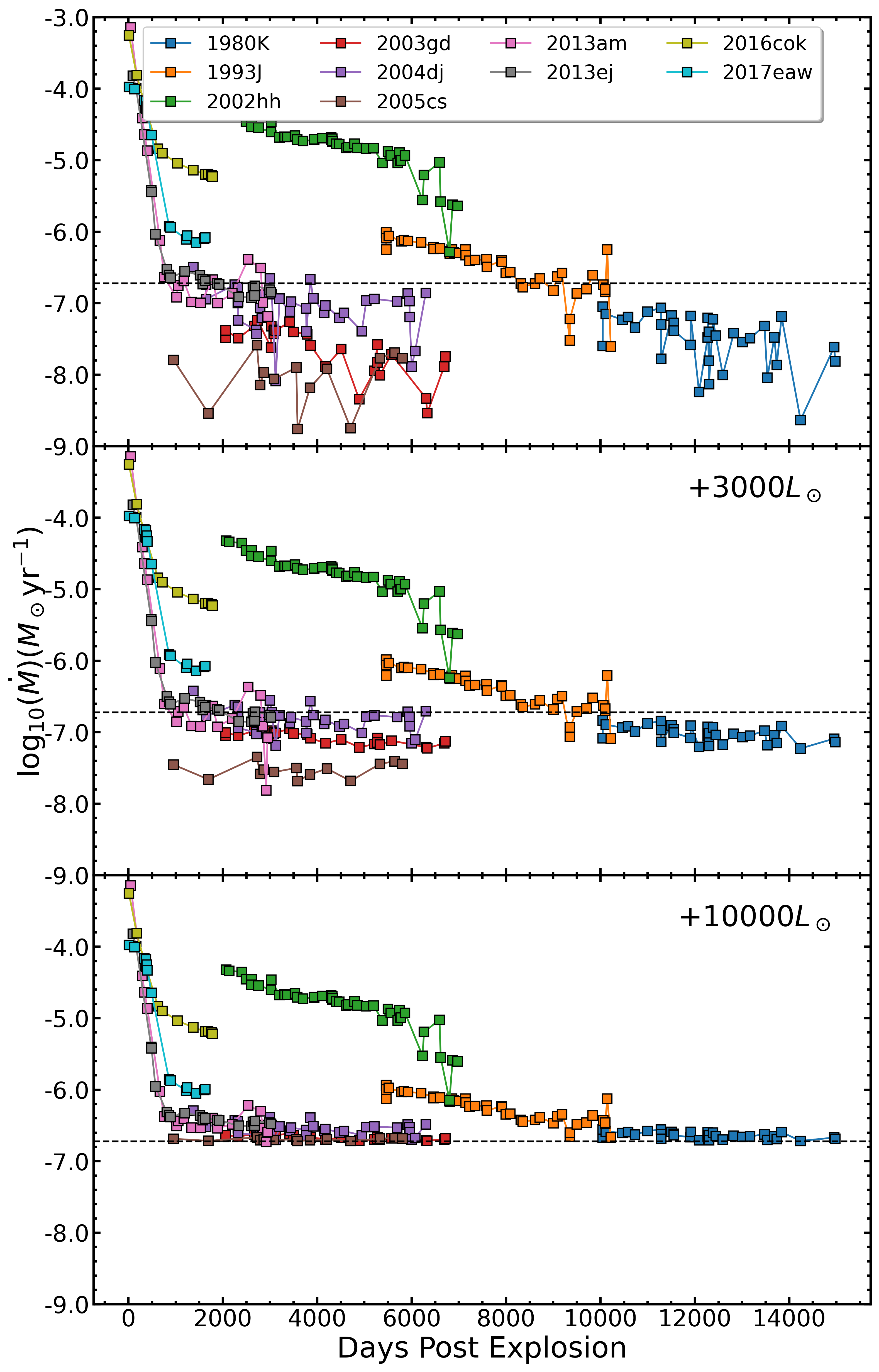
Figure 12: Pre-SN mass loss rates required to produce the observed R band luminosity after scaling $\nu L_{\nu}$ after adding zero (top), 3000L_⊙ (middle), and 10000L_⊙ (bottom) for the flux in the reference image. The dashed line represents a $\dot{M}$ corresponding to a luminosity of $10^{4}$L_⊙.

3.4 Dust Echoes

Using the same procedures as in §3.3 and Eqn. 6 yields the optical depth estimates given in Table 4. The required optical depths are not very large. We can recast Eqn. 6 using $E_{rad}=L_{peak}t_{peak}$ where $L_{peak}\sim 10^{8}L_{\odot}$ is the peak luminosity and $t_{peak}\simeq 100$ days is the duration of the plateau phase, so that $\tau\sim(L_{SN}/L_{peak})(t_{0}/t_{peak})$. The luminosity has dropped by $L_{SN}/L_{peak}\sim 10^{4}$ or more, while the elapsed time is only $t_{0}\sim 30t_{peak}$, leading to required optical depths of $\tau\sim 10^{-3.5}$-$10^{-2.5}$. However, as illustrated in Fig. 13, the shapes of the light curves generally show phases with the optical depth increasing with time. We also see in Figure 3 that the colors of the late time emission are different from the expectations for dust echoes. The dust echo colors should, essentially, be the colors of the SN shifted roughly parallel to the isochrones while the observed colors are generally shifted perpendicular to the isochrones. These facts appear to rule out dust echoes as a general explanation of the late time emission.

At first glance, these low required optical depths might seem to require significant dust echoes from essentially all the SNe because the required optical depths are much lower than the extinction estimates in Table 1 since $\tau_{R}\simeq 2.3E(B-V)$. The missing element is that the dust echo at any given time is being produced by a very thin region of thickness $\sim ct_{peak}\sim 0.1$ pc corresponding to the spatial extent of the luminosity transient. If the dust is uniformly distributed over a line of sight distance of 0.1 to 1 kpc, the optical depth scale relevant to producing an echo is fraction $10^{-3}$ to $10^{-4}$ of the total along the line of sight. Concentrating the dust in “sheets” helps, but more at early times when the physical region producing the echo is small. This discussion assumes unresolved echoes where the surface brightness of the echo is not relevant to its detection.

The exception is SN 2002hh which is both heavilty obscured (Table 1) and known to have a strong dust echo (e.g., Barlow et al. 2005, Pozzo et al. 2006, Welch et al. 2007, and Otsuka et al. 2012). With the large corrections for extinction, SN 2002hh has the greatest late-time luminosity of any of the 12 systems by almost two orders of magnitude. While it is fading in the R band, and evolving little in the B and V bands, the U band luminosity is clearly increasing. It is the only such system.

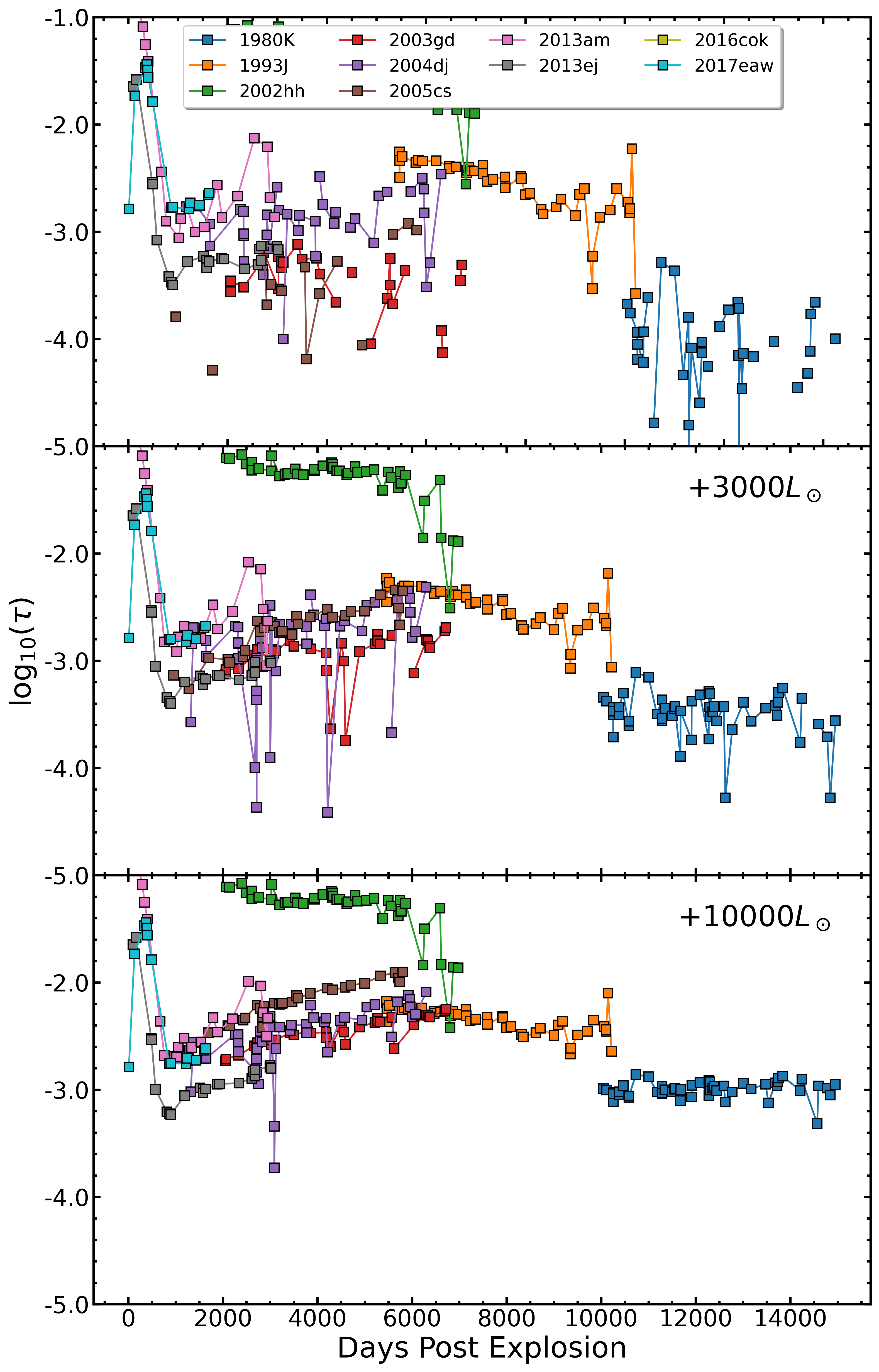
Figure 13: Required scattering optical depth $\tau$ (Eqn. 6) for the observed R band luminosity (V band for SN 1980K) after adding zero (top), 3000L_⊙ (middle), and 10000L_⊙ (bottom) for the flux in the reference image.

3.5 Binary Shock Interaction

We only consider the Type Ib/c SN 2012fh for this case because the progenitors of all the other SNe should be giants where it is impossible to significantly heat a main sequence companion as they subtend such a small solid angle. The companion star to a stripped SN should generally be a cooler star and dominate the optical emission even before being heated, so we assume that we can neglect the effect of the progenitor luminosity on the subtracted light curves. Under these assumptions, we estimate that a companion can have increased in luminosity by no more than $L_{max}\simeq 10^{5}L_{\odot}$ (Eqn. 11). Based on Fig. 10, SN 2012fh faded within ${\sim}$440 days after peak luminosity, which we use as our limit on the inflation time scale $\tau_{infl}$ (Eqn. 12). Fig. 14 translates these limits into the allowed companion mass $M_{c}$ and radius relative to the binary semi-major axis $R_{c}/a$.

Using Solar metallicity PARSEC isochrone with $\log_{10}$(Age) = 6.7, for which no $M_{c}<20M_{\odot}$ companions have evolved, we also show curves with constant semi-major axes of $a=50R_{\odot}$, $100R_{\odot}$ and $150R_{\odot}$ given the stellar radii $R_{c}$ of the models. At least for these models, the binary would have to be wider separation than $50$-$100R_{\odot}$ at the time of the explosion. If the progenitor of SN 2012fh was stripped through binary interactions, then the mass-radius relations of the single-star PARSEC isochrones will be incorrect at some level.

Figure 14: Allowed binary companions for SN 2012fh. The gray region excludes companions on their predicted inflation timescales and maximum luminosity. The brown, red, and orange dot-dashed lines represent orbital separations of 50, 100, and 150 R_⊙ respectively, with stellar counterpart masses and radii obtained from a solar metalicity, PARSEC isochrone with an age of $10^{6.7}$ years. This age is selected so that M$<20M_{\odot}$ have not yet evolved off the main sequence.

4 Conclusions

Motivated by the discovery that SN 2013am and SN 2013ej were still optically brighter than their progenitors a decade after explosion (Neustadt et al. 2021), we systematically investigated the evolution over the last 14 years of the 12 ccSNe that occurred in the LBT search for failed SNe (Kochanek et al. 2008a, Gerke et al. 2015, Adams et al. 2017a, Adams et al. 2017b, Basinger et al. 2021, Neustadt et al. 2021) galaxies from 1980 onwards. We used difference imaging techniques to look for continued evolution in their UBVR luminosities. Difference imaging has the advantage of largely eliminating the problem of crowding in these ground based data, but some quantitative conclusions depend on the difficult to estimate flux of the targets in the reference image. As part of the survey, we analyzed the SED of the progenitor of SN 2011dh from the LBT data and find results consistent with the results from pre-SN HST data (Van Dyk et al. 2011, Maund et al. 2011). This analysis also demonstrates that the LBT easily has the sensitivity to probe emissions at the level of $\sim 10\%$ of the progenitor luminosity or better (see Fig. 11). We also considered shock heated binary companions to the Type Ibc SN 2012fh and set limits on the companion mass $M_{c}$ and the ratio of the companion radius to the semi-major axis $R_{c}/a$ (see Fig. 14).

We focus these conclusions on the interesting finding that of the 11 Type II SNe in the sample, only two (the Type IIP SN 2005cs and the Type IIb SN 2011dh), do not show continued, evolving SN emission 5-42 years post-explosion. This includes the two oldest systems studied, the Type IIL SN 1980K and the Type IIb SN 1993J. The continued emission is coincidentally on the scale of the luminosity of the progenitors ($\sim 10^{4}L_{\odot}$). For the 6 of these SNe that occured after the LBT survey started, we know this is true of five (the exception is SN 2011dh) because we constructed the reference image from pre-SN images so that the luminosities in the subtracted light curves are relative to the luminosity of the progenitor. Apparently, SN like SN 1987A (e.g., Woosley 1988, Fransson et al. 2007, Seitenzahl et al. 2014) or SN 2011dh which rapidly fade to luminosities well below those of their progenitors are the exceptions, not the norm.

For completeness, we considered radioactivity, CSM interactions, dust echoes and magnetar/engines as possible drivers. Radioactivity requires impossible masses and dust echoes generally require too much dust. Neutron star spin down can produce the necessary luminosity, but is not believed to produce significant optical emission at these phases (e.g., Kasen & Bildsten 2010), which is certainly true of the Crab pulsar today. The time evolution of the luminosity and the colors of the emission are also generally inconsistent with dust echoes. Not surprisingly, since CSM emission has been observed at earlier phases for many of these sources (see Table 4 and Appendix A), the only logical possibility is continuing CSM emission aside from SN 2022hh where it is probably due to a very strong, continuing dust echo.

Mass loss is a crucial component of RSG evolution (e.g., Reimers 1975, de Jager et al. 1988, Nieuwenhuijzen & de Jager 1990, van Loon et al. 2005, Mauron & Josselin 2011, Beasor et al. 2021). If we use the progenitor luminosity scaling from Eqn. 2, we can express the Nieuwenhuijzen & de Jager (1990) mass loss rate as

$$\dot{M}=10^{-5.60}\left(\frac{M}{10M_{\odot}}\right)^{2.62}\left(\frac{T_{e}}{3500\hbox{K}}\right)^{-1.61}M_{\odot}~{}\hbox{yr}^{-1}$$ (13)

and the van Loon et al. (2005) mass loss rate as

$$\dot{M}=10^{-4.81}\left(\frac{M}{10M_{\odot}}\right)^{1.58}\left(\frac{T_{e}}{3500\hbox{K}}\right)^{-6.3}M_{\odot}~{}\hbox{yr}^{-1}.$$ (14)

With the temperature fixed at $3500$ K, the mass loss rates for $8M_{\odot}<M<20M_{\odot}$ span $-5.9<\log\dot{M}<-4.8$ and $-5.6<\log\dot{M}<-4.8$. These estimates are somewhat higher than our estimates in Table 4. While there are significant quantitative uncertainties in these estimates, particularly through the assumed shock velocity ($v_{s}=4000$ km/s) and the radiative efficiency ($\epsilon=0.1$) it would be difficult to significantly raise them given the lack of large numbers of X-ray bright Type II SNe (see Dwarkadas 2014). There are also arguments that these models for RSG mass loss rates are too high (e.g., Beasor et al. 2021).

Nonetheless, if we use these mass loss rates to predict the CSM luminosity (Eqn. 5) relative to the progenitor luminosity (Eqn. 2), we find that

$$\frac{L_{shock}}{L_{prog}}=2.09\left(\frac{\epsilon}{0.1}\right)\left(\frac{M}{10M_{\odot}}\right)^{1.12}\left(\frac{T}{3500~{}\hbox{K}}\right)^{-1.61}\\ \times\left(\frac{v_{s}}{4000~{}\hbox{km/s}}\right)^{3}\left(\frac{10~{}\hbox{km/s}}{v_{w}}\right)$$ (15)

and

$$\frac{L_{shock}}{L_{prog}}=12.9\left(\frac{\epsilon}{0.1}\right)\left(\frac{M}{10M_{\odot}}\right)^{0.08}\left(\frac{T}{3500~{}\hbox{K}}\right)^{-6.3}\\ \times\left(\frac{v_{s}}{4000~{}\hbox{km/s}}\right)^{3}\left(\frac{10~{}\hbox{km/s}}{v_{w}}\right)$$ (16)

for the two mass loss prescriptions. Since the luminosity of an RSG progenitor in a particular band is less than $L_{prog}$, it is clear that CSM emission from normal RSG winds can easily exceed the band luminosity of the progenitor provided the efficiency of converting the shock luminosity into optical emission is $\epsilon\mathrel{\raise 1.29167pt\hbox{$>$}\mkern-14.0mu\lower 2.58334pt\hbox{$\sim$}}0.01$. The interesting question then becomes the duration of the emission, since we generically find that the emissions are fading. One possibility, requiring theoretical study, is the physics of the efficiency $\epsilon$. While the shock luminosity for a fixed shock velocity is constant for a $1/r^{2}$ wind density, it would still be fairly natural for $\epsilon$ to evolve since most emission mechanisms scale as the square of the density rather than being proportional to the density like the shock luminosity. The fading could also be due to having wind density profiles that are generically steeper than the $1/r^{2}$ density profile of a constant $\dot{M}$ wind (see, e.g., Dwarkadas & Gruszko 2012).

The missing element for making these conclusions more quantitative is to obtain absolute calibrations. Waiting for the SN to fade to black seems to require challenging levels of patience given that SN 1980K seems to still be going strong. On the other hand, SN 1993J does appear to be close to fading away. Fortunately, single orbit HST observations can provide the necessary absolute flux levels for two to three filters depending on the desired level of control over systematic problems (cosmic rays, bad pixels etc.). For two filters, the preferred choices are probably R and B given the properties of observed (Matheson et al. 2000a) and theoretical (Dessart & Hillier 2022) spectra of CSM interactions, with adding V if a third filter is included.

The SN shock also eventually reaches the edge of the wind. In the Weaver (1976) self-similar solution for a wind expanding into a constant density medium, the contact discontinuity between the two fluids lies at

$$R_{CD}=5.4\left(\frac{\dot{M}}{10^{-6}M_{\odot}\hbox{yr}^{-1}}\right)^{1/5}\left(\frac{v_{w}}{10~{}\hbox{km/s}}\right)^{2/5}\\ \times\left(\frac{t}{10^{6}~{}\hbox{yr}}\right)^{3/5}\left(\frac{\hbox{cm}^{-3}}{n}\right)^{1/5}~{}\hbox{pc}$$ (17)

where $n$ is the ambient density and $t$ is the time since the start of the wind. Except for time, the parameter dependence is weak, so the time scale for the SN shock to reach the contact discontinuity is in unfortunately long ($1300$ years for $v_{s}=4000$ km/s). Moreover, the RSG wind may be expanding into a lower density bubble formed by a faster main sequence wind, leading to a still more distant contact discontinuity (e.g., Dwarkadas 2005). The wind termination shock can lie at a significantly smaller radius than the contact discontinuity, but centuries are not much of a gain over millennia.

Even if it seems unlikely that we will observe these boundaries of the RSG wind, it is still of interest to both continue to observe the evolution of these SNe and to extend the study to the small numbers of still older historical SNe in the LBT galaxies. Moreover, the estimated time scale to reach the edge of the wind is just an estimate – in SN 1987A, the shock started to interact with the wind boundary after only 20 years (e.g., Larsson et al. 2019). SN 2002hh is postulated to have a massive ($\sim 0.1M_{\odot}$) dusty shell at a distance of $0.03$ to $0.3$ pc (e.g., Barlow et al. 2005). Like (Andrews et al., 2015), we see no evidence for interactions with the postulatedshell, which leads to a minimum distance to the shell of $0.08(v_{s}/4000~{}\hbox{km/s})$ pc that begins to strongly constrain these models. And, since they are all fading, it will eventually be possible to do the progenitor photometry of those SNe with pre-explosion LBT imaging - just after far more time than expected.

Data Availability

The data underlying this article will be shared on reasonable request to the corresponding author.

Appendix A Individual Supernovae

Here we summarize the individual SNe. Table 1 lists the SN and gives the adopted distances, Galactic and host extinctions. Table 2 lists HST observations that can be used to provide absolute calibrations of the LBT light curves, and Table 4 gives previous estimates of mass loss rates $\dot{M}$.

SN 1980K

The Type II-L SN 1980K was discovered in NGC 6946 (Wild & Barbon, 1980) on 1980 October 28 reaching a maximum of $V=11.4$ mag on November 3 1980 (Barbon et al., 1982) and has been extensively studied far into the nebular phase (e.g., Chevalier 1982b Dwek 1983, Montes et al. 1998, Fesen & Becker 1990, Leibundgut et al. 1991, Chevalier & Fransson 1994, Milisavljevic et al. 2012). Based on the radio emission, Chevalier (1982b) estimated a rough mass loss rate of $\dot{M}\sim 10^{-5}M_{\odot}$ year^-1 for $v_{w}=10$ km/s, and Montes et al. (1998) argue for a break to a region with a lower wind density due to a sudden drop in the radio fluxes around 1995. Dwek (1983) argued for a dust echo from a shell formed at the wind/ISM boundary with a detailed model in Sugerman et al. (2012) placing the shell $\sim 15$ pc from the SN. They find weak evidence for optical fading between 2005 and 2008 and strong evidence for an infrared excess. The source they identify as the SN is clearly visible in the first LBT images, taken 4 months after the Sugerman et al. (2012) HST observations in January 2008. The LBT observations of NGC 6946 now span 13 years with approximately 57 epochs per filter.

SN 1993J

SN 1993J in M81 is the prototype of the Type IIb SNe class (Suzuki et al. 1993, Schmidt et al. 1993, Filippenko et al. 1993, Nomoto et al. 1993, Filippenko et al. 1994). It was discovered on 1993 March 28 (Ripero et al., 1993). Using ground based observations obtained prior to the SN, the progenitor of 1993J was identified as K0 RSG (Aldering et al., 1994), and its eventual disappearance has been observed (Maund & Smartt, 2009). The progenitor was not variable by more than 0.2 mag (Suzuki & Nomoto 1995). There is extensive evidence for CSM emission from late time spectra (e.g., Matheson et al. 2000b, Matheson et al. 2000c), X-ray emission (e.g., Suzuki et al. 1993, Leising et al. 1994, Suzuki & Nomoto 1995, Fransson et al. 1996, Kundu et al. 2019), and radio emission (e.g., van Dyk et al. (1994), Kundu et al. 2019). VLBI observations monitored the expansion of the remnant for almost a decade (Bietenholz et al., 2003), tracking the expansion to 19,000 AU (0.1 pc) and implying average expansion velocities of $\sim 10^{4}$ km/s. The Kundu et al. (2019) models assume a mass loss rate of $\dot{M}=4\times 10^{-5}M_{\odot}$/year before $3000$ days. The LBT observations of M81 now span ${\sim}$14 years with approximately 32 epochs per filter. For SN 1993J, the HST observations of Fox et al. (2014) provide an absolute calibration of the V and R band light curves (Table 2).

SN 2002hh

SN 2002hh is a Type IIP SN first discovered on 2002 October 31.1 (Li, 2002) by LOSS in NGC 6946. Barlow et al. (2005) argue for a massive ($\sim 0.1M_{\odot}$) dusty shell at a distance of $\sim 0.04$ pc, and the dust echoes are discussed further in Pozzo et al. (2006), Welch et al. (2007), and Otsuka et al. (2012). Andrews et al. (2015) spectroscopically searched for any evidence of shock interactions with such a dusty shell in 2013, 10.5 years after explosion, finding none. The spectra appear similar to the SN near peak, suggesting that the emission is dominated by a dust echo. We can use the HST observations from Otsuka et al. (2012) to normalize some of the LBT bands (Table 2). This galaxy has been observed by the LBT since mid-2008 with a total of 57 epochs in each filter.

SN 2003gd

SN 2003gd is a Type IIP SN discovered in NGC 628 (M 74) on 2003 June 12.82 (Evans & McNaught, 2003) with a general study in Hendry et al. (2005). Archival Hubble Space Telescope (HST) and Gemini data identified its progenitor, a RSG star with an estimated mass of $8^{+4}_{-2}M_{\odot}$ (Smartt et al. 2004, Hendry et al. 2005) and the progenitor is observed to have disappeared (Maund & Smartt 2009, Maund et al. 2014). Two years after explosion it had a faint, resolved (by HST) dust echo with $\sim 1\%$ of the optical flux of the SN (Sugerman, 2005). This galaxy has been observed for a total of 32 epochs.

SN 2004dj

SThe Type IIP SN 2004dj was discovered on 2004 July 31.76 in NGC 2403 (Nakano et al., 2004) with early observations in Vinkó et al. (2006), Tsvetkov et al. (2008) and Zhang et al. 2009 with extensions to $\sim 1000$ days in Vinkó et al. (2009). Van Dyk et al. (2003) and Maund & Smartt (2005) identify two progenitor candidates, and Maíz-Apellániz et al. 2004 and Vinkó et al. 2009 estimate a mass of $\sim 15M_{\odot}$ based on the age of the associated star cluster, Sandage 96. There is evidence of CSM emission from early optical spectroscopy, late-time X-ray, and radio observations (Chugai et al. 2007, Chakraborti et al. 2012, Nayana et al. 2018). Mid-IR Spitzer observations, late time optical photometry, and HST data from days $\sim 106-1393$ after explosion provide evidence for dust formation in the ejecta (Szalai et al. 2011, Meikle et al. 2011). There are 52 LBT epochs for NGC 2403.

SN 2005cs

SN 2005cs is a Type IIP SN in NGC 5194 (M 51) that was discovered on 2005 July 28.9 (Kloehr et al., 2005). There are general observations of SN 2005cs in Pastorello et al. (2006), Brown et al. 2007 and Pastorello et al. (2009). Based on archival HST and Gemini images, the progenitor was identified as a K3 RSG, with an approximate mass of $(8\pm 2)M_{\odot}$ (Maund et al., 2005; Li et al., 2006). Early UV, optical, and a non-detection in the X-rays provide an upper limit of $\dot{M}\mathrel{\raise 1.29167pt\hbox{$<$}\mkern-14.0mu\lower 2.58334pt\hbox{$\sim$}}10^{-5}M_{\odot}$/year on the pre-SN mass loss rate (Brown et al. 2007). There are 31 LBT epochs for NGC 5194.

SN 2009hd

SN 2009hd occurred in NGC 3627 (M66) on 2009 July 2.69 (Monard, 2009) and was classified as a Type IIL (Elias-Rosa et al., 2011). This SN is located in a region with very high host extinction (see Table 1). Elias-Rosa et al. (2011) reports an upper limit on the luminosity of the progenitor of $L_{bol}\lesssim 10^{5.04}L_{\odot}$ which we can use as an upper limit on the contributions of the progenitor to the reference image. The image subtraction residuals near the SN are unusually large, so while we have 27 LBT epochs, four of which were taken pre-outburst, the quantitative results are not very useful, particularly when combined with the high extinction.

SN 2011dh

SN 2011dh, was discovered in NGC 5914 (M51) on 2011 May 31.89 (Griga et al., 2011; Silverman et al., 2011) and classified as a Type IIb SN. There are general studies of SN 2011dh in Arcavi et al. (2011), Sahu et al. (2013), Ergon et al. (2014), and Ergon et al. (2015). The progenitor was yellow super-giant (YSG) (Maund et al. 2011, Van Dyk et al. 2011) with properties discussed in §3.1 and it appears to have been slightly variable (Szczygieł et al. 2012). Folatelli et al. 2014 argue that blue star detected in deep Near-UV HST images is a binary companion to the progenitor, but this is disputed by Maund et al. (2015). X-ray (Maeda et al. 2014) and radio (Soderberg et al. 2012) observations found evidence for CSM interactions, with a mass loss rate of order $\dot{M}\sim 3\times 10^{-6}M_{\odot}$/year for $v_{w}=20$ km/s. VLBI observations monitored the expansion of the remnant to a linear radius of $(7.4\pm 0.3)\times 10^{16}$cm implying an average expansion velocity of $\sim 19000$ km/s (de Witt et al., 2016). We have five observations before the SN and 26 afterwards, for a total of 31 LBT epochs.

SN 2012fh

This system was discovered on 2012 October 18.856 (Nakano et al., 2012) in NGC 3344, and was classified as a Type Ic by Tomasella et al. (2012) and Takaki et al. (2012). As in Johnson et al. (2017), we will use a more generic Type Ibc classification because the spectra were collected long after peak. Photometry for 2102fh is available in Shivvers et al. (2019) and Zheng et al. (2022). Johnson et al. (2017) place limits on the luminosity of the progenitor, finding that it likely had to be a lower mass star stripped by binary interactions. We have 10 LBT epochs prior to the SN and 16 afterwards for a total of 26 epochs This SN is the only candidate for which a binary companion analysis is carried out.

SN 2013am

This Type II-P SN was discovered on 2013 Mar. 21.638 in NGC 3623 by Nakano et al. (2013) and classified as a young Type II SN (Benetti et al., 2013). There are a general studies of it in Zhang et al. (2014) and Tomasella et al. (2018), additional light curve data in Galbany et al. (2016) and de Jaeger et al. (2019) and additional spectra in Silverman et al. (2017). The spectrum in Silverman et al. (2017) at $257$ days appears to be developing the box-shaped line profiles typical of CSM interactions. We have 8 pre-SN epochs of LBT data, one just 5 days before the discovery, and 29 epochs in total.

SN 2013ej

This SN was discovered on 2013 July 24.83 by Lee et al. (2013) in NGC 628 (M74) and classified as a young Type II (Kim et al., 2013). It is generally discussed in Valenti et al. (2014), Huang et al. (2015), Huang et al. (2015), Dhungana et al. 2016 and Yuan et al. (2016) where the latter argues that it should be classified as a Type IIL rather than a Type IIP. Fraser et al. (2014) argue that a red source in archival HST images might be the progenitor. Early optical observations (Bose et al. 2015), X-ray observations (Chakraborti et al. 2016) and spectropolarimetry (Mauerhan et al. 2017) all support the presence of CSM interactions. We have 13 pre-SN epochs of LBT data and 35 in total.

ASASSN-16fq/SN 2016cok

ASAS-SN (Shappee et al., 2014; Kochanek et al., 2017a) discovered the Type II-P SN ASASSN-16fq (SN 2016cok) in NGC 3627 (M66) on 2016 May 28.30 Bock et al. (2016). There is photometry of this SN in de Jaeger et al. (2019). Kochanek et al. (2017b) estimate that the progenitor was a $8-12M_{\odot}$ RSG with a luminosity of $10^{4.5}$ - $10^{4.9}$ and that it had no significant pre-SN variability. The SN was not detected in 23 ksec of Swift observations, but there is no discussion of the implications (Bock et al. 2016). We have 16 LBT epochs of pre-SN LBT data, and 26 in total.

SN 2017eaw

SN 2017eaw is a Type II-P discovered on 2017 May 14.24 (Wiggins, 2017; Dong & Stanek, 2017) in NGC 6946. There are general studies of the SN and its progenitor in Kilpatrick & Foley (2018), Van Dyk et al. (2019), and Szalai et al. (2019). There is additional photometry in Buta & Keel (2019) and evidence for dust formation after the explosion (Rho et al. 2018, Tinyanont et al. 2019). Late time spectra show clear evidence of CSM interactions (Weil et al. 2020). The progenitor luminosity is roughly $10^{4.9}L_{\odot}$ with a dusty wind or shell (Kilpatrick & Foley 2018). The 40 pre-SN LBT observations have no evidence for optical variability from the progenitor over its last roughly decade (Johnson et al. 2018b), which essentially rules out suggestions for late pre-SN outbursts (Kilpatrick & Foley 2018, Rui et al. 2019). We have 40 pre-SN LBT epochs, and a total of 54.

References

- Adams & Kochanek (2015) Adams S. M., Kochanek C. S., 2015, MNRAS, 452, 2195
- Adams et al. (2017a) Adams S. M., Kochanek C. S., Gerke J. R., Stanek K. Z., Dai X., 2017a, MNRAS, 468, 4968
- Adams et al. (2017b) Adams S. M., Kochanek C. S., Gerke J. R., Stanek K. Z., 2017b, MNRAS, 469, 1445
- Ahn et al. (2012) Ahn C. P., et al., 2012, ApJS, 203, 21
- Alard (2000) Alard C., 2000, A&AS, 144, 363
- Alard & Lupton (1999) Alard C., Lupton R., 1999, ISIS: A method for optimal image subtraction (ascl:9909.003)
- Aldering et al. (1994) Aldering G., Humphreys R. M., Richmond M., 1994, AJ, 107, 662
- Andrews et al. (2015) Andrews J. E., Smith N., Mauerhan J. C., 2015, MNRAS, 451, 1413
- Arcavi et al. (2011) Arcavi I., et al., 2011, ApJ, 742, L18
- Barbon et al. (1982) Barbon R., Ciatti F., Rosino L., 1982, A&A, 116, 35
- Barlow et al. (2005) Barlow M. J., et al., 2005, ApJ, 627, L113
- Baron et al. (2007) Baron E., Branch D., Hauschildt P. H., 2007, ApJ, 662, 1148
- Basinger et al. (2021) Basinger C. M., Kochanek C. S., Adams S. M., Dai X., Stanek K. Z., 2021, MNRAS, 508, 1156
- Beasor et al. (2021) Beasor E. R., Davies B., Smith N., 2021, ApJ, 922, 55
- Benetti et al. (2013) Benetti S., Tomasella L., Pastorello A., Cappellaro E., Turatto M., Ochner P., 2013, The Astronomer’s Telegram, 4909, 1
- Bevan et al. (2017) Bevan A., Barlow M. J., Milisavljevic D., 2017, MNRAS, 465, 4044
- Bietenholz et al. (2003) Bietenholz M. F., Bartel N., Rupen M. P., 2003, ApJ, 597, 374
- Bock et al. (2016) Bock G., et al., 2016, The Astronomer’s Telegram, 9091, 1
- Bose et al. (2015) Bose S., et al., 2015, ApJ, 806, 160
- Bressan et al. (2012) Bressan A., Marigo P., Girardi L., Salasnich B., Dal Cero C., Rubele S., Nanni A., 2012, MNRAS, 427, 127
- Brown et al. (2007) Brown P. J., et al., 2007, ApJ, 659, 1488
- Buta & Keel (2019) Buta R. J., Keel W. C., 2019, MNRAS, 487, 832
- Castelli & Kurucz (2003) Castelli F., Kurucz R. L., 2003, IAU Symposium, 210, A20
- Chakraborti et al. (2012) Chakraborti S., Yadav N., Ray A., Smith R., Chandra P., Pooley D., 2012, ApJ, 761, 100
- Chakraborti et al. (2016) Chakraborti S., et al., 2016, ApJ, 817, 22
- Chandra et al. (2022) Chandra P., Chevalier R. A., James N. J. H., Fox O. D., 2022, MNRAS, 517, 4151
- Chevalier (1982a) Chevalier R. A., 1982a, ApJ, 258, 790
- Chevalier (1982b) Chevalier R. A., 1982b, ApJ, 259, 302
- Chevalier (1986) Chevalier R. A., 1986, ApJ, 308, 225
- Chevalier & Fransson (1994) Chevalier R. A., Fransson C., 1994, ApJ, 420, 268
- Chevalier et al. (2006) Chevalier R. A., Fransson C., Nymark T. K., 2006, ApJ, 641, 1029
- Chugai et al. (2007) Chugai N. N., Chevalier R. A., Utrobin V. P., 2007, ApJ, 662, 1136
- Dessart & Hillier (2022) Dessart L., Hillier D. J., 2022, A&A, 660, L9
- Dhungana et al. (2016) Dhungana G., et al., 2016, ApJ, 822, 6
- Dong & Stanek (2017) Dong S., Stanek K. Z., 2017, The Astronomer’s Telegram, 10372, 1
- Dwarkadas (2005) Dwarkadas V. V., 2005, ApJ, 630, 892
- Dwarkadas (2014) Dwarkadas V. V., 2014, MNRAS, 440, 1917
- Dwarkadas & Gruszko (2012) Dwarkadas V. V., Gruszko J., 2012, MNRAS, 419, 1515
- Dwek (1983) Dwek E., 1983, ApJ, 274, 175
- Elias-Rosa et al. (2011) Elias-Rosa N., et al., 2011, ApJ, 742, 6
- Elitzur & Ivezić (2001) Elitzur M., Ivezić Ž., 2001, MNRAS, 327, 403
- Ergon et al. (2014) Ergon M., et al., 2014, A&A, 562, A17
- Ergon et al. (2015) Ergon M., et al., 2015, A&A, 580, A142
- Evans & McNaught (2003) Evans R., McNaught R. H., 2003, IAU Circ., 8150, 2
- Fesen & Becker (1990) Fesen R. A., Becker R. H., 1990, ApJ, 351, 437
- Filippenko et al. (1993) Filippenko A. V., Matheson T., Ho L. C., 1993, ApJ, 415, L103
- Filippenko et al. (1994) Filippenko A. V., Matheson T., Barth A. J., 1994, AJ, 108, 2220
- Folatelli et al. (2014) Folatelli G., et al., 2014, ApJ, 793, L22
- Fox et al. (2014) Fox O. D., et al., 2014, ApJ, 790, 17
- Fransson et al. (1996) Fransson C., Lundqvist P., Chevalier R. A., 1996, ApJ, 461, 993
- Fransson et al. (2007) Fransson C., Gilmozzi R., Groeningsson P., Hanuschik R., Kjaer K., Leibundgut B., Spyromilio J., 2007, The Messenger, 127, 44
- Fraser et al. (2014) Fraser M., et al., 2014, MNRAS, 439, L56
- Fryxell & Arnett (1981) Fryxell B. A., Arnett W. D., 1981, ApJ, 243, 994
- Galbany et al. (2016) Galbany L., et al., 2016, AJ, 151, 33
- Gerke et al. (2011) Gerke J. R., Kochanek C. S., Prieto J. L., Stanek K. Z., Macri L. M., 2011, ApJ, 743, 176
- Gerke et al. (2015) Gerke J. R., Kochanek C. S., Stanek K. Z., 2015, Monthly Notices of the Royal Astronomical Society, 450, 3289–3305
- Giallongo et al. (2008) Giallongo E., et al., 2008, A&A, 482, 349
- Green et al. (2019) Green G. M., Schlafly E., Zucker C., Speagle J. S., Finkbeiner D., 2019, ApJ, 887, 93
- Griga et al. (2011) Griga T., et al., 2011, Central Bureau Electronic Telegrams, 2736, 1
- Groh et al. (2013) Groh J. H., Meynet G., Georgy C., Ekström S., 2013, A&A, 558, A131
- Guenther & Klose (2004) Guenther E. W., Klose S., 2004, IAU Circ., 8384, 3
- Hendry et al. (2005) Hendry M. A., et al., 2005, MNRAS, 359, 906
- Herrmann et al. (2008) Herrmann K. A., Ciardullo R., Feldmeier J. J., Vinciguerra M., 2008, ApJ, 683, 630
- Hill et al. (2006) Hill J. M., Green R. F., Slagle J. H., 2006, in Stepp L. M., ed., Society of Photo-Optical Instrumentation Engineers (SPIE) Conference Series Vol. 6267, Society of Photo-Optical Instrumentation Engineers (SPIE) Conference Series. p. 62670Y, doi:10.1117/12.669832
- Hirai et al. (2014) Hirai R., Sawai H., Yamada S., 2014, ApJ, 792, 66
- Hirai et al. (2018) Hirai R., Podsiadlowski P., Yamada S., 2018, ApJ, 864, 119
- Huang et al. (2015) Huang F., et al., 2015, ApJ, 807, 59
- Ivezic & Elitzur (1997) Ivezic Z., Elitzur M., 1997, MNRAS, 287, 799
- Ivezic et al. (1999) Ivezic Z., Nenkova M., Elitzur M., 1999, arXiv e-prints, pp astro–ph/9910475
- Johnson et al. (2017) Johnson S. A., Kochanek C. S., Adams S. M., 2017, MNRAS, 472, 3115
- Johnson et al. (2018a) Johnson S. A., Kochanek C. S., Adams S. M., 2018a, MNRAS, 480, 1696
- Johnson et al. (2018b) Johnson S. A., Kochanek C. S., Adams S. M., 2018b, MNRAS, 480, 1696
- Jordi et al. (2006) Jordi K., Grebel E. K., Ammon K., 2006, A&A, 460, 339
- Kanbur et al. (2003) Kanbur S. M., Ngeow C., Nikolaev S., Tanvir N. R., Hendry M. A., 2003, A&A, 411, 361
- Kaplan et al. (2008) Kaplan D. L., Chatterjee S., Gaensler B. M., Anderson J., 2008, ApJ, 677, 1201
- Karachentsev et al. (2000) Karachentsev I. D., Sharina M. E., Huchtmeier W. K., 2000, A&A, 362, 544
- Kasen & Bildsten (2010) Kasen D., Bildsten L., 2010, ApJ, 717, 245
- Kilpatrick & Foley (2018) Kilpatrick C. D., Foley R. J., 2018, MNRAS, 481, 2536
- Kim et al. (2013) Kim M., et al., 2013, Central Bureau Electronic Telegrams, 3606, 1
- Kloehr et al. (2005) Kloehr W., Muendlein R., Li W., Yamaoka H., Itagaki K., 2005, IAU Circ., 8553, 1
- Kochanek et al. (2008a) Kochanek C. S., Beacom J. F., Kistler M. D., Prieto J. L., Stanek K. Z., Thompson T. A., Yüksel H., 2008a, ApJ, 684, 1336
- Kochanek et al. (2008b) Kochanek C. S., Beacom J. F., Kistler M. D., Prieto J. L., Stanek K. Z., Thompson T. A., Yüksel H., 2008b, The Astrophysical Journal, 684, 1336–1342
- Kochanek et al. (2017a) Kochanek C. S., et al., 2017a, PASP, 129, 104502
- Kochanek et al. (2017b) Kochanek C. S., et al., 2017b, MNRAS, 467, 3347
- Kundu et al. (2019) Kundu E., et al., 2019, ApJ, 875, 17
- Larsson et al. (2019) Larsson J., et al., 2019, ApJ, 886, 147
- Lee et al. (2013) Lee M., et al., 2013, The Astronomer’s Telegram, 5466, 1
- Leibundgut et al. (1991) Leibundgut B., Kirshner R. P., Pinto P. A., Rupen M. P., Smith R. C., Gunn J. E., Schneider D. P., 1991, ApJ, 372, 531
- Leising et al. (1994) Leising M. D., et al., 1994, ApJ, 431, L95
- Li (2002) Li W., 2002, IAU Circ., 8005, 1
- Li et al. (2006) Li W., Van Dyk S. D., Filippenko A. V., Cuillandre J.-C., Jha S., Bloom J. S., Riess A. G., Livio M., 2006, ApJ, 641, 1060
- Liu et al. (2003) Liu J.-F., Bregman J. N., Seitzer P., 2003, ApJ, 582, 919
- Maeda et al. (2014) Maeda K., Katsuda S., Bamba A., Terada Y., Fukazawa Y., 2014, ApJ, 785, 95
- Maíz-Apellániz et al. (2004) Maíz-Apellániz J., Bond H. E., Siegel M. H., Lipkin Y., Maoz D., Ofek E. O., Poznanski D., 2004, ApJ, 615, L113
- Margutti et al. (2012) Margutti R., Soderberg A. M., Milisavljevic D., 2012, The Astronomer’s Telegram, 4544, 1
- Marietta et al. (2000) Marietta E., Burrows A., Fryxell B., 2000, ApJS, 128, 615
- Marigo et al. (2013) Marigo P., Bressan A., Nanni A., Girardi L., Pumo M. L., 2013, MNRAS, 434, 488
- Matheson et al. (2000a) Matheson T., et al., 2000a, AJ, 120, 1487
- Matheson et al. (2000b) Matheson T., et al., 2000b, AJ, 120, 1487
- Matheson et al. (2000c) Matheson T., Filippenko A. V., Ho L. C., Barth A. J., Leonard D. C., 2000c, AJ, 120, 1499
- Mauerhan et al. (2017) Mauerhan J. C., et al., 2017, ApJ, 834, 118
- Maund (2019) Maund J. R., 2019, ApJ, 883, 86
- Maund & Smartt (2005) Maund J. R., Smartt S. J., 2005, MNRAS, 360, 288
- Maund & Smartt (2009) Maund J. R., Smartt S. J., 2009, Science, 324, 486
- Maund et al. (2005) Maund J. R., Smartt S. J., Danziger I. J., 2005, MNRAS, 364, L33
- Maund et al. (2011) Maund J. R., et al., 2011, ApJ, 739, L37
- Maund et al. (2014) Maund J. R., Reilly E., Mattila S., 2014, MNRAS, 438, 938
- Maund et al. (2015) Maund J. R., et al., 2015, MNRAS, 454, 2580
- Mauron & Josselin (2011) Mauron N., Josselin E., 2011, A&A, 526, A156
- Meikle et al. (2002) Meikle P., Mattila S., Smartt S., MacDonald E., Clewley L., Dalton G., 2002, IAU Circ., 8024, 1
- Meikle et al. (2011) Meikle W. P. S., et al., 2011, ApJ, 732, 109
- Meng et al. (2007) Meng X., Chen X., Han Z., 2007, PASJ, 59, 835
- Milisavljevic et al. (2012) Milisavljevic D., Fesen R. A., Chevalier R. A., Kirshner R. P., Challis P., Turatto M., 2012, ApJ, 751, 25
- Monard (2009) Monard L. A. G., 2009, Central Bureau Electronic Telegrams, 1867, 1
- Montes et al. (1998) Montes M. J., Van Dyk S. D., Weiler K. W., Sramek R. A., Panagia N., 1998, ApJ, 506, 874
- Morozova et al. (2015) Morozova V., Piro A. L., Renzo M., Ott C. D., Clausen D., Couch S. M., Ellis J., Roberts L. F., 2015, ApJ, 814, 63
- Morozova et al. (2018) Morozova V., Piro A. L., Valenti S., 2018, ApJ, 858, 15
- Nadyozhin (1994) Nadyozhin D. K., 1994, ApJS, 92, 527
- Nakano et al. (2004) Nakano S., Itagaki K., Bouma R. J., Lehky M., Hornoch K., 2004, IAU Circ., 8377, 1
- Nakano et al. (2012) Nakano S., et al., 2012, Central Bureau Electronic Telegrams, 3263, 1
- Nakano et al. (2013) Nakano S., et al., 2013, Central Bureau Electronic Telegrams, 3440, 1
- Nayana et al. (2018) Nayana A. J., Chandra P., Ray A. K., 2018, ApJ, 863, 163
- Neustadt et al. (2021) Neustadt J. M. M., Kochanek C. S., Stanek K. Z., Basinger C., Jayasinghe T., Garling C. T., Adams S. M., Gerke J., 2021, MNRAS, 508, 516
- Nieuwenhuijzen & de Jager (1990) Nieuwenhuijzen H., de Jager C., 1990, A&A, 231, 134
- Nomoto et al. (1993) Nomoto K., Suzuki T., Shigeyama T., Kumagai S., Yamaoka H., Saio H., 1993, Nature, 364, 507
- Ogata et al. (2021) Ogata M., Hirai R., Hijikawa K., 2021, MNRAS, 505, 2485
- Otsuka et al. (2012) Otsuka M., et al., 2012, ApJ, 744, 26
- Pastorello et al. (2006) Pastorello A., et al., 2006, MNRAS, 370, 1752
- Pastorello et al. (2009) Pastorello A., et al., 2009, MNRAS, 394, 2266
- Podsiadlowski (2003) Podsiadlowski P., 2003, arXiv e-prints, pp astro–ph/0303660
- Poznanski et al. (2009) Poznanski D., et al., 2009, ApJ, 694, 1067
- Pozzo et al. (2006) Pozzo M., et al., 2006, MNRAS, 368, 1169
- Reimers (1975) Reimers D., 1975, Memoires of the Societe Royale des Sciences de Liege, 8, 369
- Rest et al. (2005) Rest A., et al., 2005, Nature, 438, 1132
- Rest et al. (2011) Rest A., Sinnott B., Welch D. L., Foley R. J., Narayan G., Mandel K., Huber M. E., Blondin S., 2011, ApJ, 732, 2
- Rho et al. (2018) Rho J., Geballe T. R., Banerjee D. P. K., Dessart L., Evans A., Joshi V., 2018, ApJ, 864, L20
- Richmond et al. (1994) Richmond M. W., Treffers R. R., Filippenko A. V., Paik Y., Leibundgut B., Schulman E., Cox C. V., 1994, AJ, 107, 1022
- Ripero et al. (1993) Ripero J., et al., 1993, IAU Circ., 5731, 1
- Rui et al. (2019) Rui L., et al., 2019, MNRAS, 485, 1990
- Sahu et al. (2013) Sahu D. K., Anupama G. C., Chakradhari N. K., 2013, MNRAS, 433, 2
- Sandberg & Sollerman (2009) Sandberg A., Sollerman J., 2009, A&A, 504, 525
- Schlafly & Finkbeiner (2011) Schlafly E. F., Finkbeiner D. P., 2011, ApJ, 737, 103
- Schmidt et al. (1993) Schmidt B. P., et al., 1993, Nature, 364, 600
- Seitenzahl et al. (2014) Seitenzahl I. R., Timmes F. X., Magkotsios G., 2014, ApJ, 792, 10
- Shappee et al. (2014) Shappee B. J., et al., 2014, ApJ, 788, 48
- Shivvers et al. (2019) Shivvers I., et al., 2019, MNRAS, 482, 1545
- Silverman et al. (2011) Silverman J. M., Filippenko A. V., Cenko S. B., 2011, The Astronomer’s Telegram, 3398, 1
- Silverman et al. (2017) Silverman J. M., et al., 2017, MNRAS, 467, 369
- Smartt et al. (2004) Smartt S. J., Maund J. R., Hendry M. A., Tout C. A., Gilmore G. F., Mattila S., Benn C. R., 2004, Science, 303, 499
- Soderberg et al. (2012) Soderberg A. M., et al., 2012, ApJ, 752, 78
- Sugerman (2003) Sugerman B. E. K., 2003, AJ, 126, 1939
- Sugerman (2005) Sugerman B. E. K., 2005, ApJ, 632, L17
- Sugerman & Crotts (2002) Sugerman B. E. K., Crotts A. P. S., 2002, ApJ, 581, L97
- Sugerman et al. (2012) Sugerman B. E. K., et al., 2012, ApJ, 749, 170
- Sukhbold et al. (2016) Sukhbold T., Ertl T., Woosley S. E., Brown J. M., Janka H. T., 2016, ApJ, 821, 38
- Suzuki & Nomoto (1995) Suzuki T., Nomoto K., 1995, ApJ, 455, 658
- Suzuki et al. (1993) Suzuki T., Kumagai S., Shigeyama T., Nomoto K., Yamaoka H., Saio H., 1993, ApJ, 419, L73
- Szalai et al. (2011) Szalai T., Vinkó J., Balog Z., Gáspár A., Block M., Kiss L. L., 2011, A&A, 527, A61
- Szalai et al. (2019) Szalai T., et al., 2019, ApJ, 876, 19
- Szczygieł et al. (2012) Szczygieł D. M., Gerke J. R., Kochanek C. S., Stanek K. Z., 2012, ApJ, 747, 23
- Takaki et al. (2012) Takaki K., Itoh R., Ueno I., Urano T., Moritani Y., Akitaya H., Kawabata K. S., Yamanaka M., 2012, Central Bureau Electronic Telegrams, 3263, 3
- Tinyanont et al. (2019) Tinyanont S., et al., 2019, ApJ, 873, 127
- Tomasella et al. (2012) Tomasella L., Turatto M., Benetti S., Pastorello A., Ochner P., Cappellaro E., 2012, Central Bureau Electronic Telegrams, 3263, 2
- Tomasella et al. (2018) Tomasella L., et al., 2018, MNRAS, 475, 1937
- Tsvetkov et al. (2007) Tsvetkov D. Y., Muminov M., Burkhanov O., Kahharov B., 2007, Peremennye Zvezdy, 27, 5
- Tsvetkov et al. (2008) Tsvetkov D. Y., Goranskij V., Pavlyuk N., 2008, Peremennye Zvezdy, 28, 8
- Valenti et al. (2014) Valenti S., et al., 2014, MNRAS, 438, L101
- Van Dyk et al. (2003) Van Dyk S. D., Li W., Filippenko A. V., 2003, PASP, 115, 1
- Van Dyk et al. (2011) Van Dyk S. D., et al., 2011, ApJ, 741, L28
- Van Dyk et al. (2019) Van Dyk S. D., et al., 2019, ApJ, 875, 136
- Van Dyk et al. (2022) Van Dyk S. D., et al., 2022, MNRAS,
- Verdes-Montenegro et al. (2000) Verdes-Montenegro L., Bosma A., Athanassoula E., 2000, A&A, 356, 827
- Vinkó et al. (2006) Vinkó J., et al., 2006, MNRAS, 369, 1780
- Vinkó et al. (2009) Vinkó J., et al., 2009, ApJ, 695, 619
- Weaver (1976) Weaver T. A., 1976, ApJS, 32, 233
- Weil et al. (2020) Weil K. E., Fesen R. A., Patnaude D. J., Milisavljevic D., 2020, ApJ, 900, 11
- Weiler et al. (1992) Weiler K. W., van Dyk S. D., Panagia N., Sramek R. A., 1992, ApJ, 398, 248
- Welch et al. (2007) Welch D. L., Clayton G. C., Campbell A., Barlow M. J., Sugerman B. E. K., Meixner M., Bank S. H. R., 2007, ApJ, 669, 525
- Wheeler et al. (1975) Wheeler J. C., Lecar M., McKee C. F., 1975, ApJ, 200, 145
- Wiggins (2017) Wiggins P., 2017, Central Bureau Electronic Telegrams, 4390, 1
- Wild & Barbon (1980) Wild P., Barbon R., 1980, IAU Circ., 3532, 1
- Willick et al. (1997) Willick J. A., Courteau S., Faber S. M., Burstein D., Dekel A., Strauss M. A., 1997, ApJS, 109, 333
- Woosley (1988) Woosley S. E., 1988, ApJ, 330, 218
- Wu & Fuller (2022) Wu S. C., Fuller J., 2022, ApJ, 930, 119
- Yuan et al. (2016) Yuan F., et al., 2016, MNRAS, 461, 2003
- Zhang et al. (2009) Zhang T.-M., Wang X.-F., Zhou X., Ma J., Jiang Z.-J., Wu J.-H., Wu Z.-Y., Basa S., 2009, Research in Astronomy and Astrophysics, 9, 783
- Zhang et al. (2014) Zhang J., et al., 2014, ApJ, 797, 5
- Zheng et al. (2022) Zheng W., et al., 2022, MNRAS, 512, 3195
- Zsíros et al. (2022) Zsíros S., Nagy A. P., Szalai T., 2022, MNRAS, 509, 3235
- de Jaeger et al. (2019) de Jaeger T., et al., 2019, MNRAS, 490, 2799
- de Jager et al. (1988) de Jager C., Nieuwenhuijzen H., van der Hucht K. A., 1988, A&AS, 72, 259
- de Witt et al. (2016) de Witt A., Bietenholz M. F., Kamble A., Soderberg A. M., Brunthaler A., Zauderer B., Bartel N., Rupen M. P., 2016, MNRAS, 455, 511
- van Dyk et al. (1994) van Dyk S. D., Weiler K. W., Sramek R. A., Rupen M. P., Panagia N., 1994, ApJ, 432, L115
- van Loon et al. (2005) van Loon J. T., Cioni M. R. L., Zijlstra A. A., Loup C., 2005, A&A, 438, 273