Lepton-flavour-violating tau decays from triality

Abstract

Motivated by flavour symmetry models, we construct theories based on a low-energy limit featuring lepton flavour triality that have the flavour-violating decays $\tau^{\pm}\to\mu^{\pm}\mu^{\pm}e^{\mp}$ and $\tau^{\pm}\to e^{\pm}e^{\pm}\mu^{\mp}$ as the main phenomenological signatures of physics beyond the standard model. These decay modes are expected to be probed in the near future with increased sensitivity by the Belle II experiment at the SuperKEKB collider. The simple standard model extensions featured have doubly-charged scalars as the mediators of the above decay processes. The phenomenology of these extensions is studied here in detail.

I Introduction

The search for charged-lepton flavour violation (cLFV) is an important component of the general program of seeking signals of physics beyond the standard model (BSM). The discovery of neutrino flavour oscillations established that the family lepton numbers $L_{e}$, $L_{\mu}$ and $L_{\tau}$ are not individually conserved. With the charged and neutral leptons coexisting in the same weak-isospin doublet, we thus expect that these quantities will also not be conserved in the charged-lepton sector. However, for such processes to be experimentally observable, lepton flavour violating (LFV) physics beyond that responsible for family-lepton number violating neutrino mass generation must exist.

There are stringent existing constraints on electron-muon cLFV processes such as $\mu\to e\gamma$ and $\mu\to eee$. Existing data on cLFV involving $\tau$ leptons are less constraining, but the sensitivity to such processes is expected to increase significantly as the Belle II experiment accumulates more data. The purpose of this paper is to construct and analyse some simple standard model (SM) extensions that have the decays

$$\tau^{\pm}\to\mu^{\pm}\mu^{\pm}e^{\mp},\qquad\tau^{\pm}\to\mu^{\mp}e^{\pm}e^{\pm}$$ (1)

as the main phenomenological signatures of BSM physics. We summarise the current bounds and projected Belle II sensitivities in Table 1.

Observable	Present constraint	Projected sensitivity
BR$(\tau^{-}\to\mu^{-}\mu^{-}e^{+})$	$<1.7\times 10^{-8}$ [1]	$2.6\times 10^{-10}$ [2]
BR$(\tau^{-}\to\mu^{+}e^{-}e^{-})$	$<1.5\times 10^{-8}$ [1]	$2.3\times 10^{-10}$ [2]

Table 1: We list the cLFV tau decays of interest, where the projected reach reflects the expected sensitivity with $50$ ab^-1 data from the Belle II collaboration [2] assuming a phase space distribution for the 3-body decay (see discussion in Sec. IV).

To achieve our aim, a symmetry is needed that permits the above decays but also prevents other processes that are subject to strong constraints. A simple choice for such a symmetry is lepton flavour triality. This has, for example, been discussed in the context of $A_{4}$ flavour models [3, 4, 5, 6, 7, 8, 9, 10, 11] which are broken to a $Z_{3}$ subgroup in the charged lepton sector and $Z_{2}$ in the neutrino sector.

Motivated by an eventual embedding into a more complete flavour symmetry model, we introduce a $Z_{3}$ symmetry in the lepton sector which distinguishes the three families via their $Z_{3}$ triality charges (denoted $T$). The first (second) [third] generation of leptons has charge $T=1$ ($2$) [$3$]. These charges correspond to the transformations

$$L\to\omega^{T}L,\quad e_{R}\to\omega^{T}e_{R}$$ (2)

where $\omega=e^{2\pi i/3}$ is the third root of unity, and the $L$ and $e_{R}$ are left-handed (LH) lepton doublets and right-handed (RH) charged lepton singlets, respectively. Thus all first-family leptons transform via $\omega$, all second-family leptons transform via $\omega^{2}$, and all third-family leptons are triality singlets, transforming via $\omega^{3}=1$. A discussion of neutrino masses is postponed to Sec. V. The Higgs doublet, $H$, and all quark fields are also triality singlets.

Given these triality assignments, the leptonic Yukawa terms in the Lagrangian are

$$\mathcal{L}\supset y_{ei}\bar{L}_{i}e_{Ri}H+\mathrm{h.c.},$$ (3)

where $i,j=1,2,3$ with repeated indices summed, and $y_{ei}$ denote the charged lepton Yukawa couplings. The $Z_{3}$ symmetry forces the charged lepton mass matrix to be diagonal, and we thus identify the first (second) [third] generation of charged leptons with the electron (muon) [tau] lepton.

This simple model outlined above forms the basis for extensions that feature observable decays of the form of Eq. (1). The simplest models are based on scalar bileptons [12], in particular doubly-charged scalars as illustrated in Fig. 1. In Sec. II we discuss the simplest realisation based on an electroweak singlet and in Sec. III we present a model based on an electroweak triplet. The phase space for the cLFV leptonic $\tau$ decays is discussed in Sec. IV and different possibilities to introduce neutrino masses are introduced in Sec. V and in Sec. VI we summarise and conclude. Technical details are reported in the appendices.

Figure 1: Tree-level contributions to the process $\tau^{-}\to\mu^{+}e^{-}e^{-}$ ($\tau^{-}\to\mu^{-}\mu^{-}e^{+}$) for the $T=1$ ($T=2$) electroweak singlet scalar models, utilising $k_{i}$, and triplet models, utilising $\Delta_{i}$. Note that the singlet models couple to RH leptons, whereas the triplets couple to LH leptons.

II Electroweak singlet models

The simplest model that has cLFV $\tau$ decays as the dominant BSM signature features a doubly-charged scalar weak-isospin singlet $k_{T}$ with lepton triality charge $T$, hypercharge $Y(k_{T})=2$ and a mass $m_{k_{T}}$. Depending on the lepton triality assignment for the doubly-charged scalar $k_{T}$, there are different cLFV $\tau$ decay modes. Note that we only consider $T=1$ and $T=2$, because the $T=0$ case does not result in cLFV $\tau$ decays.

II.1 $T=1$ singlet model

For triality $T=1$ the Yukawa couplings of the doubly-charged scalar $k_{1}$ are

$$\mathcal{L}_{k_{1}}=\frac{1}{2}\left(2f_{1}\overline{(\tau_{R})^{c}}\mu_{R}+f_{2}\overline{(e_{R})^{c}}e_{R}\right)k_{1}+\mathrm{h.c.}.$$ (4)

which induce the decays $\tau^{\pm}\to\mu^{\mp}e^{\pm}e^{\pm}$ via the LH diagram in Fig. 1. Note that we may, without loss of generality, set the coupling constants $f_{1,2}$ to be real-valued and positive, which we do from now on. One of the phases of $f_{1,2}$ may be absorbed into $k_{1}$, and the other absorbed into a RH charged lepton. Ultimately, the leptonic CP violation can be taken to reside entirely in the PMNS matrix and the decay modes of the heavy neutral leptons.

For energies below the mass of $k_{1}$, we can employ standard model effective field theory (SMEFT) and match to low-energy effective field theory (LEFT), the concepts and notation of which are reviewed in Appendices A and B. The LEFT Wilson coefficient for the relevant cLFV decay mode

$$C^{\rm VRR}_{ee,1312}=\frac{f_{1}f_{2}}{4m_{k_{1}}^{2}}$$ (5)

contributes to the branching ratio

$$\mathrm{BR}(\tau^{\pm}\to\mu^{\mp}e^{\pm}e^{\pm}) =\frac{f_{1}^{2}f_{2}^{2}}{64G_{F}^{2}m_{k_{1}}^{4}}\mathrm{BR}(\tau^{-}\to\mu^{-}\bar{\nu}_{\mu}\nu_{\tau}).$$ (6)

Applying the present constraint quoted in Table 1 and using Eq. (6), the following upper-bound results:

$$\sqrt{|f_{1}f_{2}|}\lesssim{0.17}\ \frac{m_{k_{1}}}{\text{TeV}}.$$ (7)

This constraint is shown by the diagonal solid coloured lines in top panels of Fig. 2 for the benchmark masses $m_{k_{1}}=1$ and $5$ TeV. The coupling constant parameter space to the top-right of these lines is ruled out. The coloured dot-dashed lines show the expected reach of the Belle II experiment. The grey bands in Fig. 2 display the regions for which the coupling constants are non-perturbative, and hence irrelevant for our analysis.

The benchmark masses were chosen to be within the range that would produce an observable cLFV branching ratio at Belle II. By saturating the perturbativity conditions (i.e. $f_{1}^{2}=f_{2}^{2}=4\pi$), the projected sensitivity quoted in Table 1 allows to probe $k_{1}$ masses:

$$m_{k_{1}}\lesssim{61}\;\;\text{TeV}.$$ (8)

Of course, for larger scalar masses the constraints considered become weaker, but so too does the observable effect in cLFV tau decays.

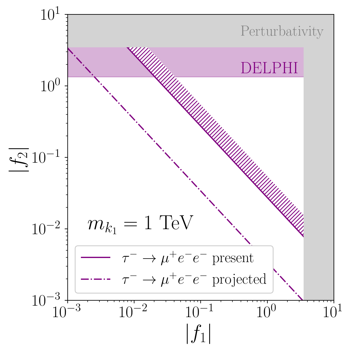
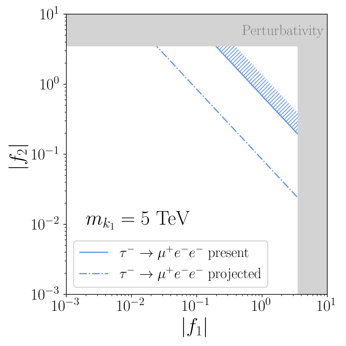
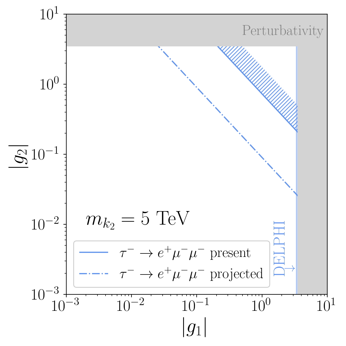
Figure 2: An overview of the electroweak singlet scalar parameter space. The present constraint on cLFV tau decays rules out the parameter space bounded by solid lines, in the direction of the hashing. The reach of Belle II is indicated by dot-dashed lines, i.e. observation of the decay $\tau^{-}\to\mu^{+}e^{-}e^{-}$ ($\tau^{-}\to e^{+}\mu^{-}\mu^{-}$) would be compatible with parameter space in the upper-right in the $|f_{1}|$-$|f_{2}|$ ($|g_{1}|$-$|g_{2}|$) plane above this line. The grey-shaded region is ruled-out by perturbativity of the BSM couplings. The shaded region labelled ‘DELPHI’ is ruled-out by the constraints in Eq. (18), and where this is absent the constraint falls outside the perturbative regime.

II.2 $T=2$ singlet model

For lepton triality $T=2$ the relevant Yukawa couplings in the Lagrangian of the doubly-charged scalar $k_{2}$ are obtained by exchanging the lepton flavours $1\leftrightarrow 2$ in the Lagrangian of Eq. (4), and are thus given by

$$\mathcal{L}_{k_{2}}=\frac{1}{2}\left(2g_{1}\overline{(\tau_{R})^{c}}e_{R}+g_{2}\overline{(\mu_{R})^{c}}\mu_{R}\right)k_{2}+\mathrm{h.c.}$$ (9)

where we have set $g_{1,2}$ to be real and positive, as per the discussion in Sec. II.2. The RH diagram in Fig. 1 leads to the decay modes $\tau^{\pm}\to\mu^{\pm}\mu^{\pm}e^{\mp}$. These may be parameterised by the LEFT Wilson coefficient

$$C^{\rm VRR}_{ee,2321}=\frac{g_{1}g_{2}}{4m_{k_{2}}^{2}}$$ (10)

leading to the branching ratio

$$\mathrm{BR}(\tau^{\pm}\to\mu^{\pm}\mu^{\pm}e^{\mp}) =\frac{g_{1}^{2}g_{2}^{2}}{64G_{F}^{2}m_{k_{2}}^{4}}\tilde{I}\left(\frac{m_{\mu}^{2}}{m_{\tau}^{2}}\right)\mathrm{BR}(\tau^{-}\to\mu^{-}\bar{\nu}_{\mu}\nu_{\tau}).$$ (11)

The effect of the muon mass appears in the factor $\tilde{I}(r)=I_{2}(r)/I(r)$,

$$I(r)= 1-8r+8r^{3}-r^{4}-12r^{2}\ln(r)$$ (12)

$$I_{2}(r)= \sqrt{1-4r}\left(1-2r(7+r+6r^{2})\right)+24r^{2}(1-r^{2})\ln\left(\frac{1+\sqrt{1-4r}}{1-\sqrt{1-4r}}\right).$$ (13)

$I(r)$ is the usual muon mass effect in $\mathrm{BR}(\tau^{-}\to\mu^{-}\bar{\nu}_{\mu}\nu_{\tau})$ and $I_{2}(r)$ the corresponding factor for $\mathrm{BR}(\tau^{\pm}\to e^{\mp}\mu^{\pm}\mu^{\pm})$, neglecting the electron mass.

Similarly to the $k_{1}$ case, we may derive a bound on $k_{2}$ parameters using the present constraint quoted in Table 1,

$$\sqrt{|g_{1}g_{2}|}\lesssim 0.17\ \frac{m_{k_{2}}}{\text{TeV}}.$$ (14)

This is plotted in the lower two panels of Fig. 2 for the benchmark values of $m_{k_{2}}$. As with the $k_{1}$ case, the expected reach of Belle II is indicated by the dot-dashed lines. Fig. 2 clearly demonstrates the strong constraints of cLFV leptonic $\tau$ decays on the electroweak singlet scalar and the improved sensitivity of the Belle II experiment.

The same benchmark masses are employed for the ${k_{2}}$ parameter study. Saturating the perturbativity conditions, the projected sensitivity in Table 1 is able to probe models with an observable branching ratio at Belle II with

$$m_{k_{2}}\lesssim{59}\ \text{TeV}.$$ (15)

II.3 Direct searches

The only available decay channels for the doubly-charged scalars are to pairs of same-sign leptons. ATLAS [19] searched for pair production of doubly-charged scalar singlets which subsequently decay to the $e^{\pm}e^{\pm}$, $e^{\pm}\mu^{\pm}$, or $\mu^{\pm}\mu^{\pm}$ same-sign dilepton final states. Their results provide the most stringent direct search constraints. Assuming similarly sized Yukawa couplings, the doubly-charged scalar $k_{1}$ ($k_{2}$) would have 50% branching ratio to electrons (muons) and 50% to $\tau\mu$ ($\tau e$) which maximises the product of the Yukawa couplings. So assuming that all events with a $\tau$ lepton in the final state are missed by the detector, there are lower bounds on the masses of the doubly-charged scalars given by

$$m_{k_{1}}\geq 0.62\ \text{TeV},\qquad m_{k_{2}}\geq 0.57\ \text{TeV},$$ (16)

as per published data of Fig. 14 in Ref. [19], rounded to two significant figures. For a 100% branching ratio to electrons (muons) the lower bounds become

$$m_{k_{1}}\geq 0.66\ \text{TeV},\qquad m_{k_{2}}\geq 0.72\ \text{TeV}.$$ (17)

II.4 Lepton scattering constraints

The doubly-charged scalar also mediates $2\to 2$ scattering of leptons via t-channel exchange. In particular, $k_{1}$ contributes to $e^{+}e^{-}\to e^{+}e^{-}$ and $k_{2}$ contributes to $e^{+}e^{-}\to\tau^{+}\tau^{-}$, both of which have been constrained by the DELPHI experiment [20]. Translating the results in Ref. [21], we find the following lower limits on the $k_{1}$ and $k_{2}$ masses as a function of the Yukawa couplings with electrons,

$$\frac{m_{k_{1}}}{|f_{2}|}\geq 0.74\,\mathrm{TeV},\qquad\frac{m_{k_{2}}}{|g_{1}|}\geq 1.5\,\mathrm{TeV}.$$ (18)

These constraints are indicated by coloured bands in Fig. 2. For larger $m_{k_{1,2}}$ masses, the DELPHI constraint lies outside of the perturbative regime for the coupling constants.

II.5 Other observables

Other observables include leptonic Higgs and $Z$ boson decays. We find that the most striking signal would be the cLFV $Z$ decay to four leptons. The dominant contribution to these comes from decays to $\tau^{+}\tau^{-}$ followed by a cLFV $\tau$ decay to three leptons. Higgs decays are not as sensitive as they are suppressed by the $\tau$ Yukawa coupling, and thus we focus on $Z$ boson decays.

II.5.1 Flavour-violating $Z$ decays

There are two contributions to cLFV $Z$ boson decays: the decay via two off-shell scalar electroweak singlets, or $Z$ decays to $\tau^{+}\tau^{-}$ followed by a leptonic cLFV $\tau$ decay. The former is highly suppressed due to the constraint on the electroweak singlet scalar mass. For example, for the scalar ${k_{1}}$, this can be seen from the branching ratio

$$\mathrm{BR}(Z\to k_{1}^{++}k_{1}^{--}\to e^{+}e^{+}\mu^{-}\tau^{-}) =\frac{f_{1}^{2}f_{2}^{2}\alpha_{\rm em}}{2^{15}\cdot 3\cdot 5^{2}\cdot 7\pi^{4}}\frac{(T_{3}-Qs_{w}^{2})^{2}}{s_{w}^{2}c_{w}^{2}}\frac{m_{Z}^{9}}{m_{k_{1}}^{8}\Gamma_{Z}},$$ (19)

where $Q$ denotes the electric charge of the scalar, and $T_{3}$ its third component of weak-isospin. Therefore it is justified to neglect this contribution, and to approximate cLFV $Z$ boson decays by

$$\text{BR}(Z\to\tau^{+}\tau^{-}\to e^{+}e^{+}\mu^{-}\tau^{-}) =\text{BR}(Z\to\tau^{+}\tau^{-})\cdot\text{BR}(\tau^{+}\to e^{+}e^{+}\mu^{-}),$$ (20)

$$=0.036\,\text{BR}(\tau^{+}\to e^{+}e^{+}\mu^{-}).$$

A similar argument can be made for $k_{2}$. Searching for the cLFV $Z$ boson decay $Z\to e^{+}e^{+}\mu^{-}\tau^{-}$ thus provides an interesting probe, directly related to the cLFV in $\tau$ decays at the focus of this work. Conversely, constraining the cLFV $\tau$ decays also provides indirect constraints for cLFV $Z$ boson decays. As the upper limits for these $\tau$ decays are generally stronger than those for the corresponding $Z$ boson decays, we do not expect competitive constraints from the latter.

II.5.2 Anomalous magnetic moments

For completeness, we note that the doubly-charged scalar also contributes to lepton anomalous magnetic moments [22, 21] through

$$0\leq\Delta a_{\ell}=\frac{m_{\ell}^{2}}{24\pi^{2}m_{k_{T}}^{2}}\begin{cases}f_{1}^{2}&\text{for}\ T=1,\\ g_{2}^{2}&\text{for}\ T=2.\\ \end{cases}$$ (21)

This effect is too small to be of practical phenomenological interest.

III Electroweak triplet models

The construction above can be mirrored to produce alternative models where the doubly-charged scalar is embedded in a $Y=1$ weak-isospin triplet, $\Delta_{T}$, where (as before) $T$ denotes lepton triality. As for the singlet case, only $T=1,2$ are relevant for models of cLFV $\tau$ decays. The triplet models have richer phenomenology than the singlet models, due mainly to including effects of the weak-isospin partners of the doubly-charged scalars.

As well as the doubly-charged scalar $\Delta_{T}^{++}$, such a triplet also contains a singly-charged scalar $\Delta_{T}^{+}$ and a neutral complex scalar $\Delta_{T}^{0}$. It is convenient to represent this complex triplet using a traceless $2\times 2$ matrix of the form

$$\mathbf{\Delta}_{T}=\left(\begin{array}[]{cc}\frac{\Delta_{T}^{+}}{\sqrt{2}}&\ \ \Delta_{T}^{++}\\ \Delta_{T}^{0}&\ \ -\frac{\Delta_{T}^{+}}{\sqrt{2}}\end{array}\right)=\Delta_{T}^{i}\frac{\sigma_{i}}{\sqrt{2}},$$ (24)

where $\sigma_{i}$ denotes the Pauli matrices. A weak-isospin transformation is represented through

$$\mathbf{\Delta}_{T}\to U\mathbf{\Delta}_{T}U^{\dagger}$$ (25)

where $U$ is in the fundamental representation of SU(2). The normalisations have been chosen so that the quadratic invariant

$$\text{tr}(\mathbf{\Delta}_{T}^{\dagger}\mathbf{\Delta}_{T})=\Delta_{T}^{--}\Delta_{T}^{++}+\Delta_{T}^{-}\Delta_{T}^{+}+\Delta_{T}^{0*}\Delta_{T}^{0}$$ (26)

produces standard normalisations for the component fields.

III.1 $T=1$ triplet model

For lepton triality $T=1$ the relevant Yukawa coupling Lagrangian is

$$\mathcal{L}_{\Delta_{1}}=\frac{1}{2}\left(2f_{1}\,\overline{L_{3}^{c}}\ i\sigma_{2}\mathbf{\Delta}_{1}\,L_{2}+f_{2}\,\overline{L_{1}^{c}}\ i\sigma_{2}\mathbf{\Delta}_{1}\,L_{1}\right)+\mathrm{h.c.}$$ (27)

where

$$\overline{L_{3}^{c}}\ i\sigma_{2}\mathbf{\Delta}_{1}\,L_{2} =-\overline{(\tau_{L})^{c}}\,\mu_{L}\,\Delta_{1}^{++}-\frac{1}{\sqrt{2}}\left[\overline{(\tau_{L})^{c}}\,\nu_{\mu L}+\overline{(\nu_{\tau L})^{c}}\,\mu_{L}\right]\Delta_{1}^{+}+\overline{(\nu_{\tau L})^{c}}\,\nu_{\mu L}\,\Delta_{1}^{0},$$ (28)

$$\overline{L_{1}^{c}}\ i\sigma_{2}\mathbf{\Delta}_{1}\,L_{1} =-\overline{(e_{L})^{c}}\,e_{L}\,\Delta_{1}^{++}-\sqrt{2}\,\overline{(e_{L})^{c}}\,\nu_{eL}\,\Delta_{1}^{+}+\overline{(\nu_{eL})^{c}}\,\nu_{eL}\,\Delta_{1}^{0}.$$ (29)

Similarly to the singlet models, the phases of these Yukawa coupling constants can be absorbed by field redefinitions, so we set them to be real-valued and positive from now on without loss of generality. Note that this is the same triplet that appears in the type-II seesaw mechanism [23, 24, 25, 26], whose contribution to neutrino masses is briefly discussed in Sec. V.

For energies below the mass of $\Delta_{1}$, the Wilson coefficient relevant for the $\tau^{\pm}\to\mu^{\mp}e^{\pm}e^{\pm}$ decays is

$$C^{\rm VLL}_{ee,1213} =\frac{f_{1}f_{2}}{4m_{\Delta_{1}}^{2}}$$ (30)

with branching ratios given by

$$\mathrm{BR}(\tau^{\pm}\to\mu^{\mp}e^{\pm}e^{\pm}) =\frac{f_{1}^{2}f_{2}^{2}}{64G_{F}^{2}m_{\Delta_{1}}^{4}}\mathrm{BR}(\tau^{-}\to\mu^{-}\bar{\nu}_{\mu}\nu_{\tau}).$$ (31)

The current constraint from the non-observation of these decays is identical to the $k_{1}$ singlet cases, i.e. Eq. (7) holds with $m_{k_{1}}$ replaced by $m_{\Delta_{1}}$

$$\sqrt{|f_{1}f_{2}|}\lesssim{0.17}\ \frac{m_{\Delta_{1}}}{\text{TeV}}.$$ (32)

Similarly, the projected Belle II mass reach is roughly $61$ TeV. These constraints are depicted by the diagonal solid coloured lines in the top row of Fig. 3 for three benchmark masses, with the region to the top-right being ruled out. The projected reach of Belle II is indicated by the dot-dashed lines. The same benchmark masses are studied here as were studied for the electroweak singlet scalar models.

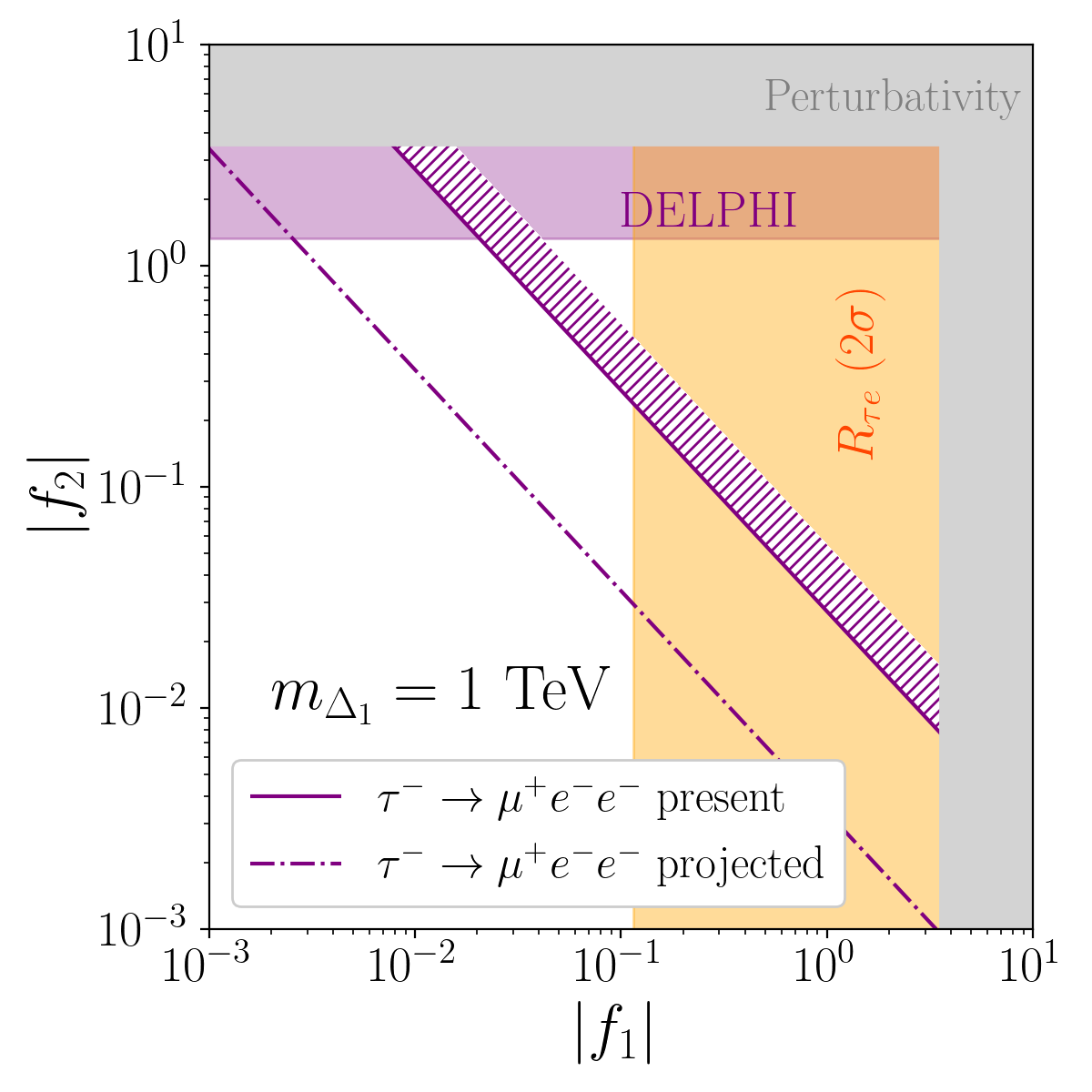
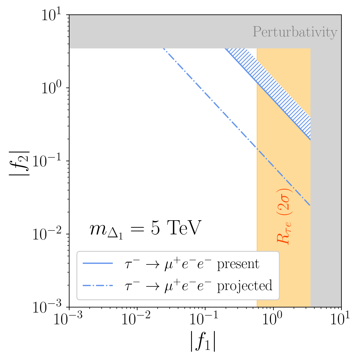
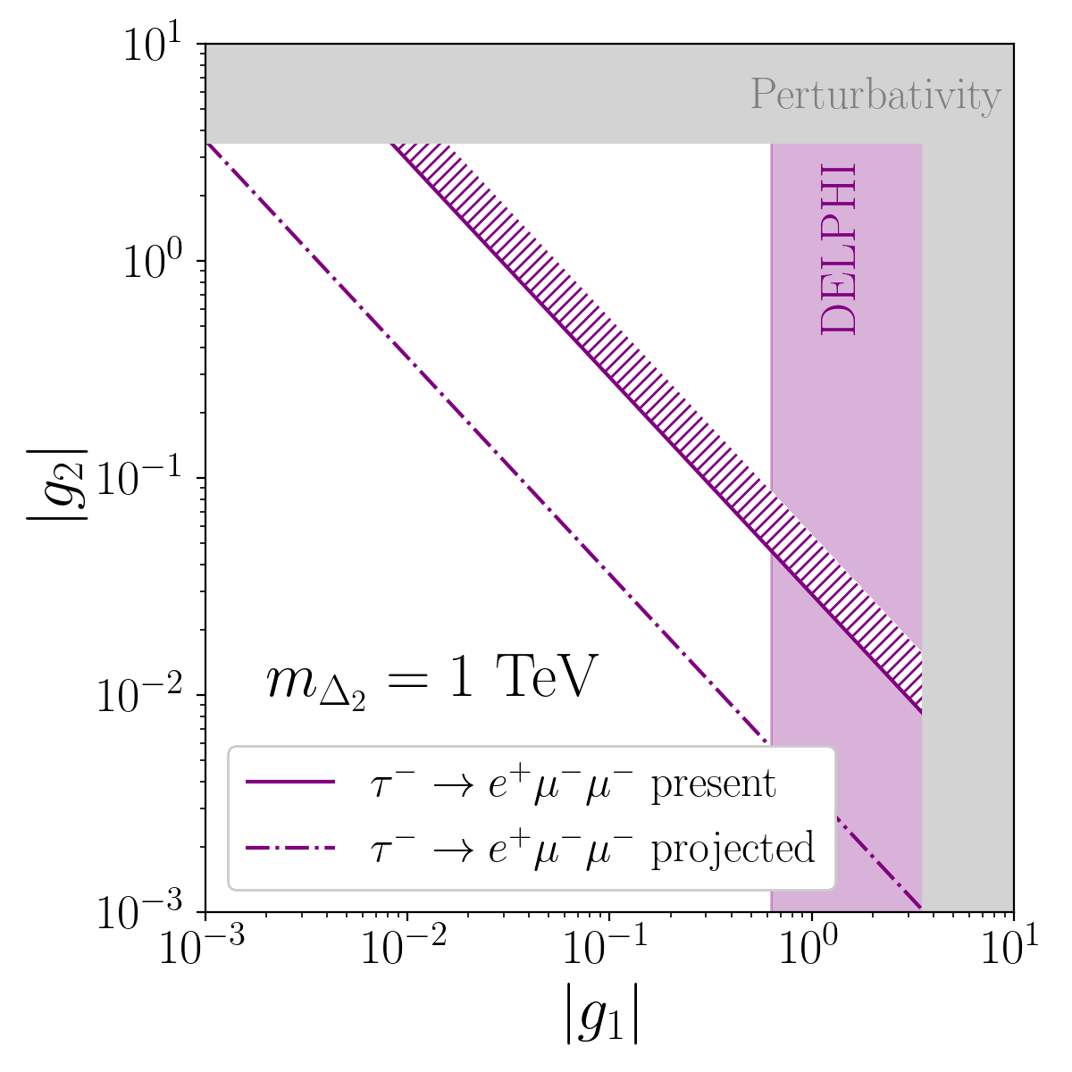
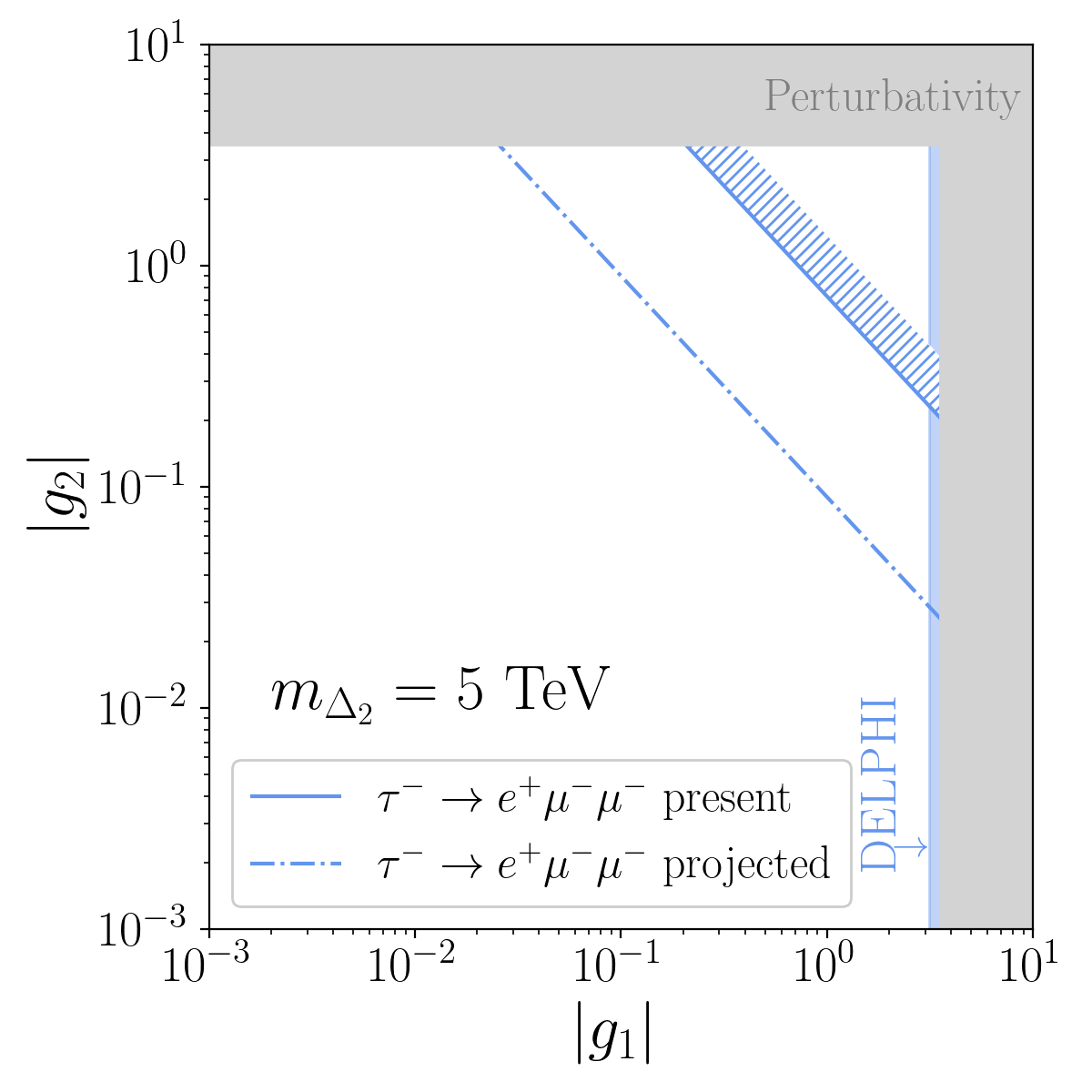
Figure 3: An overview of the electroweak triplet scalar parameter space. The present constraint on cLFV tau decays rules out the parameter space bounded by solid lines, in the direction of the hashing. The reach of Belle II is indicated by dot-dashed lines, i.e. observation of the decay $\tau^{-}\to\mu^{+}e^{-}e^{-}$ ($\tau^{-}\to e^{+}\mu^{-}\mu^{-}$) would be compatible with parameter space in the upper-right in the $|f_{1}|$-$|f_{2}|$ ($|g_{1}|$-$|g_{2}|$) plane above this line. The grey-shaded region is ruled-out by perturbativity of the BSM couplings. The shaded region labelled ‘DELPHI’ is ruled-out by the constraints in Eq. (41), and where this is absent the constraint falls outside the perturbative regime. For the lepton universality ratios double ratios $R_{\ell_{i}\ell_{j}}$ of leptonic $\tau$ decays, the shaded region is the constraint derived when theory is required to match experiment at the $2\sigma$ level, as labelled. For $\Delta_{2}$ in the lower row, these constraints are not shown because they are weaker than those from DELPHI.

III.2 $T=2$ triplet model

Taking the electroweak triplet scalar with lepton triality $T=2$, the Yukawa coupling Lagrangian for $\Delta_{2}$ is

$$\mathcal{L}_{\Delta_{2}}=\frac{1}{2}\left(2g_{1}\overline{L_{3}^{c}}\,i\sigma_{2}\mathbf{\Delta}_{2}\,L_{1}+g_{2}\overline{L_{2}^{c}}\,i\sigma_{2}\mathbf{\Delta}_{2}\,L_{2}\right)+\mathrm{h.c.}$$ (33)

with real and positive Yukawa couplings $g_{1,2}$. These expand out to give Eq. (28) with the substitution $\mu\to e$ for the $g_{1}$ term, and Eq. (29) with $e\to\mu$ for the $g_{2}$ term:

$$\overline{L_{3}^{c}}\ i\sigma_{2}\mathbf{\Delta}_{2}\,L_{1} =-\overline{(\tau_{L})^{c}}\,e_{L}\,\Delta_{2}^{++}-\frac{1}{\sqrt{2}}\left[\overline{(\tau_{L})^{c}}\,\nu_{eL}+\overline{(\nu_{\tau L})^{c}}\,e_{L}\right]\Delta_{2}^{+}+\overline{(\nu_{\tau L})^{c}}\,\nu_{eL}\,\Delta_{2}^{0},$$ (34)

$$\overline{L_{2}^{c}}\ i\sigma_{2}\mathbf{\Delta}_{2}\,L_{2} =-\overline{(\mu_{L})^{c}}\,\mu_{L}\,\Delta_{2}^{++}-\sqrt{2}\,\overline{(\mu_{L})^{c}}\,\nu_{\mu L}\,\Delta_{2}^{+}+\overline{(\nu_{\mu L})^{c}}\,\nu_{\mu L}\,\Delta_{2}^{0}.$$ (35)

The Wilson coefficient

$$C^{VLL}_{ee,2321} =\frac{g_{1}g_{2}}{4m_{\Delta_{2}}^{2}}$$ (36)

parametrises the strength of the decays $\tau^{\pm}\to\mu^{\pm}\mu^{\pm}e^{\mp}$, with the branching ratio being

$$\mathrm{BR}(\tau^{\pm}\to\mu^{\pm}\mu^{\pm}e^{\mp}) =\frac{g_{1}^{2}g_{2}^{2}}{64G_{F}^{2}m_{\Delta_{2}}^{4}}\tilde{I}\left(\frac{m_{\mu}^{2}}{m_{\tau}^{2}}\right)\mathrm{BR}(\tau^{-}\to\mu^{-}\bar{\nu}_{\mu}\nu_{\tau}).$$ (37)

As for the $\Delta_{1}$ model, the current constraint from the non-observation of these decays is the same as for the singlet $k_{2}$ case, i.e. Eq. (14) holds with the $m_{k_{2}}$ replaced by $m_{\Delta_{2}}$,

$$\sqrt{|g_{1}g_{2}|}\lesssim 0.17\ \frac{m_{\Delta_{2}}}{\text{TeV}}$$ (38)

and the Belle II mass reach is roughly $59$ TeV. This bound and the Belle II reach are illustrated in the bottom row of Fig. 3.

III.3 Direct searches

As for the singlet cases, there are constraints from direct searches for doubly-charged scalars decaying to a pair of same-sign leptons. A difference between the singlet and triplet models is that the former involve RH leptons, while the latter feature LH leptons. From the published data of Fig. 13 in Ref. [19] we infer lower limits on the masses of the doubly-charged scalars $\Delta_{1,2}^{++}$ given by

$$m_{\Delta_{1}}\geq 0.69\ \text{TeV}\quad\text{and}\quad m_{\Delta_{2}}\geq 0.73\ \text{TeV}$$ (39)

for the case of 50% BR to electrons and muons, respectively, with the final states containing a $\tau$ which is assumed to be unobserved. For a 100% branching ratio to electrons (muons) the lower bounds become

$$m_{\Delta_{1}}\geq 0.77\ \text{TeV}\quad\text{and}\quad m_{\Delta_{2}}\geq 0.85\ \text{TeV}$$ (40)

according to the published data of Fig. 10 in Ref. [19].

III.4 Lepton scattering constraints

As for the singlet cases, the DELPHI experiment [20] places constraints on the doubly-charged scalar mass $m_{\Delta_{1}}$ and coupling constant $f_{2}$ from $e^{+}e^{-}\to e^{+}e^{-}$, and $m_{\Delta_{2}}$ and $g_{1}$ from $e^{+}e^{-}\to\tau^{+}\tau^{-}$. Translating the results in Ref. [21], we obtain the bounds

$$\frac{m_{\Delta_{1}}}{|f_{2}|} \geq 0.75\,\mathrm{TeV}, \frac{m_{\Delta_{2}}}{|g_{1}|} \geq 1.6\,\mathrm{TeV}.$$ (41)

Note that these constraints are very slightly different from the analogous singlet bounds because the opposite chiral structure changes the details of the interference between the SM and triplet-exchange diagrams.

III.5 Leptonic processes involving neutrinos

The electroweak triplet scalars introduce new contributions to leptonic processes with neutrinos. We follow the discussion in Refs. [22, 21, 29] and focus on the most stringent electroweak physics constraints [22, 21], namely lepton flavour universality, neutrino trident and shifts of the Fermi constant and its impact on the weak mixing angle, the $W$ boson mass and CKM unitarity. The latter three do not receive direct contributions at tree level, but are modified indirectly via the shift of the Fermi constant extracted in muon decay, $G_{F,\mu}$.

In particular, the partial width for the decay $\ell_{\alpha}\to\ell_{\beta}\nu_{i}\bar{\nu}_{j}(\gamma)$ in terms of relevant Wilson coefficients is given by [30, 31, 32, 33]

$$\Gamma(\ell_{\alpha}\to\ell_{\beta}\nu_{i}\bar{\nu}_{j}(\gamma))=\frac{G_{F}^{2}m_{\alpha}^{5}}{192\pi^{3}}I\left(\frac{m_{\beta}^{2}}{m_{\alpha}^{2}}\right)R_{W}R_{\gamma}\sum_{i,j}\frac{|C^{VLL}_{\nu e,ij\beta\alpha}|^{2}+|C^{VLR}_{\nu e,ij\beta\alpha}|^{2}}{8G_{F}^{2}},$$ (42)

where the functions $R_{W}$ and $I$ parameterise corrections from finite lepton masses, while $R_{\gamma}$ parametrises the emission of soft photons. The function $I$ is defined in Eq. (12) and the other functions are given by

$$R_{W}=1+\frac{3}{5}\frac{m_{\alpha}^{2}}{m_{W}^{2}}+\frac{9}{5}\frac{m_{\beta}^{2}}{m_{W}^{2}},\qquad R_{\gamma}=1+\frac{\alpha(m_{\alpha})}{2\pi}\left(\frac{25}{4}-\pi^{2}\right)$$

$$\quad\text{with}\quad\alpha(m_{\alpha})^{-1}=\alpha^{-1}-\frac{2}{3\pi}\ln\left(\frac{m_{\alpha}}{m_{e}}\right)+\frac{1}{6\pi}.$$ (43)

The SM prediction for the LEFT Wilson coefficients is

$$C^{\rm VLL,SM}_{\nu e,ij\beta\alpha} =-2\sqrt{2}G_{F}\left(-\frac{1}{2}+s^{2}_{w}\right)\delta_{ij}\delta_{\alpha\beta}-2\sqrt{2}G_{F}\delta_{i\alpha}\delta_{j\beta}, C^{\rm VLR,SM}_{\nu e,ij\beta\alpha} =-2\sqrt{2}G_{F}s_{w}^{2}\delta_{ij}\delta_{\alpha\beta}.$$ (44)

The electroweak triplet contributes via the 4-lepton SMEFT operators $O^{ll}$ to $C^{VLL}_{\nu e}$ as described by the LEFT matching conditions in App. B and thus modify the leptonic muon and tau decays.

III.5.1 Lepton flavour universality

The most direct probe is provided by the lepton flavour universality double ratios,

$$R_{\mu e} =\frac{\Gamma(\tau\to\mu+\mathrm{inv})}{\Gamma(\tau\to e+\mathrm{inv})}\frac{\Gamma_{\rm SM}(\tau\to e+\mathrm{inv})}{\Gamma_{\rm SM}(\tau\to\mu+\mathrm{inv})},$$ (45)

$$R_{\tau\mu} =\frac{\Gamma(\tau\to e+\mathrm{inv})}{\Gamma(\mu\to e+\mathrm{inv})}\frac{\Gamma_{\rm SM}(\mu\to e+\mathrm{inv})}{\Gamma_{\rm SM}(\tau\to e+\mathrm{inv})},$$ (46)

$$R_{\tau e} =\frac{\Gamma(\tau\to\mu+\mathrm{inv})}{\Gamma(\mu\to e+\mathrm{inv})}\frac{\Gamma_{\rm SM}(\mu\to e+\mathrm{inv})}{\Gamma_{\rm SM}(\tau\to\mu+\mathrm{inv})},$$ (47)

of which only two are independent. For the triplet $\Delta_{1}$ we find

$$R_{\tau e}=R_{\mu e}=\frac{\left(1-\frac{f_{1}^{2}}{8\sqrt{2}G_{F}m_{\Delta_{1}}^{2}}\right)^{2}}{1+\frac{(f_{1}f_{2})^{2}}{2^{7}G_{F}^{2}m_{\Delta_{1}}^{4}}}\approx 1-\frac{f_{1}^{2}}{4\sqrt{2}G_{F}m_{\Delta_{1}}^{2}},\qquad R_{\tau\mu}=1$$ (48)

and for $\Delta_{2}$

$$R_{\tau\mu}=R_{\mu e}^{-1}=\frac{\left(1-\frac{g_{1}^{2}}{8\sqrt{2}G_{F}m_{\Delta_{2}}^{2}}\right)^{2}}{1+\frac{(g_{1}g_{2})^{2}}{2^{7}G_{F}^{2}m_{\Delta_{2}}^{4}}}\approx 1-\frac{g_{1}^{2}}{4\sqrt{2}G_{F}m_{\Delta_{2}}^{2}},\qquad R_{\tau e}=1,$$ (49)

where we neglected terms quartic in the Yukawa couplings in the approximation.

Using the experimental values in Ref. [34], we find for the double ratios [21]

$$R_{\mu e}=1.0034(32),\hskip 14.22636ptR_{\tau\mu}=1.0022(29),\hskip 14.22636ptR_{\tau e}=1.0056(29).$$ (50)

Each of these is to be compared to the SM prediction of unity. We note that there is a tension with the SM prediction for $R_{\tau e}$ which cannot be alleviated at the central value by the electroweak triplet scalar. Requiring that the model agrees with the values in Eq. (50) to within $2\sigma$, the strongest constraints from these ratios come from $R_{\tau e}$ for $\Delta_{1}$ and $R_{\tau\mu}$ for $\Delta_{2}$. The excluded regions are indicated by the vertical coloured bands in the top row of Fig. 3. The region excluded by $R_{\tau\mu}$ is not shown in the bottom row because $|g_{1}|$ is more strongly constrained by the DELPHI measurement.

III.5.2 Trident process

The singly-charged scalar $\Delta_{2}^{+}$ contributes at tree-level via the $g_{2}$ Yukawa interaction to the trident process $\nu_{\mu}N\to\nu_{\mu}\mu^{+}\mu^{-}N$, where $N$ represents a nucleon. This is parameterised by the Wilson coefficient

$$C^{\rm VLL,NP}_{\nu e,2222}=\frac{g_{2}^{2}}{4m_{\Delta_{2}}^{2}},$$ (51)

which gives the ratio of the modified cross section $\sigma$ to the SM cross section $\sigma_{\text{SM}}$ to be

$$\frac{\sigma}{\sigma_{\text{SM}}}=\frac{(1+4\sin^{2}\theta_{w}-C^{\rm VLL,NP}_{\nu e,2222}/(\sqrt{2}G_{F}))^{2}+(1-C^{\rm VLL,NP}_{\nu e,2222}/(\sqrt{2}G_{F}))^{2}}{(1+4\sin^{2}\theta_{w})^{2}+1}.$$ (52)

As the Wilson coefficient $C^{\rm VLL,NP}_{e\nu,2222}$ is strictly positive, the electroweak triplet contribution reduces the ratio to be less than one.

The CHARM-II [35], CCFR [36] and NuTeV [37] experiments have measured this ratio obtaining $1.58\pm 0.64$, $0.82\pm 0.28$ and $0.72^{+1.73}_{-0.72}$, respectively. In order to estimate how neutrino trident production $\nu_{\mu}N\to\nu_{\mu}\mu^{+}\mu^{-}N$ constrains the electroweak triplet scalar $\Delta_{2}$, we combine the experimental measurements to obtain $0.94\pm 0.25$, which constrains

$$-0.15\leq\frac{C^{\rm VLL,NP}_{\nu e,2222}}{\sqrt{2}G_{F}}\leq 0.28\qquad\implies\qquad|g_{2}|\lesssim 4.3\,\frac{m_{\Delta_{2}}}{\text{TeV}}.$$ (53)

This may be compared with the bound in Eq. (38). Numerically it is a weak constraint, with the upper bound on $g_{2}$ in the non-perturbative regime and thus moot. However, it is worth noting that the constraint is purely on $g_{2}$ rather than the product $g_{1}g_{2}$, and so in principle the trident process provides a complementary constraint.

As this constraint is rather weak in this model (and also orthogonal to the main discussion of cLFV leptonic $\tau$ decays) we do not discuss the sensitivity of neutrino trident processes at DUNE. DUNE is able to measure other trident processes, including lepton-flavour-violating neutrino trident processes. See Refs. [38, 39] for a detailed discussion of neutrino tridents at DUNE.

III.5.3 Fermi constant

Input	Value
$m_{Z}$	$91.1876(21)$ GeV
$G_{F,\mu}$	$1.1663787(6)\times 10^{-5}$ GeV-2
$\alpha^{-1}$	137.035999180(10)

Table 2: Input parameters for electroweak observables, taken from Ref. [34].

These models generate new contributions to muon decay, which is used to determine the Fermi constant $G_{F}$. We denote the Fermi constant determined through muon decay $G_{F,\mu}$. Using the input parameters for the SM electroweak observables listed in Table 2, these contributions introduce a shift in $G_{F,\mu}$,

$$G_{F,\mu}^{2}=\frac{1}{8}\sum_{i,j}\left(|C^{VLL}_{\nu e,ij12}|^{2}+|C^{VLR}_{\nu e,ij12}|^{2}\right),$$ (54)

in contrast to the SM value $G_{F,0}=(\sqrt{2}v^{2})^{-1/2}$. Here $v$ is the vacuum expectation value (VEV) of the Higgs field $\left\langle H\right\rangle=v/\sqrt{2}$. We define $G_{F,0}=G_{F,\mu}(1+\delta G_{F})$, and for $\Delta_{1}$ and $\Delta_{2}$ we find that

$$\delta G_{F} =\begin{cases}-\frac{f_{1}^{2}f_{2}^{2}}{1024G_{F,\mu}^{2}m_{\Delta_{1}}^{4}}&\mathrm{for}\;\Delta_{1},\\[8.61108pt] -\frac{g_{1}^{2}g_{2}^{2}}{1024G_{F,\mu}^{2}m_{\Delta_{2}}^{4}}&\mathrm{for}\;\Delta_{2}.\end{cases}$$ (55)

As the correction to the Fermi constant only occurs at quartic order in the Yukawa couplings, we do not expect strong constraints from $\delta G_{F}$.

Several measurements are sensitive to the Fermi constant and thus provide constraints on $\delta G_{F}$. Here we consider the weak mixing angle, the $W$ boson mass and CKM unitarity as a subset of these measurements. For each of these, we use the tree-level SM expression to determine how the shift in $G_{F}$ affects the observable, and then derive a constraint on the shift $\delta G_{F}$ the electroweak fit from Ref. [40] (which includes loop-level SM corrections). This fit provides SM predictions for the different observables (without including the measurements) which are then compared to the experimental measurements to obtain constraints on $\delta G_{F}$.

The effective leptonic weak mixing angle does not receive direct corrections at tree-level because the $Z$ boson couplings to leptons are not modified. Therefore, we find

$$\bar{s}_{\ell}^{2} =s_{w,0}^{2}\left(1-\frac{1-s_{w,0}^{2}}{1-2s_{w,0}^{2}}\delta G_{F}\right),$$ (56)

which has been obtained from the tree-level SM prediction of the weak mixing angle

$$s_{w,0}^{2}=\frac{1}{2}\left(1-\sqrt{1-\frac{4\pi\alpha}{\sqrt{2}G_{F}m_{Z}^{2}}}\right).$$ (57)

Contrasting this with the experimental result $\bar{s}_{\ell,\rm exp}^{2}(\mathrm{LEP})=0.23153(4)$ [41] with the loop-corrected SM prediction for the weak mixing angle based on the fit in [40], $\bar{s}_{\ell,\rm SM}^{2}=0.231534(41)$, results in

$$\delta G_{F}=12(170)\times 10^{-6}.$$ (58)

A shift in the Fermi constant also translates to a shift in the $W$ boson mass

$$m_{W}^{2}=m_{W,0}^{2}\left(1+\frac{s_{w,0}^{2}}{1-2s_{w,0}^{2}}\delta G_{F}\right)$$ (59)

which has been derived from the tree-level SM prediction

$$m_{W,0}=m_{Z}\sqrt{1-s_{w,0}^{2}}.$$ (60)

A comparison of the experimental global fit to the $W$ boson mass excluding the new CDF measurement $m_{W,\rm exp}=80.377(12)$ [34] [and a combination of all Tevatron measurements by themselves $m_{W,\rm Tevatron}=$80.4274(89) [42]] with the SM prediction $m_{W}=80.3545(42)$ GeV [40] results in

$$\delta G_{F}=0.00130(73)\,[0.00421(57)].$$ (61)

A shift in the Fermi constant also leads to an apparent violation of CKM unitarity. We find for the unitarity relation of the first row CKM matrix elements that

$$\sum_{\beta}|V_{u\beta}|^{2}=1+2\delta G_{F}.$$ (62)

The global fit in Ref. [34] requires $\sum_{\beta}|V_{u\beta}|^{2}=0.9985\pm 0.0007$. If we conservatively demand consistency at $3\sigma$ (to include the SM prediction), we find

$$\delta G_{F}=-0.00075(35).$$ (63)

Note that the different observables are in tension with each other: the leptonic weak mixing angle prefers no correction to $\delta G_{F}$, the $W$ boson mass indicates a positive $\delta G_{F}$, and CKM unitarity negative $\delta G_{F}$. As $\delta G_{F}$ in the electroweak triplet model is proportional to the fourth power of Yukawa couplings, none of the observables constraining $\delta G_{F}$ provide a competitive constraint. Even the sensitivity of the leptonic weak mixing angle (which probes $\delta G_{F}$ at the level of $10^{-4}$) is only sensitive to scales $m_{\Delta_{T}}\lesssim 0.50$ TeV for Yukawa couplings of order unity, which is already excluded by direct searches at the LHC (see Sec. III.3).

III.6 Other observables

As discussed for the electroweak singlet scalar, there are new contributions to leptonic Higgs and $Z$ boson decays and the anomalous magnetic moment [22, 21]. These are too small to have any measurable phenomenological implications.

IV Phase space

In the caption of Table 1, we alluded to upper limits placed by experiment on cLFV leptonic $\tau$ decays depending on the assumed distribution of signal events. The limits quoted in this table are extracted by the experimental collaborations assuming that the leptons from the $\tau$-decay follow a phase space distribution, i.e. no kinematic dependence in the matrix element. The model-discriminating power of three-body phase space in tau decays has been studied, for example, in Refs. [43, 44, 45, 46].

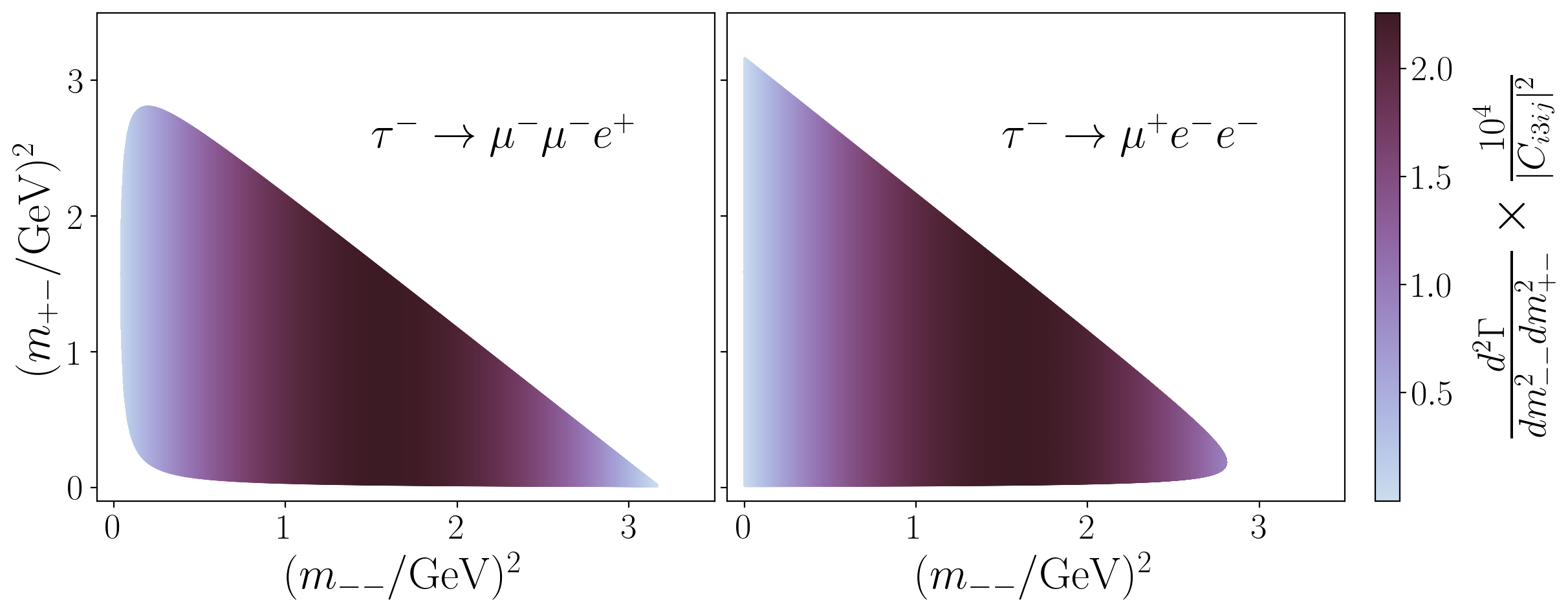
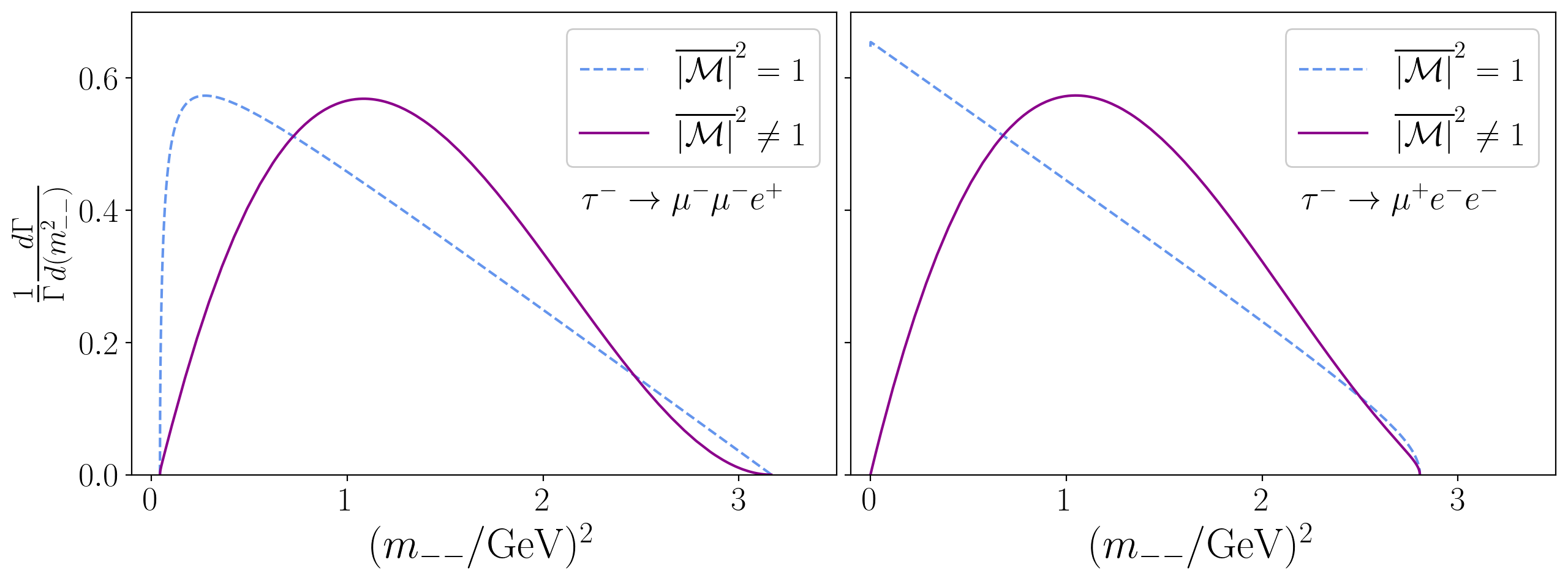
Figure 4: A study of key cLFV tau decay phase space. The top row shows Dalitz plots for the two key decay processes $\tau^{-}\to\mu^{-}\mu^{-}e^{+}$ (left) and $\tau^{-}\to\mu^{+}e^{-}e^{-}$ (right) assuming the dominant contribution is via the left or right-handed vector operator $C_{i3ij}$, as appears in Eq. (64). The bottom row shows the integrated differential distributions with respect to the observable $m_{--}^{2}$, illustrating the difference between the kinematic distribution of this model ($\overline{|{\mathcal{M}}|}^{2}\neq 1$ as per Eq. (64), solid purple line) and the phase space distribution ($\overline{|{\mathcal{M}}|}^{2}=1$, blue dashed line).

In the both the electroweak singlet and triplet models, the differential decay rate for $\tau^{-}\to\ell_{i}^{-}{\ell}_{i}^{-}\ell_{j}^{+}$ is given by

$$\frac{d^{2}\Gamma(\tau^{-}\to\ell_{i}^{-}{\ell}_{i}^{-}\ell_{j}^{+})}{dm_{--}^{2}\,dm_{+-}^{2}} =\frac{1}{256\pi^{3}m_{\tau}^{3}}\overline{|\mathcal{M}|}^{2}=\frac{|C_{i3ij}|^{2}}{64\pi^{3}m_{\tau}^{3}}(m_{--}^{2}-2m_{\ell_{i}}^{2})(m_{\tau}^{2}+m_{\ell_{j}}^{2}-m_{--}^{2}),$$ (64)

where $m_{--}^{2}=(p_{\ell_{i}}+p_{\ell^{\prime}_{i}})^{2}$ is the invariant mass of the system of two same-sign leptons in the final state, $m_{+-}^{2}=(p_{\ell_{i}}+p_{\ell_{j}})^{2}$ is that of two oppositely charged final state leptons, and $\overline{|\mathcal{M}|}^{2}$ is the spin-averaged matrix element for the process. The squared Wilson coefficient is given by $|C_{i3ij}|^{2}=|C^{\rm VRR}_{ee,i3ij}|^{2}$ in the electroweak singlet models and by $|C_{i3ij}|^{2}=|C^{VLL}_{ee,i3ij}|^{2}$ in the electroweak triplet models. Thus all models feature the same distributions for the differential decay rates. A so-called phase space distribution for the differential decay rate discussed in this section corresponds to setting $\overline{|\mathcal{M}|}^{2}=1$.

From Eq. (64) there is a flat distribution in $m^{2}_{+-}$ and a peak in $m^{2}_{--}$ at $m^{2}_{--}=\frac{1}{2}(2m_{\ell_{i}}^{2}+m_{\ell_{j}}+m_{\tau}^{2})\approx\frac{1}{2}m^{2}_{\tau}$, where the latter approximation corresponds to neglecting the mass of leptons in the final state. This is illustrated by the Dalitz plots in the top row of Figure 4. The structure of these Dalitz distributions is characteristic of models in which the dominant BSM contribution to these processes is via a RH or LH vector operator, respectively. Ultimately if these decays are detected with significant multiplicity, an analysis of the three-body phase space could discriminate between different BSM explanations [43].

In the bottom row of Figure 4 we illustrate the corresponding $\frac{d\Gamma(\tau^{-}\to\ell_{i}^{-}{\ell}_{i}^{-}\ell_{j}^{+})}{dm_{--}^{2}}$ distribution (solid purple), comparing it to a phase space distribution (dashed blue). Integration over $m_{+-}^{2}$ results in a factor

$$m_{+-,\rm max}^{2}-m_{+-,\rm min}^{2}=\frac{\lambda^{1/2}(m_{\tau}^{2},m_{--}^{2},m_{\ell_{j}}^{2})\lambda^{1/2}(m_{--}^{2},m_{\ell_{i}}^{2},m_{\ell_{i}}^{2})}{m_{--}},$$ (65)

where $\lambda^{1/2}$ is the square-root of the Källén function, and the invariant mass $m_{--}^{2}$ takes values in the range $4m_{\ell_{i}}^{2}<m_{--}^{2}<(m_{\tau}-m_{\ell_{j}})^{2}$. Integration of the differential decay width results in the expressions shown in Eqs. (6) and (11).

Even with non-observation in these channels, the expected number of events in different kinematic regions is shown in Figure 4 to vary model-dependently (this was also emphasised in Refs. [43, 44, 45, 46], although they did not study these two decay channels). As such, an exclusion should be weighted accordingly to provide the most accurate measure of the present and projected constraint – although it is not feasible for an experimental collaboration to present constraints on each individual model or even at the EFT level, where interference effects would also need to be considered. Without access to internal Belle/ Belle II information, one cannot easily recast the branching-ratio limits to a specific model, and so we still adopt the values derived using the assumption of a phase space distribution (Table 1). In the absence of events, recasting the limits based on the phase space distribution requires the detection efficiency as a function of the invariant masses $m_{--}^{2}$ and $m_{+-}^{2}$.

V Neutrino masses

So far, we have mainly focused on the charged-lepton sector. In this section we turn to neutrino masses and discuss a few possible scenarios how non-zero neutrino masses may be incorporated into these models.

The most straightforward way to generate non-zero neutrino masses in both the electroweak singlet and triplet models is by introducing three RH sterile neutrinos with similar $Z_{3}$ triality charges. The first (second) [third] generation of sterile neutrinos has charge $T=1$ ($2$) [$3$]. These charges correspond to the transformations

$$\nu_{R}\to\omega^{T}\nu_{R}$$ (66)

where $\nu_{R}$ are the RH neutrinos. Given these assignments, the neutrino Yukawa and mass terms in the Lagrangian are

$$-\mathcal{L}\supset y_{\nu i}\bar{L}_{i}\nu_{Ri}\tilde{H}+\frac{1}{2}M_{ij}\overline{(\nu_{Ri})^{c}}\,\nu_{Rj}+\mathrm{h.c.},$$ (67)

where $i,j=1,2,3$ with repeated indices summed, $\tilde{H}=i\tau_{2}H^{*}$, $y_{\nu i}$ denotes the neutrino Yukawa couplings, and $M$ is the RH neutrino Majorana mass matrix. The neutrino Dirac mass matrix is diagonal. With exact triality, the RH neutrino Majorana mass matrix is constrained to the form

$$M=\left(\begin{array}[]{ccc}0&M_{12}&0\\ M_{12}&0&0\\ 0&0&M_{33}\end{array}\right).$$ (71)

This is incompatible with the neutrino oscillation data, given that we also have a diagonal neutrino Dirac mass matrix. Therefore lepton triality must be broken. This breaking could be achieved by via explicit soft-breaking operators, which then generate the remaining entries of the RH neutrino mass matrix. Alternatively, it can be achieved by introducing a SM singlet complex scalar $S$ with $T=1$ (so that $S\to\omega S$ and $S^{*}\to\omega^{2}S^{*}$) which leads to the additional triality-preserving Yukawa coupling terms

$$\mathcal{L} \supset\frac{1}{2}\left[x_{11}\overline{(\nu_{R1})^{c}}\,\nu_{R1}+x_{23}\left(\overline{(\nu_{R2})^{c}}\,\nu_{R3}+\overline{(\nu_{R3})^{c}}\,\nu_{R2}\right)\right]S$$

$$+\frac{1}{2}\left[x_{22}\overline{(\nu_{R2})^{c}}\,\nu_{R2}+x_{13}\left(\overline{(\nu_{R1})^{c}}\,\nu_{R3}+\overline{(\nu_{R3})^{c}}\,\nu_{R1}\right)\right]S^{*}+\mathrm{h.c.}\;.$$ (72)

Triality is then spontaneously broken by a nonzero VEV for $S$, and the zero entries in Eq. (71) are now all generated. A diagonal neutrino Dirac mass matrix together with a general RH neutrino Majorana mass matrix is able to accommodate the neutrino oscillation data.

Adopting the type-I seesaw mechanism requires the VEV-generated triality-breaking terms to be of a high scale, not dissimilar to $M_{12}$ and $M_{33}$. Note that the $S$ and $S^{*}$ Yukawa terms combine to explicitly break lepton-number conservation. Lepton number is also explicitly broken by a cubic $(aS^{3}+\mathrm{h.c.})$ triality-preserving term in the scalar potential, which means that the phase of $S$ is not a Goldstone boson. Neutrino masses can equally well generated using the type-III seesaw mechanism [47] with electroweak triplet fermions instead of electroweak singlet fermions.

As was mentioned in the introduction, lepton triality is motivated by discrete flavour symmetries, which break the flavour group to a $Z_{3}$ subgroup in the charged lepton sector and to a $Z_{2}$ subgroup in the neutrino sector. The misalignment between the two sectors explains the leptonic mixing matrix with the prime example for this construction being the $A_{4}$ flavour group. Assuming that the additional BSM physics related to the flavour symmetry is sufficiently decoupled, the $A_{4}$ flavour symmetry models for neutrino masses mentioned in the introduction (Refs. [3, 4, 5, 6, 7, 8, 9, 10, 11]) also yield the phenomenology of charged leptons discussed in this paper.

Aside from triality, the electroweak triplet scalar is that of the type-II seesaw mechanism. A nonzero VEV for $\Delta_{T}^{0}$ would therefore contribute some direct Majorana mass terms for the light neutrinos. The VEV is naturally suppressed because the cubic Higgs coupling $H^{T}i\sigma_{2}\mathbf{\Delta}_{T}^{\dagger}H$ softly breaks lepton triality. Similarly, the electroweak singlet scalar features in the Zee-Babu model [48, 49]. See [14, 50, 51] for recent phenomenological studies.

As it becomes evident from the discussion of the seesaw mechanisms, lepton triality has to be broken to achieve the observed leptonic mixing pattern [52, 53]. This can also be seen more generally by considering the Weinberg operator [54],

$$\mathcal{L}_{5}=-\frac{\kappa_{ij}}{4}(L_{i}H)^{T}C(L_{j}H)+\mathrm{h.c.}\;,$$ (73)

where the SU(2) indices are contracted within each pair of parentheses. Lepton triality constrains the Wilson coefficient to take the form

$$\kappa=\begin{pmatrix}0&\kappa_{12}&0\\ \kappa_{12}&0&0\\ 0&0&\kappa_{33}\end{pmatrix}\;.$$ (74)

Like for the case of the seesaw mechanism, lepton triality has to be broken to explain the observed lepton mixing matrix which may be achieved by introducing a SM singlet complex scalar $S$ with $T=1$ and an effective dimension-6 operators $S^{(*)}(L_{i}H)^{T}C(L_{j}H)$. A similar argument can be made for Dirac neutrinos, because the Yukawa interaction $\bar{L}_{i}\nu_{Rj}\tilde{H}$ and thus the neutrino Dirac mass term contain at most 3 non-zero entries for the lepton triality charges defined in Eq. (2) irrespective of the lepton triality charges of the RH neutrinos.

VI Conclusions

Charged lepton flavour-violating decays and other related processes are an important probe of physics beyond the standard model. The discovery of neutrino flavour oscillations implies that such processes must occur at some level, but for them to be observable in practice physics in addition to that responsible for neutrino mass generation must exist. Importantly, significant advances in the search for flavour-violating $\tau$ decays will be made by the Belle II experiment over the next few years, thus opening a new discovery window. In this paper we presented very simple models based on the flavour symmetry structure of lepton triality that feature the decays $\tau^{\pm}\to\mu^{\pm}\mu^{\pm}e^{\mp}$ and $\tau^{\pm}\to e^{\pm}e^{\pm}\mu^{\mp}$ as the dominant signals of BSM physics. These decays are driven by the tree-level exchange of doubly-charged scalars shown Fig. 1. As illustrated in Figs. 2 and 3, the eventual Belle II sensitivity to these processes will see significantly more parameter space explored compared to the present situation, either discovering evidence of new physics or further constraining the possibilities.

These models are simple examples of minimal SM extensions that single out the $\tau$ sector for the dominant phenomenological signatures. The fact that it proves so easy to do this highlights the importance and relevance of the on-going experimental searches. We expect that our minimal models may be embedded in more complete theories of flavour symmetry and, beyond this, that quite different schemes could also be constructed to achieve a similar purpose.

Appendix A SMEFT

In addition to the renormalisable part of the Lagrangian we introduce dimension-6 SMEFT operators. We are particularly interested in operators which violate lepton flavour and are consistent with the $Z_{3}$ symmetry. The only relevant operators in the Warsaw basis [55] are the 4-lepton operators

$$\mathcal{L}_{6} =C^{ll}(\bar{L}\gamma_{\mu}L)(\bar{L}\gamma^{\mu}L)+C^{ee}(\bar{e}_{R}\gamma_{\mu}e_{R})(\bar{e}_{R}\gamma^{\mu}e_{R})+C^{le}(\bar{L}\gamma_{\mu}L)(\bar{e}_{R}\gamma^{\mu}e_{R}),$$ (75)

where we do not explicitly specify the flavour indices. In case flavour indices are important, they are written as subscripts in the order of the fermion flavours in the operators, e.g. $C^{ll}_{abcd}$ is the Wilson coefficient of operator $(\bar{L}_{a}\gamma_{\mu}L_{b})(\bar{L}_{c}\gamma^{\mu}L_{d})$.

The electroweak singlet models lead to

$$C^{ee}_{3322} =\frac{|f_{1}|^{2}}{2m_{k_{1}}^{2}} C^{ee}_{1111} =\frac{|f_{2}|^{2}}{8m_{k_{1}}^{2}} C^{ee}_{1312} =C^{ee*}_{3121}=\frac{f_{1}f_{2}^{*}}{4m_{k_{1}}^{2}}$$ (76)

$$C^{ee}_{3311} =\frac{|g_{1}|^{2}}{2m_{k_{2}}^{2}} C^{ee}_{2222} =\frac{|g_{2}|^{2}}{8m_{k_{2}}^{2}} C^{ee}_{2321} =C^{ee*}_{3212}=\frac{g_{1}g_{2}^{*}}{4m_{k_{2}}^{2}},$$ (77)

where we removed equivalent Wilson coefficients and only keep one of the equivalent flavour combinations. For the electroweak triplet models we find

$$C^{ll}_{3322} =C^{ll}_{3223}=\frac{|f_{1}|^{2}}{4m_{\Delta_{1}}^{2}} C^{ll}_{1111} =\frac{|f_{2}|^{2}}{8m_{\Delta_{1}}^{2}} C^{ll}_{1312} =C^{ll*}_{3121}=\frac{f_{1}f_{2}^{*}}{4m_{\Delta_{1}}^{2}}$$ (78)

$$C^{ll}_{3311} =C^{ll}_{3113}=\frac{|g_{1}|^{2}}{4m_{\Delta_{2}}^{2}} C^{ll}_{2222} =\frac{|g_{2}|^{2}}{8m_{\Delta_{2}}^{2}} C^{ll}_{2321} =C^{ll*}_{3212}=\frac{g_{1}g_{2}^{*}}{4m_{\Delta_{2}}^{2}}.$$ (79)

As lepton triality protects the flavour structure of the operators, no operator violating lepton triality is generated by renormalisation group corrections. Thus in this analysis we neglect renormalisation group corrections.

Appendix B LEFT

As the $Z_{3}$ symmetry only allows lepton-flavour-violating 4-fermion operators at dimension-6 in SMEFT, we consider only leptonic 4-fermion interactions in LEFT [56]:

$$\mathcal{L} =C^{VLL}_{ee}(\bar{e}\gamma^{\mu}e_{L})(\bar{e}\gamma_{\mu}e_{L})+C^{VRR}_{ee}(\bar{e}\gamma^{\mu}e_{R})(\bar{e}\gamma_{\mu}e_{R})+C^{VLR}_{ee}(\bar{e}\gamma^{\mu}e_{L})(\bar{e}\gamma_{\mu}e_{R})$$ (80)

$$+C^{VLL}_{\nu e}(\bar{\nu}\gamma^{\mu}\nu_{L})(\bar{e}\gamma_{\mu}e_{L})+C^{VLR}_{\nu e}(\bar{\nu}\gamma^{\mu}\nu_{L})(\bar{e}\gamma_{\mu}e_{R}).$$

Similarly to the SMEFT operators, we do not explicitly specify the flavour indices, unless needed. In case flavour indices are important, they are written as subscripts in the order of the fermion flavours in the operator, e.g. $C^{VLL}_{ee,abcd}$ is the Wilson coefficient of $(\bar{e}_{a}\gamma^{\mu}P_{L}e_{b})(\bar{e}_{c}\gamma_{\mu}P_{L}e_{d})$. We do not include the 4-neutrino operator, because it is not relevant for the discussion of the phenomenology. Other lepton-flavour-violating Wilson coefficients are strongly suppressed by the unitarity of the PMNS mixing matrix and are neglected.

The matching to LEFT operators is given by [56]

$$C^{VLL}_{ee,ijkl} =C^{ll}_{ijkl}-\frac{g_{Z}^{2}}{4m_{Z}^{2}}[Z_{e_{L}}]_{ij}[Z_{e_{L}}]_{kl}-\frac{g_{Z}^{2}}{4m_{Z}^{2}}[Z_{e_{L}}]_{il}[Z_{e_{L}}]_{kj},$$ (81)

$$C^{VRR}_{ee,ijkl} =C^{ee}_{ijkl}-\frac{g_{Z}^{2}}{4m_{Z}^{2}}[Z_{e_{R}}]_{ij}[Z_{e_{R}}]_{kl}-\frac{g_{Z}^{2}}{4m_{Z}^{2}}[Z_{e_{R}}]_{il}[Z_{e_{R}}]_{kj},$$ (82)

$$C^{VLR}_{ee,ijkl} =C^{le}_{ijkl}-\frac{g_{Z}^{2}}{m_{Z}^{2}}[Z_{e_{R}}]_{ij}[Z_{e_{R}}]_{kl},$$ (83)

$$C^{VLL}_{\nu e,ijkl} =C^{ll}_{ijkl}+C^{ll}_{klij}-\frac{g^{2}}{2m_{W}^{2}}[W_{l}]_{il}[W_{l}]_{jk}^{*}-\frac{g_{Z}^{2}}{m_{Z}^{2}}[Z_{\nu}]_{ij}[Z_{e_{L}}]_{kl},$$ (84)

$$C^{VLR}_{\nu e,ijkl} =C^{le}_{ijkl}-\frac{g_{Z}^{2}}{m_{Z}^{2}}[Z_{\nu}]_{ij}[Z_{e_{R}}]_{kl},$$ (85)

with the SM contributions via $W$ and $Z$ boson exchange

$$[Z_{\nu}]_{pr} =\frac{1}{2}\delta_{pr}, [Z_{e_{L}}]_{pr} =\left(-\frac{1}{2}+s_{w}^{2}\right)\delta_{pr}, [Z_{e_{R}}]_{pr} =s_{w}^{2}\delta_{pr}, [W_{l}]_{pr} =\delta_{pr}.$$ (86)

The Fermi constant in the SM is given by $2\sqrt{2}G_{F}=\frac{g^{2}}{2m_{W}^{2}}=\frac{g_{Z}^{2}}{2m_{Z}^{2}}$ and thus Eqs. (84,85) result in the SM contribution shown in Eq. (44). Renormalisation group corrections are dominated by QED running and thus generally small, so we neglect them throughout this analysis.

References

- Hayasaka et al. [2010] K. Hayasaka et al., Search for Lepton Flavor Violating Tau Decays into Three Leptons with 719 Million Produced Tau+Tau- Pairs, Phys. Lett. B 687, 139 (2010), arXiv:1001.3221 [hep-ex] .
- Banerjee et al. [2022] S. Banerjee et al., Snowmass 2021 White Paper: Charged lepton flavor violation in the tau sector (2022), arXiv:2203.14919 [hep-ph] .
- Altarelli and Feruglio [2006] G. Altarelli and F. Feruglio, Tri-bimaximal neutrino mixing, A(4) and the modular symmetry, Nucl. Phys. B 741, 215 (2006), arXiv:hep-ph/0512103 .
- He et al. [2006] X.-G. He, Y.-Y. Keum, and R. R. Volkas, A(4) flavor symmetry breaking scheme for understanding quark and neutrino mixing angles, JHEP 04, 039, arXiv:hep-ph/0601001 .
- Ma [2010] E. Ma, Quark and Lepton Flavor Triality, Phys. Rev. D 82, 037301 (2010), arXiv:1006.3524 [hep-ph] .
- de Adelhart Toorop et al. [2011a] R. de Adelhart Toorop, F. Bazzocchi, L. Merlo, and A. Paris, Constraining Flavour Symmetries At The EW Scale I: The A4 Higgs Potential, JHEP 03, 035, [Erratum: JHEP 01, 098 (2013)], arXiv:1012.1791 [hep-ph] .
- de Adelhart Toorop et al. [2011b] R. de Adelhart Toorop, F. Bazzocchi, L. Merlo, and A. Paris, Constraining Flavour Symmetries At The EW Scale II: The Fermion Processes, JHEP 03, 040, arXiv:1012.2091 [hep-ph] .
- Cao et al. [2011] Q.-H. Cao, A. Damanik, E. Ma, and D. Wegman, Probing Lepton Flavor Triality with Higgs Boson Decay, Phys. Rev. D 83, 093012 (2011), arXiv:1103.0008 [hep-ph] .
- Holthausen et al. [2013] M. Holthausen, M. Lindner, and M. A. Schmidt, Lepton flavor at the electroweak scale: A complete model, Phys. Rev. D 87, 033006 (2013), arXiv:1211.5143 [hep-ph] .
- Pascoli and Zhou [2016] S. Pascoli and Y.-L. Zhou, Flavon-induced connections between lepton flavour mixing and charged lepton flavour violation processes, JHEP 10, 145, arXiv:1607.05599 [hep-ph] .
- Muramatsu et al. [2016] Y. Muramatsu, T. Nomura, and Y. Shimizu, Mass limit for light flavon with residual Z3 symmetry, JHEP 03, 192, arXiv:1601.04788 [hep-ph] .
- Cuypers and Davidson [1998] F. Cuypers and S. Davidson, Bileptons: Present limits and future prospects, Eur. Phys. J. C 2, 503 (1998), arXiv:hep-ph/9609487 .
- Akeroyd et al. [2007] A. G. Akeroyd, M. Aoki, and Y. Okada, Lepton Flavour Violating tau Decays in the Left-Right Symmetric Model, Phys. Rev. D 76, 013004 (2007), arXiv:hep-ph/0610344 .
- Nebot et al. [2008] M. Nebot, J. F. Oliver, D. Palao, and A. Santamaria, Prospects for the Zee-Babu Model at the CERN LHC and low energy experiments, Phys. Rev. D 77, 093013 (2008), arXiv:0711.0483 [hep-ph] .
- Akeroyd et al. [2009] A. G. Akeroyd, M. Aoki, and H. Sugiyama, Lepton Flavour Violating Decays and in the Higgs Triplet Model, Phys. Rev. D 79, 113010 (2009), arXiv:0904.3640 [hep-ph] .
- Heeck [2017] J. Heeck, Interpretation of Lepton Flavor Violation, Phys. Rev. D 95, 015022 (2017), arXiv:1610.07623 [hep-ph] .
- Crivellin et al. [2019] A. Crivellin, M. Ghezzi, L. Panizzi, G. M. Pruna, and A. Signer, Low- and high-energy phenomenology of a doubly charged scalar, Phys. Rev. D 99, 035004 (2019), arXiv:1807.10224 [hep-ph] .
- Bhupal Dev et al. [2018] P. S. Bhupal Dev, R. N. Mohapatra, and Y. Zhang, Probing TeV scale origin of neutrino mass at future lepton colliders via neutral and doubly-charged scalars, Phys. Rev. D 98, 075028 (2018), arXiv:1803.11167 [hep-ph] .
- Aaboud et al. [2018] M. Aaboud et al. (ATLAS), Search for doubly charged Higgs boson production in multi-lepton final states with the ATLAS detector using proton–proton collisions at , Eur. Phys. J. C 78, 199 (2018), arXiv:1710.09748 [hep-ex] .
- Abdallah et al. [2006] J. Abdallah et al. (DELPHI), Measurement and interpretation of fermion-pair production at LEP energies above the Z resonance, Eur. Phys. J. C 45, 589 (2006), arXiv:hep-ex/0512012 .
- Li and Schmidt [2019a] T. Li and M. A. Schmidt, Sensitivity of future lepton colliders and low-energy experiments to charged lepton flavor violation from bileptons, Phys. Rev. D 100, 115007 (2019a), arXiv:1907.06963 [hep-ph] .
- Li and Schmidt [2019b] T. Li and M. A. Schmidt, Sensitivity of future lepton colliders to the search for charged lepton flavor violation, Phys. Rev. D 99, 055038 (2019b), arXiv:1809.07924 [hep-ph] .
- Konetschny and Kummer [1977] W. Konetschny and W. Kummer, Nonconservation of Total Lepton Number with Scalar Bosons, Phys. Lett. B 70, 433 (1977).
- Magg and Wetterich [1980] M. Magg and C. Wetterich, Neutrino Mass Problem and Gauge Hierarchy, Phys. Lett. B 94, 61 (1980).
- Cheng and Li [1980] T. P. Cheng and L.-F. Li, Neutrino Masses, Mixings and Oscillations in SU(2) x U(1) Models of Electroweak Interactions, Phys. Rev. D 22, 2860 (1980).
- Schechter and Valle [1980] J. Schechter and J. W. F. Valle, Neutrino Masses in SU(2) x U(1) Theories, Phys. Rev. D 22, 2227 (1980).
- Du et al. [2022] Y. Du, X.-X. Li, and J.-H. Yu, Neutrino seesaw models at one-loop matching: discrimination by effective operators, JHEP 09, 207, arXiv:2201.04646 [hep-ph] .
- Li et al. [2022] X. Li, D. Zhang, and S. Zhou, One-loop matching of the type-II seesaw model onto the Standard Model effective field theory, JHEP 04, 038, arXiv:2201.05082 [hep-ph] .
- Li et al. [2021] T. Li, M. A. Schmidt, C.-Y. Yao, and M. Yuan, Charged lepton flavor violation in light of the muon magnetic moment anomaly and colliders, Eur. Phys. J. C 81, 811 (2021), arXiv:2104.04494 [hep-ph] .
- Kinoshita and Sirlin [1959] T. Kinoshita and A. Sirlin, Radiative corrections to Fermi interactions, Phys. Rev. 113, 1652 (1959).
- Marciano and Sirlin [1988] W. J. Marciano and A. Sirlin, Electroweak Radiative Corrections to tau Decay, Phys. Rev. Lett. 61, 1815 (1988).
- Fael et al. [2013] M. Fael, L. Mercolli, and M. Passera, W-propagator corrections to and leptonic decays, Phys. Rev. D 88, 093011 (2013), arXiv:1310.1081 [hep-ph] .
- Ferroglia et al. [2013] A. Ferroglia, C. Greub, A. Sirlin, and Z. Zhang, Contributions of the W-boson propagator to and leptonic decay rates, Phys. Rev. D 88, 033012 (2013), arXiv:1307.6900 [hep-ph] .
- Zyla et al. [2020] P. A. Zyla et al. (Particle Data Group), Review of Particle Physics, PTEP 2020, 083C01 (2020).
- Geiregat et al. [1990] D. Geiregat et al. (CHARM-II), First observation of neutrino trident production, Phys. Lett. B 245, 271 (1990).
- Mishra et al. [1991] S. R. Mishra et al. (CCFR), Neutrino tridents and W Z interference, Phys. Rev. Lett. 66, 3117 (1991).
- Adams et al. [2000] T. Adams et al. (NuTeV), Evidence for diffractive charm production in muon-neutrino Fe and anti-muon-neutrino Fe scattering at the Tevatron, Phys. Rev. D 61, 092001 (2000), arXiv:hep-ex/9909041 .
- Ballett et al. [2019] P. Ballett, M. Hostert, S. Pascoli, Y. F. Perez-Gonzalez, Z. Tabrizi, and R. Zukanovich Funchal, Neutrino Trident Scattering at Near Detectors, JHEP 01, 119, arXiv:1807.10973 [hep-ph] .
- Altmannshofer et al. [2019] W. Altmannshofer, S. Gori, J. Martín-Albo, A. Sousa, and M. Wallbank, Neutrino Tridents at DUNE, Phys. Rev. D 100, 115029 (2019), arXiv:1902.06765 [hep-ph] .
- de Blas et al. [2022] J. de Blas, M. Ciuchini, E. Franco, A. Goncalves, S. Mishima, M. Pierini, L. Reina, and L. Silvestrini, Global analysis of electroweak data in the Standard Model, Phys. Rev. D 106, 033003 (2022), arXiv:2112.07274 [hep-ph] .
- Schael et al. [2006] S. Schael et al. (ALEPH, DELPHI, L3, OPAL, SLD, LEP Electroweak Working Group, SLD Electroweak Group, SLD Heavy Flavour Group), Precision electroweak measurements on the resonance, Phys. Rept. 427, 257 (2006), arXiv:hep-ex/0509008 .
- Aaltonen et al. [2022] T. Aaltonen et al. (CDF), High-precision measurement of the W boson mass with the CDF II detector, Science 376, 170 (2022).
- Dassinger et al. [2007] B. M. Dassinger, T. Feldmann, T. Mannel, and S. Turczyk, Model-independent analysis of lepton flavour violating tau decays, JHEP 10, 039, arXiv:0707.0988 [hep-ph] .
- Goto et al. [2011] T. Goto, Y. Okada, and Y. Yamamoto, Tau and muon lepton flavor violations in the littlest Higgs model with T-parity, Phys. Rev. D 83, 053011 (2011), arXiv:1012.4385 [hep-ph] .
- Celis et al. [2014] A. Celis, V. Cirigliano, and E. Passemar, Model-discriminating power of lepton flavor violating decays, Phys. Rev. D 89, 095014 (2014), arXiv:1403.5781 [hep-ph] .
- Brüser et al. [2015] R. Brüser, T. Feldmann, B. O. Lange, T. Mannel, and S. Turczyk, Angular analysis of new physics operators in polarized →3 decays, JHEP 10, 082, arXiv:1506.07786 [hep-ph] .
- Foot et al. [1989] R. Foot, H. Lew, X. G. He, and G. C. Joshi, Seesaw Neutrino Masses Induced by a Triplet of Leptons, Z. Phys. C 44, 441 (1989).
- Zee [1986] A. Zee, Quantum Numbers of Majorana Neutrino Masses, Nucl. Phys. B 264, 99 (1986).
- Babu [1988] K. S. Babu, Model of ’Calculable’ Majorana Neutrino Masses, Phys. Lett. B 203, 132 (1988).
- Herrero-Garcia et al. [2014] J. Herrero-Garcia, M. Nebot, N. Rius, and A. Santamaria, The Zee–Babu model revisited in the light of new data, Nucl. Phys. B 885, 542 (2014), arXiv:1402.4491 [hep-ph] .
- Schmidt et al. [2014] D. Schmidt, T. Schwetz, and H. Zhang, Status of the Zee–Babu model for neutrino mass and possible tests at a like-sign linear collider, Nucl. Phys. B 885, 524 (2014), arXiv:1402.2251 [hep-ph] .
- Esteban et al. [2020] I. Esteban, M. C. Gonzalez-Garcia, M. Maltoni, T. Schwetz, and A. Zhou, The fate of hints: updated global analysis of three-flavor neutrino oscillations, JHEP 09, 178, arXiv:2007.14792 [hep-ph] .
- [53] http://www.nu-fit.org/.
- Weinberg [1979] S. Weinberg, Baryon and Lepton Nonconserving Processes, Phys. Rev. Lett. 43, 1566 (1979).
- Grzadkowski et al. [2010] B. Grzadkowski, M. Iskrzynski, M. Misiak, and J. Rosiek, Dimension-Six Terms in the Standard Model Lagrangian, JHEP 10, 085, arXiv:1008.4884 [hep-ph] .
- Jenkins et al. [2018] E. E. Jenkins, A. V. Manohar, and P. Stoffer, Low-Energy Effective Field Theory below the Electroweak Scale: Operators and Matching, JHEP 03, 016, arXiv:1709.04486 [hep-ph] .