lsection [5.8em] 2.3em
 

———————————————————————————————————————————

Abstract

A dark photon is predicted by several well-motivated Standard Model extensions and UV completions. Here the most general effective field theory up to dimension-six operators describing the interactions of a massless dark photon with all Standard Model particles is considered. This captures the predictions of a generic model featuring this type of vector boson at sufficiently low energies. In such framework the thermal production rate of dark photons is computed at leading order, including the contributions of all SM particles. The corresponding cosmological yield of the dark photon and its contribution to the effective number of neutrinos are also calculated. These predictions satisfy the current observational bounds and will be tested by future measurements.

——————————————————————————————————————————–

1 Introduction

An extra $U(1)$ gauge factor [1] with the corresponding gauge field appear in several extensions of the Standard Model (SM) that have been proposed to address some of the SM limitations. In order for such extra gauge field to be compatible with the experimental limits it must be somehow hidden, hence the common name “dark photon” (DP). This is realized by requiring that all SM fields are neutral under this new $U(1)$. The physics and the observational constraints of DPs have been recently reviewed in [2].

Examples of DPs are furnished by the so called mirror world scenarios, where the observable particle physics is duplicated and the two sectors couple to each other through gravity and perhaps other very weak forces [3, 4, 5]. In these constructions the DP emerges as a mirror photon.

Other examples can be found in UV completions of the SM and General Relativity. For instance, several string theory compactifications can (and generically do) lead to extra $U(1)$s, see e.g. [6, 7, 8, 9]. Asymptotically safe or asymptotically free field theories can also feature DPs in their low-energy spectrum [10, 11].

Approaches to the cosmological constant problem [12, 13] and/or the Higgs mass hierarchy problem [14, 15] based on the anthropic principle also motivate the presence of DPs. This is because the anthropic principle needs the construction of a multiverse, which generically have a certain number of (typically many) DPs.

Furthermore, DPs also naturally appear in modified gravity theories where the affine connection is independent of the metric (metric-affine, Palatini and Einstein-Cartan theories), see [16] for a recent overview. Indeed, in these extensions of General Relativity the affine connection can contain extra bosonic degrees of freedom of spin up to 1 in the low energy limit [17, 18, 19, 20, 21, 22].

The DP is typically accompanied by other fields, forming as a whole a “dark sector”. This sector is often rich enough to contain interesting features such as dark matter candidates.

In this work the thermal production of a massless DP is computed at leading order taking into account the contribution of all SM particles and adopting a model-independent effective field theory approach. In doing so we significantly extend previous works. In Ref. [23] the thermal production of a KeV-MeV mass DP taking into account the mixing with the photon was computed. In Ref.[24] it was pointed out that DP dark matter with a thermally generated abundance is excluded. Also, thermal production of extremely weakly coupled DPs with a mass between 1 MeV and 10 GeV was considered in [25].

A massless DP can only have non-renormalizable interactions with the SM fields. Indeed, the possible kinetic mixing between the DP and the SM $U(1)_{Y}$ gauge field can be eliminated through field redefinitions in the massless case [1, 26]. Therefore, here the effective field theory needed to perform this calculation, which features dimension-six operators, is also determined extending previous determinations [26]. The higher-dimensional operators suppressed by appropriate powers of a mass scale, $M$, are interpreted as the low energy manifestation of the other fields forming the dark sector. Indeed, those extra fields can act as messengers mediating the interactions between the DP and the SM particles.

This calculation of thermal DP production rate is relevant for investigating the cosmology of any model featuring a massless DP, up to temperatures of order $M$, the cutoff of the effective field theory. Indeed, here the cosmological DP yield as a function of the temperature, $M$ and its couplings with all SM fields is calculated. Moreover, the corresponding DP contribution to the effective number of neutrinos $N_{\rm eff}^{(\nu)}$ is determined. In Ref. [27] the contribution to $N_{\rm eff}^{(\nu)}$ of massless dark photons was computed in a specific model. The computation presented here is far more general as it applies to any massless-DP model as long as one works in the regime of validity of the effective field theory.

This paper is organised as follows. In Sec. 2 the relevant effective field theory including the interactions of a massless DP with all SM fields is presented. The computation of the DP thermal production rate per unit of volume is performed in Sec. 3, considering all possible processes at leading order. The DP yield is computed in Sec. 4 and its contribution to $N_{\rm eff}^{(\nu)}$ is determined in Sec. 5. Finally, the conclusions are provided in Sec. 6.

2 Effective Lagrangian

Let us start by presenting the most general effective Lagrangian up to dimension-six operators describing the SM fields and the gauge field $\mathcal{P}_{\mu}$ of an extra unbroken Abelian group, under which all SM fields are neutral:

$$\mathscr{L} = \mathscr{L}_{\rm SM}-\frac{1}{4}\mathcal{P}_{\mu\nu}\mathcal{P}^{\mu\nu}+\frac{1}{M^{2}}\mathcal{P}_{\mu\nu}\left(\bar{Q}_{L}\sigma^{\mu\nu}C_{u}\tilde{H}u_{R}+\bar{Q}_{L}\sigma^{\mu\nu}C_{d}Hd_{R}+\bar{L}_{L}\sigma^{\mu\nu}C_{e}He_{R}+\mbox{h.c.}\right)$$ (2.1)

$$+\frac{1}{M^{2}}\mathcal{P}_{\mu\nu}H^{\dagger}\left(c_{b}B^{\mu\nu}+\tilde{c}_{b}\tilde{B}^{\mu\nu}+c_{w}W^{\mu\nu}+\tilde{c}_{w}\tilde{W}^{\mu\nu}+c_{p}\mathcal{P}^{\mu\nu}+\tilde{c}_{p}\mathcal{\tilde{P}}^{\mu\nu}\right)H.$$

Here $\mathscr{L}_{\rm SM}$ represents the SM renormalizable Lagrangian and $\mathcal{P}_{\mu\nu}\equiv\partial_{\mu}\mathcal{P}_{\nu}-\partial_{\nu}\mathcal{P}_{\mu}$ is the field strength of the dark photon $\mathcal{P}_{\mu}$. The quantity $M$ is the mass parameter introduced in Sec. 1, which emerges by integrating out the heavy fields in the dark sector. This parameter is interpreted as the typical mass of such heavy fields, which must have some sizable couplings to the SM fields in order to generate the effective operators in (2.1). From the effective field theory point of view $M$ plays the role of the cutoff: the effective field theory can only be used at energies below $M$. The first term proportional to $1/M^{2}$ in (2.1) contains all independent dimension-six operators between the DP and the SM fermions

$$\begin{array}[]{c}Q_{L}\equiv\left(\begin{array}[]{c}u_{L}\\ d_{L}\end{array}\right)\sim(\mathbf{3},\mathbf{2})_{1/6}\,,\quad u_{R}\sim(\mathbf{3},\mathbf{1})_{2/3}\,,\quad d_{R}\sim(\mathbf{3},\mathbf{1})_{-1/3}\,,\\ \\ L_{L}\equiv\left(\begin{array}[]{c}\nu_{L}\\ e_{L}\end{array}\right)\sim(\mathbf{1},\mathbf{2})_{-1/2}\,,\quad e_{R}\sim(\mathbf{1},\mathbf{1})_{-1}.\end{array}$$ (2.2)

$C_{u}$, $C_{d}$ and $C_{e}$ are generic complex $3\times 3$ matrices in flavour space, $H$ is the SM Higgs doublet

$$H\equiv\left(\begin{array}[]{c}H^{+}\\ H^{0}\end{array}\right)\sim(\mathbf{1},\mathbf{2})_{1/2}$$ (2.3)

and

$$\tilde{H}\sim(\mathbf{1},\mathbf{2})_{-1/2},\qquad\tilde{H}_{i}\equiv\epsilon_{ij}H^{\dagger}_{j}\quad(\epsilon_{ij}=-\epsilon_{ji},\,\epsilon_{12}=1).$$ (2.4)

The second term proportional to $1/M^{2}$ in Eq. (2.1) describes all remaining interactions between the DP and the SM fields. They involve $H$ and the field strengths $B_{\mu\nu}$ and $W_{\mu\nu}$ of the $U(1)_{Y}$ and $SU(2)_{L}$ SM gauge factors, respectively. For a generic field strength $\mathcal{A}_{\mu\nu}$ the dual field strength $\mathcal{\tilde{A}}_{\mu\nu}$ is defined by $\mathcal{\tilde{A}}_{\mu\nu}\equiv\frac{1}{2}\epsilon_{\mu\nu\rho\sigma}\mathcal{A}^{\rho\sigma}$, where $\epsilon_{\mu\nu\rho\sigma}$ is the totally-antisymmetric symbol with $\epsilon_{0123}=1$ (we use the mostly minus convention for the Minkowski metric $\eta_{\mu\nu}$). Finally, the parameters $c_{i}$ and $\tilde{c}_{i}$, with $i=b,w,p$, are real.

The operators in (2.1) furnish a complete basis to describe all possible interactions between the DP and the SM fields up to dimension six. Indeed, all other operators can be written as those in (2.1) modulo boundary terms, operators of dimension higher than six and/or using the field equations. For example, all chirality-preserving operators even with a generic flavour structure are equivalent to the chirality-flipping ones in the first line of (2.1). We confirm the basis found in [26] with the exception of the operators with coefficients $c_{w}$ and $\tilde{c}_{w}$, which were missed in [26]. Note that there are no dimension five operators describing interactions of $\mathcal{P}_{\mu}$ with the SM fields only.

3 Thermal production rate

In this section we compute the thermal production rate per unit of volume of dark photons at the leading non-vanishing order, including the contribution of all SM fields in a model-independent fashion.

We assume that the temperature is above the electroweak (EW) scale such that all SM particles are in thermal equilibrium. This also allows us to neglect all masses. As will become clear in Secs. 5 and 4, this is the case in the range of temperature that leads to the most efficient DP thermal production. The DP is very weakly coupled because it only interacts with the SM particles through dimension-six operators; therefore, the DP production can be computed at leading order in $1/M^{2}$.

In this section we neglect all SM masses for the reason above and use the Feynman gauge for both the SM gauge group and the dark $U(1)$. Recall that in this case $H$ contains two complex scalars.

3.1 Single dark-photon production

Most of the interactions between the DP and the SM fields in (2.1) involve a single DP field. At leading order in $1/M^{2}$, the contributions of this type of interactions to the differential thermal production rate of DPs per unit of volume can be written as follows [30]

$$\frac{d\gamma_{d}}{d^{3}p}=\frac{-\eta^{\mu\nu}\Pi_{\mu\nu}^{<}(P)}{2(2\pi)^{3}P_{0}},$$ (3.1)

where $\Pi_{\mu\nu}^{<}(P)$ is the non time-ordered self-energy of $\mathcal{P}_{\mu}$ in momentum space ($P$ is its four-momentum, $P_{0}=P^{0}$ and $\vec{p}$ are its energy and momentum, respectively). This quantity can be computed with the circling rules introduced by Kobes and Semenoff (KS), which generalize the cutting rules at zero temperature [31, 32] (see also [30] for a textbook introduction and [33] for a summary of the KS rules in our notation).

We now compute the various contributions to single DP production. In Sec. 3.2 we will compute the DP-pair production due to the operators with coefficients $c_{p}$ and $\tilde{c}_{p}$ in (2.1), which involve two DP fields.

3.1.1 Fermion-Higgs scatterings

We first consider the contribution of the dimension-six operators involving the SM fermions and the Higgs to the DP production (those appearing in the first line of Eq. (2.1)).

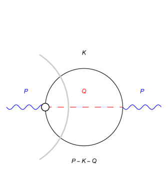
Figure 1: The contributions to the dark photon non time-ordered self energy due to scatterings of the form (3.2) involving two SM fermions (solid black lines) and a Higgs boson (dashed red line). Here, as well as in Figs. 2 and 3, all four-momenta flow from left to right. Here and in Figs. 2 we also show the corresponding cutting notation that holds at zero temperature.

In this case the DP is produced through scatterings of the form

$$ff\to H\mathcal{P},\qquad fH\to f\mathcal{P},$$ (3.2)

where the $f$s represent SM fermions. The corresponding contribution to the DP self-energy is given in Fig. 1 and its analytic expression is

$$[\Pi_{\mu\nu}^{<}(P)]_{fH}=-\frac{4C^{2}}{M^{4}}\int\frac{d^{4}K}{(2\pi)^{4}}\frac{d^{4}Q}{(2\pi)^{4}}\Delta_{B}^{<}(Q)\Delta_{F}^{<}(K)\Delta_{F}^{<}(P-K-Q)T_{\mu\nu}(P,K,Q),$$ (3.3)

where $C^{2}$ is a non-negative parameter defined in terms of the flavour matrices $C_{u}$, $C_{d}$ and $C_{e}$ by

$$C^{2}\equiv 2\left(3\,{\rm Tr}(C^{\dagger}_{u}C_{u}+C^{\dagger}_{d}C_{d})+\,{\rm Tr}(C^{\dagger}_{e}C_{e})\right),$$ (3.4)

$$\Delta_{B}^{<}(Q)\equiv(\theta(-Q_{0})+n_{B}(Q_{0}))2\pi\delta(Q^{2}-m^{2}),\quad\Delta^{<}_{F}(K)\equiv(\theta(-K_{0})-n_{F}(K_{0}))2\pi\delta(K^{2}-m^{2})$$

($m$ is a generic mass, which we neglect here, $m\to 0$) and

$$T_{\mu\nu}(P,K,Q)\equiv P^{\rho}P^{\lambda}\left(\,{\rm Tr}\left(\sigma_{\rho\mu}P_{R}\not{K}\sigma_{\lambda\nu}(\not{K}+\not{Q}-\not{P})\right)+\,{\rm Tr}\left(\sigma_{\rho\mu}P_{L}\not{K}\sigma_{\lambda\nu}(\not{K}+\not{Q}-\not{P})\right)\right).$$ (3.5)

Also, $\theta(x)$ is the Heaviside step function and $n_{B}(x)\equiv f_{B}(|x|)$, $n_{F}(x)\equiv f_{F}(|x|)$, where

$$f_{B}(x)\equiv\frac{1}{e^{\beta x}-1},\quad f_{F}(x)\equiv\frac{1}{e^{\beta x}+1},$$ (3.6)

are the Bose-Einstein and Fermi-Dirac distributions, respectively ($\beta\equiv 1/T$, where $T$ is the temperature, as usual). In (3.5) $P_{R}$ and $P_{L}$ are the right and left-handed projectors. We can simply ignore $P_{L}$ and $P_{R}$ and consider only the first (or equivalently the second) trace in Eq. (3.5) because the trace of six gamma matrices times $\gamma_{5}$ would produce a totally-antisymmetric Levi-Civita tensor and there are not enough independent four-momenta to have a non-vanishing contraction in $\eta^{\mu\nu}\Pi^{<}_{\mu\nu}(P)$. By using $\sigma_{\mu\nu}=i[\gamma_{\mu},\gamma_{\nu}]/2$ and performing the trace, we obtain

$$-\eta^{\mu\nu}T_{\mu\nu}(P,K,Q)=16K\cdot P(K\cdot P+Q\cdot P).$$ (3.7)

The integral in (3.3) receives contributions from three distinct integration regions, which correspond to three different scattering processes:

1. $K_{0}<0,\quad P_{0}-K_{0}-Q_{0}>0,\quad Q_{0}>0$;

2. $K_{0}>0,\quad P_{0}-K_{0}-Q_{0}<0,\quad Q_{0}>0$;

3. $K_{0}>0,\quad P_{0}-K_{0}-Q_{0}>0,\quad Q_{0}<0$.

These regions give the following contributions to the integrated DP production rate $\gamma_{d}$ per unit of volume (respectively for $i=1,2,3$):

$$[\gamma_{d}]_{fHi} = \frac{16C^{2}}{(2\pi)^{6}M^{4}}\int dp\,dk\,dq\,dz_{k}\,dz_{q}\frac{f_{i}(p,k,q,z_{k},z_{q})}{D_{i}(p,k,q,z_{k},z_{q})^{1/2}},$$ (3.8)

where

$$f_{1}(p,k,q,z_{k},z_{q}) = p^{2}k(1+z_{k})[pk(1+z_{k})-pq(1-z_{q})](1-f_{F}(k))f_{F}(p+k-q)f_{B}(q),$$

$$f_{2}(p,k,q,z_{k},z_{q}) = p^{2}k(1-z_{k})[pk(1-z_{k})+pq(1-z_{q})]f_{F}(k)(1-f_{F}(k+q-p))f_{B}(q),$$

$$f_{3}(p,k,q,z_{k},z_{q}) = p^{2}k(1-z_{k})[pq(1+z_{q})-pk(1-z_{k})]f_{F}(k)f_{F}(p-k+q)(1+f_{B}(q)),$$

$$D_{1}(p,k,q,z_{k},z_{q}) \equiv (1-z_{k}^{2})(1-z_{q}^{2})-\left[-1-z_{k}z_{q}+\frac{p}{q}(1+z_{k})-\frac{p}{k}(1-z_{q})\right]^{2},$$ (3.9)

$$D_{2}(p,k,q,z_{k},z_{q}) \equiv (1-z_{k}^{2})(1-z_{q}^{2})-\left[1-z_{k}z_{q}-\frac{p}{q}(1-z_{k})-\frac{p}{k}(1-z_{q})\right]^{2},$$ (3.10)

$$D_{3}(p,k,q,z_{k},z_{q}) \equiv (1-z_{k}^{2})(1-z_{q}^{2})-\left[-1-z_{k}z_{q}-\frac{p}{q}(1-z_{k})+\frac{p}{k}(1+z_{q})\right]^{2},$$ (3.11)

$z_{k}$ and $z_{q}$ are the cosines of the angles between $\vec{k}$ and $\vec{p}$ and $\vec{q}$ and $\vec{p}$, respectively and the integrals are performed on the intersection between the domains

$$0\leq p<\infty,\quad 0\leq k<\infty,\quad-1\leq z_{k}\leq 1,\quad 0\leq q<\infty,\quad-1\leq z_{q}\leq 1$$ (3.12)

and

$$D_{i}(p,k,q,z_{k},z_{q})\geq 0.$$ (3.13)

Computing numerically the integrals we obtain

$$[\gamma_{d}]_{fH}=\sum_{i=1}^{3}[\gamma_{d}]_{fHi}\simeq 85.3\frac{C^{2}T^{8}}{\pi^{6}M^{4}}.$$ (3.14)

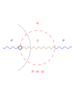
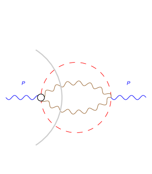
Figure 2: Left: The contributions to the dark photon non time-ordered self energy due to scatterings involving one $B$ (or one $W$) and two Higgs bosons. Right: The same as in the right plot, but with two (rather than one) $W$s.

3.1.2 $B$-Higgs scatterings

Let us now consider the DP production due to scattering involving one $B$ and two Higgs bosons (due to the operators with coefficients $c_{b}$ and $\tilde{c}_{b}$ in (2.1)):

$$BH\to H\mathcal{P},\qquad HH\to B\mathcal{P}.$$ (3.15)

The corresponding contribution to the DP self-energy is given in the left plot of Fig. 2 and its analytic expression $[\Pi_{\mu\nu}^{<}(P)]_{BH}$ produces the following contribution to the numerator in the right-hand side of (3.1)

$$-\eta^{\mu\nu}[\Pi_{\mu\nu}^{<}(P)]_{BH}=\frac{16(c_{b}^{2}+\tilde{c}_{b}^{2})}{M^{4}}\int\frac{d^{4}K}{(2\pi)^{4}}\frac{d^{4}Q}{(2\pi)^{4}}\Delta_{B}^{<}(Q)\Delta_{B}^{<}(K)\Delta_{B}^{<}(P-K-Q)(P\cdot Q)^{2}.$$ (3.16)

The interference term proportional to $c_{b}\tilde{c}_{b}$ vanishes because there are only three independent four-momenta, $P$, $Q$ and $K$, which are not enough to have a non-vanishing full contraction with only one Levi-Civita tensor. The contribution of $\tilde{c}_{b}^{2}$ is equal to that of $c_{b}^{2}$ because, with the definition of the dual field strength we are using, it turns out $B_{\mu\nu}B^{\mu\nu}=-\tilde{B}_{\mu\nu}\tilde{B}^{\mu\nu}$ and, in going from the field strength to its dual, one is only exchanging the electric and magnetic parts of the gauge field (modulo signs).

The integral in (3.16) receives contributions from the three distinct integration regions discussed in Sec. 3.1.1, which give the following contributions to $\gamma_{d}$ (respectively for $i=1,2,3$):

$$[\gamma_{d}]_{BHi} = \frac{4(c_{b}^{2}+\tilde{c}_{b}^{2})}{(2\pi)^{6}M^{4}}\int dp\,dk\,dq\,dz_{k}\,dz_{q}\frac{b_{i}(p,k,q,z_{k},z_{q})}{D_{i}(p,k,q,z_{k},z_{q})^{1/2}},$$ (3.17)

where

$$b_{1}(p,k,q,z_{k},z_{q}) = p^{3}q^{2}(1-z_{q})^{2}(1+f_{B}(k))f_{B}(p+k-q)f_{B}(q),$$

$$b_{2}(p,k,q,z_{k},z_{q}) = p^{3}q^{2}(1-z_{q})^{2}f_{B}(k)(1+f_{B}(k+q-p))f_{B}(q),$$

$$b_{3}(p,k,q,z_{k},z_{q}) = p^{3}q^{2}(1+z_{q})^{2}f_{B}(k)f_{B}(p-k+q)(1+f_{B}(q)),$$

again the functions $D_{i}$ are given in (3.9)-(3.11) and the integrals are performed on the intersection of the domains in (3.12) and (3.13). The numerical computation this time gives

$$[\gamma_{d}]_{BH}=\sum_{i=1}^{3}[\gamma_{d}]_{BHi}\simeq 40.5\frac{(c_{b}^{2}+\tilde{c}_{b}^{2})T^{8}}{\pi^{6}M^{4}}.$$ (3.18)

3.1.3 $W$-Higgs scatterings

The DP can also be produced in scatterings involving Higgs and $W$ bosons. In this case there are two contributions to the non time-ordered DP self energy.

One is analogous to that corresponding to scatterings involving the Higgs and the $B$ bosons, which have been discussed in Sec. 3.1.2. This contribution to $\gamma_{d}$ can be obtained by substituting $(c_{b},\tilde{c}_{b})\to(c_{w},\tilde{c}_{w})$ in (3.18):

$$[\gamma_{d}]_{WH}\simeq 40.5\frac{(c_{w}^{2}+\tilde{c}_{w}^{2})T^{8}}{\pi^{6}M^{4}}.$$ (3.19)

The other contribution is due to the non-Abelian nature of $W$, which leads to a term proportional to $[W_{\mu},W_{\nu}]$ in $W_{\mu\nu}$ and diagrams of the form given in Fig. 2 (on the right). This leads to a vanishing contribution to the differential production rate $\frac{d\gamma_{d}}{d^{3}p}$. Indeed, the tensorial structure of the corresponding contribution to the non time-ordered DP self energy, $[\Pi^{<}_{\mu\nu}(P)]_{WW}$, is proportional to $P_{\mu}P_{\nu}$ (as in both vertices there is a derivative acting on the massless DP field and no derivatives on the other fields) and so, since the DP is massless, $\eta^{\mu\nu}[\Pi^{<}_{\mu\nu}(P)]_{WW}=0$.

3.2 Dark-photon pair production

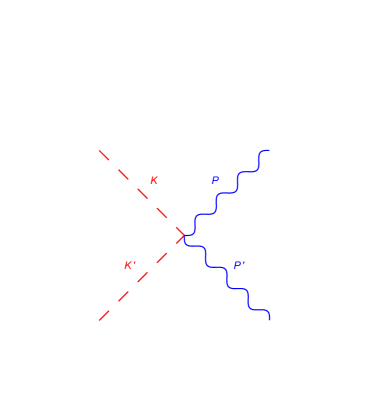
Figure 3: Dark-photon pair production due to Higgs pair annihilation.

Let us now turn to the contribution of the operators with coefficients $c_{p}$ and $\tilde{c}_{p}$ in (2.1). These lead to DP pair production through scatterings of the form (Higgs pair annihilation)

$$HH\to\mathcal{P}\mathcal{P},$$ (3.20)

whose Feynman diagram is given in Fig. 3.

The Feynman amplitude corresponding to Fig. 3 is

$$\mathcal{M}(HH\to\mathcal{P}\mathcal{P})=\frac{4i}{M^{2}}\left[c_{p}(P\cdot\varepsilon^{\prime}\,P^{\prime}\cdot\varepsilon-P\cdot P^{\prime}\,\varepsilon\cdot\varepsilon^{\prime})+\tilde{c}_{p}P_{\mu}P^{\prime}_{\sigma}\varepsilon_{\nu}\varepsilon^{\prime}_{\rho}\epsilon^{\mu\nu\rho\sigma}\right],$$ (3.21)

where $\varepsilon$ and $\varepsilon^{\prime}$ are the polarization vectors of the DPs with four-momenta $P$ and $P^{\prime}$, respectively. Summing over the respective polarizations $r$ and $r^{\prime}$ and multiplying by a factor of 2 to take into account that the Higgs is a doublet, one finds

$$2\sum_{rr^{\prime}}|\mathcal{M}(HH\to\mathcal{P}\mathcal{P})|^{2}=\frac{64(c_{p}^{2}+\tilde{c}_{p}^{2})(P\cdot P^{\prime})^{2}}{M^{4}}.$$ (3.22)

Again, the interference term (in this case proportional to $c_{p}\tilde{c}_{p}$) vanishes: after summing over the polarizations, all Lorentz indices of the four-momenta and of only one Levi-Civita tensor are contracted together and there are not enough independent four-momenta to have a non-vanishing result; also, the contribution of $\tilde{c}_{p}^{2}$ is equal to that of $c_{p}^{2}$ because $\mathcal{P}_{\mu\nu}\mathcal{P}^{\mu\nu}=-\mathcal{\tilde{P}}_{\mu\nu}\mathcal{\tilde{P}}^{\mu\nu}$.

The corresponding DP-pair production rate per unit of volume and averaged over the initial state with the Bose-Einstein distributions of the two Higgs particles is then

$$\gamma_{2d}=\int\frac{d^{3}k}{2(2\pi)^{3}E}f_{B}(E)\frac{d^{3}k^{\prime}}{2(2\pi)^{3}E^{\prime}}f_{B}(E^{\prime})\,I(Q^{2}),$$ (3.23)

where $E$ and $E^{\prime}$ are the energies of the Higgs bosons with four-momenta $K$ and $K^{\prime}$ respectively and $I$ is a Lorentz-invariant function of $Q\equiv K+K^{\prime}$ given by

$$I(Q^{2})=\int\frac{d^{3}p}{2(2\pi)^{3}E_{p}}\frac{d^{3}p^{\prime}}{2(2\pi)^{3}E^{\prime}_{p}}(2\pi)^{4}\delta(P+P^{\prime}-Q)\,2\sum_{rr^{\prime}}|\mathcal{M}(HH\to\mathcal{P}\mathcal{P})|^{2}$$ (3.24)

($E_{p}$ and $E_{p}^{\prime}$ are the energies of the two DPs). By performing the integrals over $\vec{p}$ and $\vec{p}\,^{\prime}$ one obtains

$$I(Q^{2})=\frac{c_{p}^{2}+\tilde{c}_{p}^{2}}{\pi}\left(\frac{Q^{2}}{M^{2}}\right)^{2}$$ (3.25)

and, integrating over $\vec{k}$ and $\vec{k}\,^{\prime}$,

$$\gamma_{2d}=\frac{(c_{p}^{2}+\tilde{c}_{p}^{2})\pi^{3}T^{8}}{675M^{4}}.$$ (3.26)

Summary

The full rate of DP thermal production per unit of volume is obtained by summing the contributions obtained in the previous sections 3.1 and 3.2:

$$\gamma_{d}=\frac{\alpha T^{8}}{\pi^{3}M^{4}},$$ (3.27)

where

$$\alpha\simeq\left[2.75\,C^{2}+1.31(c_{b}^{2}+\tilde{c}_{b}^{2}+c_{w}^{2}+\tilde{c}_{w}^{2})+\frac{2\pi^{6}(c_{p}^{2}+\tilde{c}_{p}^{2})}{675}\right]$$ (3.28)

and $C^{2}$ is defined in Eq. (3.4).

4 Dark-photon yield

Let us now compute the DP yield as a function of the temperature, which is important for determining the DP abundance during the cosmological history.

After inflation and reheating have taken place, the relevant Boltzmann equation is

$$sHT\frac{dY_{d}}{dT}=-\gamma_{d}\left(1-\frac{Y_{d}}{Y_{d}^{\rm eq}}\right).$$ (4.1)

The various quantities that appear in this equation are defined as follows.

• $s$ is the entropy density of the relativistic SM plasma $s=2\pi^{2}g_{\rm SM}T^{3}/45$, with $g_{\rm SM}\simeq 427/4$.

• $H$ is the Hubble rate $H=\sqrt{\rho/3}/M_{P}$, where $M_{P}$ is the reduced Planck mass and $\rho\simeq\pi^{2}g_{\rm SM}T^{4}/30$.

• The DP yield $Y_{d}$ is defined as the comoving number density, $Y_{d}\equiv n_{d}/s$, where $n_{d}$ is the DP number density with equilibrium value $n_{d}^{\rm eq}=2\zeta(3)T^{3}/\pi^{2}$ and $\zeta(s)$ is the Riemann zeta function. So $Y_{d}^{\rm eq}=n_{d}^{\rm eq}/s\simeq 0.005$.

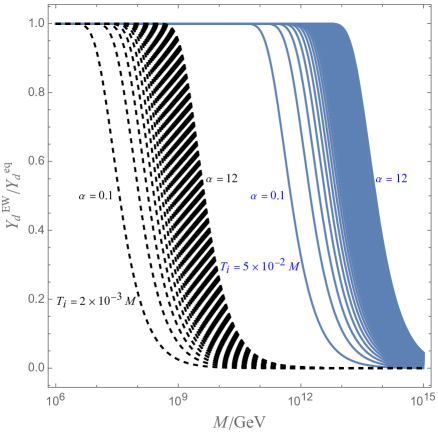
Figure 4: The dark-photon yield at the EW scale $T\sim 250$ GeV as a function of $M$ setting $Y_{d}(T_{i})=0$ at the initial temperature $T_{i}$. The parameter $\alpha$ is defined in Eq. (3.28) and is increased in the plot with steps of length $0.2$.

Using (3.27), the general solution of Eq. (4.1) is

$$Y_{d}(T)=Y_{d}^{\rm eq}+(Y_{i}-Y_{d}^{\rm eq})\exp\left(\frac{45}{\pi^{6}}\sqrt{\frac{5}{2g_{\rm SM}^{3}}}\frac{\alpha}{Y_{d}^{\rm eq}}\frac{M_{P}}{M}\left(\frac{T^{3}-T_{i}^{3}}{M^{3}}\right)\right),$$ (4.2)

where $Y_{i}\equiv Y_{d}(T_{i})$ is the initial condition at a given initial temperature $T_{i}$. In Fig. 4 the value of $Y_{d}$ at the EW scale $T\sim 250$ GeV (above all SM particle masses), which is denoted $Y_{d}^{\rm EW}$, is plotted as a function of $M$ setting $Y_{i}=0$. By increasing $Y_{i}$ and/or $T_{i}$ the value of $Y_{d}(T)$ increases as clear from (4.2) because $Y_{i}$ is always taken to be smaller than $Y_{d}^{\rm eq}$. Note that, if $Y_{d}$ was ever zero when the effective Lagrangian (2.1) is valid, the corresponding value of the temperature should be the largest possible one in the range of temperatures where the effective field theory is valid because the solution in (4.2) is a decreasing function of $T$ (recall $Y_{i}<Y_{d}^{\rm eq}$ and obviously $Y_{d}(T)\geq 0$). So (4.2) and Fig. 4 show that DPs are copiously produced and $Y_{d}$ can reach its equilibrium value at temperatures above all SM particle masses even if $M$ is several orders of magnitude above the EW scale. Also, note that $Y_{d}(T)$ decreases exponentially as $T$ increases and so the DP production is most effective at large temperatures, which are as close as possible to the cutoff. This justifies our approximation in which all SM particle masses are neglected in the calculation of the thermal production rate of Sec. 3.

Any given DP model predicts specific coefficients in (2.1) and so a specific value of $\alpha$; one can then compute for any model the DP yield by using Fig. 4 or, more generally, Eq. (4.2).

5 Dark-photon contribution to $N_{\rm eff}^{(\nu)}$

After being produced, the massless DP contributes to the effective number of neutrinos $N_{\rm eff}^{(\nu)}$. Let us determine this contribution here.

We start by computing today’s DP temperature. In order to do so one needs to know how many SM degrees of freedom were relativistic at the time of DP decoupling. From the effective Lagrangian in (2.1) one sees that all DP interactions with the SM particles need at least one Higgs field. Therefore, the effective Lagrangian in (2.1) implies that the DP decoupled at a (photon) temperature that, at leading order, is not much smaller than the Higgs mass, $T\gtrsim M_{h}$. Indeed, by including the non-vanishing value of $M_{h}$ in the calculations of Sec. 3 one finds that the thermal production is exponentially suppressed by Boltzmann factors $\sim\exp(-M_{h}/T)$ for $T<M_{h}$. Going to next-to-leading order by switching on SM couplings and/or including effective operators of dimension greater than six, one can check using Eq. (4.1) that the DP always decoupled at a temperature not much smaller than the Higgs mass requiring $M$ to be sufficiently above the TeV scale. This requirement ensures that the observational exclusion limits [2] are satisfied (recall that the messenger fields have sizable couplings to the SM). At a temperature $T_{1}$ just above the DP decoupling temperature when all (or almost all) SM particles were relativistic the total entropy density of the relativistic plasma was

$$s_{1}\simeq(g_{\rm SM}+2)T_{1}^{3}\frac{2\pi^{2}}{45}.$$ (5.1)

After $e^{+}e^{-}$ annihilation the neutrinos decoupled with a temperature $T_{\nu}=(4/11)^{1/3}T$, where $T$, as always, is the photon temperature. At these later times the entropy density was

$$s_{2}=\left(2T^{3}+\frac{7}{8}\times 6T_{\nu}^{3}+2T_{d}^{3}\right)\frac{2\pi^{2}}{45}=\left(\frac{43}{11}T^{3}+2T_{d}^{3}\right)\frac{2\pi^{2}}{45},$$ (5.2)

where $T_{d}$ is the DP temperature. From the time when the entropy density was $s_{1}$ until today the DP was decoupled and, therefore, was not reheated by particle annihilations. As a result $T_{d}$ scaled at those times as $1/a$, where $a$ is the (cosmological) scale factor. So $T_{1}a_{1}=T_{d}a_{0}$, where $a_{1}$ and $a_{0}$ are the values of the scale factor corresponding to $T_{1}$ and to times after $e^{+}e^{-}$ annihilation, respectively. From entropy conservation, $s_{1}a_{1}^{3}=s_{2}a_{0}^{3}$, it follows

$$T_{d}=\left(\frac{43}{11g_{\rm SM}}\right)^{1/3}T.$$ (5.3)

This DP temperature corresponds today to a contribution to the effective number of neutrinos $N_{\rm eff}^{(\nu)}$ given by

$$\Delta N_{\rm eff}^{(\nu)}=\frac{8}{7}\left(\frac{T_{d}}{T_{\nu}}\right)^{4}=\frac{8}{7}\left(\frac{43}{4g_{\rm SM}}\right)^{4/3},$$ (5.4)

which, using $g_{\rm SM}=427/4$, gives

$$\Delta N_{\rm eff}^{(\nu)}\simeq 0.0535.$$ (5.5)

This contribution is twice that of the axion of Quantum Chromodynamics (QCD) determined in [37] because the DP has two degrees of freedom, but otherwise the DP has properties similar to those of the QCD axion for temperatures above the QCD phase transition. Adding the contribution in (5.4) to the SM value 3.044 recently computed in [39, 40, 41, 42], one obtains $N_{\rm eff}^{(\nu)}\simeq 3.1$ in good agreement with the most precise constraint $N_{\rm eff}^{(\nu)}=2.99\pm 0.17$ published by the Planck collaboration in 2018 [43].

Future measurements of $N_{\rm eff}^{(\nu)}$ will be able to test the DP scenario. For example, the CMB-S4 project (the “Stage-4” ground-based cosmic microwave background experiment) expects to reach a sensitivity around 0.02-0.03 for $N_{\rm eff}^{(\nu)}$ [44].

6 Conclusions

In this paper the thermal production rate of massless DPs has been computed at leading order taking into account the contribution of all SM particles and using a model-independent effective field theory point of view. Moreover, the corresponding DP yield and DP contribution to $N_{\rm eff}^{(\nu)}$ have been calculated too.

In order to perform these computations, in Sec. 2 the most general effective field theory describing all possible interactions with all SM fields up to dimension-six operators has been identified. No dimension-five operators can be constructed describing the interactions of the DP with SM fields only. In all dimension-six operators the Higgs field appears too.

In Sec. 3 the DP thermal production rate per unit of volume, $\gamma_{d}$, has been computed and the final result has been summarized in Eqs. (3.27) and (3.28). The rate grows with temperature as $T^{8}/M^{4}$ with a coefficient $\alpha/\pi^{3}$ that can naturally be as large as$\leavevmode\nobreak\ \sim 10$: this order of magnitude is obtained by assuming all coefficients ($c_{i}$, $\tilde{c}_{i}$, with $i=b,w,p$, and $C_{u}$, $C_{d}$ and $C_{e}$) of the dimension-six operators in (2.1) to be of order 1. Of course, some or many coefficients could be zero in some specific models and $\alpha$ can be smaller in those cases.

The corresponding DP yield $Y_{d}$ has been computed in Sec. 4 solving analytically the relevant Boltzmann equation. The analytic solution is given in (4.2) and the value of $Y_{d}$ at the EW scale is plotted as a function of $M$ in Fig. 4. These results show that the DP production is most effective at large temperatures, which are as close as possible to the cutoff compatibly with the validity of the effective field theory, and $Y_{d}$ can reach its equilibrium value at temperatures above all SM particle masses, even if $M$ is several orders of magnitude above the EW scale. As a result, we also note that the DP production computed here also applies to a massive DP as long as its mass is very small compared to the large temperatures at which the production is maximized. For example, this is always the case when the DP mass is much below the EW scale. For previous computations of massive DP thermal production for temperatures much below the EW scale see Refs. [23, 27, 35, 25].

Finally, the corresponding DP contribution to $N_{\rm eff}^{(\nu)}$ has been determined in Sec. 5 (see Eq. (5.4)). This prediction is in good agreement with current observations and will be tested with future measurements such as those of CMB-S4.

Acknowledgments

I thank Massimo Bianchi and Marina Migliaccio for useful discussions. This work has been partially supported by the grant DyConn from the University of Rome Tor Vergata.

References

- [1] B. Holdom, “Two U(1)’s and Epsilon Charge Shifts,” Phys. Lett. B 166 (1986), 196-198 doi:10.1016/0370-2693(86)91377-8
- [2] M. Fabbrichesi, E. Gabrielli and G. Lanfranchi, “The Dark Photon,” doi:10.1007/978-3-030-62519-1 [arXiv:2005.01515].
- [3] Z. Berezhiani, “Mirror world and its cosmological consequences,” Int. J. Mod. Phys. A 19 (2004), 3775-3806 doi:10.1142/S0217751X04020075 [arXiv:hep-ph/0312335].
- [4] Z. Berezhiani and A. Lepidi, “Cosmological bounds on the ’millicharges’ of mirror particles,” Phys. Lett. B 681 (2009), 276-281 doi:10.1016/j.physletb.2009.10.023 [arXiv:0810.1317].
- [5] A. Salvio and A. Strumia, “Agravity,” JHEP 06 (2014), 080 doi:10.1007/JHEP06(2014)080 [arXiv:1403.4226].
- [6] S. A. Abel and B. W. Schofield, “Brane anti-brane kinetic mixing, millicharged particles and SUSY breaking,” Nucl. Phys. B 685 (2004), 150-170 doi:10.1016/j.nuclphysb.2004.02.037 [arXiv:hep-th/0311051].
- [7] S. A. Abel, J. Jaeckel, V. V. Khoze and A. Ringwald, “Illuminating the Hidden Sector of String Theory by Shining Light through a Magnetic Field,” Phys. Lett. B 666 (2008), 66-70 doi:10.1016/j.physletb.2008.03.076 [arXiv:hep-ph/0608248].
- [8] S. A. Abel, M. D. Goodsell, J. Jaeckel, V. V. Khoze and A. Ringwald, “Kinetic Mixing of the Photon with Hidden U(1)s in String Phenomenology,” JHEP 07 (2008), 124 doi:10.1088/1126-6708/2008/07/124 [arXiv:0803.1449].
- [9] M. Goodsell, J. Jaeckel, J. Redondo and A. Ringwald, “Naturally Light Hidden Photons in LARGE Volume String Compactifications,” JHEP 11 (2009), 027 doi:10.1088/1126-6708/2009/11/027 [arXiv:0909.0515].
- [10] A. Salvio, “A fundamental QCD axion model,” Phys. Lett. B 808 (2020), 135686 doi:10.1016/j.physletb.2020.135686 [arXiv:2003.10446].
- [11] A. Ghoshal and A. Salvio, “Gravitational waves from fundamental axion dynamics,” JHEP 12 (2020), 049 doi:10.1007/JHEP12(2020)049 [arXiv:2007.00005].
- [12] S. Weinberg, “The Cosmological Constant Problem,” Rev. Mod. Phys. 61 (1989), 1-23 doi:10.1103/RevModPhys.61.1
- [13] S. Weinberg, “Anthropic Bound on the Cosmological Constant,” Phys. Rev. Lett. 59 (1987), 2607 doi:10.1103/PhysRevLett.59.2607
- [14] V. Agrawal, S. M. Barr, J. F. Donoghue and D. Seckel, “Viable range of the mass scale of the standard model,” Phys. Rev. D 57 (1998), 5480-5492 doi:10.1103/PhysRevD.57.5480 [arXiv:hep-ph/9707380].
- [15] G. D’Amico, A. Strumia, A. Urbano and W. Xue, “Direct anthropic bound on the weak scale from supernovæ explosions,” Phys. Rev. D 100 (2019) no.8, 083013 doi:10.1103/PhysRevD.100.083013 [arXiv:1906.00986].
- [16] A. Baldazzi, O. Melichev and R. Percacci, “Metric-Affine Gravity as an effective field theory,” Annals Phys. 438 (2022), 168757 doi:10.1016/j.aop.2022.168757 [arXiv:2112.10193].
- [17] D. E. Neville, “A Gravity Lagrangian With Ghost Free Curvature**2 Terms,” Phys. Rev. D 18 (1978), 3535 doi:10.1103/PhysRevD.18.3535.
- [18] R. Percacci and E. Sezgin, “New class of ghost- and tachyon-free metric affine gravities,” Phys. Rev. D 101 (2020) no.8, 084040 doi:10.1103/PhysRevD.101.084040 [arXiv:1912.01023].
- [19] D. E. Neville, “Gravity Theories With Propagating Torsion,” Phys. Rev. D 21 (1980), 867 doi:10.1103/PhysRevD.21.867
- [20] D. E. Neville, “Spin-2 propagating torsion,” Phys. Rev. D 23 (1981), 1244-1249 doi:10.1103/PhysRevD.23.1244
- [21] A. S. Belyaev, I. L. Shapiro and M. A. B. do Vale, “Torsion phenomenology at the LHC,” Phys. Rev. D 75 (2007), 034014 doi:10.1103/PhysRevD.75.034014 [arXiv:hep-ph/0701002].
- [22] G. Pradisi and A. Salvio, “(In)equivalence of metric-affine and metric effective field theories,” Eur. Phys. J. C 82 (2022) no.9, 840 doi:10.1140/epjc/s10052-022-10825-9 [arXiv:2206.15041].
- [23] J. Redondo and M. Postma, “Massive hidden photons as lukewarm dark matter,” JCAP 02 (2009), 005 doi:10.1088/1475-7516/2009/02/005 [arXiv:0811.0326].
- [24] H. An, M. Pospelov, J. Pradler and A. Ritz, “Direct Detection Constraints on Dark Photon Dark Matter,” Phys. Lett. B 747 (2015), 331-338 doi:10.1016/j.physletb.2015.06.018 [arXiv:1412.8378].
- [25] A. Fradette, M. Pospelov, J. Pradler and A. Ritz, “Cosmological Constraints on Very Dark Photons,” Phys. Rev. D 90 (2014) no.3, 035022 doi:10.1103/PhysRevD.90.035022 [arXiv:1407.0993].
- [26] B. A. Dobrescu, “Massless gauge bosons other than the photon,” Phys. Rev. Lett. 94 (2005), 151802 doi:10.1103/PhysRevLett.94.151802 [arXiv:hep-ph/0411004].
- [27] H. Vogel and J. Redondo, “Dark Radiation constraints on minicharged particles in models with a hidden photon,” JCAP 02 (2014), 029 doi:10.1088/1475-7516/2014/02/029 [arXiv:1311.2600 [hep-ph]].
- [28] R. Foot and S. Vagnozzi, “Dissipative hidden sector dark matter,” Phys. Rev. D 91 (2015), 023512 doi:10.1103/PhysRevD.91.023512 [arXiv:1409.7174].
- [29] P. Adshead, P. Ralegankar and J. Shelton, “Dark radiation constraints on portal interactions with hidden sectors,” JCAP 09 (2022), 056 doi:10.1088/1475-7516/2022/09/056 [arXiv:2206.13530].
- [30] M. L. Bellac, “Thermal Field Theory,” Cambridge University Press, 2011, ISBN 978-0-511-88506-8, 978-0-521-65477-7 doi:10.1017/CBO9780511721700
- [31] R. L. Kobes and G. W. Semenoff, “Discontinuities of Green Functions in Field Theory at Finite Temperature and Density,” Nucl. Phys. B 260 (1985), 714-746 doi:10.1016/0550-3213(85)90056-2
- [32] R. L. Kobes and G. W. Semenoff, “Discontinuities of Green Functions in Field Theory at Finite Temperature and Density. 2,” Nucl. Phys. B 272 (1986), 329-364 doi:10.1016/0550-3213(86)90006-4
- [33] A. Salvio, P. Lodone and A. Strumia, “Towards leptogenesis at NLO: the right-handed neutrino interaction rate,” JHEP 08 (2011), 116 doi:10.1007/JHEP08(2011)116 [arXiv:1106.2814].
- [34] J. Jaeckel, J. Redondo and A. Ringwald, “Signatures of a hidden cosmic microwave background,” Phys. Rev. Lett. 101 (2008), 131801 doi:10.1103/PhysRevLett.101.131801 [arXiv:0804.4157].
- [35] K. W. Ng, H. Tu and T. C. Yuan, “Dark photons as fractional cosmic neutrino masquerader,” JCAP 09 (2014), 035 doi:10.1088/1475-7516/2014/09/035 [arXiv:1406.1993].
- [36] M. Ibe, S. Kobayashi, Y. Nakayama and S. Shirai, “Cosmological constraint on dark photon from Neff,” JHEP 04 (2020), 009 doi:10.1007/JHEP04(2020)009 [arXiv:1912.12152].
- [37] A. Salvio, A. Strumia and W. Xue, “Thermal axion production,” JCAP 01 (2014), 011 doi:10.1088/1475-7516/2014/01/011 [arXiv:1310.6982].
- [38] F. D’Eramo, F. Hajkarim and S. Yun, “Thermal Axion Production at Low Temperatures: A Smooth Treatment of the QCD Phase Transition,” Phys. Rev. Lett. 128 (2022) no.15, 152001 doi:10.1103/PhysRevLett.128.152001 [arXiv:2108.04259].
- [39] J. J. Bennett, G. Buldgen, M. Drewes and Y. Y. Y. Wong, “Towards a precision calculation of the effective number of neutrinos in the Standard Model I: the QED equation of state,” JCAP 03 (2020), 003 doi:10.1088/1475-7516/2020/03/003 [arXiv:1911.04504].
- [40] K. Akita and M. Yamaguchi, “A precision calculation of relic neutrino decoupling,” JCAP 08 (2020), 012 doi:10.1088/1475-7516/2020/08/012 [arXiv:2005.07047].
- [41] J. Froustey, C. Pitrou and M. C. Volpe, “Neutrino decoupling including flavour oscillations and primordial nucleosynthesis,” JCAP 12 (2020), 015 doi:10.1088/1475-7516/2020/12/015 [arXiv:2008.01074].
- [42] J. J. Bennett, G. Buldgen, P. F. De Salas, M. Drewes, S. Gariazzo, S. Pastor and Y. Y. Y. Wong, “Towards a precision calculation of in the Standard Model II: Neutrino decoupling in the presence of flavour oscillations and finite-temperature QED,” JCAP 04 (2021), 073 doi:10.1088/1475-7516/2021/04/073 [arXiv:2012.02726].
- [43] N. Aghanim et al. [Planck], “Planck 2018 results. VI. Cosmological parameters,” Astron. Astrophys. 641 (2020), A6 [erratum: Astron. Astrophys. 652 (2021), C4] doi:10.1051/0004-6361/201833910 [arXiv:1807.06209].
- [44] K. N. Abazajian et al. [CMB-S4], “CMB-S4 Science Book, First Edition,” [arXiv:1610.02743].
- [45]