Anisotropic fluctuations of angular momentum of heavy quarks in the Glasma
Abstract
We study the evolution of the angular momentum of the heavy quarks in the very early stage of high energy nuclear collisions, in which the background is made of evolving Glasma fields. Given the novelty of the problem, we limit ourselves to the use of toy heavy quarks with a large, unphysical mass, in order to implement the kinetic equations for the angular momentum in the non-relativistic limit. We find that as a consequence of the anisotropy of the background fields, angular momentum fluctuations are also anisotropic: we understand this in simple terms relating the fluctuations of the angular momentum, , to those of linear momentum. While orbital angular momentum diffuses and develops substantial fluctuations and anisotropies, the spin does not. Hence, we can identify the fluctuations of with those of the total angular momentum . Therefore, our study suggests that the total angular momentum of the heavy quarks in the early stage of high energy nuclear collisions will present anisotropic fluctuations.
pacs:
12.38.Aw, 12.38.MhI Introduction
To study the fundamentals of nature, to be precise in the context of our work, Quantum Chromodynamic (QCD) matter, high-energy nuclear collisions have worked as great tools. The ultrarelativistic heavy-ion collisions performed at Relativistic Heavy Ion Collider (RHIC) and Large Hadron Collider (LHC) made it possible to recreate conditions similar to those of the early universe. The term little-bang that is often used to describe the shattering of two relativistic nuclei confirms the formation of a deconfined state of quarks and gluons known as Quark-Gluon Plasma (QGP) [1, 2]. The creation of locally equilibrated QGP in these collision experiments is a consequence of very complicated dynamics that happens to occur within a time scale of 1 fm/c. The very earliest phase is the span of highly non-equilibrium gluon fields and we call it the initial condition for the thermalized QGP. This initial condition, famously known in the literature as Glasma, is recognized as the pre-equilibrium stage just after the collision of nuclei where the density of chromodynamic fields is extremely high. The research of this initial condition and its decay to a nearly perfect fluid QGP is of immense interest to physicists worldwide to explore the QCD phase diagram in more detail.
The scenario before the collision is described using effective theory of Color-Glass Condensate (CGC) [3, 4, 5, 6, 7, 8, 9] which leads to the formation of Glasma [10, 11, 12, 13, 14, 15, 16, 17, 18, 19, 20]. CGC is the description of high-energy partons in the saturation regime. The two colliding nuclei are modeled as two sheets of colored glass where the fast parton dynamics seem to stop and they act as static sources for low momentum gluons. As a result of collision of two CGC sheets, we get a configuration of strong classical gluon fields, namely Glasma. The Glasma consists of longitudinal color-electric and color-magnetic fields in the weak coupling regime and is characterized by a large gluon occupation number. The evolution of these fields is studied using classical Yang-Mills (CYM) equations. We are interested in the physics of the non-equilibrium phase when the dynamics is of dense chromodynamic fields rather than partons. In this article, we use the notation EvGlasma for the evolving Glasma fields and reserve the name Glasma for the initial condition.
Heavy quarks [21, 22, 23, 24, 25, 26, 27, 28, 29, 30, 31, 32, 33, 34, 35, 36, 37, 38, 39, 40, 41, 42, 43, 44, 45, 46, 47, 48] produced in the very early phase of the ultra-relativistic heavy-ion collisions are efficient probes each for the pre-equilibrium Glasma phase and the equilibrated quark-gluon plasma (QGP). The charm and the beauty quarks are the most interesting quarks due to their very small formation time computed by , where is the mass of the heavy quark. It gives fm/c for charm quarks and fm/c for beauty quarks. Hence, due to their large masses, they are formed immediately just after the collision, so, they can propagate in the evolving gluonic medium to probe their evolution. Along with that, heavy quarks carry negligible color current and rarely interact among themselves due to their small number and large mass. So, they provide no disturbance to the evolving gluon fields and behave as ideal probes of these fields in the early stages of high energy collisions.
The prime aim of this article is to study the behaviour of the angular momentum of the heavy quarks (HQs) in presence of the coherent gluon fields that form in the early stage of the high energy nuclear collisions, and that approximately live up to fm/c in the case of collisions at the RHIC energy and up to fm/c for collisions at the LHC energy. For simplicity, we limit ourselves to the case of non-relativistic heavy quarks, leaving the full relativistic case to a future study. It is already known that the coherent gluon fields of the evolving Glasma affect the diffusion of momentum of HQs [49, 50, 51, 52, 53, 54, 55, 56]; it is therefore of a certain interest to extend the subject of the previous studies and analyze the behavior of other quantities: among them, we believe that angular momentum spreading of HQs is potentially interesting. Since ours is a first study about the subject, we limit ourselves to simulate the system in a static box; moreover, the system we simulate has both in the gluon and in the HQs sectors: the inclusion of a finite is feasible but far from being trivial and will be the subject of future studies. Our main purpose here is to show how the anisotropic momentum diffusion of HQs in the evolving Glasma fields leads to anisotropic fluctuations of the angular momentum of HQs.
The plan of the article is as follows: in section II, we briefly present the initial condition, namely the Glasma fields, as well as their evolution, and write the kinetic equations for the HQs. In section III, we present our results for the diffusion of the total angular momentum of HQs in the evolving Glasma. Finally, we summarize our results presenting the anisotropy of the fluctuations of the components of . In section IV, we conclude our work and discuss the possible future improvements.
II Formalism
II.1 Notations and conventions
We work in natural units, explicitly, . The Greek indices such as , can take the values 0, 1, 2, 3; where 0 represents the temporal coordinate and 1, 2, 3 represent the spatial coordinates. On the other hand, the Latin alphabets, namely , , numerate the Cartesian spatial coordinates and can take values 1, 2, 3 only. Keeping Einstein’s summation convention in mind, we assume repeated indices are summed up. denotes the three dimensional Levi-Civita tensor with .
The indices , , having values are reserved for the color components of the group in the adjoint representation. ’s are the generators of the group following the normalisation condition and the commutation relation where are the completely anti-symmetric structure constants.
The QCD covariant derivative is
| (1) |
This allows us to define the kinematic 4-momentum
| (2) |
where denotes the canonical momentum. This gives in particular
| (3) |
where
| (4) |
Using 3-dimensional notation, we can rewrite Eq. (3) as
| (5) |
II.2 Glasma and its evolution
The initialization of the gluon fields we adopt in our study is based on the McLerran-Venugopalan (MV) model [3, 4, 5] in which the collision of high energy nuclei is described within the framework of the color-glass condensate (CGC). CGC is an effective field theory based on the separation of scales of nucleon momentum fraction. The two colliding objects are viewed as two thin Lorentz-contracted sheets of a colored glass. CGC enables us to treat the two degrees of freedom, i.e., very fast color sources and slow color fields on different footing. The fast partons, as a result of time dilation appear to be frozen and act as the sources of the slow dynamical gluon fields in the saturation regime. These dominating gluon fields behave classically due to their high occupation numbers.
As per the MV model, the color charge densities of fast partons vary randomly on nuclei. Hence, it is assumed that the static color charge densities on colliding entity are normally distributed random variables. The first and second moments of the color charge density are given by
| (6) | |||||
| (7) |
where is the Yang-Mills coupling constant and denotes the color charge density of object in the transverse plane, which is of the order of the saturation momentum ; and correspond to the adjoint color index. For the sake of simplicity, we limit ourselves to the color group, hence, we get .
Within the MV model, the non-abelian interaction of the color fields present in the nuclei before the collision at produces a new set of strong, longitudinal fields after the collision at , that serves as the initial condition for the problem at hand: this new set of fields is called the Glasma. In order to determine the Glasma, we start by solving the two-dimensional Poisson’s equation for the gauge potential generated by the static color charge distribution of the nuclei,
| (8) |
where are the two colliding objects. The corresponding Wilson lines are computed by
| (9) | |||||
| (10) |
The Wilson lines are used to calculate the transverse components of the gauge fields present on the colliding object. The pre-collision gauge fields are given by
| (11) | |||||
| (12) |
where . We assume the z-direction to be the direction of receding of two nuclei. In terms of these gauge fields, the solution of the classical Yang-Mills (CYM) equations in the forward light cone at initial time, namely the Glasma gauge potentials, are given by
| (13) | |||||
| (14) |
Hence, the initial longitudinal Glasma fields are calculated by
| (15) | |||||
| (16) |
the transverse fields are absent in the initial condition.
After settling down the initial conditions for the Glasma, we study its evolution by virtue of the classical Yang-Mills (CYM) equations. We work in the temporal gauge , which leaves us with the freedom to perform time-independent gauge rotations. In this gauge, the Hamiltonian density is given by [57]
| (17) |
The field strength tensor is given by
| (18) |
where for gauge theory. Hence, the equations of motion for the dynamical evolution of Glasma, namely the CYM equations become
| (19) | |||
| (20) |
II.3 Evolution of heavy quarks in the classical, non-relativistic limit
We now quickly discuss the derivation of the non-relativistic equations of motion of the HQs in the evolving Glasma fields. This derivation is pretty standard and was presented years ago in the relativistic case [58], therefore here we limit ourselves to show only a few key steps of the derivation.
The non-relativistic Dirac equation for a free HQ reads
| (21) |
where denotes the upper component of the Dirac spinor and
| (22) |
and is the heavy quark mass and is the non-relativistic energy eigenvalue.
As in the case of the interaction with an external electromagnetic field, we can account for the interaction with a gluon field by the replacement in (22), in agreement with gauge invariance, see Eq. (5). This gives, in the gauge ,
| (23) |
We can extract the interaction of spin with the color-magnetic field from the operator on the right hand side of Eq. (23) as follows. Firstly, we note that , and using , we can write
| (24) | |||||
The first addendum on the right hand side of the above equation describes the diamagnetic interaction with the external field and does not need further manipulations. The second addendum represents the paramagnetic interaction.
Following the same, well-known steps used to derive the non-relativistic limit of the Dirac equation in an external electromagnetic field, we get
| (25) |
where the magnetic part of field strength tensor is defined as
| (26) |
Putting
| (27) |
we get eventually
| (28) |
with . We notice that the operator is not diagonal in color space, due to the matrices in . This implies that in general the eigenstates of and are not eigenstates of , therefore time evolution will mix the different colors.
The classical equations of motion of momentum, angular momentum and color charge can be obtained easily starting with the Hamiltonian in Eq. (28), by deriving the relevant Heisenberg equations then writing them in the classical limit. This is an easy exercise that was done already in the relativistic case [58], hence we can limit ourselves to quote the final results, namely
| (29) | |||||
| (30) | |||||
| (31) | |||||
| (32) | |||||
| (33) |
Here , with , denotes the classical quark color charge, where stand for the generators normalized as . Equations (31) and (32) imply and ; therefore, they describe the motion of the color charge and of the spin of the heavy quarks on the hypersphere and on the sphere respectively. Moreover, the right hand side of Eq. (33) corresponds to the torque of the force acting on the HQs. This set of equation will be used to study the evolution of the HQs in the background of the evolving Glasma fields. In the relativistic regime the equations are more complicated; in particular, Eq. (32) becomes a BMT-like equation [59] with terms, of order , that couple spin to momentum [58]: this particular term does not appear in the non-relativistic limit as it is subleading in the limit. Hence, our equations give the complete dynamics of the HQs in the non-relativistic limit.
II.4 Anisotropic fluctuations of
The main scope of this study is to highlight the anisotropic fluctuations of angular momentum that could form in the very early stage of high energy nuclear collisions. The system we study is characterized by a vanishing average angular momentum, namely , both for the HQs and the background gluon fields; however, fluctuations of of the HQs are produced as a result of the interaction with the gluon fields. These fluctuations are anisotropic and in fact they can be related in a simple, semi-quantitative way to the anisotropy of the momentum broadening of HQs and to the geometry of the collision.
As a matter of fact, which gives
| (34) |
where the last equality stands in the assumption that the components of are uncorrelated (this hypothesis is confirmed by a direct calculation in our simulations); and correspond to the coordinates of the quark, which are uncorrelated with momenta (this assumption breaks down if ). Similarly we can write
| (35) |
Assuming that HQs are distributed uniformly in the box, and denoting by and the transverse and longitudinal half-sides of the box respectively, we can integrate Eqs. (34) and (35) over the entire box and divide by the volume of the box, ; then we get
| (36) | |||||
| (37) |
Taking into account that (the transverse momentum distribution is isotropic, as confirmed by the numerical simulations) and that , we get
| (38) | |||||
| (39) |
We thus define the anisotropy parameter
| (40) |
by virtue of Eqs. (38) and (39) we can write
| (41) |
The result (41) shows that can be nonzero either as a result of the interaction of the HQs with the anisotropic gluon fields, which gives as shown in Fig. 1, or because of the geometry of the fireball created in the collision that in general, and in particular in the pre-equilibrium stage, satisfies ; in the case of the evolving Glasma fields both conditions contribute to . In the limit , which is appropriate for the early stage of heavy nuclei, we get
| (42) |
In this case, the dependence of on and disappears.
In order to see how the geometry affects , it is useful to study this quantity in the case of isotropic momentum broadening . In this limit, we get from Eq. (41)
| (43) |
the superscript reminds us that Eq. (43) stands in the isotropic momentum case, where takes contribution from the geometry only. For collisions involving large nuclei in the early stage (where the Glasma picture makes sense) hence
| (44) |
We note that if momentum broadening was isotropic, because of the geometry of the fireball, but any deviation from Eqs. (43) can be attributed to the anisotropic momentum broadening of the HQs.
The relevant values of and in Eqs. (41) and (43) can be estimated as follows: the evolving Glasma lifetime is in the range of fm/c for nucleus-nucleus collisions at the RHIC and the LHC; in this time range the longitudinal extension of the fireball in the lab frame is thus . Hence, we can reasonably estimate the maximum fm in this problem. On the other hand, measures the transverse extension of the fireball: for nucleus-nucleus collisions this can be as large as fm, while for and collisions this can be estimated to be of the order of the proton radius which is fm. For the sake of concreteness we will consider simulations for and fm, hence limiting ourselves to values of that might be appropriate either for the collisions or to the simulation of a small transverse area in nucleus-nucleus collisions (the detailed study of nucleus-nucleus collisions would require the introduction of a space-dependent which we leave to a future project). These values of and correspond to ( fm), ( fm, fm) and ( fm, fm).
According to Eq. (32), spin also evolves thanks to the paramagnetic interaction with the background gluon fields. We checked however that spin fluctuations are not anisotropic, and in magnitude they are always negligible in comparison with the fluctuations of . We understand this in a simple way: if the gluon fields were time-independent and oriented along the direction then the spin vector, , would perform a precession motion, with and rotating while the component remaining constant: this could be a rough representation of the motion of in the very early stage when the transverse fields are not large [61]. In this stage we would have (in natural units). For larger times the transverse components of the color-magnetic fields appear and the motion of becomes more complicated: nevertheless, the condition is satisfied at any time. Consequently, the components of cannot fluctuate as much as those of , and the random variations of the direction of the color-magnetic fields eventually wash out the anisotropy of the fluctuations of . We confirmed this by a direct calculation. Because of the isotropy and small size of the spin fluctuations, we will not consider them in this study and focus on the fluctuations of .
III Results
In this section we summarize our results. Numerical simulations have been performed by fixing the value of in Eq. (7) as follows: we firstly fix the saturation scale, , then the QCD coupling, , by virtue of the one-loop QCD at the scale so that . Hence, we get . With the help of [60], fixing is a straightforward task.
HQs in our calculations are initialized as follows. For each heavy quark, we create its companion anti-quark as well. They are initialized at time and immediately after their formation, they start interacting with the gluonic medium. HQs are uniformly and randomly distributed in the coordinate space to fill the entire box: for each quark, its antiquark companion is initialized at the same position. Then, the initial momentum distribution of heavy quarks is such that the transverse momentum is initialized like a -distribution so that transverse components are distributed uniformly and longitudinal component vanishes. Along with this, we assume that each anti-quark carries the opposite momentum as that of its corresponding quark. For both heavy quark and anti-quark, the set of is initialized with uniform probability on the sphere , see [54] for more details. The initial spins of quarks and anti-quarks are distributed uniformly on a sphere such that with . The initialisation of position and momentum of the colored probes help us to set up their initial orbital angular momentum components.
We perform numerical calculations implementing a static box geometry for the evolving Glasma fields, leaving the more realistic case of the longitudinal expansion to a near future study. For each set of parameters, we perform initializations and evolutions up to fm/c, then average the physical quantities over all the events. All the results correspond to , having verified that this is enough to achieve convergence.
In this study we limit ourselves to consider a very large, unphysical HQ mass, namely GeV, in order to remain consistent with the non-relativistic limit during the entire evolution: despite the academic flavor of this assumption, the evolution of the angular momentum should be qualitatively comparable to that of HQs with physical masses, since the anisotropic angular momentum fluctuations are related to the structure of the gluon fields and not directly to the value of the HQ mass. We also perform a set of calculations with GeV that is closer to the mass of the beauty quarks, see Fig. 6.
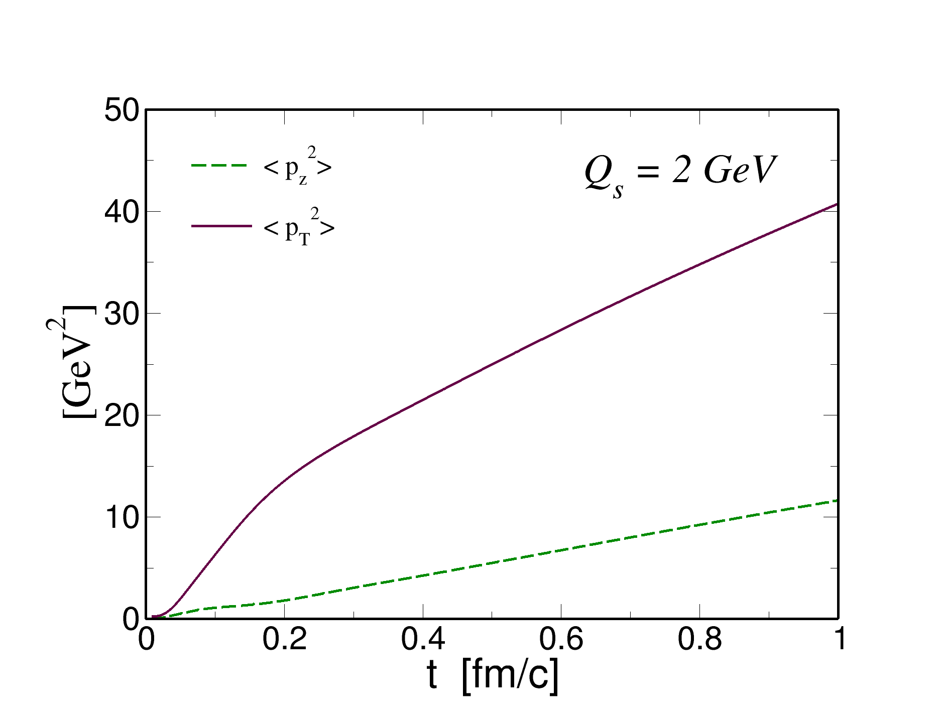
In Fig. 1 we plot the momentum broadening of HQs in the evolving Glasma fields: solid line denotes while dashed line stands for ; we remind that the direction coincides with the initial direction of the gluon fields in the Glasma (in realistic collisions, it is the flight direction of the two colliding objects). The initial condition corresponds to GeV, GeV and we checked that results are qualitatively unchanged for different initial momenta. We note that the momentum broadening is anisotropic: this is due to the anisotropy of the gluon fields [50, 56]. As we mentioned in the previous section, the anisotropic momentum broadening is vey important to generate anisotropic angular momentum fluctuations.
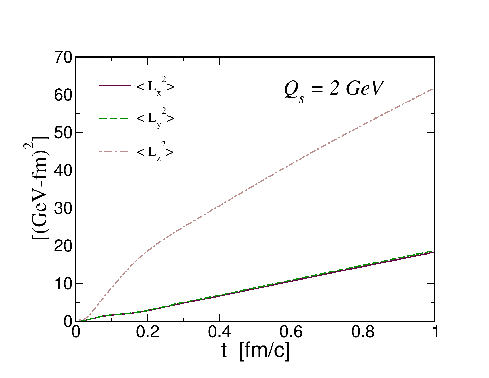
In Fig. 2, we plot the square of the components of the angular momentum, namely , and for GeV. For the system at hand during the entire evolution, therefore the quantities shown in Fig. 2 correspond to the spreading of the components of , similarly to the spreading of ordinary momentum studied in the theory of the Brownian motion, . We notice that . Hence, the interaction of HQs with the gluon fields produces anisotropic fluctuations of the angular momentum.
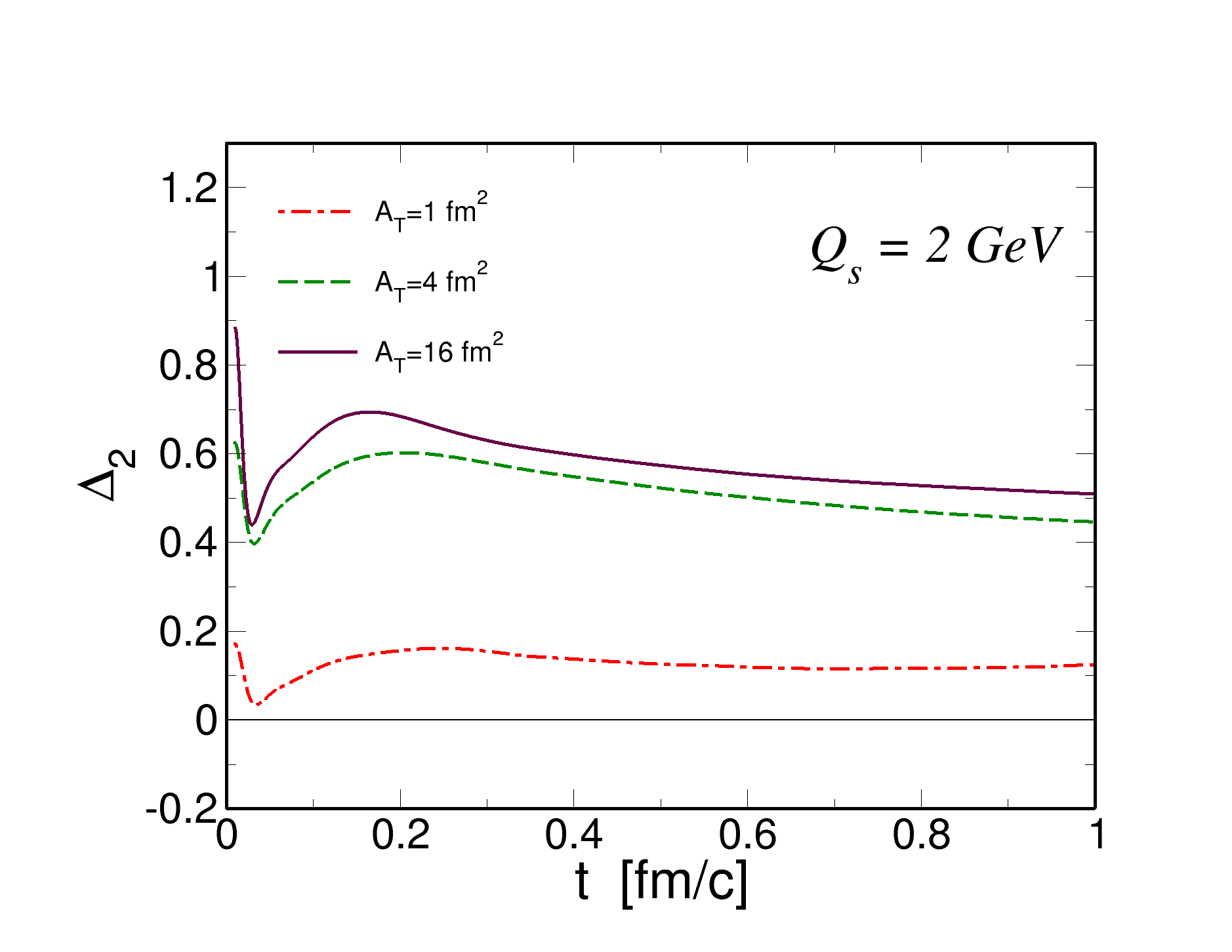
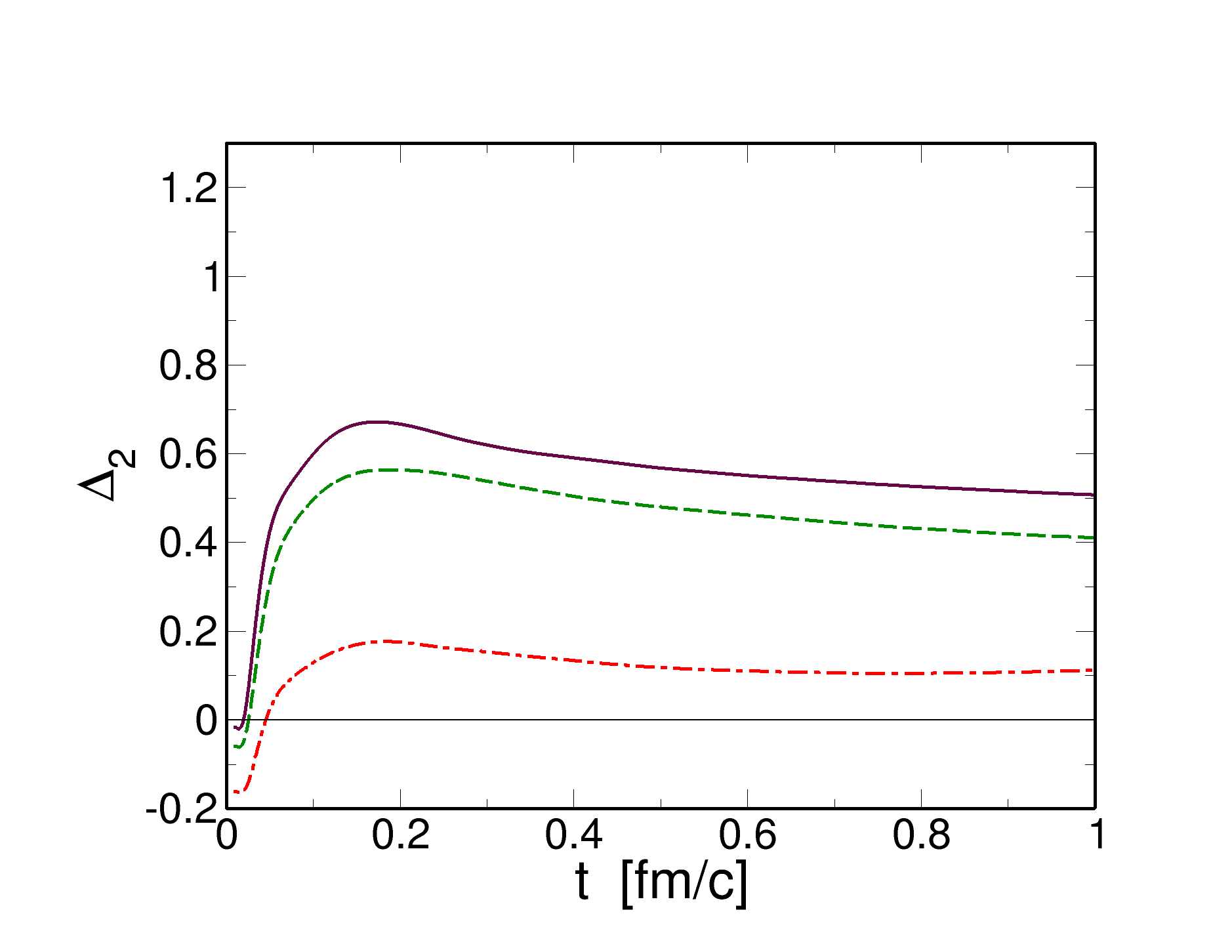
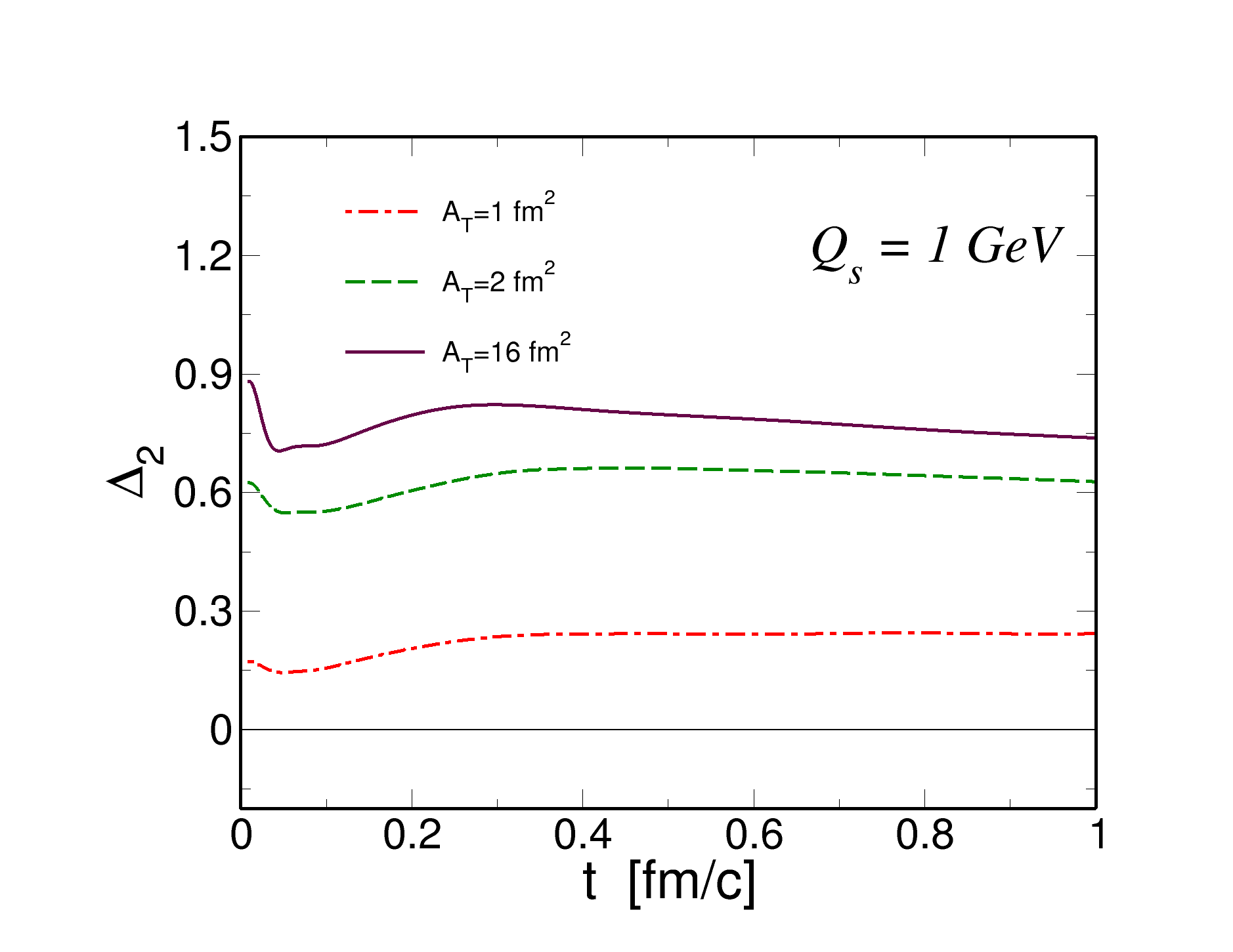
In Fig. 3 we plot versus time for several values of ; in the figure we defined the transverse area of the box, . We show results for fm ( fm2), fm ( fm2) and fm ( fm2). Calculations correspond to fm. Upper and lower panels correspond to the initializations GeV, and GeV, GeV respectively. The saturation scale is GeV. With the initialization for GeV we mean that GeV for and GeV for : it is done to mimic the central rapidity region of a collision.
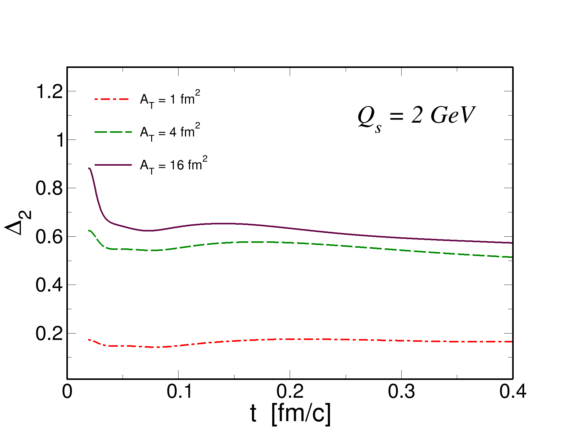
We note in Fig. 3 that in the case , besides a very quick transient, increases with time; within a time range that is relevant for realistic collisions, that is up to fm/c, the anisotropy of the fluctuations of lies within the and the in the cases of fm and fm respectively. Changing the initialization in simply changes a bit the short initial transient, but at regime the results of this case do not differ much with those obtained for . For fm remains smaller than the other two cases but it is still sizeable. We repeat this analysis (limited to the case ) for GeV and the result is shown in Fig. 4: we note that changing the does not lead to substantial changes of . We thus expect that even using a distribution in should not change too much the final value of .
We also note that the results shown in Fig. 3 are consistent with the discussion that lead to Eq. (42), namely that increasing the transverse size results in a which is almost independent on the size of the system. In fact, we note that while changing from fm to fm has a substantial effect on , doubling again to fm does not change significantly. We finally checked that changing the initial does not change qualitatively the results.
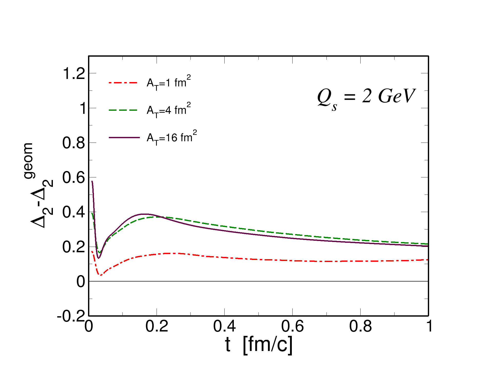
As discussed in the previous section, potentially takes contribution also from the anisotropic geometry of the fireball and would be nonzero even if the momentum broadening was isotropic. In order to prove that the results shown in Fig. 3 take a substantial contribution the anisotropic momentum broadening, we show in Fig. 5 for the few values of the transverse area already shown in Fig. 3, and is defined in Eq. (43). We note that is substantially different from , leading us to conclude that we show in Fig. 3 takes a concrete contribution from the anisotropy of the momentum broadening.
Although our calculations correspond to a large limit, we can check whether our results qualitatively (and to some extent, also quantitatively) stand for lower masses. To this end, in Fig. 6 we plot versus time for GeV that roughly corresponds to the mass of the beauty quark. We note that both qualitatively and quantitatively the agrees with that we found for a larger mass, suggesting that the anisotropy of the fluctuations of are quite robust.
As we discussed in the previous section, we do not consider spin fluctuations here because they are too small in magnitude compared to the fluctuations, and they remain isotropic. Moreover, fluctuations of and are uncorrelated (we confirmed this by direct calculations), therefore we can safely assume that the fluctuations of the total angular momentum, , are
| (45) |
As a consequence, defined in Eq. (40) represents also the anisotropy of the fluctuations of , hence our results predict anisotropic fluctuations for the total angular momentum of the HQs in the evolving Glasma fields.
IV Conclusions and outlook
We studied the fluctuations of angular momentum of very massive quarks in the pre-equilibrium stage of relativistic nuclear collisions, in the background of the evolving Glasma fields. The heavy quark mass is taken to be GeV, hence our model serves as a toy model of the heavy quarks (HQs), charm and beauty, produced in the collisions. We solved the non-relativistic kinetic equations in which the HQs diffuse in the background gluon fields; the evolution of the latters is obtained by solving the Yang-Mills equations with the Glasma initial condition. The implementation of the realistic HQs masses, namely charm and beauty, require the use of relativistic equations and these will be the subject of a future study.
We found that the fluctuations of the angular momentum, , of HQs are anisotropic, and we explained this in terms of the anisotropy of the gluon fields which in turn results in the anisotropic fluctuations of momentum. We introduced an anisotropy parameter, in Eq. (40), that measures the anisotropy of the fluctuations along the and directions and that we showed in Fig. 3. We found that the anisotropy develops quite early and can be as large as the for larger systems, remaining of about the for transverse areas of the order of the proton size. We checked that the qualitative picture is unchanged by changing the initialization in momentum space as well the value of the saturation scale, . Moreover, we computed the evolution of spin fluctuations but we found no sign of anisotropy in these fluctuations: it is likely that this happens as a combination of the random fluctuations of the color-magnetic fields as well as of the large value of (paramagnetic coupling is suppressed by a power of ).
Considering that the fluctuations of are way larger than those of , and that and are uncorrelated, we can safely assume that the fluctuations of the total angular momentum coincides with those of the components of , that is for . Therefore, the results of our study suggest that the fluctuations of the total angular momentum of HQs in the evolving Glasma fields are anisotropic.
We would like to stress that even though our results were obtained by using toy heavy quarks, we do not expect that the qualitative behavior of the quantities we computed will change when realistic quark masses will be implemented: as a matter of fact, the anisotropy of the fluctuations of the angular momentum depends on the structure of the gluon fields in the evolving Glasma and not on the value of the quark mass, therefore even lowering the value of the latter should not change drastically, or at least qualitatively, our results.
There are several ways in which this study can be improved. First of all, we would like to formulate the problem relativistically, in order to make calculations with the realistic values of the masses of charm and beauty quarks. The equations for this case already exist in the literature [58] and can be implemented within our scheme. Turning to the relativistic equations will also trigger interesting, purely relativistic effects [62] that might give correlations between and . In fact, within our scheme we already have a direct coupling of to , see Eq. (30), and hence to , but this coupling is suppressed by a power of the HQ mass and gives a negligible contribution to the evolution of the physical quantities: it is likely that in the relativistic calculation that term gives a sizeable effect. Moreover, in the relativistic case our Eq. (32) has to be replaced by a BMT-like equation [59, 58], in which the spin couples to the momentum as well as to the inhomogeneities of the gauge fields; in the full relativistic calculation this coupling, which is of the order of , would join the aforementioned couplings already present in the non-relativistic limit, and could also strengthen the correlation between and : as a result the anisotropy of the fluctuations of that we discussed could be transferred to the fluctuations of . In addition to this, it would be interesting to prepare a rapidity-dependent initialization of the gluon fields, similarly to what already done in relativistic hydrodynamics and kinetic theory [63, 64] that would allow us to have a nonzero average angular momentum of the bulk and of the HQs. Furthermore, in order to make more concrete phenomenological predictions, one should prepare a more realistic initial condition in which the fluctuates on the transverse plane, then attach the evolution of the HQs in the Glasma fields to that in the QGP droplets and eventually to hadronization: this is is quite an ambitious project and will be the subject of future studies.
Acknowledgements.
M.R. acknowledges John Petrucci for inspiration. Lucia Oliva is acknowledged for the numerous discussions on the topics of the research presented here. S.K.D. and M.R. acknowledge the support by the National Science Foundation of China (Grant Nos. 11805087 and 11875153). S.K.D. acknowledges the support from DAE-BRNS, India, Project No. 57/14/02/2021-BRNS.References
- [1] E. V. Shuryak, Nucl. Phys. A 750, 64-83 (2005)
- [2] B. V. Jacak and B. Muller, Science 337, 310-314 (2012)
- [3] L. D. McLerran and R. Venugopalan, Phys. Rev. D 49, 2233 (1994)
- [4] L. D. McLerran and R. Venugopalan, Phys. Rev. D 49, 3352 (1994)
- [5] L. D. McLerran and R. Venugopalan, Phys. Rev. D 50, 2225 (1994)
- [6] F. Gelis, E. Iancu, J. Jalilian-Marian and R. Venugopalan, Ann. Rev. Nucl. Part. Sci. 60, 463 (2010).
- [7] E. Iancu and R. Venugopalan, In *Hwa, R.C. (ed.) et al.: Quark gluon plasma* 249-3363.
- [8] L. McLerran, arXiv:0812.4989 [hep-ph]; hep-ph/0402137.
- [9] F. Gelis, Int. J. Mod. Phys. A 28, 1330001 (2013)
- [10] A. Kovner, L. D. McLerran and H. Weigert, Phys. Rev. D 52, 6231 (1995)
- [11] A. Kovner, L. D. McLerran and H. Weigert, Phys. Rev. D 52, 3809 (1995)
- [12] M. Gyulassy and L. D. McLerran, Phys. Rev. C 56, 2219 (1997)
- [13] T. Lappi and L. McLerran, Nucl. Phys. A 772, 200 (2006)
- [14] A. Krasnitz, Y. Nara and R. Venugopalan, Nucl. Phys. A 727, 427 (2003)
- [15] K. Fukushima, F. Gelis and L. McLerran, Nucl. Phys. A 786, 107 (2007)
- [16] H. Fujii, K. Fukushima and Y. Hidaka, Phys. Rev. C 79, 024909 (2009)
- [17] K. Fukushima, Phys. Rev. C 89, no. 2, 024907 (2014)
- [18] P. Romatschke and R. Venugopalan, Phys. Rev. Lett. 96, 062302 (2006)
- [19] P. Romatschke and R. Venugopalan, Phys. Rev. D 74, 045011 (2006)
- [20] K. Fukushima and F. Gelis, Nucl. Phys. A 874, 108 (2012).
- [21] F. Prino and R. Rapp, J. Phys. G 43, no. 9, 093002 (2016)
- [22] A. Andronic et al., Eur. Phys. J. C 76, no. 3, 107 (2016)
- [23] R. Rapp, P. B. Gossiaux, A. Andronic, R. Averbeck, S. Masciocchi, A. Beraudo, E. Bratkovskaya, P. Braun-Munzinger, S. Cao and A. Dainese, et al. Nucl. Phys. A 979 (2018), 21-86
- [24] S. Cao, G. Coci, S. K. Das, W. Ke, S. Y. F. Liu, S. Plumari, T. Song, Y. Xu, J. Aichelin and S. Bass, et al. Phys. Rev. C 99, no.5, 054907 (2019)
- [25] G. Aarts et al., Eur. Phys. J. A 53, no. 5, 93 (2017)
- [26] V. Greco, Nucl. Phys. A 967, 200 (2017).
- [27] X. Dong and V. Greco, Prog. Part. Nucl. Phys. 104 (2019), 97-141
- [28] Y. Xu, S. A. Bass, P. Moreau, T. Song, M. Nahrgang, E. Bratkovskaya, P. Gossiaux, J. Aichelin, S. Cao and V. Greco, et al. Phys. Rev. C 99 (2019) no.1, 014902
- [29] G. D. Moore and D. Teaney, Phys. Rev. C 71, 064904 (2005)
- [30] H. van Hees, V. Greco and R. Rapp, Phys. Rev. C 73, 034913 (2006)
- [31] H. van Hees, M. Mannarelli, V. Greco and R. Rapp, Phys. Rev. Lett. 100, 192301 (2008)
- [32] P. B. Gossiaux and J. Aichelin, Phys. Rev. C 78, 014904 (2008)
- [33] M. He, R. J. Fries and R. Rapp, Phys. Rev. C 86, 014903 (2012)
- [34] J. Prakash, M. Kurian, S. K. Das and V. Chandra, Phys. Rev. D 103 (2021) no.9, 094009
- [35] T. Song, H. Berrehrah, D. Cabrera, J. M. Torres-Rincon, L. Tolos, W. Cassing and E. Bratkovskaya, Phys. Rev. C 92, no. 1, 014910 (2015)
- [36] W. M. Alberico, A. Beraudo, A. De Pace, A. Molinari, M. Monteno, M. Nardi and F. Prino, Eur. Phys. J. C 71, 1666 (2011)
- [37] T. Lang, H. van Hees, J. Steinheimer, G. Inghirami and M. Bleicher, Phys. Rev. C 93, no. 1, 014901 (2016)
- [38] S. K. Das, F. Scardina, S. Plumari and V. Greco, Phys. Lett. B 747, 260 (2015)
- [39] Y. Xu, J. E. Bernhard, S. A. Bass, M. Nahrgang and S. Cao, Phys. Rev. C 97, no. 1, 014907 (2018)
- [40] S. Cao, T. Luo, G. Y. Qin and X. N. Wang, Phys. Rev. C 94, no. 1, 014909 (2016)
- [41] S. K. Das, S. Plumari, S. Chatterjee, J. Alam, F. Scardina and V. Greco, Phys. Lett. B 768, 260 (2017)
- [42] S. K. Das, M. Ruggieri, F. Scardina, S. Plumari and V. Greco, J. Phys. G 44, no. 9, 095102 (2017)
- [43] S. K. Das, M. Ruggieri, S. Mazumder, V. Greco and J. e. Alam, J. Phys. G 42, no. 9, 095108 (2015)
- [44] T. Song, P. Moreau, J. Aichelin and E. Bratkovskaya, Phys. Rev. C 101 (2020) no.4, 044901
- [45] A. Beraudo, A. De Pace, M. Monteno, M. Nardi and F. Prino, JHEP 1603, 123 (2016)
- [46] S. K. Das, F. Scardina, S. Plumari and V. Greco, Phys. Rev. C 90, 044901 (2014)
- [47] H. Berrehrah, E. Bratkovskaya, W. Cassing, P. B. Gossiaux, J. Aichelin and M. Bleicher, Phys. Rev. C 89, no.5, 054901 (2014)
- [48] F. Scardina, S. K. Das, V. Minissale, S. Plumari and V. Greco, Phys. Rev. C 96, no.4, 044905 (2017)
- [49] S. Mrowczynski, Eur. Phys. J. A 54, no. 3, 43 (2018)
- [50] M. Ruggieri and S. K. Das, Phys. Rev. D 98, no.9, 094024 (2018)
- [51] Y. Sun, G. Coci, S. K. Das, S. Plumari, M. Ruggieri and V. Greco, Phys. Lett. B 798, 134933 (2019)
- [52] J. H. Liu, S. Plumari, S. K. Das, V. Greco and M. Ruggieri, Phys. Rev. C 102, no.4, 044902 (2020)
- [53] K. Boguslavski, A. Kurkela, T. Lappi and J. Peuron,
- [54] J. H. Liu, S. K. Das, V. Greco and M. Ruggieri, Phys. Rev. D 103 (2021) no.3, 034029
- [55] P. Khowal, S. K. Das, L. Oliva and M. Ruggieri, Eur. Phys. J. Plus 137 (2022) no.3, 307
- [56] A. Ipp, D. I. Müller and D. Schuh, Phys. Lett. B 810, 135810 (2020)
- [57] T. Kunihiro, B. Muller, A. Ohnishi, A. Schafer, T. T. Takahashi and A. Yamamoto, Phys. Rev. D 82, 114015 (2010)
- [58] U. W. Heinz, Annals Phys. 161, 48 (1985)
- [59] V. Bargmann, L. Michel and V. L. Telegdi, Phys. Rev. Lett. 2, 435-436 (1959)
- [60] T. Lappi, Eur. Phys. J. C 55, 285-292 (2008)
- [61] M. Ruggieri, L. Oliva, G. X. Peng and V. Greco, Phys. Rev. D 97, no.7, 076004 (2018)
- [62] F. Becattini, [arXiv:2204.01144 [nucl-th]]. [63]
- [63] F. Becattini, G. Inghirami, V. Rolando, A. Beraudo, L. Del Zanna, A. De Pace, M. Nardi, G. Pagliara and V. Chandra, Eur. Phys. J. C 75, no.9, 406 (2015) [erratum: Eur. Phys. J. C 78, no.5, 354 (2018)]
- [64] L. Oliva, S. Plumari and V. Greco, JHEP 05, 034 (2021)