Liquid Democracy.
Two Experiments on Delegation in Voting

Abstract

Liquid Democracy is a voting system touted as the golden medium between representative and direct democracy: decisions are taken by referendum, but voters can delegate their votes as they wish. The outcome can be superior to simple majority voting, but even when experts are correctly identified, delegation must be used sparely. We ran two very different experiments: one follows a tightly controlled lab design; the second is a perceptual task run online where the precision of information is ambiguous. In both experiments, delegation rates are high, and Liquid Democracy underperforms both universal voting and the simpler option of allowing abstention.

JEL codes: C92, D70, D72, D83

Keywords: voting rules, majority voting, information aggregation, laboratory experiments, Condorcet Jury theorem, Random Dot Kinematogram.

1 Introduction

I believe that some sort of computerized participation by large numbers of the public in opinion formation and direct policy-making is in the cards in the next ten to twenty years. It may be that we will be able to turn this new technology to the improvement and defense of democratic institutions. I hope so. However, it is by no means evident that this will be the result. (Martin Shubik, 1970, commenting on Miller, 1969)

In Western societies, the sense of living in a crisis of traditional political institutions is bringing calls for different, more participatory forms of democracy. Among these, Liquid Democracy has caught the imagination of the young and the tech-savvy. It advocates a voting system where all decisions are submitted to referendum, but voters can delegate their votes freely. Beyond its intellectual roots in the writings of Charles Dodgson (in particular, Dodgson, 1884), Liquid Democracy was proposed more recently by James Miller in 1969. It has been adopted occasionally for internal decisions by European protest parties–the Swedish and the German Pirate parties being the most famous examples–and now finds vocal support in the tech community, where it aligns both with the emphasis on a non-hierarchical order and with the use of cryptographic tools to maintain confidentiality and reliability. Although the details vary, the common point of different implementations is the ease and specificity of delegation. Supporters herald it as the golden medium between representative and direct democracy: better than the former because representatives can be chosen according to their specific competence on each decision, better than the latter because uninformed or uninterested voters can delegate their votes.

There is a clear, immediate problem: are experts correctly identified? But there is also a second, more subtle, but also more fundamental question: even if the experts are correctly identified, delegation deprives the electorate of the richness of noisy but abundant information distributed among all voters. Unless the extent of delegation is modulated correctly, Condorcet has taught us that a smaller number of independent voters, even if more accurate, may well lead to worse decision-making. This very basic trade-off is the necessary point of departure of Liquid Democracy and is the focus of this paper.

We study a canonical common interest model where voters receive independent signals, conditional on an unknown state ex ante equally likely to take one of two values. The common objective is to identify the state correctly, aggregating information via majority voting. Signals vary across individuals in the probability of being correct—a variable we denote as precision. Experts are publicly identified and the precision of their signals is known; for all other voters, signals’ precisions are private information but known to be weakly lower than the experts’. If a voter chooses to delegate, the vote is randomly assigned to one of the experts. We begin by showing theoretically that for any size of the group and any number of experts, there is an equilibrium with positive delegation such that the outcome is superior to majority voting without delegation. However, in such an equilibrium delegation must not be too frequent, given its informational cost. The finding is not surprising, but the equilibrium frequency is counter-intuitively low. For example, consider one of the parametrizations we study: a group of 15 voters of which 3 are experts; the experts’ information is correct with probability 70%, while the precision of non-experts’ signals can take any value between 50 and 70%, with equal probability. Then only non-experts with signals of precision close to random should delegate: a non-expert with information that she knows is only 55% likely to be correct should not delegate to experts whom she knows to be correct with probability 70%. And mistakes are costly: small errors towards over-delegation lead to expected losses that soon become severe. In actual implementations, other factors, for example overconfidence and overweighing of own information, could introduce countervailing forces. It is with these concerns in mind that we test Liquid Democracy with two very different experimental designs.

Before describing the experiments in detail, note that the informational benefit from overweighing voters with more precise signals can be achieved via abstention as well, as long as abstention correlates with less accurate signals. Abstention differs from delegation because the increase in voting weight concerns all individuals who choose to vote, not only those targeted as delegates. Yet, we know from McMurray (2013) that, under common interest and in the absence of voting costs, it too can lead to improvements over simple majority voting, and for reasons very similar to those favoring delegation. Abstention is a familiar option and does not require any transfer of votes, reducing the appearance of suspicious deals. Its performance relative to delegation is thus an interesting question per se, and our experiments compare the two alternatives.

The first experiment was designed for the lab and follows the theory very closely. We study groups of either 5 voters (of which 1 is an expert) or 15 voters (of which 3 are experts). We observe the frequency of delegation and the fraction of group decisions that yield the correct outcome. We then compare these results to a second treatment, where the option of abstention takes the place of delegation. Finally, we evaluate both treatments relative to simple majority voting with voting by all. We find systematic over-delegation: delegation rates that are between two and three times the rate in the unique strict equilibrium, given the realized experimental precisions. As a result, Liquid Democracy (LD) underperforms, relative to simple majority voting without delegation. Under Majority Voting with Abstention (MVA), abstention rates are instead very close to the theory, and the fraction of correct decisions is comparable to what majority voting without abstention (or delegation) would deliver. Interestingly, MVA suffers from its own sub-optimal behavior: in our symmetric environment, voting in line with one’s own signal is optimal, but experimental subjects occasionally deviate, and deviate more when abstention is allowed. In the data, voting according to signal correlates positively with the signal’s precision, and since more subjects vote under abstention, at lower precisions, we also observe more votes against signal. Although the frequency of such deviations remains low, the result is a decline in correct group decisions that prevents MVA from reaping the gains over universal voting that theory predicts. The conclusion of our first experiment, then, is that even when experts are correctly identified and both LD and MVA have the potential to dominate universal majority voting, both systems in fact fail to do so. LD in particular shows a more clearly detectable negative effect.

The experimental design we implemented is canonical: it follows standard procedures for voting experiments with common values and has been widely and successfully used in the literature (for example, Guarnaschelli et al., 2000; Battaglini et al., 2010; Goeree and Yariv, 2011). But could the design itself be biasing results against LD and MVA? There are three reasons to consider the question. First, as mentioned, the theoretical thresholds for equilibrium delegation seem counter-intuitive. But what makes them counter-intuitive, in our view, is not their low value per se but the detailed mathematical manner in which information is conveyed in the experiment. Each participant is told a number for her own precision and is naturally induced to compare such number to the known precision of the experts–in the earlier example, the fact that 55% is transparently lower than 70% makes the difference very salient. In reality, voting decisions take place in an ambiguous world, where individuals do not have explicit numerical knowledge of the reliability of their and others’ information. Evaluations are fuzzier. Second, and related, a similar argument may affect voting against signal under MVA. The detailed mathematical design gives us clean theoretical predictions, but could in fact be confusing participants, no matter how much we clarify the instructions. At 55% precision, thinking that one should vote against signal about half the time is a reasonable enough thought. In an actual voting situation, however, lacking an explicit mathematical value for the probability that one’s information is correct, it is unlikely that individuals would vote against their best estimate of the right decision.

Finally, there is a third reason for considering a less controlled environment. Could our detailed mathematical design be favoring universal majority voting? In a still current analysis of the Condorcet Jury theorem, suggestively titled “A Note on Incompetence,” Margolis (1976) discussed the tension between the asymptotic efficiency promised by the theorem and political reality. The existence of private interests, correlated signals, and asymmetric scenarios all may lead direct democracy to function less well, but Margolis proposed a different explanation. What if, over some questions and for some voters, information is actually correct with probability lower than $1/2$? For any individual voter this will not be true when averaging over many decisions, but may well be true over some. And it will affect the probability that the majority decision is correct. By opening some space for improvement over universal majority voting, note also that the possibility of worse than random information allows testing LD in larger electorates, where it is meant to be applied, while maintaining pure common interest and independent signals. We see this as an additional argument for a less mathematically precise environment.

Our second experiment then is meant to capture a voting environment where voters have “some sense” of how well-informed they are and how likely they are to be correct, and similarly of how likely experts are to be correct, but such sense is vague and instinctive. There is of course a cost: we lose the precise control granted by Experiment 1. However, even though our aims are different, we can exploit a very rich literature that studies problems with exactly these features: the large literature in psychology and neuroscience that studies perceptual tasks. Our focus is not on measuring accuracy of perception, but on designing the task as a group decision problem.

The Random Dot Kinematogram (RDK) is a classic perceptual task amply used in vision and cognitive research. A number of moving dots are displayed for a very short interval; some move in a coherent direction, either Left or Right in our binary implementation, others move at random; subjects report in which direction they think coherent dots are moving. We can label experts ex post as the individuals with performance in the highest quintile, and generate a collective decision by aggregating individual responses, with the additional option of delegation to the experts (in the LD treatments) or abstention (in the MVA treatments). We ran the experiment on Amazon Mechanical Turk with three electorate sizes: $N=5$ and $N=15$, as in Experiment 1, and a larger electorate of $N=125$.

We reach three results. First, in our experiment it is not rare for individuals’ accuracies to be worse than random. And this even over a large number of decisions: aggregating at the subject level over all 120 tasks, around 10% of subjects have ex post accuracy strictly below randomness; about 15% do no better than randomness. If we want to study voting and information aggregation when information may be faulty, perceptual tasks can provide a very useful tool.

Second, comparing delegation to abstention we find the same patterns we saw in Experiment 1. The distributions of voters’ accuracies we observe in the two samples—LD and MVA—are effectively identical, but delegation is twice as frequent than abstention when $N=5$, and more than 50% more frequent when $N=15$, if anything accentuating the disparity observed in the first experiment. Between one fourth and one third of subjects choose to abstain, but about half, in all treatments, choose to delegate.

Third, the high frequency of delegation exacts its expected informational costs. Even with a relatively high fraction of random, or below random subjects, universal majority voting remains the best information aggregator, delivering the highest frequency of correct group decisions in all treatments; MVA is only slightly less efficient, while LD is dominated by both in all treatments.

The main contribution of this study is the robustness of the conclusions across two very different experimental designs. The second design sacrifices experimental control in exchange for a less mathematical formulation; it conveys less information to the subjects and leaves more space for idiosyncratic responses; it is run on MTurkers rather than students, it is much shorter, and it includes one treatment with a much larger group. And yet, and contrary to our expectations, treatment effects in the second design closely replicate the effects we observe in the first. In a pure common interest setting where experts are correctly identified, individuals over-delegate. The resulting increase in the voting weight of the experts does not lead to an increase in efficiency because the extent of delegation is too high, and thus the net informational effect is negative. Experimental subjects are less prone to abstaining, and thus the simpler routine option of allowing abstention leads to better outcomes than allowing delegation.

The second contribution of this study is methodological. While the controlled design of our first experiment in the end delivers robust conclusions, we think that it is important to add to our experimental tool-kit designs that recognize the ambiguity present in group decision-making. Experiments on ambiguity at the individual level are common; to our knowledge they are much less so for collective decision-making. In voting problems, in particular, the complexity of many questions and the imbalance between the cost of acquiring information and the small marginal impact of a single vote make the lack of precise information very likely. Perceptual tasks, with the large and sophisticated literature that accompanies them, can be a particularly usable tool. In this study, it is the combination of a strictly controlled design in the lab with the freer design of the perceptual task that teaches us the most.

Our work is related to three separate literatures. First, to the study of voting as information aggregation. The informational costs and benefits of delegating to better informed individuals in pure common interest voting problems were the subject of early studies on the Condorcet Jury theorem (Margolis, 1976; Grofman et al., 1983; Shapley and Grofman, 1984), highlighting, as we do, the trade-off between the loss in aggregate information and the more precise information of the experts. These studies asked important statistical questions but did not focus on rational equilibrium behavior. More recent work (Austen-Smith and Banks, 1996; Feddersen and Pesendorfer, 1997; McLennan, 1998; Wit, 1998) put the analysis of the Condorcet Jury theorem on solid equilibrium grounds, but abstracted from the focus on delegation. We did not find in the literature our starting theoretical result—in a finite sample, the efficient equilibrium must allow for delegation—but the result builds on the work of McLennan. As we discussed, the trade-off identified in the case of delegation exists also in the case of abstention. Here the best-known work includes partisan voters (Feddersen and Pesendorfer, 1996), but the analysis can also be profitable and rich in a pure common interest setting, as shown by Morton and Tyran (2011) in the case of three voters, and more generally by McMurray (2013). Battaglini et al. (2010) and Morton and Tyran (2011) test the theoretical predictions in the lab. Morton and Tyran’s model is close to ours, and, contrary to Battaglini et al., allows for a range of information types and does not rely on the existence of perfectly informed voters. Interestingly, Morton and Tyran find that experimental subjects appear predisposed towards abstaining, doing so even when abstention is dominated. In their words, subjects “follow a norm of “letting the experts decide.”” According to our experimental results, this tendency is strengthened further when the choice is explicitly phrased as delegation. We are not aware of experimental works that study delegation in voting as tool for information aggregation.

The second strand of related works are studies of Liquid Democracy. Most belong either in normative political theory or in computer science. Green-Armytage (2015) and Blum and Zuber (2016) discuss what they see as normative advantages of Liquid Democracy, on both epistemic and equalitarian reasons: decisions are taken by better informed voters, and at the same time LD avoids the creation of a detached class of semi-permanent professional representatives. Because the focus is normative, these studies do not analyze strategic incentives. The computer science literature is instead largely concerned with understanding how LD would work in practice. It models behavior via a priori algorithms and studies rich interactions where delegation takes place on networks (Christoff and Grossi, 2017; Kahng, Mackenzie and Procaccia, 2018; Bloembergen, Grossi and Lackner, 2019; Caragiannis and Michas, 2019). These authors connect LD to the social choice tradition, but here too strategic considerations are absent. An exception is Armstrong and Larson (2021) which discusses the informational trade-off involved in delegation and focuses on a Nash equilibrium. The paper retains the algorithmic flavor of this literature by modeling the delegation choice as sequential; the common interest nature of the problem, together with the added assumptions of complete information and costly voting, then results in the equilibrium superiority of delegation over universal majority voting. The theoretical conclusion is thus similar to ours, but the model and the assumptions driving the result differ. Strategic concerns are at the heart of two recent paper in economics, Ravindran (2021) and Dhillon et al. (2021). In Ravindran’s model, voters’ types are binary and known, with either high or low information accuracy, and the goal is the characterization of the efficient equilibrium. With a single expert, optimal delegation is defined precisely; with multiple experts, complications can arise although, as in Armstrong and Larson, they can be solved if delegation decisions are sequential. Dhillon et al. study delegation in a model à la Feddersen and Pesendorfer (1996), with partisan voters and perfectly informed experts. As in the papers just discussed, they show that under complete information delegation has desirable properties: the game is dominance-solvable and delegation allows voters to coordinate on the best equilibrium. With incomplete information, multiple equilibria are more difficult to avoid and results are weaker. None of these works is experimental.

Finally, a literature in social psychology studies a question that is closely related to our second experiment: if a group of individuals face, individually, a perceptual task but can then aggregate their reactions into a group decision, which decision rule for the group will reach the correct answer most frequently? How does simple majority rule compare to supermajority thresholds? In Sorkin et al. (1998), a small group of subjects are faced with a signal detection task and asked whether the display reflects noise only or signal plus noise. Although the group falls short of normative predictions, simple majority rule leads to the highest accuracy. Individual behavior is modeled as reflecting two main parameters, detection sensitivity and confidence, and the emphasis on confidence shapes the direction this research has since taken. In small groups, decision typically follows discussion, and during discussion individual confidence translates into influence. Communication thus threatens group accuracy, unless confidence correlates positively with individual sensitivity (Sorkin et al., 2001; Bahrami et al., 2012; Silver et al., 2021). Although it seems a natural next step, we are not aware of similar studies that include the possibility of delegation.

In what follows, we begin by describing the theoretical model (Section 2) and its equilibrium properties (Section 3). We then discuss our first experiment: its parametrization and treatments (Section 4); its implementation (Section 5), and its results (Section 6). Section 7 describes the motivation and the design of our second experiment; Section 8 reports its results. Section 9 concludes. The Appendix collects longer proofs and some additional experimental findings.

2 The Model

We study the canonical problem of information aggregation through voting in a pure common interest problem. $N$ (odd) voters face an uncertain state of the world $\omega$ and must take a decision $d$. There are two possible states of the world, $\omega\in\{\omega_{1},\omega_{2}\}$, and two alternative decisions $d\in\{d_{1},d_{2}\}$. Every voter $i$’s payoff equals 1 if the decision matches the state of the world ($d=d_{s}$ when $\omega=\omega_{s},s=1,2$), and 0 otherwise. Voters share a common prior $\pi=Pr(\omega_{1})$ and receive conditionally independent signals $\sigma_{i}\in\{\sigma_{1},\sigma_{2}\}$ that recommend one of the two decisions. We call $q_{i}$ the precision of individual $i$’s signal, or the probability that $i$’s signal is correct. Precision varies across individuals but is symmetric over the two possible states of the world: $q_{i}=Pr(\sigma_{i}=\sigma_{1}|\omega_{1})=Pr(\sigma_{i}=\sigma_{2}|\omega_{2})$.

The group of $N$ voters is composed of $K$ (odd) experts and $M$ (even) non-experts. Whether any given voter is an expert or a non-expert is commonly known. Every expert $e$ receives signals of known precision $q_{e}=p$. The precision of a non-expert $i$’s signal is instead private information: $q_{i}$ is an independent draw from a commonly known distribution $F(q)$ everywhere continuous over support $[\underline{q},\overline{q}]$ , with $\underline{q}=1/2$ and $\overline{q}=p$. The signals themselves are also private information, for both experts and non-experts. Each voter, whether expert or non-expert, holds a single non-divisible vote. We denote by $EU$ individual ex ante expected payoff, before the realizations of precisions and signals. $EU$ equals the ex ante probability that the group reaches the correct decision.

Before the election, each voter receives a signal and is informed of the signal’s precision. The voter then chooses whether indeed to vote, for one or the other of the two options, or whether to delegate the vote, and in this case, whether to delegate it to an expert or to a non-expert. If delegated, the vote is assigned randomly, with equal probability, to any individual in the indicated category. When counting votes, each voter who has chosen not to delegate receives a weight equal to the number of votes delegated to her, plus 1. The decision receiving more votes is chosen.

With an eye to the experimental implementation, we will select equilibria that require little coordination, and in particular such that experts never delegate, and non-experts only delegate to experts. Hence, multi-step delegation (i delegates to j who delegates to z) will not be observed in equilibrium, and thus neither will circular delegation flows (i delegates to j who delegates to z who delegates to i). The model nevertheless needs to specify what would happen in such cases. We allow for multi-step delegation: if delegation targets a voter who has herself chosen delegation, the full packet of votes is delegated according to her instructions. However, if a set of delegation decisions results in a circular delegation flow, we specify that one link in the cycle is chosen randomly and that delegation is redirected randomly to another voter in the selected category.

3 Equilibrium

We study an environment that matches the experimental set-up, and where, specifically, $\pi=Pr(\omega_{1})=1/2$. In this symmetric environment, conditional on voting, voting according to signal is an undominated strategy—a result that holds whether delegation is allowed, as in our model, or is not, as in traditional majority voting. Keeping in mind the experimental goal of the study, we focus on equilibria that require minimal coordination and in particular where the delegation decision depends on the signal’s precision, but not on its message. Thus, we select semi-symmetric Perfect Bayesian equilibria in undominated strategies where, when voting, voters follow their signal, and voters of a given type (non-experts or experts) follow the same strategy, symmetric across signals. In what follows, “equilibrium” refers to such a notion. We are interested in the welfare properties of delegation, and say that an equilibrium “strictly improves over majority voting” if in equilibrium the ex ante probability of reaching the decision that matches the state of the world is strictly higher than under (sincere) majority voting (MV), or $EU_{LD}>EU_{MV}$. Our most general theoretical result is summarized in the following theorem:

Theorem.

Suppose $\pi=Pr(\omega_{1})=1/2$. Then for any $F$ and for any $N$ and $K$ odd and finite there exists an equilibrium with delegation that strictly improves over MV.

The result is interesting because the environment we are studying is particularly favorable to MV. Given the symmetric prior and information structure, the Condorcet Jury theorem applies to rational voting, and thus we know that with voters voting sincerely MV converges to the correct decision with probability 1 asymptotically, as the size of the electorate becomes unbounded. In addition, we are restricting our attention to semi-symmetric equilibria under LD, and thus excluding asymmetric profiles of strategies that we know are efficient but that require demanding coordination. And yet, the theorem states that with a finite electorate there always exists an equilibrium where the possibility of delegation strictly improves over MV.

We prove the theorem in the Appendix, but the intuition is both straightforward and interesting. The essence of the proof is that, when delegation is possible and some voters’ information may be barely better than random, there cannot be an equilibrium where delegation is excluded with probability 1: every voter casting their vote with probability 1 (and thus replicating MV) is not an equilibrium. But in this common interest problem, we know from McLennan (1998) that if a set of strategies that maximizes expected utility exists, then it must be an equilibrium. We show in the Appendix that such a set does exist in our game, and thus an equilibrium must exist that strictly improves over MV. Finally, because the environment is fully symmetric for all voters of a given type, the conclusion continues to apply when we restrict attention to semi-symmetric strategies, and because semi-symmetric strategies that do not include delegation are inferior to MV with votes cast according to signal, the superior equilibrium must involve delegation.

The theorem does not characterize the equilibria with delegation. We do so in Section 4, when we specialize the model to the parameter values we use in the experiment. Here, to make sure the mechanisms that drive the model are intuitively clear, we describe in detail a semi-symmetric interior equilibrium for the case of a single expert.

3.1 A Single Expert ($K=1$)

Proposition 1.

Suppose $\pi=Pr(\omega_{1})=1/2$ and $K=1$. Then for any $N$ odd and finite, there exists an equilibrium such that: (i) the expert never delegates her vote and always votes according to signal; (ii) there exists a threshold $\widetilde{q}(N)\in$$(\underline{q},\overline{q})$ such that non-expert $i$ delegates her vote to the expert if $q_{i}<\widetilde{q}$ and votes according to signal otherwise. Such an equilibrium strictly improves over MV and is ex ante maximal among sincere semi-symmetric equilibria where the expert never delegates and non-experts delegate to the expert only.

The proposition is proved in the Appendix. The structure of the equilibrium, however, is intuitive. Note that in all interior equilibria (in fact, for any number of experts), non-experts must adopt monotone threshold strategies–there must exist a precision threshold $\widetilde{q}$ such that voters with lower precision delegate, and voters with higher precision do not. The reason is immediate: if the voter delegates, expected utility does not depend on the voter’s precision. But if the voter does not delegate, there is a non-zero probability that the voter is pivotal, in which case expected utility increases with the voter’s precision. The conclusion then follows. Given monotone threshold strategies, the Appendix shows that the delegation directions in the proposition – the expert never delegating and non-experts delegating to the expert only – are indeed best responses when all others adopt them too. And since we know, from the earlier theorem, that an equilibrium with partial delegation must exist, it follows that an equilibrium with the strategies characterized in the proposition must exist. Finally, we also find that the condition identifying the equilibrium threshold corresponds to the first order condition from the maximization of ex ante expected utility, over all profiles of semi-symmetric monotone threshold strategies with sincere voting and the specified directions of delegation. Hence, again invoking the theorem, the equilibrium is maximal over such profiles and improves strictly over majority voting.

It is important to note that the equilibrium threshold $\widetilde{q}$ that supports the improvement over MV is strictly interior to the range $(\underline{q},\overline{q})$. Because $\overline{q}=p$, that means that in equilibrium there are voters who know that their precision is strictly lower than the expert’s precision, and yet cast their vote, rather than delegating. Since delegation decreases the aggregate information in the system, and yet the equilibrium with delegation is superior to MV, we expect the threshold $\widetilde{q}$ to be low–only voters with very imprecise information delegate in equilibrium. Indeed, this is what the numerical examples will show. Studying in detail a particularly simple example makes clear why

Suppose $N=3$ and $K=1$, and consider non-expert $i$’s choice of whether or not to delegate to the expert. Note that $i$’s choice matters only if (a) $i$ ’s signal disagrees with the expert’s; (b) the other non-expert, $j$, does not delegate, and (c) $j$’s signal disagrees with the expert’s. Thus $i$ conditions on $j$ voting and receiving a signal that agrees with $i$’s own signal. Non-expert $i$ is indifferent between delegating and voting when $q(i)=\widetilde{q}$. Denoting by $\mu_{v}(\widetilde{q})=E(q|q>\widetilde{q})$ the expected precision of $j$’s signal, conditional on $j$ voting, equilibrium $\widetilde{q}$ thus solves:

$$p(1-\widetilde{q})(1-\mu_{v}(\widetilde{q}))=(1-p)\widetilde{q}\mu_{v}(\widetilde{q})$$

The equilibrium condition equalizes the probability that the expert is correct and both non-experts are not, with the probability that the expert is incorrect and both non-experts are correct. The non-expert signal with precision $\widetilde{q}$ receives implicit validation from a second independent and more accurate signal. It is this implicit validation that pushes equilibrium behavior away from delegation, and the equilibrium $\widetilde{q}$ towards low values. For example, with $N=3$ and $K=1$, if $p=0.7$ and $F(q)$ is Uniform over $[0.5,0.7]$, $\widetilde{q}=0.572$, below the mean non-expert precision of $0.6$. A non-expert voter’s precision is always lower than the expert’s, but the ex ante individual probability of delegation is only 36 percent.

The good properties of the equilibrium with $\widetilde{q}\in(\underline{q},\overline{q})$ depend strongly on the optimal, spare use of delegation. But internalizing such reasoning is difficult. Our first experiment tests participants’ behavior in an environment that mirrors the model closely.

4 Experiment 1: Treatments and Parametrizations

The game we study in Experiment 1 follows very closely the theoretical model, with one simplification. We constrain the direction of delegation: experts cannot delegate, and non-experts can only delegate to the experts. We are interested in three main questions: (1) We consider first the simplest setting, when decisions are taken by a small group and a single expert. How well does LD perform, relative to MV? (2) According to the theorem, LD’s potential to improve over MV persists with larger group sizes and multiple experts. In the lab, do results change qualitatively when the size of the group and the number of experts increase? (3) LD makes it possible to shift voting weight away from less informed voters and towards more informed ones. But reducing the weight of less informed voters can also be achieved, more simply, by allowing abstention. How does LD compare to MV with abstention? We denote such a rule by MVA, and as in the case of LD, study it both in a small group with a single expert, and in a larger group with multiple experts.

In all experiments, we set $p=0.7$, and $F(q)$ Uniform over $[0.5,0.7]$. We study four treatments. Two treatments concern LD. In LD1, groups consist of $5$ voters with a single expert: $N=5$, $K=1$. In LD3, each group has 15 voters in all, of which 3 are experts: $N=15$, $K=3$. Hence in both treatments one fifth of the group are experts: $K/N=1/5$. The two treatments with abstention, MVA1 and MVA3, substitute abstention for the possibility of delegation, again either with $N=5$, $K=1$ (MVA1), or with $N=15$, $K=3$ (MVA3).

4.1 Liquid Democracy

Table 1 reports the theoretical predictions when delegation is possible.

Table 1: $p=0.7$, $F(q)$ Uniform over $[0.5,0.7]$

$LD1:$ $N=5;$ $K=1$								$LD3:$ $N=15;$ $K=3$
$\widetilde{q}$	$F(\widetilde{q})$	$EU_{LD}$	$EU_{MV}$					$\widetilde{q}$3	$F(\widetilde{q}^{3})$	$EU_{LD}^{3}$	$EU_{MV}^{3}$
0.7	1	0.7	0.717					0.532	0.162	0.843	0.832
0.543	0.215	0.731

In treatment LD1, we find two semi-symmetric equilibria. For any realization of non-expert precisions, there always exists an equilibrium where every voter delegates to the expert with probability 1: no individual non-expert is ever pivotal, and delegating one’s vote is a (weak) best response. The expert then alone controls the outcome. With semi-symmetric strategies, such an equilibrium corresponds to $\widetilde{q}=\overline{q}$ and yields ex ante utility $EU_{LD}(\widetilde{q}=\overline{q})=p=0.7$. Note that such an equilibrium is not strict. In addition, there is a unique strict equilibrium where $\widetilde{q}$ is strictly interior. As argued earlier, the $\widetilde{q}$ threshold is low, and the ex ante probability of delegation is only just above 20 percent. The ex ante probability of reaching the correct decision, equivalent to the expected utility measures, is lowest when the expert decides alone $(\widetilde{q}=\overline{q})$, intermediate under $MV$, and highest in the equilibrium with delegation and interior $\widetilde{q}$. However, the proportional increase in the probability that the group selects the correct option is small, about 2 percent at each step.

In LD3, full delegation is not an equilibrium any longer. Intuitively, when there are multiple experts and all other non-experts delegate, voter $i$ can be pivotal only if the experts disagree among themselves. The disagreement reduces the attraction of delegation and for sufficiently high $q$ (still smaller than $\overline{q}$) casting a vote is preferable. As we know, the equilibrium with interior $\widetilde{q}$ continues to exist. Equilibrium delegation, however, is rare: the expected frequency of individual delegation falls to 16 percent. As theory teaches, the interior equilibrium yields a higher probability of a correct decision than MV. However, with the increase in the size of the group, the Condorcet Jury Theorem effect becomes very pronounced: majority voting works very well and the scope for improvement is small. The percentage gain is only 1.3 percent.

The table conveys two main messages. First, we see concretely what the interior equilibrium entails for the experimental parametrizations. In particular, as expected, equilibrium delegation is not frequent and concerns only voters with precisions not far from 0.5. Second, the improvement in the probability of making the correct decision is small, too small to be detectable in the lab. Setting a higher $p$, and/or setting $\overline{q}<p$ would increase the scope and expected gain from delegation; increasing $\underline{q}$ or $N$ would have the opposite effect. We have chosen a parametrization that delivers similar efficiencies for LD and for MV, and leave the data free to favor either. The realistic challenge for the experiment will be to see whether indeed in this environment the two systems are comparable.

4.2 Abstention

Like delegation, abstention can lower the voting weights of less informed voters, with the major advantage of being a simpler and familiar option. However, the two mechanisms are not equivalent: under abstention, voting weight is redistributed towards all voters who choose to vote; under LD, delegated votes target the experts only.

We implement the MVA treatments in the identical environment we study under LD. After non-expert voters learn, privately, the precision and the content of their personal signal, they decide, simultaneously and independently, whether to vote or to abstain. Experts are not given the option of abstaining. Everything else remains unchanged. The model of abstention is closely related to McMurray (2013), and its main results—the existence of an equilibrium in monotone cutpoint strategies, and its superiority to MV—carry over to our setting. We report the relevant equations in the Appendix. As in the case of delegation, and for very similar reasons, abstention too is limited to voters with weak information.

Table 2 shows the equilibria with abstention, for the experimental parametrizations. We denote by $\widetilde{\alpha}$ the precision threshold below which in equilibrium a non-expert abstains, and above which a non-expert votes.

Table 2: $p=0.7$, $F(q)$ Uniform over $[0.5,0.7]$

$MVA1:$ $N=5;$$K=1$								$MVA3:$ $N=15;$$K=3$
$\widetilde{\alpha}$	$F(\widetilde{\alpha})$	$EU_{MVA}$	$EU_{MV}$					$\widetilde{\alpha}$3	$F(\widetilde{\alpha}^{3})$	$EU_{MVA}^{3}$	$EU_{MV}^{3}$
0.7	1	0.7	0.717					0.7	1	0.784	0.832
0.580	0.40	0.724						0.580	0.40	0.849
0.5	0	0.717						0.5	0	0.832

For both group sizes, there are three semi-symmetric equilibria. Two are boundary equilibria, with either zero ($\widetilde{\alpha}=0.5)$ or full ($\widetilde{\alpha}=0.7$) abstention; one is an interior equilibrium where, for both group sizes, a non-expert abstains if precision is below 0.58, i.e. with ex ante probability of 40 percent. The boundary equilibrium with zero abstention corresponds to MV; the one with full abstention, where the decision is delegated to the experts, is inferior to MV. As in McMurray’s analysis, the interior equilibrium does deliver expected gains over MV, but these remain quantitatively small. The interior equilibrium threshold for abstention is higher than the threshold for delegation, and remains constant in the two group sizes. It implies a larger expected number of abstentions than delegations: for example, and rounding up to integers, when $N=15\text{,}$ in equilibrium we expect 2 non-experts to delegate under LD, but 5 non-experts to abstain under MVA.

Under both LD and MVA, the expected improvements over MV are minor. It is natural to ask how sensitive such potential improvements are to strategic mistakes.

4.3 Robustness

We consider here a particularly simple parametrization of strategic mistakes: we suppose that behavior remains symmetric, but the precision threshold for delegation or abstention is chosen incorrectly. In Figure 1, the horizontal axis is the common threshold, and the vertical axis reports gains and losses in expected utilities relative to MV (fixed at 1). Thus the plots depict the percentage changes in the probability of the group making the correct choice, relative to MV, at different delegation (abstention) thresholds. LD is plotted in blue; MVA in green; the first panel corresponds to $N=5$, $K=1$; the second to $N=15$, $K=3$. The highest points on the blue and green curves coincide with the respective equilibrium thresholds.

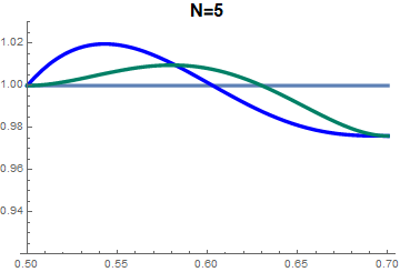
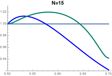
Figure 1: Robustness to strategic errors. The horizontal axis is $\widetilde{q}$ ($\widetilde{\alpha}$), the vertical axis is the probability of reaching the correct decision, relative to MV. blue is LD, green is MVA, and Grey is MV.

At $\widetilde{q}$ or $\widetilde{\alpha}=1/2$, no-one delegates their vote or abstains, and all curves equal MV and coincide. At $\widetilde{q}$ or $\widetilde{\alpha}=0.7$, all non-experts delegate or abstain, and only the expert/s decide(s). In the first panel, with a small group, the maximum potential improvement over MV from delegation (from LD) is higher than from abstention (MVA). However, this is not true in the second panel, with the larger group. Both results were already shown in Tables 1 and 2. More interesting is the range of thresholds for which each voting rule dominates MV. Here the message is consistent across the two group sizes: in both cases, the range of thresholds that deliver improvements over MV is limited, and particularly limited for LD. When the group is larger, LD’s potential for losses is evident in the figure, as is its increased fragility, relative to MVA: the range of thresholds that improve over MV is half as large under LD3 than under MVA3. With both voting schemes, but with LD in particular, while potential gains are small, there is the real danger of reaching worse decisions: under LD3, maximal potential losses are more than six times maximal potential gains.

5 Experiment 1: Implementation

We ran the experiment online over the Summer of 2021, using the Zoom videoconferencing software. Participants were recruited from the Columbia Experimental Laboratory for the Social Sciences (CELSS)’ ORSEE website. They received instructions and communicated with the experimenters via Zoom, and accessed the experiment interface on their personal computer’s web browser. The experiment was programmed in oTree and, with the exception of a more visual style for the instructions, developed very similarly to an in-person experiment. Each session lasted about 90 minutes with average earnings of $26, including a show-up fee of $5.

Participants were asked to vote on the correct selection of a box containing a prize, out of two possible choices, a green box and a blue box. The computer selected the winning box putting equal probability on either; conditionally on the computer’s random choice, participants then received a message suggesting a color, and were told the probability that the message was accurate. The same screen also informed them of whether or not they were an expert (for that round). Participants were then asked to vote for one of the two boxes, if experts, or, if non-experts, to either choose one of the boxes or delegate their vote to an expert (in the LD treatments), or abstain (in the MVA treatments). Across rounds, expert/non-expert identities were re-assigned randomly, under the constraint that groups of 5 voters had a single expert, and a group of 15 had three; if the session involved multiple groups, they were re-formed randomly. A copy of the instructions is reproduced in online Appendix C.

We ran 10 sessions, each involving 15 subjects (150 subjects total). Participants played 20 rounds each of two treatments (40 rounds in total), according to the experimental design reproduced in the following table. Hence in total we have data for 240 rounds for LD1 and for MVA1, and 120 rounds for LD3 and for MVA3.

Table 3: Experiment 1: Experimental Design

Sessions	Treatments	Rounds	Subjects	Groups
1a	LD1, LD3	20, 20	15	3, 1
1b	LD3, LD1	20, 20	15	1, 3
2a	MVA1, MVA3	20, 20	15	3, 1
2b	MVA3, MVA1	20, 20	15	1, 3
3a, 3a’	LD3, MVA3	20, 20	15	1, 1
3b, 3b’	MVA3, LD3	20, 20	15	1, 1
4a	LD1, MVA1	20, 20	15	3, 3
4b	MVA1, LD1	20, 20	15	3, 3

6 Experiment 1: Results

6.1 Frequency of delegation and abstention

Figure 2 reports the aggregate frequencies of delegation (in blue) and abstention (in green) in the data, and according to the predictions of the interior equilibrium, given realized signal precisions in the experiment (in grey). Columns on the left refer to LD treatments; columns on the right to MVA. The 95% confidence intervals are calculated from standard errors clustered at the session level.

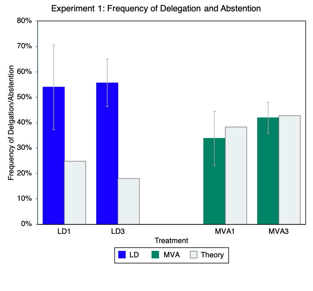
Figure 2: Aggregate frequency of delegation and abstention. Confidence intervals are calculated from standard errors clustered at the session level.

The result is unambiguous: delegation rates in the experiment are between two and three times what theory predicts for the equilibrium that improves over MV. Abstention rates on the other hand are comparable to the predictions. With such high propensity to delegate, the conclusion is robust to all plausible ways of cutting the data: disaggregating by session, considering only the 10 final rounds, clustering standard errors at the individual level.

Regressions on individual behavior that control for signal quality and for round and treatment order effects lead to the same conclusion. Tables 4 and 5 report linear probability and probit regressions, with Table 4 referring to LD1 and MVA1 ($N=5$); Table 5 to LD3 and MVA3 ($N=15$). In both tables, the excluded case is MVA played as first treatment in MVA-only sessions. Standard errors are clustered at the session level. As expected, the propensity to abstain or delegate is affected negatively by higher precision of the signal, similarly across the two group sizes. Order effects matter but, controlling for order and for signals precision, delegation remains higher than abstention: the coefficient of the LD dummy is positive in both tables. Recall that the theoretical prediction is in the opposite direction: abstention is predicted to be more frequent than delegation.

Experiment 1: Frequency of Delegation or Abstention. N=5.
	(1)	(2)
	Linear Probability	Probit
LD	0.328***	0.938***
	(0.073)	(0.274)
	[0.006]	[0.001]
Signal Precision	-0.777***	-2.624***
	(0.080)	(0.307)
	[0.000]	[0.000]
Second	0.154***	0.534***
	(0.010)	(0.026)
	[0.000]	[0.000]
Second * Mixed	-0.129***	-0.451***
	(0.002)	(0.025)
	[0.000]	[0.000]
LD * Second	-0.090	-0.332**
	(0.050)	(0.160)
	[0.134]	[0.038]
LD * Second * Mixed	-0.025***	-0.033
	(0.006)	(0.022)
	[0.008]	[0.140]
Constant	0.675***	0.582***
	(0.0475)	(0.128)
	[0.000]	[0.000]
Observations	1,920	1,920
R-squared	0.309
*** p<0.01, ** p<0.05, * p<0.1

Table 4: Determinants of delegation and abstention; N=5. Standard errors in parentheses, clustered at the session level.

Experiment 1: Frequency of Delegation or Abstention. N=15.
	(1)	(2)
	Linear Probability	Probit
LD	0.208**	0.677***
	(0.071)	(0.249)
	[0.022]	[0.007]
Signal Precision	-0.861***	-2.691***
	(0.047)	(0.208)
	[0.000]	[0.000]
Second	-0.096**	-0.341***
	(0.035)	(0.126)
	[0.029]	[0.007]
Second * Mixed	0.078***	0.295***
	(0.006)	(0.030)
	[0.000]	[0.000]
LD * Second	0.037	0.125
	(0.037)	(0.132)
	[0.349]	[0.343]
LD * Second * Mixed	-0.166**	-0.577***
	(0.055)	(0.183)
	[0.019]	[0.002]
Constant	0.832***	0.992***
	(0.069)	(0.237)
	[0.000]	[0.000]
Observations	2,880	2,880
R-squared	0.309
*** p<0.01, ** p<0.05, * p<0.1

Table 5: Determinants of delegation and abstention; N=15. Standard errors in parentheses, clustered at the session level. P-values in brackets. Delegation/abstention is measured as a binary 0-1 subject decision. “Second” indicates that the treatment appeared second in the session. “Mixed” indicates that both an LD treatment and an MVA treatment appeared in the session. Controls for round, the interaction of LD and round, and the interaction of LD and signal precision are included.

Participants’ choices appear coherent, if not optimal. Delegation and abstention decisions are not only negatively correlated to signals precision, as the regressions show; we find that they are also monotonic in signal precisions (if non-expert $i$ votes at precision $q(i)$, then $i$ votes at all $q^{\prime}(i)>q(i)$). We report histograms of monotonicity violations for all four treatments in the Appendix. There is weak evidence of fewer violations under MVA, but the two treatments are effectively comparable. Just below 60% of subjects have no violations at all under LD; just above 60% under MVA, and the results are invariant to the size of the group. In all cases, it is possible to generate perfect monotonicity for at least 80 percent of participants by changing at most 2 of their non-expert choices.

We use monotonicity to estimate individual precision thresholds for delegation and abstention–the thresholds below which each participant delegates or abstains. Figure 3 reports, for each participant, the mean of the range of thresholds that are consistent with minimal monotonicity violations; the size of the dots is proportional to the number of participants at that threshold. The dark blue (for LD) and dark green (for MVA) diamonds correspond to the average empirical thresholds, and the respective light ones to the theory. The figure confirms the over-delegation that characterizes LD, while again average values for abstention are close to the theoretical predictions. The dispersion in estimated thresholds is typical of similar experiments (for example, Levine and Palfrey, 2007; Morton and Tyran, 2011), but is in clear tension with the focus on symmetric equilibria.

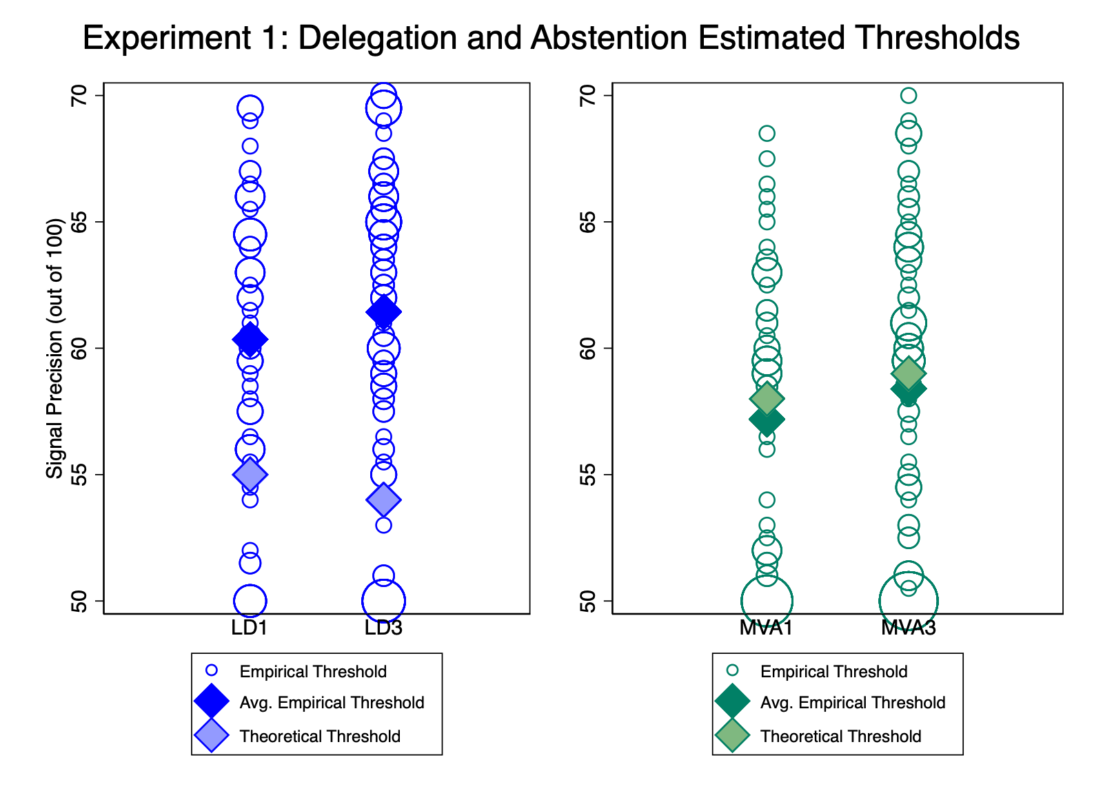
Figure 3: Individual delegation and abstention thresholds.

The observation that thresholds tend to be higher for delegation rather than abstention is confirmed in Figure 4, where we plot the cumulative distribution functions of the estimated thresholds.

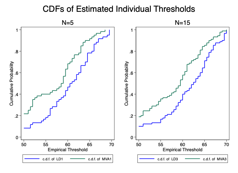
Figure 4: Individual delegation and abstention thresholds. CDFs.

For both group sizes, the LD distribution, in blue, first order stochastically dominates the MVA distribution, in green: at any precision, including at the lower boundary of the support, the fraction of subjects estimated to delegate is above the corresponding fraction of abstainers (the fraction of subjects whose estimated threshold is below the threshold, and thus are voting at that precision, is lower). Two-sample Kolmogorov-Smirnov tests adjusted for discreteness confirm the visual impression: for both group sizes, the probability that the two samples of thresholds, for LD and for MVA, are drawn from the same distribution is very low ($p=0.034$ for $N=5$, and $p=0.0047$ for $N=15$). On the other hand, for given voting system, allowing delegation or abstention, the data do not show substantive differences between the two group sizes.

6.2 Frequency of correct choice

Beyond regularities of delegation and abstention, the real variable of interest is the frequency with which the voting system leads to the correct choice. We begin by reporting the data. Because we are studying variations of majority voting, a large share of outcomes under both LD and MVA correspond to MV. Testing the relative performance of the voting systems requires conditioning on reaching different outcomes, and we will move to that after describing the data.

Figure 5 reports the experimental data and compares them to the theoretical interior equilibrium and to MV.

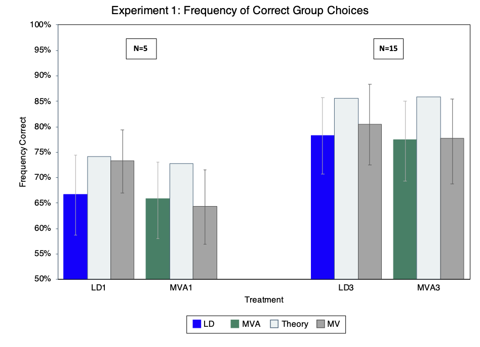
Figure 5: Frequency of correct outcomes. For subjects who delegated or abstained, MV data allow voting against signal with probability equal to the frequency observed in the treatment. Confidence intervals are calculated from bootstrapping, using 100,000 simulated data sets and allowing for within-subject correlation.

We report results grouped by $N$. The vertical axis is the frequency of correct outcomes over the full data set for the corresponding treatment. The figure holds three main lessons. First, for both group sizes, LD and MVA yield very similar frequencies of correct decisions. Second, for both group sizes, both systems fall short of their possible best performance. Third, MVA outcomes are closely comparable to MV for both group sizes, but LD outcomes fall short of MV, especially for small groups.

Two main deviations could be responsible for the systems’ underperformance relative to the theory. The first is the erroneous choice of delegation/abstention thresholds. Figures 2 and 3 support this interpretation for LD, with its consistent over-delegation, but not for MVA. The second is random voting in the form of voting against signal. As we show in the Appendix, the frequency of voting against signal correlates negatively and significantly with signal precision. Thus experts vote against signal more rarely than non-experts. Both because experts cast multiple votes under LD, and because subjects choose to vote at lower precision under MVA, the share of votes cast against signal is lower in the LD treatments (at about 6%) than in the MVA ones (at about 10%), with little difference across group sizes. MVA suffers from more random voting. Both systems thus fail to realize their potential gains over MV, but for different reasons.

The comparison to MV shows that the penalty is higher for LD. The better performance of MV in the LD samples reflects the random superiority of the signal draws in those samples: although signal realizations were drawn from the same probability distribution, the frequency of correct signals was higher in the LD treatments. Thus, although LD and MVA have similar shares of correct decision in our data, LD treatments could have performed better, given the superiority of the realized signals.

6.2.1 Comparing LD and MVA to MV

Evaluating the significance of the disparities observed between LD or MVA on one side, and MV on the other is not immediate. One difficulty is the complexity of the correlation structure, but the fundamental difficulty is simpler: as mentioned above, outcomes coincide in a large majority of cases. Restricting the data sample to those elections in which outcomes differ leaves us with little information. To overcome this difficulty, we use bootstrapping methods to simulate a large number of elections in a population for which our data are representative. By simulating many elections, conditioning on different outcomes becomes feasible.

The procedure we implement allows for correlation across an individual’s multiple decisions, and uses randomization to generate the correct balance of experts and non-experts. For each voting system and group size, we generate outcomes by drawing subjects, with replacement, each with their full set of 20-round decisions, and matching them randomly into groups. We then study the outcomes corresponding to 100,000 replications of the experiment for each treatment, using the population of subjects for that voting system and group size. We describe the procedure in more detail in the online Appendix. Figure 6 shows the distributions of the differential frequency of correct decisions between the voting systems we are studying and MV, for each group size, conditioning on the decisions being different. Consider for example LD1. For each of the 100,000 simulations, we focus on the subset of elections $D_{LD1}$ such that LD1 and MV reach a different outcome. Call $\gamma_{LD1}(D_{LD1})$ $(\gamma_{MV}(D_{LD1}))$ the frequency with which LD1 (MV) is correct over subset $D_{LD1}$, a variable that ranges from 0 to 1. We are interested in $\gamma_{LD1}(D_{LD1})-\gamma_{MV}(D_{LD1})$, where, by construction, $\gamma_{MV}(D_{LD1})=1-\gamma_{LD1}(D_{LD1})$. Hence $\gamma_{LD1}(D_{LD1})-\gamma_{MV}(D_{LD1})=2\gamma_{LD1}(D_{LD1})-1$. Our measure then ranges from 1—when, conditional on disagreement, LD1 always reaches the correct outcome, and MV the incorrect outcome—to $-1$, when the opposite holds; a value of zero indicates that the two rules are correct with equal frequency, conditioning on disagreement. The first panel of Figure 6 plots, in blue, the distribution of such variable over the 100,000 replications. The equivalent distribution for MVA is plotted in the same panel in green. The second panel reports the results for groups of size 15.

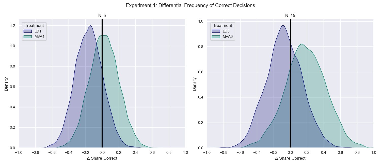
Figure 6: Differential frequency of correct decisions, relative to MV, conditional on different outcomes. Distributions over 100,000 bootstrap replications.

For both group sizes, the blue distribution is shifted to the left, relative to the zero point indicated by the vertical black line: when LD and MV differ, the correct decision is more likely to be the one reached by MV. The asymmetry is more pronounced for $N=5$, where the blue mass to the left of zero – the probability that MV is superior to LD1, conditional on disagreement—is 85%, versus 67% for LD3. MVA on the other hand, when disagreeing with MV, is more likely to be right than wrong: only barely when $N=5$ and the probability that MV is superior to MVA1 is just below 50% (48%), but more substantially when $N=15$ and the probability that MV is correct, conditional on disagreement with MVA3, falls to 26%. The distributions are also informative of the quantitative gap in the probability of being correct, relative to MV. In the panel on the left, for example, the mode of the blue distribution at -16% tells us that over the 100,000 replications, conditional on disagreement, the highest probability mass is around a frequency of correct decisions of about 42% for LD1, versus 58% for MV.

In our first experiment then, LD falls short of the hopes if its supporters, even in a streamlined environment where experts are correctly identified. Like delegation, abstention allows voters with weak information not to influence the final choice, but is simpler and performs better. In our data, its efficiency is either comparable or somewhat superior to universal majority voting, contrary to what we see for delegation.

But do these results reflect some core feature of the systems we are studying, or are they artifacts of the lab? We analyze this question in our second experiment.

7 Experiment 2: The Random Dot Kinematogram

As discussed in the Introduction, the goal of our second experiment is to evaluate whether the deviations from optimal behavior we see in the lab may stem from the over-mathematization of the environment. There are three possible concerns. First, the precise numerical description of the signals’ precisions makes the difference between one’s own precision and the expert’s very salient. At the same type, and this is the second concern, such precision can also induce suboptimal behavior among subjects who choose to vote: participants could plausibly think that a signal precise with probability not much above 50% should be disobeyed about half the time. Finally, our formulation could be biasing the analysis in favor of MV by positing that all signals are correct with probability larger than 50%, an assumption likely to be correct on average but occasionally violated. It is not clear why a detailed mathematical frame should affect the relative performance of delegation and abstention, but it is quite possible that the frame’s high precision may distort behavior. With this in mind, we chose for the second experiment a perceptual task—the Random Dot Kinematogram (RDK)—where individual signals correspond to the accuracy of individual perceptions, and neither own nor others’ accuracies are described or known in precise probabilistic terms. Because the task may be unfamiliar, we describe it in some detail.

We ran the experiment on Amazon Mechanical Turk (with prescreening of subjects by CloudResearch) with three electorate sizes: $N=5$ and $N=15$, as in Experiment 1, but also $N=125$, i.e. with a larger size than we could run in the lab or conveniently on Zoom. In our implementation, 300 moving dots appear in each subject’s screen for 1 second; a small fraction of them (dependent on treatment) moves in a coherent direction, either Left or Right, with equal ex ante probability; the rest move randomly. After 1 second, the image disappears and each participant reports whether the perceived coherent direction was Left or Right. We divide the experiment into two parts, each preceded by a few practice tasks, but with the first part effectively playing the role of extended training. Both parts are divided into six blocs, with each bloc consisting of 20 tasks of equal coherence. We report in the online Appendix the precise parameters we used for the task (the size and color of the dots, the movements per frame, the random process for the dots moving randomly, etc.), but it should be clear that our experiment does not aim at measuring perception per se—for example, we cannot control the ambient light, screen size, or contrast of the monitors our subjects use. Our focus remains on collective decision-making.

In Part 1, subjects are rewarded on the basis of their individual accuracy. Coherence—the fraction of dots that move in the same direction—ranges from 20% in bloc 1 (one fifth of the 300 dots move synchronously) to 10% in bloc 2, 8% in bloc 3, 6% in bloc 4, and finally the same coherence used in Part 2, smaller and dependent on $N$, for the final two blocs. At the end of Part 1, each subject is informed of her fraction of correct answers in each bloc. In part 2, each task has both an individual component (“Choose the coherent direction”), and a subsequent group decision with the possibility of delegation (under LD), or abstention (under MVA). (“You said Left. Do you want to Vote or to Delegate (Abstain)?”). When delegation is chosen, the vote is assigned randomly to an “expert,” that is, one of the participants whose accuracy is in the top 20% of the group over the last 2 blocs (40 tasks); experts are not allowed to delegate (under LD) or to abstain (under MVA). Thus in line with Experiment 1, groups of 5 have 1 expert, and groups of 15 have 3; the group of 125 has 25 experts, and, following our standard notation, we denote the two treatments on the larger group by LD25 and MVA25. The group decision corresponds to the majority of votes cast, and individuals are rewarded both for their individual accuracy and for the accuracy of the group. As in Part 1, feedback about average individual accuracy in each bloc is provided at the end of Part 2. In Part 2, coherence is kept constant across all blocs. We chose its value according to two main criteria: the task should not be so difficult that subjects are discouraged and act randomly, and should not be so easy that MV accuracy, especially in the large group, leaves effectively no room for possible improvement. Based on the results of two preliminary pilots, we fixed coherence in Part 2 at 5% for electorates of sizes 5 and 15, and at 3% for the electorate of size 125. The task is objectively hard, as the reader can verify at the following link: https://blogs.cuit.columbia.edu/ac186/files/2022/05/rdk-video.gif

The experiment used the RDK plugin in jsPsych (Rajananda et al., 2018) and was hosted on cognition.run. For each of LD and MVA, we recruited 60 subjects divided into 12 groups for the $N=5$ treatment and 90 subjects divided into 6 groups for $N=15$ (thus replicating the corresponding number of subjects and groups in Experiment 1), and an additional 125 subjects for the largest group. There were then 275 subjects for each voting system, or 550 in total. The group size and the relevant number of experts were always made public. The experiment lasted about 20 minutes. Subjects earned $1 for participation and a bonus proportional to the number of correct responses, for a total average compensation of $4.92, or just below $15 an hour.

8 Experiment 2: Results

8.1 Accuracy

We define an individual’s accuracy as the fraction of correct responses. Figure 7 reports the distributions of accuracy in Part 2 calculated over each of the 6 blocs for each subject, that is, over 20 tasks. The two panels correspond to the two levels of coherence used in the experiment (0.05 on the left; 0.03 on the right).

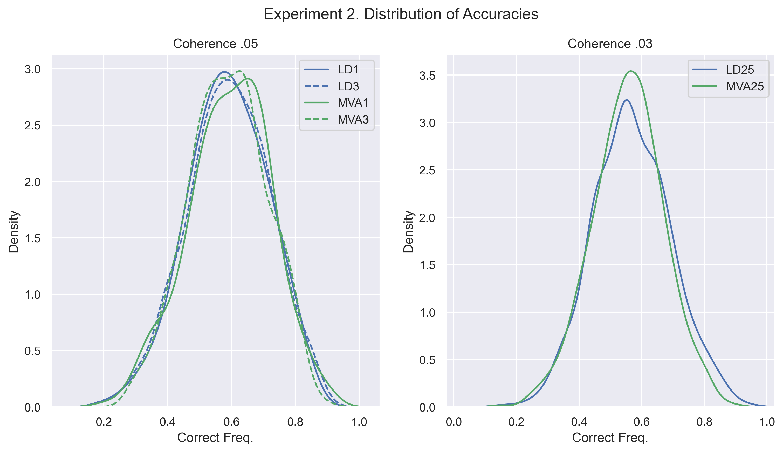
Figure 7: Accuracies per bloc per subject. Distributions. A bloc consists of 20 tasks.

For given coherence, the distributions are very similar across treatments. In all cases, the spread in the distribution of accuracies is large, ranging from about 25% all the way to 95%. Mean accuracy over all participants is 59% in treatments with 0.05 coherence, and 56% in treatments with 0.03 coherence. Experts’ accuracy is higher than non-experts’: average accuracy per bloc is 63% for experts (v/s 58% for non-experts) in treatments with 0.05 coherence, and 59% (v/s 55.5%) in treatments with 0.03 coherence.

The frequency of blocs with accuracy below 50% is non-negligible (18% for coherence of 0.05, just above 23% for coherence of 0.03) and, surprisingly, persists when we aggregate over a larger number of tasks. Averaging at the subject level over all 120 tasks, 9% of subjects have accuracy below randomness with coherence 0.05, and 12% with coherence 0.03. If we want to study voting and information aggregation when information may be faulty, perceptual tasks can provide a very useful tool.

8.2 Frequency of delegation and abstention

Absent information about the distributions of subjects’ beliefs, we do not have a theoretical reference point for the extent of delegation and abstention we see in the data. We can however compare the two, under the plausible assumption, supported by Figure 7, that accuracies and beliefs about accuracies are comparable across the LD and MVA samples. Figure 8 plots the frequencies of delegation and abstention for each group size, calculated over non-experts only for possible comparison to Experiment 1. The 95% confidence intervals are calculated from standard errors clustered at the individual level.

Figure 8: Aggregate frequency of delegation and abstention (non-experts). 95% confidence intervals calculated from standard errors clustered at the individual level.

In Experiment 2, delegation remains much more common than abstention, for all group sizes. In groups of 5, where the disparity is largest, delegation is more than twice as frequent; in groups of 15, where we see the least disparity, delegation is still 60% more common. The decline in coherence, from $N=5$ or $15$ to $N=125$, has small effects on the data. Unexpectedly, considering the rather radical change in experimental design, Figure 8 is very similar to Figure 2, for the group sizes for which we have data from both experiments.

The higher frequency of delegation is confirmed in the regressions reported in Tables 6 and 7. The unit of analysis is the bloc at the individual subject level (hence 6 blocs per subject), with data grouped by coherence level. The regressions reported below confirm the results of the figure: in all treatments, delegation is significantly more frequent than abstention. In Experiment 2, accuracy is at best a very weak predictor of participation in voting, never significant at conventional levels and with the wrong sign in the probit estimation, confirming the high uncertainty in subjects’ evaluation of their own accuracy. The probit regressions detect a decline in abstention as blocs proceed, which is consistent with increased familiarity with the task.

Experiment 2: Frequency of Delegation or Abstention. N=5 and N=15.
	(1)	(2)	(3)	(4)
	Linear Probability	Linear Probability	Probit	Probit
Accuracy	-0.122	-0.122	0.356	0.354
	(0.084)	(0.084)	(0.309)	(0.308)
	[0.146]	[0.146]	[0.249]	[0.251]
LD	0.226***	0.226***	0.547***	0.548***
	(0.038)	(0.038)	(0.139)	(0.140)
	[0.000]	[0.000]	[0.000]	[0.000]
N=15	0.005	0.004	0.051	0.05
	(0.038)	(0.038)	(0.139)	(0.140)
	[0.907]	[0.908]	[0.717]	[0.719]
Keys: [E][Y]		-0.009		-0.04
		(0.038)		(0.139)
		[0.816]		[0.772]
Bloc		0.001		-0.256***
		(0.012)		(0.065)
		[0.965]		[0.000]
Constant	0.339***	0.343***	0.163	0.313
	(0.063)	(0.066)	(0.222)	(0.234)
	[0.000]	[0.000]	[0.463]	[0.181]
Observations	1,800	1,800	1,800	1,800
R-squared	0.100	0.100
*** p<0.01, ** p<0.05, * p<0.1

Table 6: Frequency of delegation/abstention; $N=5$ and $N=15$. Standard errors are clustered at the individual level.

Experiment 2: Frequency of Delegation or Abstention. N=125.
	(1)	(2)	(3)	(4)
	Linear Probability	Linear Probability	Probit	Probit
Accuracy	0.000	0.004	0.479	0.455
	(0.101)	(0.102)	(0.357)	(0.359)
	[0.998]	[0.970]	[0.180]	[0.205]
LD	0.224***	0.223***	0.661***	0.663***
	(0.042)	(0.042)	(0.164)	(0.164)
	[0.000]	[0.000]	[0.000]	[0.000]
Keys: [E][Y]		0.029		-0.043
		(0.041)		(0.161)
		[0.484]		[0.790]
Bloc		0.002		-0.0363**
		(0.003)		(0.015)
		[0.459]		[0.014]
Constant	0.316***	0.282***	0.313	0.694**
	(0.062)	(0.072)	(0.225)	(0.288)
	[0.000]	[0.000]	[0.163]	[0.016]
Observations	1,500	1,500	1,500	1,500
R-squared	0.095	0.097
*** p<0.01, ** p<0.05, * p<0.1

Table 7: Frequency of delegation/abstention; $N=125$. Standard errors are clustered at the individual level. P-values in brackets. Delegation/abstention is measured as the share of rounds in a given bloc in which a subject chose to delegate/abstain (with a range from 0 to 1). Accuracy is the share of rounds in the bloc that subject answered correctly. Subjects randomly use either keys [V] and [N] or [E] and [Y] to decide whether to vote; a dummy for being assigned [E][Y] is included. The values for bloc have been scaled to be between 0 and 1; the coefficient for “bloc” thus indicates the effect of going from the first to last bloc.

8.3 Frequency of correct outcomes

How well did the three voting systems do in Experiment 2? Figure 9 reports the frequency of correct group decisions, aggregated over all groups and tasks for given treatment. As in the case of Figure 5, a large fraction of outcomes are identical.

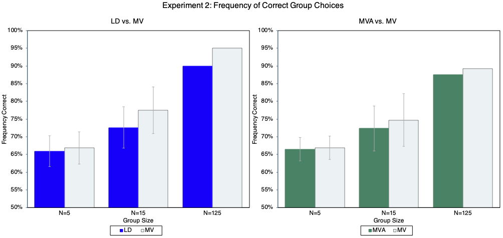
Figure 9: Frequency of correct outcomes. 95% confidence intervals are calculated from standard errors clustered at the group level.

As expected, for all three systems, the fraction of correct decisions increases with the size of the group, ranging from about 65% at $N=5$ to 90-95% at $N=125$. In this pure common interest environment, the aggregation of independent signals remains very powerful, even in the presence of weak accuracies. In line with this logic, and with Condorcet, universal voting consistently achieves the best results. Here too, for the group sizes that are common to both experiments, the numbers are surprisingly similar to the numbers in Figure 5. Relative to MV, MVA performs better than LD, but the result could simply reflect the lower propensity to abstain. Because abstention is less common, the fraction of decisions in which MVA and MV disagree is about half the fraction under LD (between 8 and 12% across the different treatments under MVA, v/s 12 to 24% under LD). And if MVA and MV agree more, their performance overall is more similar. To achieve better estimates of the differences across the three voting systems, we again bootstrap the data and replicate the group decisions a large number of times, generating a large sample of decisions over which the voting results differ, as we did with the data from Experiment 1.

Figure 10 reports the results of 100,000 simulations, with three panels corresponding, in order, to $N=5$, $N=15$, and the single large group at $N=125$. As in Figure 6, we plot the distributions of the differential frequency of correct decisions under LD (in blue) or MVA (in green), relative to MV. Recall that, if the distribution is skewed to the left of the vertical line at zero, then conditional on disagreement, the correct decision is more likely to be the one reached by MV; and vice-versa if the distribution is skewed to the right.

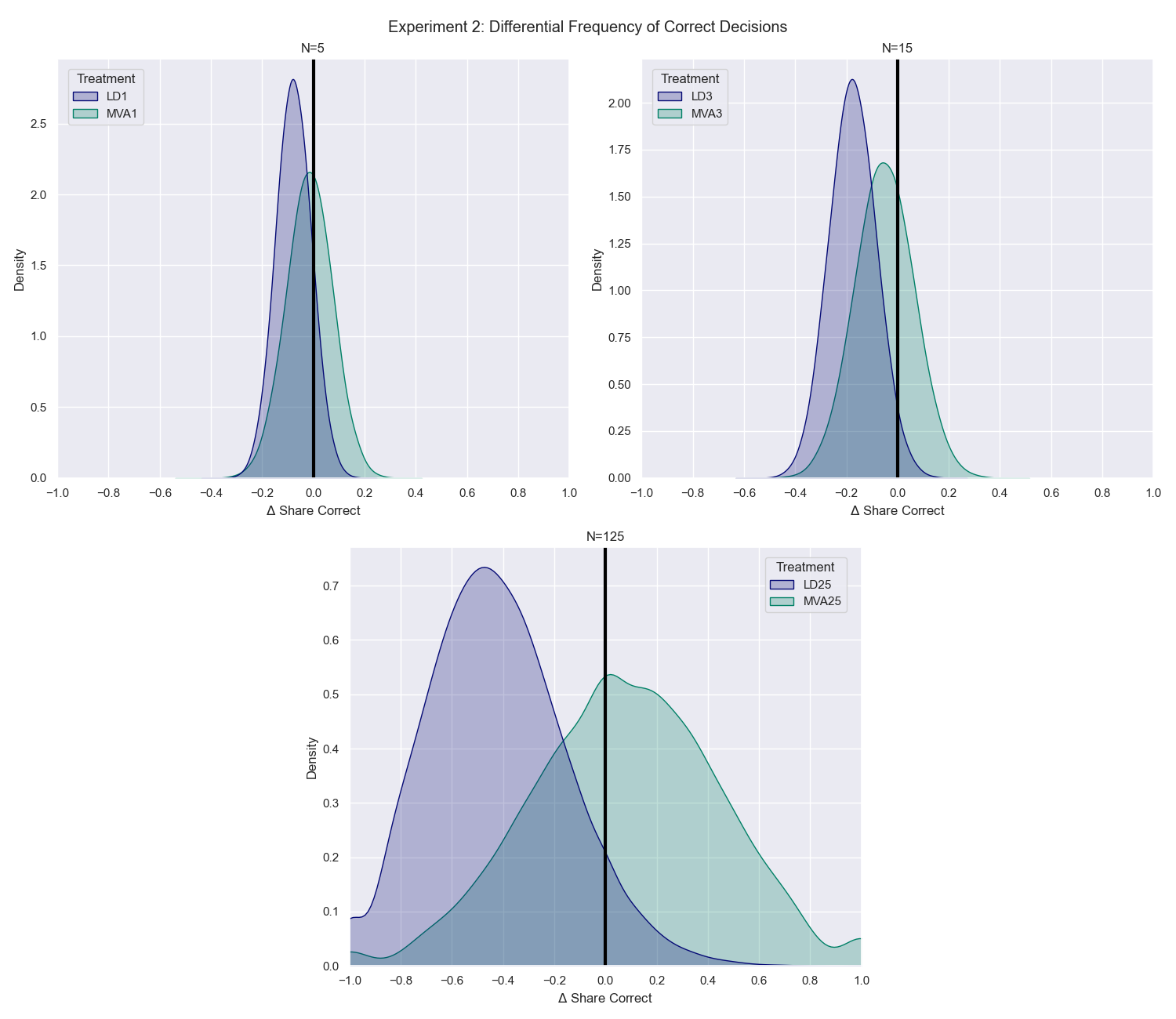
Figure 10: Differential frequency of correct decisions, relative to MV, conditional on different outcomes. Distributions over 100,000 bootstrap replications.

In all three panels, the blue mass is shifted to the left. Conditional on disagreement, the share of simulated experiments in which MV is more likely than LD to yield the correct outcome is 87% for LD1, 97% for LD3, and 95% for LD25. MVA (green in the figure) fares better: the corresponding numbers are 58% for MVA1, 69% for MVA3, and 48% for MVA25, when MVA is just barely more likely to be correct than MV, conditional on disagreement. As in Figure 6, the shapes of the distributions tell us the frequencies with which the two systems are correct, relative to MV. The proximity to zero indicates that even if the voting rule performs less well than MV, the difference need not be large. When $N=5$ for example, the mode of the blue distribution at -0.08 says that over the 100,000 simulations the most likely result is a frequency of correct decision of 46% for LD1 versus 54% for MV.

In perceptual research, the focus is the immediate, apparently unconscious reaction to the stimulus, and the experimental design minimizes interference with such a process. With this in mind, we chose not to ask participants for their beliefs within each task. We did, however, add two summary questions at the end of the experiment. We asked: “On average, what percentage of trials in the second part do you think you got right?”, and “On average, what percentage of trials in the second part do you think the experts got right?” With only these two questions, barely incentivized, our information on beliefs can only be very noisy. We report our findings in more detail in the online Appendix, but, without making too much of them, they can be summarized briefly. In all treatments, beliefs about own accuracy track actual accuracy surprisingly well: for treatments with 0.05 coherence, average believed accuracy is 58% (v/s 59% for average realized accuracy); with coherence 0.03, average believed accuracy is 55% (v/s 56% for average realized accuracy). Beliefs about experts’ accuracy are inflated by about 15% at both coherence levels (71% v/s 63% at 0.05 coherence, and 70% v/s 59% at 0.03 coherence). We saw in Tables 6 and 7 that accuracy is a very weak predictor of choosing to vote. Beliefs about own and the experts’ accuracy are instead strong predictors of the decision to vote. Beliefs, however, cannot explain the difference in the frequency of delegation and abstention.

9 Conclusions

Liquid Democracy is a computer-mediated voting system where all decisions are subject to popular referendum but voters can delegate their votes. The option of delegation to better informed experts seems intuitively valuable, and indeed, theory shows that if experts are correctly identified, delegation improves the chances of reaching the correct decision. However, delegation must be used sparingly because, by reducing the number of independent voices, it also reduces the aggregate amount of information expressed by the electorate. This paper reports the results of two very different experiments that measure participants’ propensity to delegate their vote and compare the decisions of the group when delegation is possible, when abstention is possible, and under universal majority voting. In line with Condorcet’s message, we find that in both experiments universal majority voting leads to the highest frequency of correct outcomes, even in small groups; abstention is closely comparable, but delegation is inferior to both, even in our simplified world where experts are indeed better informed. The reason is that the option of delegation is chosen too frequently—two to three times more frequently than optimal in the experiment where we have a precise theoretical prediction.

The environment we study abstracts from information costs. Allowing for such costs would make delegation more valuable because voters for whom the acquisition of information is more difficult can defer to others. Introducing information costs explicitly may be a good direction for future work. Note however that the saving on information costs is also possible through abstention. And in our experiments at least, such alternative is used less frequently and with better results.

On informational grounds alone, the experiments we ran do not support the arguments in favor of Liquid Democracy. The next step is to run such experiments again under controlled conditions, but in the field. If the results are confirmed, other arguments invoked for Liquid Democracy should then be given weight and studied—the advantages, and weaknesses, of direct democracy; the heightened sense of responsibility of an empowered electorate in this more participatory form of democracy.

The second contribution of this paper is methodological. We match a canonical, fully controlled lab experiment on voting with a perceptual experiment where information is ambiguous: participants do not know the probabilities with which either their own or the experts’ information is correct. We use such a design because there are plausible concerns that the precise mathematical framing of the canonical experiment may affect the results. In addition, the ambiguity of the information in the perceptual experiment seems closer to realistic conditions of voting for political decisions. In fact, we find that the results of the first experiment replicate closely in the second. The robustness of the conclusions is a central contribution of our study. Beyond the specific results, perceptual experiments are a very useful tool for the study of group decision-making when we want to allow information to be ambiguous, especially in combination with the more controlled environment of traditional lab experiments on voting. Social psychologists have been studying them for decades; it is time economists interested in social choice added them to their tool box as well.

Appendix A Appendix

A.1 Theoretical results

Theorem.

Suppose $\pi=Pr(\omega_{1})=1/2$. Then for any $F$ and for any $N$ and $K$ odd and finite, there exists an equilibrium with delegation that strictly improves over MV.

The proof proceeds in four steps. We begin with Lemma 1:

Lemma 1.

Consider a profile of strategies $\Sigma=\{\Sigma_{ne},\Sigma_{e}\}$ symmetric for voters of each class, and such that votes are cast according to signal and delegation decisions are symmetric with respect to signals’ realization. There exists a profile $\Sigma^{*}=\{\Sigma_{ne}^{*},\Sigma_{e}^{*}\}\in\{\Sigma_{ne},\Sigma_{e}\}$ such that $EU(\Sigma^{*})\geq EU(\Sigma)$ for all $\Sigma\neq\Sigma^{*}.$

Proof.

If all votes cast are cast according to signal, strategic choices are limited to delegation. Because we are focusing on delegation strategies that are symmetric with respect to signals’ realizations, such strategies depend on signals’ precisions only. Consider first non-expert $i$. Keeping in mind that all $q_{i}$’s are independent draws from $F(q)$, expected utility conditional on delegation—$EUD_{i}^{(e)}$ for delegation to an expert, or $EUD_{i}^{(ne)}$ for delegation to a non-expert—does not depend on $q_{i}$ (because $i$ would not be voting). On the other hand, $i$’s expected utility when not delegating, $EUND$, must be weakly increasing in $q_{i}$ (because the probability of reaching the correct outcome must be weakly increasing in $q_{i}$), and strictly increasing if $i$’s probability of being pivotal is positive. It follows that in any equilibrium there must exist a $\widetilde{q}\in$$[\underline{q},\overline{q}]$ such that individual $i$ votes (according to signal) if $q_{i}\geq\widetilde{q}$, and delegates otherwise. If $q_{i}<\widetilde{q}$, non-expert $i$ will delegate and may delegate to either an expert (with probability $\delta^{(e)}$) or to a non-expert (with probability $\delta^{(ne)})$. These probabilities may correspond to realizations of $q_{i}$ in different subintervals, but the precise characterization of such sub-intervals is irrelevant because upon delegation $q_{i}$ has no effect on expected utility. Hence symmetric non-expert $i$’s delegation strategies are summarized by a set of three numbers $\Sigma_{ne}=\{\delta^{(e)},\delta^{(ne)},\widetilde{q}\}$, with $\delta^{(e)}+\delta^{(ne)}=F(\widetilde{q})\in[0,1]$ and $\widetilde{q}\in$$[\underline{q},\overline{q}]$. In the case of expert individuals, precision is fixed at $p$. Hence, denoting by $\xi^{(e)}(\xi^{(ne)})$ an expert’s probability of delegating to another expert (non-expert), strategies are given by $\Sigma_{e}=\{\xi^{(e)},\xi^{(ne)}\}$, with $\xi^{(e)}+\xi^{(ne)}\in[0,1]$. Although the set of strategies $\Sigma$ is infinite, it is compact. Because $EU$ is a continuous function of $\Sigma$, we can then apply Weierstrass’s Theorem, and the conclusion follows: there exists a profile $\Sigma^{*}=\{\Sigma_{ne}^{*},\Sigma_{e}^{*}\}\in\{\Sigma_{ne},\Sigma_{e}\}$ such that $EU(\Sigma^{*})\geq EU(\Sigma)$ for all $\Sigma\neq\Sigma^{*}.$ ∎

Lemma 2.

The profile of strategies $\Sigma^{*}$ is an equilibrium.

Proof.

The result is established in two steps, both derived from McLennan (1998). First, restrict attention to profiles of semi-symmetric strategies with sincere voting and symmetric delegation with respect to signals’ realization. Within such profiles, $\Sigma^{*}$ is maximal (i.e. $\Sigma^{*}=argmax_{\Sigma}EU(\Sigma)$) by construction. But in this pure common interest game, it then follows that $\Sigma^{*}$ must be an equilibrium (McLennan, Theorem 1). Second, the environment is fully symmetric for each class of individuals, experts and non-experts, and at any such type-symmetric strategy profile, with sincere voting and symmetric delegation, no voter wants to deviate to asymmetric delegation or an insincere voting strategy. A priori the two states are equally likely, and the precision of the signals does not depend on the state. All voters have identical preferences and are endowed with a single vote. All experts have equal precision and equal probability of receiving any delegated vote, and thus, for any delegation strategy by non-experts, each expert’s vote has equal expected weight on the final decision. Non-experts will have heterogeneous realized precisions, and the equilibrium action will depend on individual precision, but each precision $q_{i}$ is an independent draw from the same distribution $F$. Hence any permutation of realized precisions to different non-expert voters is assigned equal probability, and each voter holds equal beliefs about the others’ precisions. For each type of voter, these symmetry conditions satisfy the requirements of McLennan’s Theorem 2: if $\Sigma^{*}$ is maximal with respect to semi-symmetric strategies with sincere voting and symmetric delegation, then it is an equilibrium over all profiles of strategies. Note that asymmetric equilibria may exist, and be superior to $\Sigma^{*}.$ ∎

Lemma 3.

Sincere majority voting is not an equilibrium.

Proof.

Sincere majority voting is feasible within the set of strategies $\Sigma$ (semi-symmetric strategies with delegation symmetric across signals and sincere voting). It corresponds to $\widetilde{q}=\underline{q}$ (and thus $\delta^{(e)}=\delta^{(ne)}=0)$, and $\xi^{(e)}=\xi^{(ne)}=0$. Can such set of strategies be an equilibrium? If the answer is negative, then we know, by the previous results, that there must exist an equilibrium of the LD voting game that strictly dominates MV and involves delegation.

Consider the perspective of non-expert voter $i$, with $q_{i}$ in the neighborhood of $\underline{q}$. Suppose no-one else delegates. We show in what follows that $i$’s best response is to delegate his vote. Note first that if no-one delegates, all non-$i$ voters cast a single vote and have equal weight on the group decision. Hence if $i$ delegates, it is optimal to delegate the vote to an expert, with precision $p\geq q_{j}$ for all $j$.

We need to calculate $i$’s interim expected utility from non-delegating ($EUND(q_{i}))$ or delegating ($EUD)$. The expressions are somewhat cumbersome but conceptually straightforward. We find:

$$EUND(q_{i}),=\sum_{c_{n}=0}^{M-1}\binom{M-1}{c_{n}}\mu^{c_{n}}(1-\mu)^{M-1-c_{n}}\times\\ \times\left[\sum_{c_{e}=0}^{K}\binom{K}{c_{e}}p{}^{c_{e}}(1-p)^{K-c_{e}}\left(q_{i}I_{c_{n}+c_{e}+1>\frac{(M+K)}{2}}+(1-q_{i})I_{c_{n}+c_{e}>\frac{(M+K)}{2}}\right)\right]$$

$$EUD=\sum_{c_{n}=0}^{M-1}\binom{M-1}{c_{n}}\mu{}^{c_{n}}(1-\mu)^{M-1-c_{n}}\times\\ \times\left[\sum_{c_{e}=0}^{K}\binom{K}{c_{e}}p{}^{c_{e}}(1-p)^{K-c_{e}}\left(\left(\frac{c_{e}}{K}\right)I_{c_{n}+c_{e}+1>\frac{(M+K)}{2}}+\left(\frac{K-c_{e}}{K}\right)I_{c_{n}+c_{e}>\frac{(M+K)}{2}}\right)\right],$$

where $M$ is the number of non-experts, $c_{n}$($c_{e}$) indexes the number of non-experts other than $i$ (experts) whose signals are correct, $\mu$ is the expected precision of non-experts who choose to vote, and thus in this conjectured scenario, $\mu=\int_{\underline{q}}^{\overline{q}}qdF(q)$, and $I_{C}$ is an indicator function that takes value $1$ if condition $C$ is satisfied and $0$ otherwise. For each realized $c_{n}$ and $c_{e}$, $i$’s expected utility always equals 1 if $(c_{n}+c_{e})>(M+K)/2$, i.e. if the other voters with correct signals constitute a majority of the electorate. For $i$, the choice to delegate or not matters when $(c_{n}+c_{e})$ falls short of the majority by one vote. In such a case, $EUND(q_{i})$ equals 1 if $i$’s own signal is correct (with probability $q_{i}$) and zero otherwise; $EUD$ equals 1 if $i$’s vote is delegated to an expert with a correct signal (with probability $c_{e}/K$) and zero otherwise.

Voter $i$, with $q_{i}$ in the neighborhood of $\underline{q}$, strictly prefers delegation if it yields higher expected utility, or:

$$lim_{q_{i}\rightarrow\underline{q}}\left(EUND(q_{i})-EUD\right)<0$$

Denote by $r$ the number of additional correct votes required to reach a majority, given the votes of the non-experts, excluding $i$, or $r$$\equiv(M+K+1)/2-c_{n}$. After some simplifications, we can write:

$$lim_{q_{i}\rightarrow\underline{q}}\left(EUND(q_{i})-EUD\right)=\\ =\sum_{r=1}^{K+1}\binom{M-1}{\frac{M+K+1}{2}-r}\mu{}^{\frac{M+K+1}{2}-r}(1-\mu)^{\frac{M-(K+3)}{2}+r}\binom{K}{r-1}p{}^{r-1}(1-p)^{K-(r-1)}\left(\underline{q}-\frac{r-1}{K}\right)$$ (1)

Signing this expression is not immediate because the sign depends on the last term. However, the problem is simplified by noticing that:

$$\binom{M-1}{\frac{M+K+1}{2}-r}=\binom{M-1}{\frac{M+K+1}{2}-(K+2-r)}.$$

Equation (1) can then be written as:

$$lim_{q_{i}\rightarrow\underline{q}}\left(EUND(q_{i})-EUD\right)=\sum_{x=1}^{(K+1)/2}\binom{M-1}{\frac{M+K+1}{2}-x}\left(\mu(1-\mu)\right)^{\frac{M+K+1}{2}-(K+2-x)}\binom{K}{x}p{}^{x}(1-p)^{x}\times\\ \times\left\{\left(\mu(1-p)\right){}^{K+2-2x}\left[\underline{q}-\frac{x-1}{K}\right]+\left((1-\mu)p\right)^{K+2-2x}\left[\frac{x-1}{K}-(1-\underline{q})\right]\right\}$$

or, with $\underline{q}=1-\underline{q}=1/2:$

$$lim_{q_{i}\rightarrow\underline{q}}\left(EUND(q_{i})-EUD\right)=\sum_{x=1}^{(K+1)/2}\binom{M-1}{\frac{M+K+1}{2}-x}\left(\mu(1-\mu)\right)^{\frac{M+K+1}{2}-(K+2-x)}\binom{K}{x}p{}^{x}(1-p)^{x}\times\\ \times\left[\underline{q}-\frac{x-1}{K}\right]\left\{\left(\mu(1-p)\right){}^{K+2-2x}-\left((1-\mu)p\right)^{K+2-2x}\right\}$$

With $\underline{q}=1/2$, $\left[\underline{q}-(x-1)/K\right]>0$ for all $x<(K+2)/2$, and thus for all relevant $x$ values. It follows that:

$$\left(\mu(1-p)\right){}^{K+2-2x}<\left((1-\mu)p\right)^{K+2-2x}\Rightarrow lim_{q_{i}\rightarrow\underline{q}}\left(EUND(q_{i})-EUD\right)<0$$

With all $x<(K+2)/2$, the exponent on both sides is positive, and we can compare the roots:

$$\mu(1-p)<(1-\mu)p\Rightarrow lim_{q_{i}\rightarrow\underline{q}}\left(EUND(q_{i})-EUD\right)<0,$$

a condition that reduces to:

$$\mu<p$$

and is always satisfied. Hence $lim_{q_{i}\rightarrow\underline{q}}\left(EUND(q_{i})-EUD\right)<0$: delegation is the best response. A profile of strategies such that all non-experts cast their vote with probability 1 cannot be an equilibrium.

Assuming $\underline{q}=1/2$ is necessary to establish the result in its full generality, but is also a natural assumption: $\underline{q}$ cannot be inferior to $1/2$, and thus $1/2$ is the natural lower boundary of the support of the precision distribution. The probability of realizations near this lower bound needs to be positive, but can be arbitrarily small. ∎

Having established Lemmas 1, 2 and 3, the theorem follows. There exists an equilibrium in semi-symmetric strategies and sincere voting that dominates sincere majority voting. Such an equilibrium must then include a strictly positive probability of delegation.

Proposition 1.

Suppose $\pi=Pr(\omega_{1})=1/2$ and $K=1$. Then for any $N$ odd and finite, there exists an equilibrium such that: (i) the expert never delegates her vote and always votes according to signal; (ii) there exists a threshold $\widetilde{q}(N)\in$$(\underline{q},\overline{q})$ such that non-expert $i$ delegates her vote to the expert if $q_{i}<\widetilde{q}$ and votes according to signal otherwise. Such an equilibrium strictly improves over MV and is maximal among sincere semi-symmetric equilibria where the expert never delegates and non-experts delegate to the expert only.

We prove the proposition in two lemmas. Recall that we focus on sincere semi-symmetric strategies invariant to signal content. The first lemma shows that ex ante expected utility, defined over such strategies and allowing delegation to the expert only, has a maximum at some probability of delegation strictly between 0 and 1. By the logic of common interest games, the lemma implies that when strategies are restricted as stated, there exists $\widetilde{q}\in$$(\underline{q},\overline{q})$ such that delegating to the expert if $q_{i}<\widetilde{q}$ and voting according to signal otherwise constitute a set of mutual best responses. The second lemma shows that the strategies described, including the directions of delegation and the threshold of precision $\widetilde{q}$, are an equilibrium within the set of all possible strategies. Hence the equilibrium exists and maximizes expected utility over sincere semi-symmetric strategies with the described directions of delegation.

Lemma 4.

Suppose $\pi=Pr(\omega_{1})=1/2$, $K=1$, players are restricted to sincere semi-symmetric strategies invariant to signal content, non-experts can only delegate to the expert, and the expert does not delegate. Then ex ante expected utility $EU$ is maximized at some $\widetilde{q}$ strictly between 0 and 1.

Proof.

The set of strategies over which expected utility is maximized is restricted to a threshold $\widetilde{q}\in[\underline{q},\overline{q}]$ such that non-experts delegate to the expert if $q_{i}<\widetilde{q}$ and voting according to signal otherwise. Ex ante expected utility is thus $EU(\widetilde{q})$. Because the set is compact and and expected utility is continuous over $\widetilde{q},$ a maximum exists. By the argument in the proof of the theorem, $\widetilde{q}=\underline{q}$, or no delegation, cannot be a maximum (because $\widetilde{q}=\underline{q}$ is not an equilibrium over the set of strategies considered here). The upper boundary of the strategy set, $\widetilde{q}=\overline{q}$, however is an equilibrium: at $\widetilde{q}=\overline{q}$ all non-experts delegate to the expert; the expert is dictator, and no deviating non-expert can be pivotal. Hence there can be no strict gain from deviation. To prove the proposition, we need to show that $EU(\widetilde{q})$ is decreasing in the neighborhood of $\overline{q}$ and thus the maximal $\widetilde{q}$ is interior.

Because the game is common interest, $EU(\widetilde{q}$) equals the ex ante expected utility of a non-expert $i$ when all non-experts, including $i$, adopt threshold $\widetilde{q}.$ Consider $EU(\widetilde{q})-EU(\overline{q})$ as $\widetilde{q}\rightarrow\overline{q}$. The difference is not $0$ only if there exist realizations of delegation decisions and signals at which a non-expert vote can be pivotal, hence only if the expert has been delegated fewer than $\frac{M}{2}$ votes. Let $\mu(\widetilde{q})=\mathbb{E}[q_{i}|q_{i}\geq\widetilde{q}]$ be the conditional expected precision of a non-expert $i$ with precision above the threshold. Consider the ratio of probabilities of the event ($i$ is pivotal and the expert was delegated $z<\frac{M}{2}-1$ votes) to the event ($i$ is pivotal and the expert was delegated $\frac{M}{2}-1$ votes):

$$\frac{Pr(\text{piv}_{i}|z\text{ votes delegated})Pr(z\text{ votes delegated})}{Pr(\text{piv}_{i}|\frac{M}{2}-1\text{ votes delegated})Pr(\frac{M}{2}-1\text{ votes delegated)}}=\\ \frac{\binom{M-1-z}{\frac{M}{2}}[p\mu(\widetilde{q})^{\frac{M}{2}-z-1}(1-\mu(\widetilde{q}))^{\frac{M}{2}}+(1-p)(1-\mu(\widetilde{q}))^{\frac{M}{2}-z-1}\mu(\widetilde{q})^{\frac{M}{2}}]\binom{M-1}{z}F(\widetilde{q})^{z}(1-F(\widetilde{q}))^{M-z-1}}{\binom{\frac{M}{2}}{\frac{M}{2}}[p(1-\mu(\widetilde{q}))^{\frac{M}{2}}+(1-p)\mu(\widetilde{q})^{\frac{M}{2}}]\binom{M-1}{\frac{M}{2}-1}F(\widetilde{q})^{\frac{M}{2}-1}(1-F(\widetilde{q}))^{M-(M/2-1)-1}}=\\ \binom{\frac{M}{2}-1}{z}\frac{p\mu(\widetilde{q})^{\frac{M}{2}-z-1}(1-\mu(\widetilde{q}))^{\frac{M}{2}}+(1-p)(1-\mu(\widetilde{q}))^{\frac{M}{2}-z-1}\mu(\widetilde{q})^{\frac{M}{2}}]}{p(1-\mu(\widetilde{q}))^{\frac{M}{2}}+(1-p)\mu(\widetilde{q})^{\frac{M}{2}}}\text{ }\frac{F(\widetilde{q})(1-F(\widetilde{q}))^{M-z-1}}{F(\widetilde{q})^{\frac{M}{2}-1}(1-F(\widetilde{q}))^{\frac{M}{2}}}$$

As $\widetilde{q}\rightarrow\overline{q}$, $\mu(\widetilde{q})\rightarrow\overline{q}$ and $F(\widetilde{q})\rightarrow 1$. Hence the limit of the first two terms above is a strictly positive number, but the numerator and denominator of the last ratio both go to $0$. Using L’Hôpital’s rule, we find

$$\lim_{F(\widetilde{q})\rightarrow 1}\frac{F(\widetilde{q})(1-F(\widetilde{q}))^{M-z-1}}{F(\widetilde{q})^{\frac{M}{2}-1}(1-F(\widetilde{q}))^{\frac{M}{2}}}=0$$

As $\widetilde{q}\rightarrow\overline{q}$, conditional on $i$ being pivotal, the probability that the expert was delegated $\frac{M}{2}-1$ votes, rather than any fewer, becomes arbitrarily high, while $i$’s ex-interim expected utility difference between delegating and keeping her vote remains bounded away from 0 as $\widetilde{q}\rightarrow\overline{q}$. Thus $i$ conditions the decision to delegate on such an event. But, conditional on the expert being delegated $\frac{M}{2}-1$ votes and $i$ being pivotal, it must be that $\sigma_{e}\neq\sigma_{j}$ for all non-experts $j\neq i$ who have not delegated: the expert disagrees with $\frac{M}{2}$ non-experts other than $i$ who all have precisions (weakly) greater than $\widetilde{q}$. As $\widetilde{q}\rightarrow\overline{q}$, it then follows that not delegating is superior to delegating at $\widetilde{q}$, and thus $EU(\widetilde{q})>EUD=EU(\overline{q})$. Or $EU(\widetilde{q})-EU(\overline{q})>0$ as $\widetilde{q}\rightarrow\overline{q}$. Thus $argmax_{\widetilde{q}}EU(\widetilde{q})\in(\underline{q},\overline{q})$: $EU(\widetilde{q})$ reaches a maximum at a strictly interior probability of delegation. ∎

By McLennan’s argument and the proof of the Theorem, Lemma 4 implies that, when restricting attention to semi-symmetric strategies invariant to signals’ content and with the specified directions of delegation, there exists equilibrium $\widetilde{q}\in(\underline{q},\overline{q})$ such that every non-expert $i$ delegates to the expert if $q_{i}<\widetilde{q}$, and votes sincerely otherwise. Lemma 5 shows that such strategies are equilibrium strategies in the space of all strategies.

Lemma 5.

Suppose $\pi=Pr(\omega_{1})=1/2$ and $K=1$. Then there exists a threshold strategy $\widetilde{q}$ such that: (i) If all non-experts adopt strategy $\widetilde{q}$ and only delegate to the expert, and if all votes cast by non-experts are cast sincerely, then it is optimal for the expert never to delegate and to vote sincerely. (ii) Consider non-expert $i$. If the expert never delegates and always votes sincerely; if every other non-expert $j\neq i$ delegates to the expert if $q_{j}<\widetilde{q}$ and votes sincerely otherwise, then it is optimal for $i$ to delegate to the expert if and only if $q_{i}<\widetilde{q}$, and vote sincerely otherwise. Hence the strategies are mutual best responses.

Proof.

Given the uniform prior, the symmetry of precisions across signals, and the signals’ conditional independence, it is well-known that sincere voting and delegation strategies symmetric across signals’ content are mutual best responses. The contribution of the lemma is in proving that, given such strategies and optimal symmetric non-experts’ threshold strategies, the directions of delegation—the expert never delegating and non-experts delegating to the expert only—are mutual best responses. We begin by proving claim (i): delegation from the expert to a non-expert cannot be optimal. First consider expert $e$ delegating to some non-expert $j$ when $j$ does not delegate to $e$ (and thus there is no cycle). Expected utility when all $M$ non-experts use threshold $\widetilde{q}$ is higher than expected utility when $M-1$ non-experts use cutoff $\widetilde{q}$ and one non-expert $i$ delegates to the expert for all $q_{i}$ (because $i$ delegating when $q_{i}>\widetilde{q}$ strictly decreases expected utility). In turn, expected utility in this latter case is higher than expected utility from the same actions if the expert’s precision were drawn from $[\widetilde{q},\overline{q}]$ according to distribution $F$, rather than being $p$. But the expected utility from this last scenario is identical to the expected utility from $e$ delegating to $j$: $M-1$ non-experts delegate using cutoff $\widetilde{q}$, but all their delegated votes are turned over to non-expert $j$, with precision randomly drawn from $[\widetilde{q},\overline{q}]$, and $e$, who always delegates regardless of precision, is the analogue of voter $i$ in the constructed scenario. Now suppose that when $e$ delegates to $j$, $j$ also delegates to $e$. This creates a cycle, and by the rules of the game, $e$’s vote is reassigned randomly to a different non-expert $j^{\prime}$. If $j^{\prime}$ does not delegate, the argument above applies. If $j^{\prime}$ delegates to $e$ as well, another non-expert $j^{\prime\prime}$ is randomly chosen to receive $e$’s vote, and so forth until a non-expert who does not delegate is chosen, and the argument above applies. If all non-experts delegate to $e$, then, again by the rules of the game, the decision is taken by a coin toss. But this leads to $EU=1/2$, inferior to expected utility when $e$ does not delegate. Hence claim (i) applies.

Consider now claim (ii). Given threshold $\widetilde{q}$, consider the difference in expected utility for a non-expert $i$ between delegating to expert $e$ or instead delegating to some non-expert $j$ who has not herself delegated her vote to $e$ (the choice would otherwise be irrelevant). Expert $e$ has precision $p$; non-expert $j$ has expected precision $\mu(\widetilde{q})\equiv\mathbb{E}_{F}[q_{j}|q_{j}>\widetilde{q}]<p$. Voter $i$’s expected utility from the two forms of delegation can differ only if $e$ and $j$’s signals differ $(\sigma_{e}\neq\sigma_{j})$, and $i$’s vote is pivotal: for any number of delegated votes $z\leq(\frac{M}{2}-1)$, the expert agrees with $\frac{M}{2}-(z+1)$ non-experts and disagrees with $\frac{M}{2}$ ($j$ included, $i$ not included). The delegation choice is not trivial because, although $\mu(\widetilde{q})<p$, when $i$ is pivotal and $\sigma_{e}\neq\sigma_{j}$, there must be fewer independent signals agreeing with $e$ than with $j.$ Let $piv_{i}(z)$ be the event corresponding to the set of signal realizations at which $i$’s vote is pivotal, conditional on the expert being delegated $z$ votes, and $pivj_{i}(z)$ be the same event additionally conditioning on $\sigma_{e}\neq\sigma_{j}$. Note that in both events the expert agrees with $\frac{M}{2}-(z+1)$ non-experts and disagrees with $\frac{M}{2}$: the events contain the same information content and $Pr(\sigma_{e}=\omega|piv_{i}(z))=Pr(\sigma_{e}=\omega|pivj_{i}(z))$ for all $z$. Then, noting that the summation below is to $M-2$ to exclude $i$ and $j$:

$$EUD(i\text{ delegate to }e)-EUD(i\text{ delegate to }j)=\\ =\sum_{z=0}^{M-2}\binom{M-2}{z}F(\widetilde{q})^{z}(1-F(\widetilde{q}))^{M-2-z}Pr(pivj_{i}(z)|z)[Pr(\sigma_{e}=\omega|pivj_{i}(z))-Pr(\sigma_{j}=\omega|pivj_{i}(z))]$$

Define $r(z)\equiv Pr(\sigma_{e}=\omega|pivj_{i}(z))=Pr(\sigma_{e}=\omega|piv_{i}(z))$. Then, for $z\leq(\frac{M}{2}-1)$:

$$r(z)=\frac{Pr(pivj_{i}(z)|\sigma_{e}=\omega)Pr(\sigma_{e}=\omega)}{Pr(pivj_{i}(z))}=\\ =\frac{p(\mu(\widetilde{q}))^{\frac{M}{2}-(z+1)}(1-\mu(\widetilde{q}))^{\frac{M}{2}}}{p(\mu(\widetilde{q}))^{\frac{M}{2}-(z+1)}(1-\mu(\widetilde{q}))^{\frac{M}{2}}+(1-p)(1-\mu(\widetilde{q}))^{\frac{M}{2}-(z+1)}(\mu(\widetilde{q}))^{\frac{M}{2}}}$$

As $Pr(\sigma_{j}=\omega|pivj_{i}(z))=1-Pr(\sigma_{e}=\omega|pivj_{i}(z))$, we can rewrite:

$$EUD(i\text{ delegate to }e)-EUD(i\text{ delegate to }j)=\\ =\sum_{z=0}^{M-2}\binom{M-2}{z}F(\widetilde{q})^{z}(1-F(\widetilde{q}))^{M-2-z}Pr(pivj_{i}(z)|z)[2r(z)-1]$$

We can sign this expression by exploiting the equilibrium condition for $\widetilde{q}.$ Consider the difference in expected utility between $i$ delegating to $e$ and $i$ voting when her precision is $q_{i}=\widetilde{q}$:

$$EUD(i\text{ delegate to }e)-EUND(q_{i}=\widetilde{q})=\\ \sum_{z=0}^{M-2}\binom{M-2}{z}F(\widetilde{q})^{z}(1-F(\widetilde{q}))^{M-2-z}Pr(piv_{i}(z)|z)[Pr(\sigma_{e}=\omega|piv_{i}(z))-\widetilde{q}]=\\ =\sum_{z=0}^{M-2}\binom{M-2}{z}F(\widetilde{q})^{z}(1-F(\widetilde{q}))^{M-2-z}Pr(piv_{i}(z)|z)[r(z)-\widetilde{q}]$$

Note that $Pr(pivj_{i}(z)|z)=\frac{\frac{M}{2}}{M-1}Pr(piv_{i}(z)|z)$ (i.e. $j$ must be part of the $M/2$ non-experts who disagree with $e$, out of $M-1$ non-experts, ignoring $i$). For equilibrium $\widetilde{q}$, $EUD(i\text{ delegate to }e)-EUND(q_{i}=\widetilde{q})=0$ which implies:

$$\frac{M-1}{\frac{M}{2}}\sum_{z=0}^{M-2}\binom{M-2}{z}F(\widetilde{q})^{z}(1-F(\widetilde{q})^{M-2-z}Pr(pivj_{i}(z)|z)r(z)=\\ =\frac{M-1}{\frac{M}{2}}\sum_{z=0}^{M-2}\binom{M-2}{z}F(\widetilde{q})^{z}(1-F(\widetilde{q}))^{M-2-z}Pr(pivj_{i}(z)|z)\widetilde{q}$$

or:

$$r(z)=\widetilde{q}.$$

Hence:

$$EUD(i\text{ delegate to }e)-EUD(i\text{ delegate to }j)=\\ =\sum_{z=0}^{M-2}\binom{M-2}{z}F(\widetilde{q})^{z}(1-F(\widetilde{q}))^{M-2-z}Pr(pivj_{i}(z)|z)[2\widetilde{q}-1]$$

But $(2\widetilde{q}-1)>0$ for all $\widetilde{q}\in(\underline{q},\overline{q})$, and thus $EUD(i\text{ delegate to }e)-EUD(i\text{ delegate to }j)>0$. ∎

A.1.1 LD: $K$ (odd) experts; $M$ (even) non-experts.

We report here, for generic parameter values, the formulas we used to derive the equilibria for the experimental parametrizations. As always, $EUND(q_{i})$ is interim expected utility for a voter with realized precision $q_{i}$; the equilibrium threshold is denoted $\widetilde{q}$ and solves $EUND(q_{i}=\widetilde{q})=EUD$, and $\mu_{v}(\widetilde{q})\equiv\mathbb{E}_{F}[q_{j}|q_{j}>\widetilde{q}]$. We find:

$$EUND(q_{i},\widetilde{q})=\sum_{z=0}^{M-1}\binom{M-1}{z}\left(1-F(\widetilde{q})\right)^{z}F(\widetilde{q})^{M-1-z}\sum_{c_{n}=0}^{z}\binom{z}{c_{n}}(\mu_{v}(\widetilde{q})){}^{c_{n}}(1-\mu{}_{v}(\widetilde{q}))^{z-c_{n}}\times\\ \times\left\{\left(\sum_{c_{e}=0}^{K}\binom{K}{c_{e}}p{}^{c_{e}}(1-p)^{K-c_{e}}\sum_{x_{1}=0}^{M-z-1}\sum_{x_{2}=0}^{M-z-1-x_{1}}...\sum_{x_{K-1}=0}^{M-z-1-\sum_{k=1}^{K-2}x_{k}}\frac{(M-z-1)!}{\prod_{k=1}^{K}x_{k}!}\right.\right)\times\\ \times\left(q_{i}\left((1/K)^{M-z-1}I_{c_{n}+1+c_{e}+\sum_{k=1}^{c_{e}}x_{k}>(M+K)/2}\right)+\right.\\ \left.\left.(1-q_{i})\left((1/K)^{M-z-1}I_{c_{n}+c_{e}+\sum_{k=1}^{c_{e}}x_{k}>(M+K)/2}\right)\right)\right\}\\ ,$$

where $x_{K}\equiv M-z-1-\sum_{k=1}^{K-1}x_{k}$, and $I_{C}$ is an indicator function that equals 1 if condition $C$ is realized and 0 otherwise. Similarly:

$$EUD(\widetilde{q})=\sum_{z=0}^{M-1}\binom{M-1}{z}\left(1-F(\widetilde{q})\right)^{z}F(\widetilde{q})^{M-1-z}\sum_{c_{n}=0}^{z}\binom{z}{c_{n}}(\mu_{v}(\widetilde{q})){}^{c_{n}}(1-\mu{}_{v}(\widetilde{q}))^{z-c_{n}}\times\\ \times\left\{\left(\sum_{c_{e}=0}^{K}\binom{K}{c_{e}}p{}^{c_{e}}(1-p)^{K-c_{e}}\sum_{y_{1}=0}^{M-z}\sum_{y_{2}=0}^{M-z-y_{1}}...\sum_{y_{K-1}=0}^{M-z-\sum_{k=1}^{K-2}y_{k}}\frac{(M-z)!}{\prod_{k=1}^{K}y_{k}!}\right.\right)\times\\ \times\left.\left((1/K)^{M-z}I_{c_{n}+c_{e}+\sum_{k=1}^{c_{e}}y_{k}>(M+K)/2}\right)\right\}$$

where $y_{K}\equiv M-z-\sum_{k=1}^{K-1}y_{k}$.

We use as welfare criterion ex ante expected utility, i.e. expected utility before the realization of $q_{i}$ (but under the correct expectation of $\widetilde{q}$). Hence:

$$EU(\widetilde{q})=\int_{\underline{q}}^{\widetilde{q}}EUDf(q)dq+\int_{\widetilde{q}}^{p}EUND(q_{i})f(q)dq$$

Under MV, ex ante expected utility is given by:

$$EU_{MV}=\sum_{c_{n}=0}^{M}\binom{M}{c_{n}}\mu{}^{c_{n}}(1-\mu)^{z-c_{n}}\sum_{c_{e}=0}^{K}\binom{K}{c_{e}}p{}^{c_{e}}(1-p)^{K-c_{e}}I_{c_{n}+c_{e}>\frac{(M+K)}{2}}$$

where, as in earlier use, $\mu\equiv\mathbb{E}_{F}(q_{i})$.

A.1.2 MVA: $K$ (odd) experts; $M$ (even) non-experts.

Under the possibility of abstention as well, all equilibria are in monotone threshold strategies. We denote by $\widetilde{\alpha}$ the equilibrium threshold such that all $i$ with $q_{i}<\widetilde{\alpha}$ choose to abstain, and all $i$ with $q_{i}>\widetilde{\alpha}$ choose to vote. With a known and finite electorate size, the equilibria are sensitive to whether $K$ and $M$ are odd or even. In particular, an equilibrium with $\widetilde{\alpha}=\underline{q}$ (all voters cast their vote) exists if and only if $N$ is odd. An equilibrium with $\widetilde{\alpha}=p$ (all experts vote, and none of the other voters do) exists if and only if $K$ is odd. Thus both equilibria exist in our experimental parametrizations. In addition, there are interior equilibria where $\widetilde{\alpha}\in(\underline{q},p)$. Denoting by $EUV(q_{i},\widetilde{\alpha})$ interim expected utility from voting, given $q_{i}$, and by $EUA(\widetilde{\alpha})$ interim expected utility from abstaining (which does not depend on $q_{i})$, $\widetilde{\alpha}$ must solve $EUV(q_{i},\widetilde{\alpha})=EUA(\widetilde{\alpha})$, where:

$$EUV(q_{i},\widetilde{\alpha})=\sum_{v=0}^{M-1}\binom{M-1}{v}\left(1-F(\widetilde{\alpha})\right)^{v}F(\widetilde{\alpha})^{M-1-v}\sum_{c_{n}=0}^{v}\binom{v}{c_{n}}(\mu_{v}(\widetilde{\alpha})){}^{c_{n}}(1-\mu{}_{v}(\widetilde{\alpha}))^{v-c_{n}}\times\\ \times\left\{\left(\sum_{c_{e}=0}^{K}\binom{K}{c_{e}}p{}^{c_{e}}(1-p)^{K-c_{e}}\right.\right)\times\\ \times\left(q_{i}\left(I_{c_{n}+1+c_{e}>(v+1+K)/2}+(1/2)I_{c_{n}+1+c_{e}=(v+1+K)/2}\right)+\right.\\ \left.\left.(1-q_{i})\left(I_{c_{n}+c_{e}>(v+1+K)/2}+(1/2)I_{c_{n}+c_{e}=(v+1+K)/2}\right)\right)\right\},$$

and:

$$EUA(\widetilde{\alpha})=\sum_{v=0}^{M-1}\binom{M-1}{v}\left(1-F(\widetilde{\alpha})\right)^{v}F(\widetilde{\alpha})^{M-1-v}\sum_{c_{n}=0}^{v}\binom{v}{c_{n}}(\mu_{v}(\widetilde{\alpha})){}^{c_{n}}(1-\mu{}_{v}(\widetilde{\alpha}))^{v-c_{n}}\times\\ \times\left(\sum_{c_{e}=0}^{K}\binom{K}{c_{e}}p{}^{c_{e}}(1-p)^{K-c_{e}}\right)\left(I_{c_{n}+c_{e}>(v+K)/2}+(1/2)I_{c_{n}+c_{e}=(v+K)/2}\right).$$

Ex ante expected utility, before the realization of $q_{i}$ but under the correct expectation of $\widetilde{\alpha}$, is given by:

$$EU_{MVA}(\widetilde{\alpha})=\int_{\underline{q}}^{\widetilde{\alpha}}EUA(\widetilde{\alpha})f(q)dq+\int_{\widetilde{q}}^{p}EUV(q_{i},\widetilde{\alpha})f(q)dq$$

A.2 Additional empirical results

A.2.1 Frequency of delegation and abstention. First treatments only

We report here (Tables A.1 and A.2) linear probability and probit regressions of the individual decision to delegate or abstain, selecting data from the first treatment played in each session only. That is, corresponding to an in-between subjects design with 20 rounds only.

Experiment 1: Frequency of Delegation or Abstention, First Treatments. N=5.
	(1)	(2)
	Linear Probability	Probit
LD	0.459**	1.450***
	(0.081)	(0.288)
	[0.011]	[0.000]
Round	-0.005	-0.022
	(0.020)	(0.079)
	[0.816]	[0.778]
Signal Precision	-0.668***	-2.295***
	(0.107)	(0.423)
	[0.008]	[0.000]
LD * Round	-0.127**	-0.459***
	(0.024)	(0.117)
	[0.013]	[0.000]
LD * Signal Precision	-0.322*	-0.890*
	(0.111)	(0.456)
	[0.062]	[0.051]
Constant	0.639***	0.506***
	(0.056)	(0.172)
	[0.001]	[0.003]
Observations	960	960
R-squared	0.330
*** p<0.01, ** p<0.05, * p<0.1

Table A.1: Determinants of delegation and abstention; N=5. First treatments only. Standard errors are clustered at the session level.

Experiment 1: Frequency of Delegation or Abstention, First Treatments. N=15.
	(1)	(2)
	Linear Probability	Probit
LD	0.174	0.610
	(0.105)	(0.375)
	[0.160]	[0.104]
Round	-0.048	-0.162
	(0.077)	(0.270)
	[0.557]	[0.548]
Signal Precision	0.077	0.202
	(0.074)	(0.336)
	[0.351]	[0.547]
LD * Round	0.078	0.263
	(0.075)	(0.261)
	[0.348]	[0.314]
LD * Signal Precision	-0.868***	-2.648***
	(0.045)	(0.129)
	[0.000]	[0.000]
Constant	0.835***	0.977***
	(0.094)	(0.297)
	[0.000]	[0.001]
Observations	1,440	1,440
R-squared	0.301
*** p<0.01, ** p<0.05, * p<0.1

Table A.2: Determinants of delegation and abstention; N=15. First treatments only. Standard errors are clustered at the session level.

Standard errors are clustered at the session level. As discussed in the text, while the results are effectively unchanged for the small groups ($N=5$), there is a clear loss of precision in the $N=15$ regressions. The most striking result is the null effect of signal quality on the decision to abstain under MVA3 (while signal precision continues to affect negatively delegation under LD3).

A.2.2 Monotonicity violations

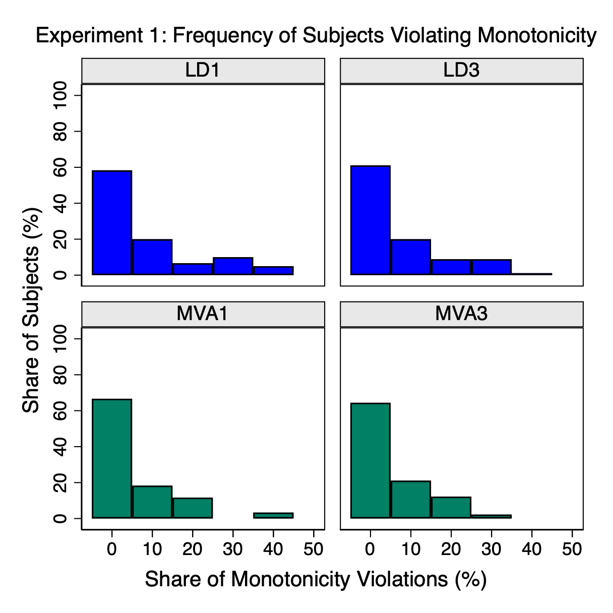
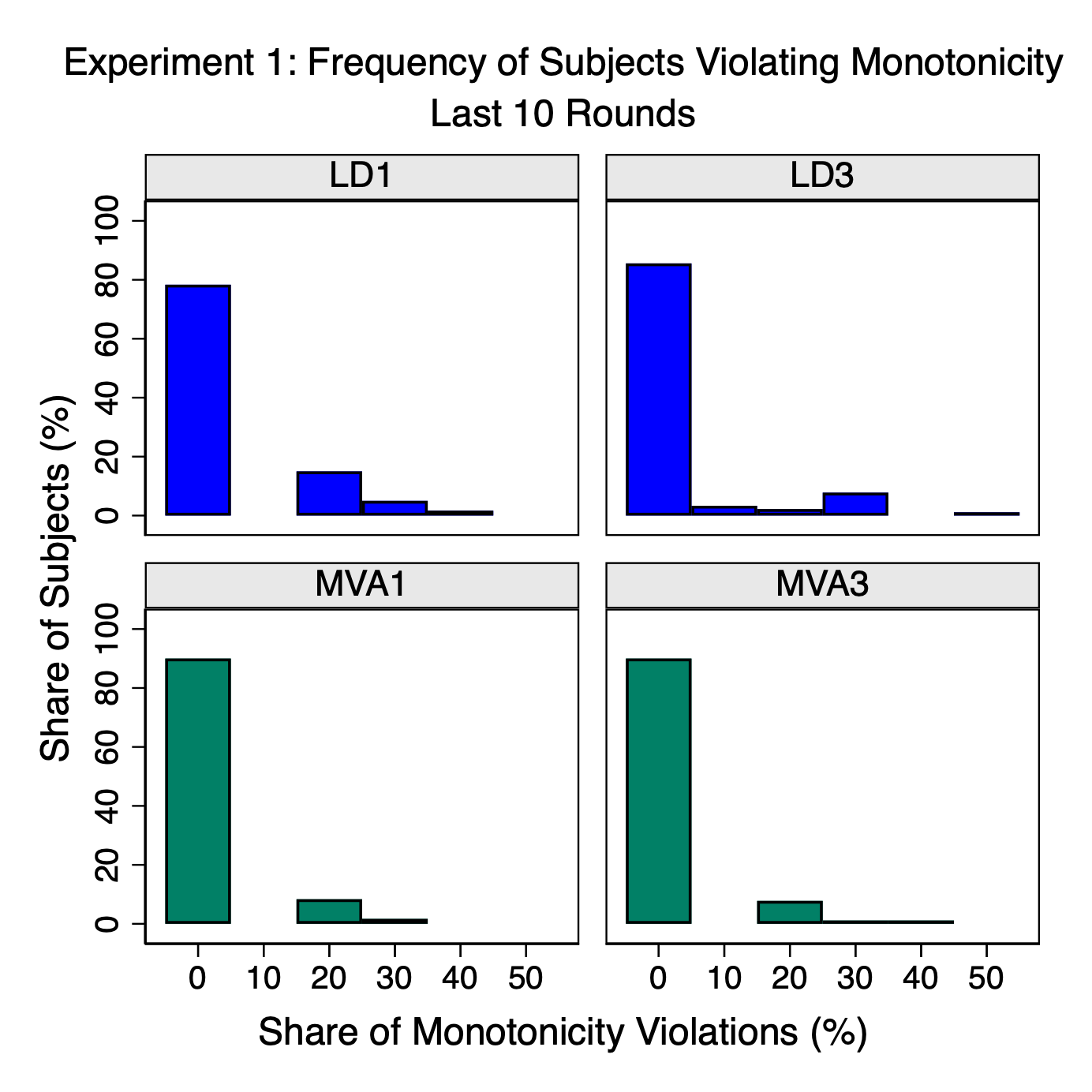
Figure A.1: Monotonicity violations. Histograms. For each subject, we calculate the frequency of violations given the number of rounds played as non-expert. The maximum possible frequency is 50%.

A.2.3 Voting against signal and signal quality

Experiment 1: Frequency of Voting Against Signal.
	(1)	(2)
	Linear Probability	Probit
Signal Precision	-0.407***	-2.058***
	(0.038)	(0.159)
	[0.000]	[0.000]
Round	0.005	0.031
	(0.006)	(0.050)
	[0.457]	[0.535]
LD	-0.006	-0.057
	(0.009)	(0.066)
	[0.504]	[0.390]
N = 15	-0.01	-0.101
	(0.022)	(0.160)
	[0.648]	[0.528]
Second	-0.012	-0.098*
	(0.009)	(0.051)
	[0.216]	[0.056]
Second * Mixed	-0.034	-0.230
	(0.021)	(0.177)
	[0.136]	[0.193]
N = 15 * Second	0.037	0.282
	(0.023)	(0.181)
	[0.132]	[0.120]
N = 15 * Mixed	-0.010	-0.066
	(0.031)	(0.248)
	[0.744]	[0.789]
Constant	0.424***	0.174
	(0.036)	(0.116)
	[0.000]	[0.134]
Observations	2,552	2,552
R-squared	0.154
*** p<0.01, ** p<0.05, * p<0.1

Table A.3: Frequency of voting against signal. Standard errors are clustered at the session level.

Note that the only significant effect is from signal quality (precision). Neither the voting system nor the size of the group matter, but a decrease in signal quality is strongly correlated with an increase in voting against signal. Although voting against signal is an inferior action, the loss from doing so is indeed increasing in signal quality. There could be a small learning effect (voting against signal is less frequent in the treatments run second), but it is quite noisy and counterbalanced by a similarly sized, if statistically insignificant, increase in voting against signal as rounds proceed, possibly from fatigue.

Appendix B Online Appendix

B.1 The bootstrapping procedure: allowing for individual correlation across rounds

Replicating what happens in an individual session, we draw with replacement 15 subjects from the relevant treatment, each with all choices made over the 20 rounds. Among these 15 subjects, we draw, with replacement, 3 subjects, assigning to each of them one choice they made as expert, and 12 subjects, assigning to each one choice made as non-expert. In $N=15$, that constitutes the group and yields one group decision; in $N=5$ treatments, we divide the 12 subjects randomly into three groups of 4 and assign to each group one of the experts drawn earlier, generating three group decisions. We repeat new draws of 3 experts and 12 experts as above 20 times, generating 20 decisions from the same sample of 15 subjects if the treatment has $N=15$, and 60 if the treatment has $N=5$, thus simulating one experimental session. We then draw, always with replacement, a new group of 15 subjects, and repeat the procedure, each time generating 20 (60) decisions from the same group of 15 subjects, depending on the size of the group in the treatment. We repeat the whole procedure 4 times ($N=5$), or 6 times ($N=15$) generating 240 (120) decisions, as in our data from each of the $N=5$ ($N=15$) treatments. We then calculate the frequency of correct decisions, and consider that one data point for that treatment. We repeat the whole process 100,000 times and generate a distribution of the frequency with which the correct decision was reached.

B.2 A short note on beliefs

As reported in the text, at the end of the RDK experiment, we asked: “On average what percentage of trials in the second part do you think you got right?”, and “On average what percentage of trials in the second part do you think the experts got right?” Participants earned 25 cents for replies the fell within 5% of the observed percentage in the group to which the participant was assigned. Figure B.1 plots distributions of the difference between actual own accuracy and the corresponding reported belief, in the left panel, and between actual average experts’ accuracy and the corresponding reported belief, in the panel on the right, for the two different coherence levels. Both panels rely on a single measure of beliefs per subject, and thus the unit of analysis is the subject.

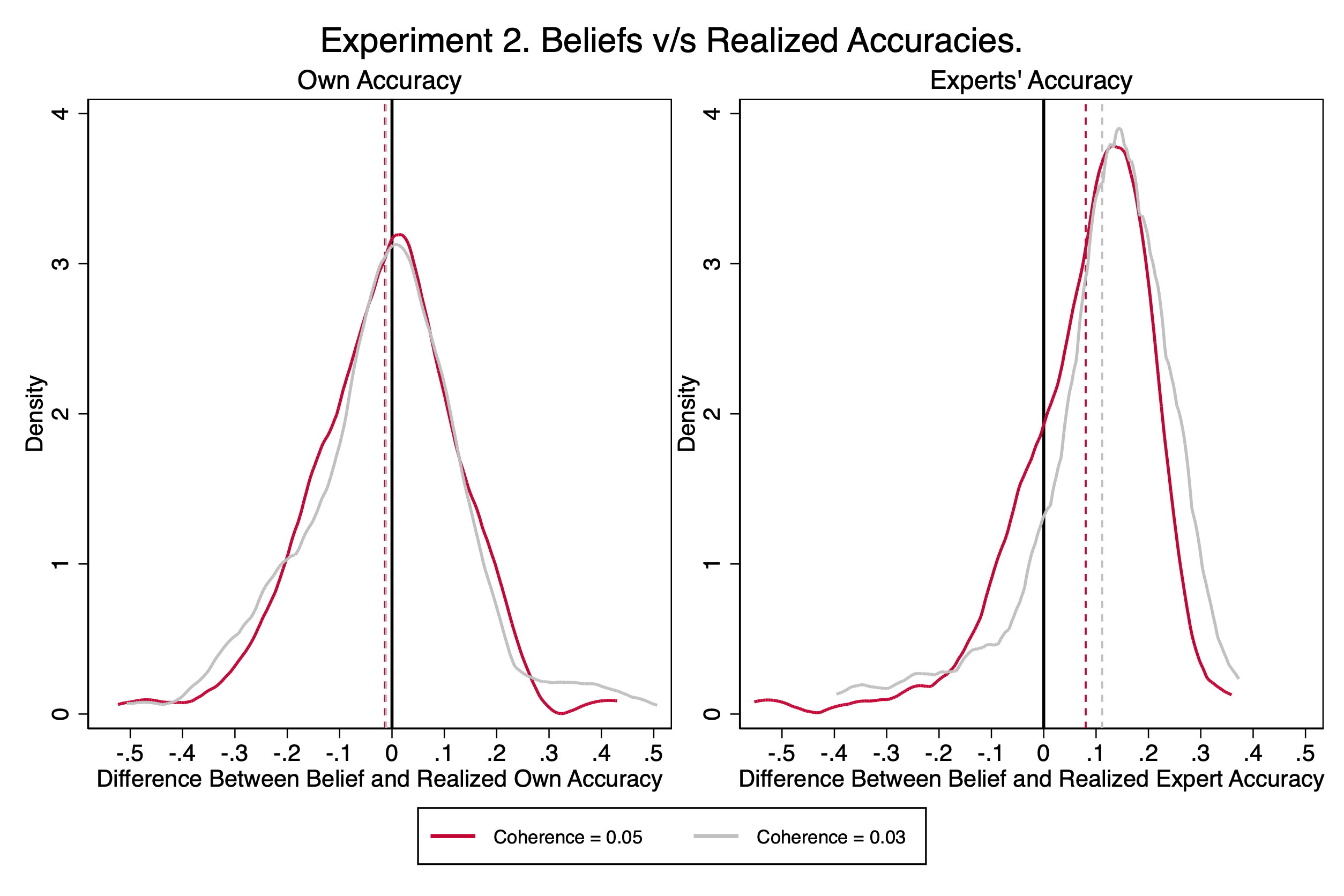
Figure B.1: Difference between actual and reported accuracies. The left panel refers to own accuracy; the right panel to the average of the experts’ accuracy. The vertical lines correspond to the means.

As the figure shows, accuracy of beliefs varies little with coherence. On average, beliefs about own accuracy are remarkably correct, with barely detectable underestimation. The distribution is instead shifted to the right in the case of experts, with about 15% average overestimation, imputable, as we say in the text, to stochasticity in accuracies and reversion to the mean, neglected in the formation of beliefs. Overestimation is somewhat larger at smaller coherence, when the task is more difficult.

Table B.1 reports variants of the regressions in Tables 6 and 7 in the text, now including measures of beliefs. The dependent variable is the frequency of delegation or abstention at the subject level (120 tasks per subject), with data aggregated by coherence level.

Experiment 2: Frequency of Delegation or Abstention.
	(1)	(2)
	Coherence = 0.05	Coherence = 0.03
Own Accuracy	-0.250	-0.0136
	(0.288)	(0.334)
	[0.387]	[0.968]
Experts’ Accuracy	-0.282
	(0.389)
	[0.469]
Belief About Own Accuracy	-0.714***	-0.607***
	(0.144)	(0.161)
	[0.000]	[0.000]
Belief About Experts’ Accuracy	0.337**	0.615***
	(0.160)	(0.181)
	[0.037]	[0.001]
LD	0.249***	0.230***
	(0.0369)	(0.0407)
	[0.000]	[0.000]
Constant	0.757***	0.223
	(0.269)	(0.194)
	[0.005]	[0.252]
Observations	300	250
R-squared	0.184	0.163
*** p<0.01, ** p<0.05, * p<0.1

Table B.1: Beliefs and the decision to delegate/abstain. Expert accuracy is excluded from coherence 0.03 because, with a single group per treatment, it is collinear with LD.

As described in the text, beliefs are strongly significant and have the expected signs but cannot explain the higher tendency towards delegation rather than abstention.

B.3 The Random Dot Kinematogram

In a Random Dot Kinematogram (RDK), the perceptual stimulus consists of a number of dots being displayed on a screen. A proportion of these dots are determined to be signal dots, while the remaining are noise dots. Signal dots all move in a determined direction, while noise dots move at random according to an algorithm. The tasks consists in reporting the direction in which the signal dots are moving. This direction is called the coherent direction and the proportion of signal dots, the coherence, is the main factor in determining the difficulty of the task.

The task can be programmed in various ways, using a variety of parameters (e.g. color, duration, algorithm, number of dots). Research has been done to study the various effects of using different combinations of these parameters (Pilly and Seitz, 2009; Schütz et al., 2010). We take advantage of the recent development of a customizable version of the RDK (Rajananda et al., 2018) which can be implemented as a plugin in jsPsych. This version allows for the configuration of various parameters in order to adjust the task as desired by the researchers. We report in the table below the parameters that we used in our experiment. The reader can find details about how they affect the task in Rajananda et al., 2018 and in the following link: https://www.jspsych.org/6.3/plugins/jspsych-rdk/. It is important to emphasize again that our objective in using the RDK was not to study perception in itself, but rather to create a common task that is reasonably well controlled and calibrated and where, nevertheless, the information about the accuracy of the signals remains ambiguous.

Duration:	1 second
Directions:	Left/Right
Number of dots:	300
Background color:	Black
Color of dots:	White
Dot radius:	2 pixels
Dot movement per frame:	1 pixel
Aperture width:	600 pixels
Aperture height:	400 pixels
Signal selection:	Same
Minimal screen resolutions	1000x600 pixels
Noise type:	Random direction
Aperture shape:	Ellipse
Reinsertion:	Dots reappear randomly when hitting edge
Fixation cross:	No
Aperture border:	No
Coherence:	20% to 3% (according to treatment)

Table B.2: Experiment 2: RDK parameters

References

- [1] Armstrong, Ben and Kate Larson, 2021, “On the Limited Applicability of Liquid Democracy”. Appears at the 3rd Games, Agents, and Incentives Workshop (GAIW2021). Held as part of the Workshops at the 20th International Conference on Autonomous Agents and Multiagent Systems, London, UK, May 2021, IFAAMAS, 7 pages.
- [2] Austen-Smith, David, and Jeffrey Banks, 1996, “Information aggregation, rationality, and the Condorcet Jury theorem”, American Political Science Review, 90:34-45.
- [3] Bhattacharya, Sourav, John Duffy, and Sun-Tak Kim, 2017, “Voting with endogenous information acquisition: Experimental evidence”, Games and Economic Behavior, 102: 316-338.
- [4] Battaglini, Marco, Rebecca Morton, and Thomas Palfrey, 2010, “The swing voter’s curse in the laboratory”, Review of Economic Studies 77:61-89.
- [5] Bahrami, B., K. Olsen, D. Bang, A Roepstorff, G Rees and C. Frith, 2012, “What failure in collective decision-making tells us about metacognition”, Philosophical Transactions of the Royal Society 367: 1350-1365.
- [6] Blum, Christian and Christina Zuber, 2016, “Liquid Democracy: Potentials, Problems, and Perspectives”, Journal of Political Philosophy 24: 162–182.
- [7] Britten K.H., Michael Shadlen, William Newsome, and J. Anthony Movshon, 1992, “The analysis of visual motion: a comparison of neuronal and psychophysical performance”, Journal of Neuroscience 12: 4745–4765.
- [8] Caragiannis, Ioannis and Evi Michas, 2019, “A Contribution to the Critique of Liquid Democracy”, Proceedings of the 28th International Joint Conference on Artificial Intelligence (IJCAI-19), 116-122.
- [9] van de Grind, W.A., A. J. van Doorn, and J. J. Koenderink, 1983, “Detection of coherent movement in peripherally viewed random-dot patterns,” Journal of the Optical Society of America 73: 1674-1683.
- [10] Dhillon, Amrita, Grammateia Kotsialou, and Dimitrios Xefteris, 2021, “Information Aggregation with Delegation of Votes”, Working Paper 2021-22, Quantitative Political Economy Group, King’s College, London.
- [11] Dodgson, Charles, 1884, The Principles of Parliamentary Representation, London: Harrison and Sons.
- [12] Elbittar, Alexander, Andrei Gomberg, Cesar Martinelli, and Thomas R. Palfrey, 2020, “Ignorance and bias in collective decisions”, Journal of Economic Behavior and Organization 174: 332-359.
- [13] Feddersen, Timothy and Wolfgang Pesendorfer, 1996, “The swing voter’s curse”, American Economic Review 86: 408–424.
- [14] Feddersen, Timothy and Wolfgang Pesendorfer, 1997, “Voting Behavior and Information Aggregation in Elections With Private Information”, Econometrica 65: 1029-1058.
- [15] Goeree Jacob and Leeat Yariv, 2011, “An Experimental Study of Collective Deliberation”, Econometrica, 79: 893–921.
- [16] Gölz, Paul, Anson Kahng, Simon Mackenzie, and Ariel D. Procaccia, 2018, “The Fluid Mechanics of Liquid Democracy”, arXiv:1808.01906v1 [cs.GT].
- [17] Green-Armytage, James, 2015, “Direct voting and proxy voting”, Constitutional Political Economy 26:190–220.
- [18] Grofman, Bernard, Guillermo Owen and Scott Feld. 1983. “Thirteen theorems in search of the truth”, Theory and Decision 15:261-278.
- [19] Grofman, Bernard, Guillermo Owen and Scott Feld. 1982. “Evaluating the competence of experts, pooling individual judgments into a collective choice, and delegating decision responsibility to subgroups”. In Felix Geyer and Hans van der Zouwen (Eds.), Dependence and Inequality. NY: Pergamon Press, 221-238.
- [20] Guarnaschelli, Serena, Richard McKelvey and Thomas Palfrey, 2000, “An Experimental Study of Jury Decision Rules”, The American Political Science Review 94: 407-423.
- [21] Goeree Jacob and Leeat Yariv, 2010, “An Experimental Study of Collective Deliberation”, Econometrica 79: 893-921
- [22] Hamman, John, Roberto Weber, and Jonathan Woon, 2011, “An Experimental Investigation of Electoral Delegation and the Provision of Public Goods”, American Journal of Political Science 55: 738-752.
- [23] Hardt, Steve and Lia Lopes, 2015, "Google Votes: A Liquid Democracy Experiment on a Corporate Social Network", Technical Disclosure Commons, http://www.tdcommons.org/dpubs_series/79
- [24] Heer, Jeffrey and Michael Bostock, 2010, “Crowdsourcing Graphical Perception: Using Mechanical Turk to Assess Visualization Design”, CHI 2010: April 10–15, 2010, Atlanta, Georgia, USA: 203-212.
- [25] Kahng, Anson, Simon MacKenzie and Ariel Procaccia, 2018, “Liquid Democracy: An Algorithmic Perspective”, Proceedings of the 32nd AAAI Conference in Artificial Intelligence (AAAI), 1095-1102.
- [26] Margolis, Howard, 1976, “A Note on Incompetence”, Public Choice 26: 119-127.
- [27] Margolis, Howard, 1987, Patterns, Thinking, and Cognition, The Universty of Chicago Press: Chicago, IL.
- [28] McMurray, Joseph, 2013, “Aggregating Information by Voting: The Wisdom of the Experts versus the Wisdom of the Masses”, Review of Economic Studies 80: 277-312.
- [29] McLennan, Andrew, 1998, “Consequences of the Condorcet Jury Theorem for Beneficial Information Aggregation by Rational Agents”, American Political Science Review 92: 413-418.
- [30] Morton, Rebecca and Jean-Robert Tyran, 2011, “Let the experts decide? Asymmetric information, abstention, and coordination in standing committees”, Games and Economic Behavior 72: 485–509.
- [31] Nitzan, Shmuel and Jacob Paroush, 1982, “Optimal decision rules in uncertain dichotomous choice situations”, International Economic Review 23: 289-297.
- [32] Newsome William, K.H. Britten, and J. Anthony Movshon, 1989, “Neuronal correlates of a perceptual decision”, Nature 341: 52–54.
- [33] Pilly, Praveen and Aaron R. Seitz, 2009, “What a difference a parameter makes: A psychophysical comparison of random dot motion algorithms“, Vision Research 49: 1599-1612.
- [34] Rajananda, S., Lau, H. & Odegaard, B., 2018, “A Random-Dot Kinematogram for Web-Based Vision Research”, Journal of Open Research Software 6(1), p.6. doi:10.5334/jors.194.
- [35] Ravindran, Dilip, 2021, “Liquid Democracy”, in Essays in information and behavioral economics, PhD Dissertation, Columbia University, New York, NY.
- [36] Roitman, Jamie and Michael Shadlen, 2002, “Response of neurons in the lateral intraparietal area during a combined visual discrimination reaction time task”, Journal of Neuroscience 22: 9475–9489.
- [37] Rivas, Javier and Friederike Mengel, 2017, “Common value elections with private information and informative priors: theory and experiments”, Games and Economic Behavior 104: 190-221.
- [38] Schütz, Alexander, Doris Braun, J. Anthony Movshon, and Karl Gegenfurtner, 2010, “Does the noise matter? Effects of different kinematogram types on smooth pursuit eye movements and perception”, Journal of Vision, 10(13):26. doi: https://doi.org/10.1167/10.13.26.
- [39] Shapley, Lloyd and Bernard Grofman, 1984, “Optimizing group judgmental accuracy in the presence of interdependencies”, Public Choice 43: 329-343.
- [40] Shubik, Martin, 1970, “On Homo Politicus and the Instant Referendum”, Public Choice 9: 79-84.
- [41] Silver, Ike, Barbara Mellers and Philip Tetlock, 2021, “Wise teamwork: collective confidence calibration predicts the effectiveness of group discussion”, Journal of Experimental Social Psychology, 96: Case Report 104157.
- [42] Sorkin, Robert, Ryan West and Donald Robinson, 1998, “Group Performance Depends on the Majority Rule”, Psychological Science 9: 456-463.
- [43] Sorkin, Robert, Christopher Hays, and Ryan West, 2001, “Signal-Detection Analysis of Group Decision Making”, Psychological Review 108: 183-203.
- [44] Wit, Jőrgen, 1998, “Rational Choice and the Condorcet Jury Theorem”, Games and Economic Behavior 22: 364-376.
- [45] Woods Andy et al., 2015, “Conducting perception research over the internet: a tutorial review”, PeerJ 3:e1058; DOI 10.7717/peerj.1058