Multiple testing under negative dependence

Abstract

The multiple testing literature has primarily dealt with three types of dependence assumptions between p-values: independence, positive regression dependence, and arbitrary dependence. In this paper, we provide what we believe are the first theoretical results under various notions of negative dependence (negative Gaussian dependence, negative regression dependence, negative association, negative orthant dependence and weak negative dependence). These include the Simes global null test and the Benjamini-Hochberg procedure, which are known experimentally to be anti-conservative under negative dependence. The anti-conservativeness of these procedures is bounded by factors smaller than that under arbitrary dependence (in particular, by factors independent of the number of hypotheses tested). We also provide new results about negatively dependent e-values, and provide several examples as to when negative dependence may arise. Our proofs are elementary and short, thus arguably amenable to extensions and generalizations. We end with a few pressing open questions that we think our paper opens a door to solving.

1 Introduction

Ever since the seminal book by [32], the subfield of multiple comparisons and multiple hypothesis testing has grown rapidly and found innumerable applications in the sciences. However, it may be surprising to some practitioners (but not theoreticians working in the field) that some relatively basic questions remain unsolved. For example, the paper by [1] currently has over 90,000 citations (according to Google Scholar in December, 2022), but we have not encountered concrete theoretical results of the performance of the Benjamini-Hochberg (BH) procedure when the p-values are negatively dependent. Closely related to the BH procedure is the Simes global null test, for which we have also not seen results under negative dependence. This paper begins to fill the aforementioned gaps, and paves the way for more progress in this area.

Why has there been a paucity of results on negative dependence? It is certainly not due to shortage of effort: hundreds of the BH citations are by theoretically inclined researchers who did (and still do) think carefully about dependence. We speculate that it is perhaps because there are many definitions of what it means to be “negatively dependent” (and same with positively dependent). Of course in the Gaussian setting, the definitions simply amount to the signs of covariances being positive or negative, but one often cares about more nonparametric definitions that apply more generally, and these are aplenty. It is apriori unclear which definition of dependence will lend itself to (A) analytical tractability for bounding error rates of procedures, (B) have enough examples satisfying the definition so as to potentially yield practical insights in some situations. Once a suitable definition has been adopted, further choices must be made: one must specify whether the dependence is being assumed across all p-values or only those that are null (for example). Finally, the hardest part is of course proving something theoretically valid and practically useful. The multitude of possibilities is daunting, perhaps explaining the lack of progress.

The above combination of (A) and (B) has been arguably successfully achieved for positive dependence. In 1998, [23] published an important result settling the Simes conjecture under a notion of positive dependence called multivariate total positivity of order two, that was studied in depth by [13] in 1980. In 2001, [2] strengthened and extended Sarkar’s result: they showed that the BH procedure controls FDR under a weaker condition called positive regression dependence on a subset (PRDS). This notion too goes back several decades to [15], who proposed PRD in a bivariate context, and (the elder) [24], who generalized PRD to a multivariate context. This paper will provide the first results under the negative dependence analog of the PRD condition.

The aforementioned 2001 paper also proved that under arbitrary dependence, the BH procedure run at target level $\alpha$ on $K$ hypotheses could have its achieved FDR control be inflated a factor of about $\log K$ (sometimes called the Benjamini-Yekutieli or BY correction). This is a huge inflation in modern contexts where $K$ can be in the millions or more. The above results have arguably led to a practical dillema. When the BH procedure is applied in situations where PRDS is a questionable assumption (or is in fact known to not hold), should one apply the aforementioned BY correction? If we do, we know that power will be hurt (a lot). So theoretically one should use the correction, but we have rarely seen the BY correction used in practice.

While we do not disagree with the practice of not using the BY correction, the gap between theory and practice is mildly unsettling. One way out is to seek a better theoretical understanding of what types of assumptions result in inflation factors of much less than $\log K$, along with some justification that these could occur in practice (points (A) and (B) from earlier).

It is in the above context that we see that the current paper makes some novel and arguably important contributions to the literature. Of course, by virtue of being the first, as far as we are aware, nontrivial result on the performance of Simes and BH under negative dependence, it is hopefully a stepping stone for future progress. But equally importantly, the bounds are derived under a very weak notion of negative dependence (and thus easier to satisfy), and the error inflation factors (or anticonservativeness) are proved to be independent of the number of hypotheses $K$, only involving explicit and small constant factors. Thus, the result is not overly pessimistic, and is a stepping stone to bridging theoretical progress with practical advice.

Paper outline.

The rest of this paper is organized as follows. Section 2 presents a few key notions of negative dependence, along with some examples of when they occur. Section 3 presents results on the Simes test using negatively dependent p-values. Section 4 briefly discusses the case of negatively dependent e-values. Section 5 builds on Section 3 to derive results on the FDR of the BH procedure under negative dependence. Section 6 presents some examples, and Section 7 presents simulation results, before we conclude in Section 8.

2 Notions of negative dependence

Fix an atomless probability space $(\Omega,\mathcal{F},\mathbb{P})$ where all random variables live. The aim of this section is to introduce several important notions of negative dependence, summarizing some properties and referencing proofs for the following implications along the way:

We now define all these notions below, from the weakest to the strongest. For a random vector $\mathbf{X}=(X_{1},\dots,X_{K})$, let $F_{k}$ be the distribution function of $X_{k}$ for $k\in\mathcal{K}$. To begin, we say that $\mathbf{X}$ is (lower) weakly negatively dependent if

$$\mathbb{P}\left(\bigcap_{k\in A}\{X_{k}\leq F_{k}^{-1}(p)\}\right)\leq\prod_{k\in A}\mathbb{P}\left(X_{k}\leq F_{k}^{-1}(p)\right)\mbox{~{}~{}~{}for all $A\subseteq\mathcal{K}$ and $p\in(0,1)$}.$$ (1)

We will sometimes write “$X_{1},\dots,X_{K}$ are weakly negatively dependent” instead of “$\mathbf{X}$ is weakly negatively dependent” (also for other notions of dependence), and this should cause no confusion. Upper weak negative dependence can be defined by

$$\mathbb{P}\left(\bigcap_{k\in A}\{X_{k}>F_{k}^{-1}(p)\}\right)\leq\prod_{k\in A}\mathbb{P}\left(X_{k}>F_{k}^{-1}(p)\right)\mbox{~{}~{}~{}for all $A\subseteq\mathcal{K}$ and $p\in(0,1)$},$$ (2)

but we will only need the lower version (1), and so we omit the qualifier “lower” going forward.

Condition (1) is weaker than the notion of negative lower orthant dependence of [3], which is defined by

$$\mathbb{P}\left(\bigcap_{k\in\mathcal{K}}\{X_{k}\leq x_{k}\}\right)\leq\prod_{k\in\mathcal{K}}\mathbb{P}\left(X_{k}\leq x_{k}\right)\mbox{~{}~{}~{}for all $(x_{1},\dots,x_{K})\in\mathbb{R}^{K}$}.$$ (3)

Indeed, we can see that (3) implies (1) by taking $x_{k}\to\infty$ for $k\notin A$ and $x_{k}=x$ for $k\in A$. Further, $\mathbf{X}$ is negative lower orthant dependent if and only if

$$\mathbb{E}\left[\prod_{k=1}^{K}\phi_{k}(X_{k})\right]\leq\prod_{k=1}^{K}\mathbb{E}\left[\phi_{k}(X_{k})\right]\mbox{~{}~{}for all nonnegative decreasing functions $\phi_{1},\dots\phi_{K}$};$$ (4)

see Theorem 6.G.1 (b) of [27] or Theorem 3.3.16 of [18]. All terms like “increasing” and “decreasing” are in the non-strict sense.

There is a related notion of negative upper orthant dependence:

$$\mathbb{P}\left(\bigcap_{k\in\mathcal{K}}\{X_{k}>x_{k}\}\right)\leq\prod_{k\in\mathcal{K}}\mathbb{P}\left(X_{k}>x_{k}\right)\mbox{~{}~{}~{}for all $(x_{1},\dots,x_{K})\in\mathbb{R}^{K}$}.$$ (5)

Similarly to (4), negative upper orthant dependence is equivalent to

$$\mathbb{E}\left[\prod_{k=1}^{K}\phi_{k}(X_{k})\right]\leq\prod_{k=1}^{K}\mathbb{E}\left[\phi_{k}(X_{k})\right]\mbox{~{}~{}for all nonnegative increasing functions $\phi_{1},\dots\phi_{K}$.}$$ (6)

In the series of implications at the start of this section, negative lower orthant dependence (3) can be replaced by negative upper orthant dependence (5), in which case the definition of weak negative dependence in (1) also needs to be altered accordingly (changing $\{X_{k}\leq x\}$ into $\{X_{k}>x\}$).

Negative orthant dependence means that both negative lower orthant dependence and negative upper orthant dependence hold simultaneously.

Negative orthant dependence is in turn weaker than negative association of $\mathbf{X}$, which requires that for any disjoint subsets $A,B\subseteq\mathcal{K}$, and any real-valued, coordinatewise increasing functions $f,g$, we have

$$\text{Cov}(f(\mathbf{X}_{A}),g(\mathbf{X}_{B}))\leq 0,$$ (7)

where $\mathbf{X}_{A}=(X_{k})_{k\in A}$ and $\mathbf{X}_{B}=(X_{k})_{k\in B}$, assuming that $f(\mathbf{X}_{A})$ and $g(\mathbf{X}_{B})$ have finite second moments. Equivalently,

$$\mathbb{E}[f(\mathbf{X}_{A})g(\mathbf{X}_{B})]\leq\mathbb{E}[f(\mathbf{X}_{A})]\mathbb{E}[g(\mathbf{X}_{B})].$$ (8)

This in turn implies that for any non-overlapping sets $\{A_{k}\}_{k=1,\dots,\ell}$ and nonnegative increasing functions $\{\phi_{k}\}_{k=1,\dots,\ell}$, we have

$$\mathbb{E}\left[\prod_{k=1}^{\ell}\phi_{k}(\mathbf{X}_{A_{k}})\right]\leq\prod_{k=1}^{\ell}\mathbb{E}[\phi_{k}(\mathbf{X}_{A_{k}})].$$ (9)

It is necessary and sufficient to require $f$ and $g$ in (7) to be bounded, which can be seen from an approximation argument. For negatively associated random variables, all pairwise correlations are non-positive. Thus, $\mathrm{Var}\left(\sum_{k=1}^{K}X_{k}\right)\leq\sum_{k=1}^{K}\mathrm{Var}(X_{k}).$ [28] proved the following coupling result. Let $X_{1},\dots,X_{K}$ be negatively associated, and let $X^{*}_{1},\dots,X^{*}_{K}$ be independent random variables such that $X_{k}$ and $X^{*}_{k}$ have the same (marginal) distribution for each $k$. Then, for all convex functions $f$, $\mathbb{E}\left[f\left(\sum_{k=1}^{K}X_{k}\right)\right]\leq\mathbb{E}\left[{f\left(\sum_{k=1}^{K}X^{*}_{k}\right)}\right].$

A random vector $\mathbf{X}$ is said to be stochastically decreasing in $Y$ if $\mathbb{E}[g(\mathbf{X})\mid Y=y]$ is decreasing in $y$ whenever $g$ is a coordinatewise increasing function such that the conditional expectation exists. $\mathbf{X}$ is negative regression dependent if

$$\mathbf{X}^{-i} X_{i} i$$ is stochastically decreasing in for every , (10)

where $\mathbf{X}^{-i}$ is the vector formed by deleting the $i$-th coordinate of $\mathbf{X}$. The notion in (10) is called negative dependence through stochastic ordering by [4], and it is the negative analog of the famous positive regression dependence condition (also called positive dependence through stochastic ordering) frequently encountered in multiple testing, under which the Simes test and the Benjamini-Hochberg procedure (both defined later in the paper) are known to be conservative. The term negative regression dependence was used by [15] in case $K=2$.

A random vector $\mathbf{X}$ is Gaussian dependent if there exist increasing functions (or decreasing functions) $f_{1},\dots,f_{K}$ and a Gaussian vector $(Y_{1},\dots,Y_{K})$ such that $X_{k}=f_{k}(Y_{k})$ for $k\in\mathcal{K}$. The correlation matrix of $(Y_{1},\dots,Y_{K})$ is called a Gaussian correlation of $\mathbf{X}$, which is unique if $\mathbf{X}$ has continuous marginals. For instance, if $Y_{1},\dots,Y_{K}$ are standard Gaussian test statistics and $P_{1},\dots,P_{K}$ are the produced one-sided p-values (as $P_{k}=\Phi(-Y_{k})$, where $\Phi$ is the standard Gaussian CDF), then $\mathbf{P}$ is Gaussian dependent. Further, $\mathbf{X}$ is negatively Gaussian dependent if it is Gaussian dependent and its Gaussian correlation coefficients are non-positive ($X_{k}=f_{k}(Y_{k})$ for $k\in\mathcal{K}$):

$$(Y_{1},\dots,Y_{K})\sim\mathrm{N}(\mu,\Sigma),\text{ for some $\mu,\Sigma$ such that }\Sigma_{ij}\leq 0\text{ for all }i\neq j.$$ (11)

If $\mathbf{X}$ is negatively Gaussian dependent, then $\mathbf{X}$ has both negative association and negative regression dependence, implying negative lower orthant dependence and weak negative dependence; see Joag-Dev and Proschan [12, Section 3.4] and also Lemma 5 in Section 3.3. The statement on negative orthant dependence can be verified directly by Slepian’s lemma [30].

Finally, there exists an “extremal (most) negative dependence”: $(X,Y)$ is counter-monotonic if there exists increasing functions $f,g$ and a random variable $Z$ such that $(X,Y)=(f(Z),-g(Z))\text{ almost surely.}$ This can be alternatively stated as $(X(\omega)-X(\omega^{\prime}))(Y(\omega)-Y(\omega^{\prime}))\leq 0$ for almost every pair of $(\omega,\omega^{\prime})\in\Omega^{2}.$ In higher dimensions, a random vector $\mathbf{X}$ is counter-monotonic if each pair of its components is counter-monotonic, that is,

$$(X_{i}(\omega)-X_{i}(\omega^{\prime}))(X_{j}(\omega)-X_{j}(\omega^{\prime}))\leq 0\text{ for almost every $(\omega,\omega^{\prime})\in\Omega^{2}$ and every distinct $i,j$.}$$ (12)

The structure (12) imposes strong conditions on the marginal distributions (in particular, the marginal distributions cannot be continuous when $K\geq 3$). A pairwise counter-monotonic random vector has the smallest joint distribution function among all random vectors with the same marginals. See [20] for the above statements and other forms of extremal negative dependence. As shown by [14], a pairwise counter-monotonic random vector is negatively associated and negative regression dependent.

Closure properties

We mention a few relevant closure properties below.

Monotone transformations: All notions of negative dependence are preserved under concordant coordinatewise monotonic transformations (the term concordant here means that we apply either decreasing transformations to all coordinates or increasing transformations to all coordinates).

Convolution: Suppose that $\mathbf{X}_{1}$ and $\mathbf{X}_{2}$ are independent of each other. If each of $\mathbf{X}_{1}$ and $\mathbf{X}_{2}$ is negative lower orthant dependent, then $\mathbf{X}_{1}+\mathbf{X}_{2}$ is also negative lower orthant dependent; see [17, Theorem 4.2] and [16, Corollary 3]. This also holds for negative association by combining Properties P6 and P7 of [12].

Concatenation: If $\mathbf{X}_{1}$ and $\mathbf{X}_{2}$ are each negatively associated (or negative regression dependent), and are independent of each other, then so is their concatenation $(\mathbf{X}_{1},\mathbf{X}_{2})$.

Marginalization: If $\mathbf{X}$ satisfies any notion of negative dependence mentioned in this section, then so $\mathbf{X}_{A}$ for any nonempty $A\subseteq\mathcal{K}$. This can be verified directly from the definition of these concepts.

Examples of negative dependence

Beyond the Gaussian case mentioned above, some other simple examples may be useful for the reader to keep in mind going forward. These examples can be found in e.g., [12].

Categorical distribution: Suppose that $\mathbf{X}$ is a draw from a categorical distribution with $K$ categories, meaning that it is a binary vector that sums to one. Then $\mathbf{X}$ is counter-monotonic, thus both negatively associated and negative regression dependent.

Multinomial distribution ($m$ balls in $K$ bins): If $\mathbf{X}$ is a draw from a multinomial distribution, meaning that it takes values in $\{0,1\}^{K}$ and $\sum_{i=1}^{K}X_{i}=m$, with each of the $K\choose m$ possibilities being equally likely, then $\mathbf{X}$ is negatively associated as well as negative regression dependent.

Uniform permutations: Let $\mathbf{X}$ be a uniformly random permutation of some fixed vector $(x_{1},\dots,x_{n})$. Then $\mathbf{X}$ is negatively associated.

Sampling without replacement: Along similar lines to the above, sampling without replacement leads to negatively associated random variables. To elaborate: suppose $X_{1},\dots,X_{K}$ are sampled without replacement from a bag containing $N\geq K$ numbers. Then $\mathbf{X}$ is negatively associated.

Recentered Gaussians: [4] pointed out that if $X_{1},\dots,X_{K}$ are iid Gaussians, and $\bar{X}:=(X_{1}+\dots+X_{K})/K$, then $(X_{1}-\bar{X},\dots,X_{K}-\bar{X})$ is multivariate normal with negative correlations, and thus negative regression dependent and negatively associated, for example. They also show that several other examples, like multivariate negative binomial, Dirichlet and multivariate hypergeometric, are all negative regression dependent.

Tournament performance scores: Data summarizing tournament performance are often negatively associated. We summarize some examples below. Consider a round-robin tournament between $K$ players, summarized by a pairwise game matrix $X$ of size $K\times K$. The first three examples below can be shown using Properties P6 and P6 of [12], by noting that the scores $X_{ij}$ and $X_{ji}$ are counter-monotonic, and they are independent of the other scores. Therefore, scores in the $K\times K$ matrix are negatively associated [12, P7], and so are their row sums [12, P6]. The last example is shown by [16].

Binary outcomes. Suppose each game ends in a win or loss. Let $p_{ij}$ denote the probability that $i$ beats $j$ and they play $n_{ij}$ games against each other. Assuming that all games are independent, we have $X_{ij}\sim\text{Binomial}(n_{ij},p_{ij})$. Let us calculate scores of the $K$ players as $S_{i}=\sum_{j\neq i}X_{ij}$, and denote $\mathbf{S}=(S_{1},\dots,S_{K})$. Then $\mathbf{S}$ is negatively associated. (This actually improves a not-so-well known result by [10] who proved $\mathbf{S}$ is negative lower orthant dependent.)

Constant sum games. Suppose at the end of their game(s), each pair of players split a reward $r_{ij}\geq 0$, meaning that the rewards $X_{ij},X_{ji}$ are nonnegative and sum to $r_{ij}$. Defining each player’s scores as before, $S_{i}=\sum_{j\neq i}X_{ij}$, we have that $\mathbf{S}$ is negatively associated. (Obviously this example generalizes the previous one, and even allows for ties.)

Random-sum games. If the aforementioned rewards $r_{ij}$ are themselves random variables, $\mathbf{S}$ remains negatively associated, as long as $(X_{ij},X_{ji})$ is counter-monotonic. This happens in soccer, where the winning team is often awarded three points (and the losing team zero), but if the match is drawn, both teams get one point. This means that $(X_{ij},X_{ji})$ can take the value $(3,0)$, $(1,1)$ or $(0,3)$.

Knockout tournaments. Moving beyond round-robin tournaments to knockout tournaments like in tennis grand slams, let $S_{i}$ denote the total number of games won by player $i$. For example, with 64 players, only the winner $i$ will have $S_{i}=6$, the runner-up $j$ will have $S_{j}=5$, the semifinal losers $k$ will have $S_{k}=4$, and those that lost in the first round have $S_{\ell}=0$. Suppose further that all players are of equal strength, meaning that all outcomes are fair coin flips. For a completely random schedule of matches, $\mathbf{S}$ is negatively associated. For nonrandom draws (such as via player seedings/rankings), $\mathbf{S}$ is negative orthant dependent.

3 Merging negatively dependent p-values

We begin with a recap of some well known properties of the Simes global null test, before turning to the new results under negative dependence.

3.1 Recap: merging p-values with the Simes function

Throughout, $K$ is a positive integer, and $\mathbf{P}=(P_{1},\dots,P_{K})$ is a random vector taking values in $[0,1]^{K}$. Let $\mathbb{P}$ be the true probability measure and write $\mathcal{K}=\{1,\dots,K\}$. Following [33], a p-variable $P$ is a random variable that satisfies $\mathbb{P}(P\leq\alpha)\leq\alpha$ for all $\alpha\in(0,1)$. Let $\mathcal{U}$ be the set of all standard uniform random variables under $\mathbb{P}$.

We first consider the setting of testing a global null. In this setting, we will always assume each of $P_{1},\dots,P_{K}$ is uniformly distributed on $[0,1]$ (thus in $\mathcal{U}$), and this is without loss of generality. Slightly abusing the terminology, we also call $P_{1},\dots,P_{K}$ p-values.

For $p_{1},\dots,p_{K}\in[0,1]$ and $k\in\mathcal{K}$, let $p_{(k)}$ be the $k$-th order statistics of $p_{1},\dots,p_{K}$ from the smallest to the largest. Let $S_{K}:[0,1]^{K}\to[0,1]$ be the Simes function, defined as

$$S_{K}(p_{1},\dots,p_{K})=\bigwedge_{k=1}^{K}\frac{K}{k}p_{(k)},$$

where $a\wedge b:=\min(a,b)$. Applying $S_{K}$ to $\mathbf{P}$ and choosing a fixed threshold $\alpha\in(0,1)$, we obtain the Simes test by rejecting the global null if $S_{K}(\mathbf{P})\leq\alpha$. The type-1 error of this test is $\mathbb{P}(S_{K}(\mathbf{P})\leq\alpha)$.

We begin from the observation that the Simes inequality

$$\mathbb{P}(S_{K}(\mathbf{P})\leq\alpha)\leq\alpha\mbox{~{}~{}~{} for all $\alpha\in(0,1)$}$$ (13)

holds for a wide class of dependence structures of $\mathbf{P}$. It is shown by [29] that if p-values $P_{1},\dots,P_{K}$ are independent or comonotonic (thus identical), then

$$\mathbb{P}(S_{K}(\mathbf{P})\leq\alpha)=\alpha\mbox{ for all $\alpha\in(0,1)$,}$$ (14)

and thus (13) holds as an equality. Moreover, the inequality (13) holds for more general dependence structures; see e.g., [23] and [2]. Let us define the notion of positive regression dependence (PRD). A set $A\subseteq\mathbb{R}^{K}$ is said to be increasing if $\mathbf{x}\in A$ implies $\mathbf{y}\in A$ for all $\mathbf{y}\geq\mathbf{x}$. A random vector $\mathbf{P}$ of p-values is PRD if for any $k\in\mathcal{K}$ and increasing set $A\subseteq\mathbb{R}^{K}$, the function $x\mapsto\mathbb{P}(\mathbf{P}\in A\mid P_{k}\leq x)$ is increasing on $[0,1]$.

Proposition 1 ([2]).

If the vector of p-values $\mathbf{P}$ is PRD, then (13) holds.

If $\mathbf{P}$ is Gaussian dependent (i.e., obtained from jointly Gaussian statistics; see Section 3.3) and its pair-wise correlations are non-negative, then $\mathbf{P}$ satisfies PRD. In this case, (13) holds by Proposition 1. When the correlations are allowed to be negative, things are slightly different: [7] showed that, for $K=2$ and some Gaussian-dependent $\mathbf{P}$ with negative correlation,

$$\mathbb{P}(S_{2}(\mathbf{P})\leq 0.05)\approx 0.0501.$$ (15)

Thus, (13) is slightly violated. The maximum value of $\mathbb{P}(S_{K}(\mathbf{P})\leq\alpha)$ over all possible dependence structures of $\mathbf{P}$ is known ([8]) to be:

$$\max_{\mathbf{P}\in\mathcal{U}^{K}}\mathbb{P}(S_{K}(\mathbf{P})\leq\alpha)=(\ell_{K}\alpha)\wedge 1\mbox{~{}~{}~{} for $\alpha\in(0,1)$,}$$ (16)

where

$$\ell_{K}:=\sum_{k=1}^{K}\frac{1}{k}\approx\log K.$$ (17)

There are several other methods of merging p-values under arbitrary dependence; see [33] and [36]. In this paper, we focus on negatively dependent p-values as well as e-values.

3.2 Simes under negative dependence

We next give a nontrivial upper bound on $\mathbb{P}(S_{K}(\mathbf{P})\leq\alpha)$ when $\mathbf{P}$ is weakly negatively dependent.

Theorem 2 (Additive error bounds).

For every weakly negatively dependent $\mathbf{P}\in\mathcal{U}^{K}$, we have

$$\mathbb{P}(S_{K}(\mathbf{P})\leq\alpha)\leq\alpha+\sum_{k=2}^{K}\binom{K}{k}\left(\frac{\alpha k}{K}\right)^{k}.$$ (18)

We can obtain the more succinct bound that does not depend on $K$,

$$\mathbb{P}(S_{K}(\mathbf{P})\leq\alpha)\leq\alpha+2\alpha^{2}+\frac{9}{2}\alpha^{3}+\frac{1}{\sqrt{8\pi}}\frac{(e\alpha)^{4}}{1-e\alpha}\mbox{~{}~{}~{}~{}for all $\alpha\in(0,1/e)$},$$ (19)

and in particular,

$$\mathbb{P}(S_{K}(\mathbf{P})\leq\alpha)\leq\alpha+2\alpha^{2}+6\alpha^{3}\mbox{~{}~{}~{}for all $\alpha\in(0,0.1].$}$$ (20)

As seen from (20), the bound in Theorem 2 is very close to $\alpha$ when $\alpha$ is close to $0$. Recall from (17) that since $\mathbb{P}(S_{K}(\mathbf{P})\leq\alpha)\leq\ell_{K}\alpha$ under any dependence structure, the bounds above and below can be improved for small $K$ by taking their minimum with $\ell_{K}\alpha$, but we often omit this for clarity. The above bounds also imply the following multiplicative error bounds.

Corollary 3 (Multiplicative error bounds).

For every weakly negatively dependent $\mathbf{P}\in\mathcal{U}^{K}$, we have

$$\mathbb{P}(S_{K}(\mathbf{P})\leq\alpha)\leq 1.26\alpha\text{~{} ~{} ~{} for all }\alpha\in(0,0.1],$$ (21)

and also

$$\mathbb{P}(S_{K}(\mathbf{P})\leq\alpha)\leq 3.4\alpha\text{~{} ~{} ~{} for all }\alpha\in(0,1),$$ (22)

meaning that $(3.4\wedge\ell_{K})S_{K}(\mathbf{P})$ is a p-value for any $K$.

Before we present the proof, a few comments are in order. For $K=2$, the right hand side of (18) becomes $\alpha+\alpha^{2}$, which equals 0.0525 for $\alpha=0.05$. Despite the theorem holding under weakest form of negative dependence, this value is not so far from the empirically observed value in (15) for negative Gaussian dependence. Also, for all practical $\alpha$, the Simes combination results in a valid p-value up to the small constant factor 1.26. However, to formally call it a p-value, the constant is at most 3.4 (though this could potentially be lowered closer to 1 through better approximations).

Proof of Theorem 2 and Corollary 3..

Define $c_{k}=k\alpha/K$ for $k\in\mathcal{K}$. Note that for $k\in\mathcal{K}$, $\{P_{(k)}\leq c_{k}\}=\bigcup_{A\in B_{k}}\bigcap_{j\in A}\{P_{j}\leq c_{k}\}$, where $B_{k}=\{A\subseteq\mathcal{K}:|A|=k\}$ and $|A|$ is the cardinality of $A$. Bonferroni’s inequality gives

$$\mathbb{P}(S_{K}(\mathbf{P})\leq\alpha) =\mathbb{P}\left(\bigcup_{k=1}^{K}\{P_{(k)}\leq c_{k}\}\right)$$

$$\leq\sum_{k=1}^{K}\mathbb{P}\left(P_{(k)}\leq c_{k}\right)=\sum_{k=1}^{K}\mathbb{P}\left(\bigcup_{A\in B_{k}}\bigcap_{j\in A}\{P_{j}\leq c_{k}\}\right).$$

Applying the Bonferroni inequality for every union and (1) for every intersection, we get

$$\mathbb{P}(S_{K}(\mathbf{P})\leq\alpha) \leq\sum_{k=1}^{K}\sum_{A\in B_{k}}\mathbb{P}\left(\bigcap_{j\in A}\{P_{j}\leq c_{k}\}\right)$$

$$\leq\sum_{k=1}^{K}\sum_{A\in B_{k}}\prod_{j\in A}\mathbb{P}(P_{j}\leq c_{k})=\sum_{k=1}^{K}\binom{K}{k}c_{k}^{k}.$$ (23)

This shows (18). Note that, for integers $n\geq k$,

$$\binom{n}{k}=\frac{n!}{k!(n-k)!}=\frac{n(n-1)\dots(n-k+1)}{k!}\leq\frac{n^{k}}{k!}.$$

Stirling’s approximation yields

$$\binom{n}{k}\leq\frac{n^{k}}{k!}\leq\frac{n^{k}}{\sqrt{2\pi k}k^{k}e^{-k}e^{1/(12k+1)}}\leq\frac{n^{k}}{\sqrt{2\pi k}k^{k}e^{-k}}=\frac{1}{\sqrt{2\pi k}}\left(\frac{en}{k}\right)^{k}.$$ (24)

Applying (24) to each term of (3.2) except for the first three terms, we get

$$\mathbb{P}(S_{K}(\mathbf{P})\leq\alpha)$$

$$\leq\alpha+\frac{2(K-1)}{K}\alpha^{2}+\frac{9(K-1)(K-2)}{2K^{2}}\alpha^{3}+\sum_{k=4}^{K}\frac{1}{\sqrt{2\pi k}}\left(\frac{eK}{k}\right)^{k}\left(\frac{k}{K}\alpha\right)^{k}$$

$$=\alpha+\frac{2(K-1)}{K}\alpha^{2}+\frac{9(K-1)(K-2)}{2K^{2}}\alpha^{3}+\sum_{k=4}^{K}\frac{1}{\sqrt{2\pi k}}\left(e\alpha\right)^{k}.$$

$$\leq\alpha+2\alpha^{2}+\frac{9}{2}\alpha^{3}+\sum_{k=4}^{\infty}\frac{\left(e\alpha\right)^{k}}{\sqrt{2\pi k}}.$$ (25)

Therefore, by noting that $\sum_{k=4}^{\infty}\left(e\alpha\right)^{k}={(e\alpha)^{4}}/({1-e\alpha})$ for $\alpha<1/e$, (25) implies the inequality (19), and (20) follows from (19) by direct computation.

Since any probability is no larger than $1$, an upper bound on the probability in (19) for all $\alpha\in(0,1)$ is given by the following function

$$\tilde{s}_{K}(\alpha):=\min\left\{\alpha+2\alpha^{2}+\frac{9}{2}\alpha^{3}+\frac{1}{\sqrt{8\pi}}\frac{(e\alpha)^{4}}{(1-e\alpha)_{+}},1\right\},$$ (26)

where $1/0=\infty$ (i.e., the upper bound is $1$ when $\alpha\geq 1/e$).

By (20), $\tilde{s}_{K}(\alpha)/\alpha\leq 1.26$ for $\alpha\leq 0.1$, and thus the multiplier to correct for negative dependence is at most $1.26$ for relevant values of $\alpha$. We can also verify $\tilde{s}_{K}(\alpha)/\alpha\leq 3.4$ for all $\alpha\in(0,1)$. ∎

The values of $\tilde{s}_{K}(\alpha)$ for common choices of $\alpha\in\{0.01,0.05,0.1\}$, as well as the values of $\alpha$ corresponding to $\tilde{s}_{K}(\alpha)\in\{0.01,0.05,0.1\}$, are given in Table 1. As we can see from the table, the simple formula (20) is a quite accurate approximation of (19).

$\alpha$	0.0098	0.01	0.0454	0.05	0.0830	0.1
$\tilde{s}_{K}(\alpha)$	0.01	0.0102	0.05	0.0556	0.1	0.1260
$\alpha+2\alpha^{2}+6\alpha^{3}$	0.0100	0.0102	0.0501	0.0558	0.1053	0.1260
$\tilde{s}_{K}(\alpha)/\alpha$	1.020	1.020	1.101	1.112	1.205	1.260

Table 1: Values of the upper bounds in Theorem 2

Remark 4.

It is clear from the proof of Theorem 2 that it suffices to require (1) to hold for $p\in[0,\alpha]$ to obtain the upper bound in Theorem 2. That is, we only need weak negative dependence to hold when all components of $\mathbf{P}$ are small than or equal to $\alpha$.

3.3 Negative Gaussian dependence

Theorem 2 leads to upper bounds on the type-1 error of merging weakly negatively dependent p-values using the Simes test. In this section, we discuss the specific situation of Gaussian-dependent p-values, as well as e-values.

For a $K\times K$ correlation matrix $\Sigma$, denote by $\mathcal{G}_{\Sigma}$ the set of all Gaussian-dependent random vectors with Gaussian correlation $\Sigma$. If, $\mathbf{X}\in\mathcal{G}_{\Sigma}$ has standard uniform marginals, then its distribution is called a Gaussian copula (see [19] for copulas).

The following lemma gives a characterization of a few negative dependence concepts for Gaussian-dependent vectors.

Lemma 5.

For Gaussian-dependent $\mathbf{X}\in\mathcal{G}_{\Sigma}$ with continuous marginals, the following statements are equivalent:

1. all off-diagonal entries of $\Sigma$ are non-positive;

2. $\mathbf{X}$ is negatively associated;

3. $\mathbf{X}$ is negative regression dependent;

4. $\mathbf{X}$ is negative orthant dependent;

5. $\mathbf{X}$ is negative lower orthant dependent;

6. $\mathbf{X}$ is weakly negatively dependent.

The implications (i)$\Rightarrow$(ii)$\Leftrightarrow$(iii)$\Leftrightarrow$(iv)$\Leftrightarrow$(v)$\Leftrightarrow$(vi) in Lemma 5 hold true regardless of whether $\mathbf{X}$ has continuous marginals, but (vi)$\Rightarrow$(i) requires this assumption; a trivial counter-example is $\mathbf{X}=(0,\dots,0)$.

Proof.

Since all statements are invariant under strictly increasing transforms, we can safely treat $\mathbf{X}$ as having standard Gaussian marginals (and hence jointly Gaussian). For Gaussian vectors, the implication (i)$\Rightarrow$(ii) is shown by [12], and (i)$\Rightarrow$(iii) is shown by [4]. The implications (ii)$\Rightarrow$(iv)$\Rightarrow$(v)$\Rightarrow$(vi) can be checked by definition; see the diagram in the beginning of Section 2. To see that (vi) implies (i), suppose that an off-diagonal entry $\sigma_{ij}$ of $\Sigma$ is positive (for contradiction). This implies $\mathbb{P}(\{X_{i}\leq 0\}\cap\{X_{j}\leq 0\})>1/4=\mathbb{P}(X_{i}\leq 0)\mathbb{P}(X_{j}\leq 0)$ by direct computation, which violates weak negative dependence. ∎

Suppose that $\mathbf{X}=(X_{1},\dots,X_{K})$ is negatively Gaussian dependent. If a vector of p-values $\mathbf{P}$ is obtained via $\mathbf{P}=(f_{1}(X_{1}),\dots,f_{K}(X_{K}))$ for some decreasing functions (or increasing functions) $f_{1},\dots,f_{K}$, then $\mathbf{P}$ is also negatively Gaussian dependent; the same applies to a vector of e-values $\mathbf{E}$.

A vector of p-values $\mathbf{P}\in\mathcal{G}_{\Sigma}\cap\mathcal{U}^{K}$ is PRD if and only if all entries of $\Sigma$ are non-negative ([2]); it is weakly negatively dependent if and only if all entries of $\Sigma$ are non-positive (Lemma 5). In the above two cases, the type-1 error of the Simes test applied to $\mathbf{P}$ is controlled by Proposition 1 and Theorem 2. For the intermediate case where some entries of $\Sigma$ are positive and some are negative, the type-1 error is much more complicated, and we only have an asymptotic result.

Theorem 6.

For Gaussian-dependent $\mathbf{P}\in\mathcal{G}_{\Sigma}\cap\mathcal{U}^{K}$, the following statements hold.

1. If all off-diagonal entries of $\Sigma$ are non-negative, then

   $$\mathbb{P}(S_{K}(\mathbf{P})\leq\alpha)\leq\alpha\mbox{~{}~{}~{} for all $\alpha\in(0,1)$}$$

2. If all off-diagonal entries of $\Sigma$ are non-positive, then

   $$\mathbb{P}(S_{K}(\mathbf{P})\leq\alpha)\leq\alpha+2\alpha^{2}+6\alpha^{3}\mbox{~{}~{}~{}for $\alpha\in(0,0.1].$}$$

3. It always holds that

   $$\lim_{\alpha\downarrow 0}\frac{1}{\alpha}\mathbb{P}(S_{K}(\mathbf{P})\leq\alpha)\leq 1.$$

Proof.

Statement (i) is well known and it follows from Proposition 1 and the fact that a Gaussian vector with non-negative pair-wise correlations are PRD. Statement (ii) follows from (20) and Lemma 5. To show statement (iii), define the function $M_{-1,K}:(p_{1},\dots,p_{K})\mapsto((p_{1}^{-1}+\dots+p_{K}^{-1})/K)^{-1}$, that is, the harmonic average function. Theorem 2 (ii) of [6] implies $\mathbb{P}(M_{-1,K}(\mathbf{P})\leq\alpha)/\alpha\to 1$, and Theorem 3 of [6] gives $M_{-1,K}\leq S_{K}$. Combining these two statements, we get $\mathbb{P}(S_{K}(\mathbf{P})\leq\alpha)\leq\mathbb{P}(M_{-1,K}(\mathbf{P})\leq\alpha)=\alpha+o(\alpha)$, thus showing statement (iii). ∎

Theorem 6 implies, in particular, that the Simes inequality (13) almost holds for all Gaussian-dependent vectors of p-values and $\alpha$ small enough. It remains an open question to find a useful upper bound for $\mathbb{P}(S_{K}(\mathbf{P})\leq\alpha)$ over all Gaussian-dependent $\mathbf{P}\in\mathcal{U}^{K}$ for practical values of $\alpha$ such as $0.05$ or $0.1$. A simple conjecture is that (20) or a similar inequality holds for all Gaussian-dependent $\mathbf{P}\in\mathcal{U}^{K}$, but a proof seems to be beyond our current techniques.

Remark 7.

Part (iii) of Theorem 6 holds true under the condition that each pair of components of $\mathbf{P}$ has a bivariate Gaussian dependence, which is weaker than Gaussian dependence of $\mathbf{P}$. The claim follows because this condition is sufficient for Theorem 2 (ii) of [6].

Remark 8.

Since the probability $\mathbb{P}(S_{K}(\mathbf{P})\leq\alpha)$ is linear in (distributional) mixtures, the result in Theorem 6 (i) also applies to $\mathbf{P}$ being a mixture of positively Gaussian-dependent vectors of p-values. Similarly, (ii) applies to mixtures of negatively Gaussian-dependent vectors of p-values, and (iii) applies to mixtures of any Gaussian-dependent ones.

3.4 Weighted merging of p-values

Let $\mathbf{w}=(w_{1},\dots,w_{K})\in\mathbb{R}_{+}^{n}$ be a vector of prior weights of p-values, and we assume $w_{1}+\dots+w_{K}=K$; the simplex of such vectors is denoted by $\Delta_{K}$. They may themselves be obtained by e-values from independent experiments; see [11], where the requirement that they add up to $K$ may be dropped (but the terms $\alpha^{2}$ and $\alpha^{3}$ will need some correction). The weighted Simes function is

$$S^{\mathbf{w}}_{K}(p_{1},\dots,p_{K})=\bigwedge_{k=1}^{K}\frac{K}{k}q_{(k)},$$

where $q_{k}=p_{k}/w_{k}$ for $k\in\mathcal{K}$ and $q_{(1)}\leq\dots\leq q_{(K)}$ are the order statistics of $q_{1},\dots,q_{K}$. Clearly, if $w_{1}=\dots=w_{K}=1$, then $S^{\mathbf{w}}_{K}=S_{K}$.

Proposition 9.

For weakly negatively dependent p-values and any $\mathbf{w}\in\Delta_{K}$, the bounds in Theorem 2 hold with $S^{\mathbf{w}}_{K}$ in place of $S_{K}$.

Proof.

It suffices to show that

$$\mathbb{P}(S^{\mathbf{w}}_{K}(\mathbf{P})\leq\alpha)\leq\sum_{k=1}^{K}\binom{K}{k}c_{k}^{k}$$

holds, and the remaining steps follow as in the proof of Theorem 2. Using (3.2) with $P_{1},\dots,P_{K}$ replaced by $P_{1}/w_{1},\dots,P_{K}/w_{K}$, we only need to check the inequality in

$$\sum_{A\in B_{k}}\prod_{j\in A}\mathbb{P}(P_{j}\leq w_{j}c_{k})=\sum_{A\in B_{k}}\prod_{j\in A}(w_{j}c_{k})\leq\binom{K}{k}c_{k}^{k},$$

which holds if

$$\sum_{A\in B_{k}}\prod_{j\in A}w_{j}\leq{\binom{K}{k}}.$$ (27)

Below we show (27). Let $W_{1},\dots,W_{k}$ be random samples from $w_{1},\dots,w_{K}$ without replacement. By definition, we have $\mathbb{E}[W_{1}]=\dots=\mathbb{E}[W_{k}]=1$ and

$$\frac{1}{\binom{K}{k}}\sum_{A\in B_{k}}\prod_{j\in A}w_{j}=\mathbb{E}\left[\prod_{i=1}^{k}W_{i}\right].$$

Since $W_{1},\dots,W_{k}$ are negatively associated (see Section 3.2 of [12]), we have

$$\mathbb{E}\left[\prod_{i=1}^{k}W_{i}\right]\leq\prod_{i=1}^{k}\mathbb{E}\left[W_{i}\right]=1,$$

and hence (27) holds. This is sufficient to obtain the bounds in Theorem 2. ∎

3.5 Iterated applications of negative dependence

A natural question is the following: if $\mathbf{P}$ is negatively dependent, and $A,B$ are two non-overlapping subsets of size $K_{1},K_{2}$, then is it the case that $S_{K_{1}}(\mathbf{P}_{A})$ and $S_{K_{2}}(\mathbf{P}_{B})$ are also negatively dependent? (In what follows, we suppress the subscripts $K_{1}$ and $K_{2}$ for readability.) We cannot settle this question for all definitions of negative dependence, but we can prove the following.

Proposition 10.

If $\mathbf{P}$ is negatively associated, and $\{A_{k}\}_{k=1,\dots,\ell}$ are non-overlapping subsets of $\mathcal{K}$, then $(S(\mathbf{P}_{A_{1}}),\dots,S(\mathbf{P}_{A_{\ell}}))$ is negative orthant dependent. The same result holds for any monotone p-value combination rule (such as Fisher’s, Stouffer’s or Bonferroni, median, average, etc.).

Proof.

Recall the implication of negative association (9). For arbitrary constants $s_{1},\dots,s_{\ell}\geq 0$, choose the coordinatewise increasing nonnegative functions $\phi_{k}$ as $\mathds{1}_{\{S(\mathbf{P}_{A_{k}})>s_{k}\}}$ to yield

$$\mathbb{P}(S(\mathbf{P}_{A_{1}})>s_{1},\dots,S(\mathbf{P}_{A_{\ell}})>s_{\ell})\leq\prod_{k=1}^{\ell}\mathbb{P}(S(\mathbf{P}_{A_{k}})>s_{k}),$$

and this shows negative upper orthant dependence of $(S(\mathbf{P}_{A_{1}}),\dots,S(\mathbf{P}_{A_{\ell}}))$. To obtain negative lower orthant dependence, it suffices to note that (7) holds for componentwise decreasing $f,g$, and thus (9) also holds for non-negative componentwise decreasing functions $\phi_{k}$ chosen as $\mathds{1}_{\{S(\mathbf{P}_{A_{k}})\leq s_{k}\}}$. ∎

The above proposition proves useful in group-level false discovery rate control, as we shall see later. For now, we describe an implication for global null testing with grouped hypotheses in the following corollary.

Corollary 11.

If $\mathbf{P}$ is negatively associated, and $A_{1},\dots,A_{\ell}$ are non-overlapping subsets of $\mathcal{K}$, then

$$\mathbb{P}\Big{(}S(S(\mathbf{P}_{A_{1}}),\dots,S(\mathbf{P}_{A_{\ell}}))\leq\alpha\Big{)}\leq 1.52\alpha\text{ ~{} ~{} for all }\alpha\in[0,0.083),$$

and also

$$\mathbb{P}\Big{(}S(S(\mathbf{P}_{A_{1}}),\dots,S(\mathbf{P}_{A_{\ell}}))\leq\alpha\Big{)}\leq(3.4\wedge\ell_{K})^{2}\alpha\text{ ~{} ~{} for all }\alpha\in[0,1],$$

meaning that $(3.4\wedge\ell_{K})^{2}S(S(\mathbf{P}_{A_{1}}),\dots,S(\mathbf{P}_{A_{\ell}}))$ is a valid p-value. In contrast, if $\mathbf{P}$ is positively regression dependent (PRD), then

$$\mathbb{P}\Big{(}S(S(\mathbf{P}_{A_{1}}),\dots,S(\mathbf{P}_{A_{\ell}}))\leq\alpha\Big{)}\leq\alpha.$$

In the first inequality in Corollary 11, the values $0.083$ and $1.52$ are computed from Table 1 by applying (21) twice. The second inequality is due to the fact that $3.4S(\mathbf{P})$ is a p-value by Theorem 2 under weak negative dependence. The last inequality above was proved by [21, Lemma 2(d)]. Surprisingly, it holds despite the fact that $S(\mathbf{P}_{A_{1}}),\dots,S(\mathbf{P}_{A_{\ell}})$ are not known to themselves be PRD (even though $\mathbf{P}$ is); in fact, the claim under PRD even holds for overlapping groups. It is likely that under certain types of mixed dependence (such as positive dependence within groups but negative dependence across groups, or vice versa), intermediate bounds can be derived.

4 Merging negatively dependent e-values

E-values ([35]) are an alternative to p-values as a measure of evidence and significance. We make a brief but important observation on negatively associated e-values. An e-variable (also called an e-value, with slight abuse of terminology) for testing a hypothesis $H$ is a random variable $E\geq 0$ with $\mathbb{E}^{Q}[E]\leq 0$ for each probability measure $Q\in H$. Further, recall that an e-value may be obtained by calibration from a p-value $P$, i.e., $E=\phi(P)$ for some calibrator $\phi$, which is a nonnegative decreasing function $\phi$ satisfying $\int_{0}^{1}\phi(t)\,\mathrm{d}t\leq 1$ (typically with an equal sign); see [26] and [35].

Theorem 12.

If e-values $E_{1},\dots,E_{K}$ are negatively upper orthant dependent, then $\prod_{i=1}^{k}E_{i}$ is also an e-value for each $k\in\mathcal{K}$. More generally, $E(\boldsymbol{\lambda}):=\prod_{i=1}^{K}(1-\lambda_{i}+\lambda_{i}E_{i})$ is an e-value for any constant vector $\boldsymbol{\lambda}:=(\lambda_{1},\dots,\lambda_{K})\in[0,1]^{K}$. In particular, if the e-values are obtained by calibrating negative lower orthant dependent p-values, then they are negatively upper orthant dependent.

The above proposition is recorded for ease of reference, but its proof is simply a direct consequence of (6). The condition of negative upper orthant dependence in Theorem 12 is weaker than negative orthant dependence or negative association. Thus if $\mathbf{P}$ is Gaussian dependent, and all off-diagonal entries of $\Sigma$ are non-positive, then $E:=\prod_{k=1}^{K}\phi_{k}(P_{k})$ is an e-value for any calibrators $\phi_{1},\dots,\phi_{K}$.

Products are not the only way to combine negatively dependent e-values. The next proposition lays out certain admissible combinations.

Corollary 13.

For negatively upper orthant dependent e-values $E_{1},\dots,E_{K}$, convex combinations of terms

$$\prod_{k\in A}E_{k},\mbox{~{}where $A\subseteq\mathcal{K}$,}$$

are also valid e-values (here the product is $1$ if $A=\varnothing$). This family includes U-statistics of $E_{1},\dots,E_{K}$. Further, such convex combinations, treated as functions from $[0,\infty)^{K}\to[0,\infty)$, are admissible merging functions for negative orthant dependent e-values.

The validity follows because averages of arbitrarily dependent e-values are always e-values. The admissibility follows because these merging functions are admissible within the larger class of merging functions for independent e-values (see [35]).

For independent e-values, [34] observed from simulations that the order-2 U-statistic, defined by

$$U_{2}:=\frac{2}{K(K-1)}\sum_{1\leq k<j\leq K}E_{k}E_{j}$$ (28)

performs quite well in some numerical experiments. Similarly,

$$U_{3}:=\frac{6}{K(K-1)(K-2)}\sum_{1\leq k<j<\ell\leq K}E_{k}E_{j}E_{\ell}$$ (29)

can be useful in different situations. Since $U_{2}$ and $U_{3}$ are both valid e-values under negative upper orthant dependence, we will use these e-values in our simulation examples below.

Note that the Simes combination for e-values, given by

$$S_{K}(e_{1},\dots,e_{K})=\bigvee_{k=1}^{K}\frac{k}{K}e_{[k]},\mbox{~{}where $e_{[k]}$ is the $k$-th largest order statsitic of $e_{1},\dots,e_{K}$,}$$

does result in a valid e-value under arbitrary dependence, but it is uninteresting because it is dominated by the average of the e-values, which is also valid under arbitrary dependence as mentioned above. Thus we only discuss Simes in the context of p-values in this paper.

We end this subsection by presenting an important corollary of Theorem 12 that pertains to the construction of particular e-value that are commonly encountered in nonparametric concentration inequalities. To set things up, following [5], we call a mean-zero random variable $X$ as $v$-sub-$\psi$, if the following condition holds: for every $\lambda\in\mathrm{Domain}(\psi)$, $\mathbb{E}[e^{\lambda X}]\leq e^{\psi(\lambda)v}$, which is simply a bound on its moment generating function. If $X$ is not mean zero, then it is called $v$-sub-$\psi$ if the aforementioned condition is satisfied by $X-\mathbb{E}[X]$. In particular, if $\psi(\lambda)=\lambda^{2}/2$, then $X$ is called $v$-subGaussian. In what follows, we use $n$ instead $K$ for the number of random variables involved, as $n$ here often corresponds to the number of observations instead of the number of tests.

Corollary 14 (Chernoff e-variables).

Suppose $X_{1},\dots,X_{n}$ are negatively associated, and that each $X_{i}$ is $v_{i}$-sub-$\psi_{i}$. Then, denoting by $\mu_{i}:=\mathbb{E}[X_{i}]$, we have that $\exp(\sum_{i=1}^{n}\lambda_{i}(X_{i}-\mu_{i})-\sum_{i=1}^{n}\psi_{i}(\lambda_{i})v_{i})$ is an e-value for any positive constants $\lambda_{1},\dots,\lambda_{n}$ in the domains of $\psi_{1},\dots,\psi_{n}$, respectively.

It is easily checked that if the sub-$\psi$ condition holds only for some subset $\Lambda\subseteq\mathrm{Domain}(\psi)$, then so does the final conclusion. The proof follows directly by invoking Corollary 13 with the e-values $E_{i}:=\exp(\lambda_{i}(X_{i}-\mu)-\psi_{i}(\lambda_{i})v_{i})$.

Such e-values appeared very centrally in the unified framework for deriving Chernoff bounds in [9], and thus we call them Chernoff e-values. As a particular example, assume that for all $i$, we have $\mu_{i}=\mu,~{}v_{i}=v$ and $\psi_{i}(\lambda)=\lambda^{2}/2$, and we also choose $\lambda_{i}=\lambda$. Denoting $\hat{\mu}_{n}:=\sum_{i=1}^{n}X_{i}/n$, we observe that $\exp(n\lambda(\hat{\mu}_{n}-\mu)-nv\lambda^{2}/2)$ is an e-value. Applying Markov’s inequality, we get the claim that

$$\mathbb{P}\left(\hat{\mu}_{n}-\mu>\frac{\log(1/\alpha)}{n\lambda}+v\lambda/2\right)\leq\alpha.$$

Choosing $\lambda=\sqrt{2\log(1/\alpha)/(nv)}$, we get back Hoeffding’s famous inequality for sums (or averages) of subGaussian random variables: $\mathbb{P}(\hat{\mu}_{n}-\mu>\sqrt{{2v\log(1/\alpha)}/{n}})\leq\alpha$, which is known to also hold under negative association.

Other examples of this type can be easily derived, but we omit them for brevity.

5 False discovery rate control

5.1 The BH procedure

In this section, we present an implication of our results in controlling the false discovery rate (FDR). We will obtain an FDR upper bound that may not be very practical. Nevertheless, it is the first result we are aware of that controls FDR under negative dependence (without the Benjamini-Yekutieli corrections of $\approx\log K$ [2]), and hence it represents an important first step that we hope open the door to future work with tighter bounds.

Let $H_{1},\dots,H_{K}$ be $K$ hypotheses. For each $k\in\mathcal{K}$, $H_{k}$ is called a true null if $\mathbb{P}\in H_{k}$. Let $\mathcal{N}\subseteq\mathcal{K}$ be the set of indices of true nulls, which is unknown to the decision maker, and $K_{0}$ be the number of true nulls, thus the cardinality of $\mathcal{N}$. For each $k\in\mathcal{K}$, $H_{k}$ is associated with p-value $p_{k}$, which is a realization of a random variable $P_{k}$. If $k\in\mathcal{N}$, then $P_{K}$ is a p-variable, assumed to be uniform under $[0,1]$. We write the set of such $\mathbf{P}$ as $\mathcal{U}^{K}_{\mathcal{N}}$. We do not make any distribution assumption on $P_{k}$ for $k\in\mathcal{K}\setminus\mathcal{N}$.

A random vector $\mathbf{P}$ of p-values is PRD on the subset $\mathcal{N}$ (PRDS) if for any null index $k\in\mathcal{N}$ and increasing set $A\subseteq\mathbb{R}^{K}$, the function $x\mapsto\mathbb{P}(\mathbf{P}\in A\mid P_{k}\leq x)$ is increasing on $[0,1]$. If $\mathcal{N}=\mathcal{K}$, i.e., all hypotheses are null, then PRDS is precisely PRD. For a Gaussian-dependent random vector $\mathbf{P}$ with Gaussian correlation matrix ${\Sigma}$, it is PRDS if and only if $\Sigma_{ij}\geq 0$ for all $i\in\mathcal{N}$ and $j\in\mathcal{K}$.

A testing procedure $\mathcal{D}:[0,1]^{K}\to 2^{\mathcal{K}}$ reports rejected hypotheses (called discoveries) based on observed p-values. We write $F_{\mathcal{D}}$ as the number of null cases that are rejected (i.e., false discoveries), and $R_{\mathcal{D}}$ as the total number of discoveries truncated below by $1$, that is,

$$F_{\mathcal{D}}=|\mathcal{D}(\mathbf{P})\cap\mathcal{N}|\mbox{~{}~{}~{}and~{}~{}~{}}R_{\mathcal{D}}=|\mathcal{D}(\mathbf{P})|\vee 1.$$

The value of interest is $F_{\mathcal{D}}/R_{\mathcal{D}}$, called the false discovery proportion (FDP), which is the ratio of the number of false discoveries to that of all claimed discoveries, with the convention $0/0=0$ (i.e., FDP is $0$ if there is no discovery; this is the reason of truncating $R_{\mathcal{D}}$ by $1$). [1] introduced the false discovery rate (FDR), which is the expected value of FDP, that is,

$$\mathrm{FDR}_{\mathcal{D}}=\mathbb{E}\left[\frac{F_{\mathcal{D}}}{R_{\mathcal{D}}}\right],$$

where the expected value is taken under the true probability. The BH procedure $\mathcal{D}_{\alpha}$ of [1] rejects all hypotheses with the smallest $k^{*}$ p-values, where

$$k^{*}=\max\left\{k\in\mathcal{K}:\frac{Kp_{(k)}}{k}\leq\alpha\right\}$$

with the convention $\max(\varnothing)=0$, and accepts the rest. For independent ([1]) or PRDS ([2]) p-values, the BH procedure has an FDR guarantee

$$\mathbb{E}\left[\frac{F_{\mathcal{D}_{\alpha}}}{R_{\mathcal{D}_{\alpha}}}\right]\leq\frac{K_{0}}{K}\alpha\mbox{~{}~{}~{} for all $\alpha\in(0,1)$}.$$ (30)

Proposition 15 ([2]).

If the vector of p-values $\mathbf{P}$ is PRDS, then (30) holds. For arbitrarily dependent p-values, the error bound in (30) is inflated by an $\ell_{K}$ factor, similarly to (16).

As a consequence of Proposition 15, for Gaussian-dependent $\mathbf{P}$, (30) holds when the correlations are non-negative. In the setting that all hypotheses are true nulls, i.e., $K_{0}=K$, it holds that

$$\mathbb{E}\left[\frac{F_{\mathcal{D}_{\alpha}}}{R_{\mathcal{D}_{\alpha}}}\right]=\mathbb{P}(|\mathcal{D}_{\alpha}(\mathbf{P})|>0)=\mathbb{P}\left(\bigcup_{k\in\mathcal{K}}\left\{\frac{KP_{(k)}}{k}\leq\alpha\right\}\right)=\mathbb{P}(S_{K}(\mathbf{P})\leq\alpha).$$

Hence, in this setting, the FDR is equal to $\mathbb{P}(S_{K}(\mathbf{P})\leq\alpha)$, and (30) becomes (13). If $P_{1},\dots,P_{K}$ are independent, and the null p-values are uniform on $[0,1]$, then (30) holds as an equality, similar to (14).

5.2 FDR control under negative dependence

We provide an upper bound on the FDR of the BH procedure for weakly negatively dependent p-values, that shows that the error inflation factor is independent of $K$ (unlike Proposition 15). The proof is based on an interesting result in a preprint by [31].

Theorem 16.

If the null p-values are weakly negatively dependent, then the BH procedure at level $\alpha$ has FDR at most $\alpha((-\log\alpha+3.18)\wedge\ell_{K})$.

Technically, the above bound can be improved to $\alpha((-\log\alpha+3.18)\wedge\ell_{K}\tfrac{K_{0}}{K})$, but since $K_{0}$ is unobservable, we omit it above for simplicity. The $\ell_{K}$ multiplier is slightly tighter for small $K$ and $\alpha$, but obviously the overall bound still does not grow with $K$.

Proof.

The $\ell_{K}\alpha$ bound is a consequence of Proposition 15, so we only prove the other part. Theorem 1 of [31] yields

$$\mathrm{FDR}_{\mathcal{D}_{\alpha}}\leq\alpha+\alpha\int_{\alpha}^{1}\frac{\mathrm{FDR}_{0}(x)}{x^{2}}\,\mathrm{d}x,$$ (31)

where $\mathrm{FDR}_{0}(x)$ is the FDR of the BH procedure applied to only the null p-values at level $x$. We will apply the upper bound on $\mathrm{FDR}_{0}(x)$ obtained from Theorem 2. We assume $\alpha\leq 0.3$, because there is nothing to show for the case $\alpha>0.3$ in which the claimed FDR upper bound is larger than $1$. Let $\alpha_{0}=0.3$, which is chosen to be close to $1/e$. Note that

$$\int_{\alpha}^{\alpha_{0}}\frac{1}{x^{2}}\sum_{k=4}^{\infty}\frac{\left(ex\right)^{k}}{\sqrt{2\pi k}}\,\mathrm{d}x =\int_{\alpha}^{\alpha_{0}}\sum_{k=4}^{\infty}\frac{1}{\sqrt{2\pi k}}e^{k}x^{k-2}\,\mathrm{d}x$$

$$=\sum_{k=4}^{\infty}\frac{1}{k-1}\frac{1}{\sqrt{2\pi k}}e^{k}x^{k-1}|_{\alpha}^{\alpha_{0}}$$

$$\leq\sum_{k=4}^{\infty}\frac{1}{k-1}\frac{1}{\sqrt{2\pi k}}e^{k}x^{k-1}|_{0}^{0.3}\approx 0.2473.$$

By applying (25) to (31), and using the above upper bound, we get

$$\mathrm{FDR}_{\mathcal{D}_{\alpha}} \leq\alpha+\alpha\int_{\alpha}^{1}\frac{1}{x^{2}}\min\left\{\left(x+2x^{2}+\frac{9}{2}x^{3}+\sum_{k=4}^{\infty}\frac{\left(ex\right)^{k}}{\sqrt{2\pi k}}\right),1\right\}\,\mathrm{d}x$$

$$\leq\alpha+\alpha\left(\int_{\alpha}^{\alpha_{0}}\frac{1}{x^{2}}\left(x+2x^{2}+\frac{9}{2}x^{3}+\sum_{k=4}^{\infty}\frac{\left(ex\right)^{k}}{\sqrt{2\pi k}}\right)\,\mathrm{d}x+\int_{\alpha_{0}}^{1}\frac{1}{x^{2}}\,\mathrm{d}x\right)$$

$$\leq\alpha+\alpha\left(\int_{\alpha}^{\alpha_{0}}\frac{1}{x}\,\mathrm{d}x+\int_{0}^{\alpha_{0}}\left(2+\frac{9}{2}x\right)\,\mathrm{d}x+0.2474+\int_{\alpha_{0}}^{1}\frac{1}{x^{2}}\,\mathrm{d}x\right)$$

$$\leq\alpha+\alpha\left(\log\alpha_{0}-\log\alpha+1.05+(1/\alpha_{0}-1)\right)$$

$$\leq\alpha\left(-\log\alpha+3.1792\right),$$

and this gives the stated upper bound. ∎

Note that for $K=2$, the Simes error bound was $\alpha+\alpha^{2}$, and so the last calculation simplifies to

$$\mathrm{FDR}_{\mathcal{D}_{\alpha}}\leq\alpha+\alpha\int_{\alpha}^{1}\frac{x+x^{2}}{x^{2}}\,\mathrm{d}x=\alpha+\alpha(1-\alpha)+\log(1/\alpha)=2\alpha+\alpha^{2}-\log\alpha.$$

The values of the $\mathrm{FDR}$ upper bound in Theorem 16 (ignoring the $\ell_{K}$ term) for some values of $\alpha$ are given in Table 2.

$\alpha$	0.00603	0.01	0.01334	0.05	0.1
FDR	0.05	0.07784	0.1	0.3087	0.54812
$\text{FDR}/\alpha$	8.292	7.784	7.502	6.175	5.482

Table 2: Values of the FDR upper bounds in Theorem 16

As seen from Table 2, the upper bound produced by Theorem 16 can be quite conservative in practice, although it is better than the $\ell_{K}$ correction of [2] for large $K$. Recall that, under the stronger condition that the null p-values are iid uniform on $[0,1]$, Theorem 3 of [31] gives an upper bound

$$\mathrm{FDR}_{\mathcal{D}_{\alpha}}\leq\alpha(-\log\alpha+1).$$

Comparing this with the bound $\alpha(-\log\alpha+3.18)$ obtained in Theorem 16, the two bounds share the leading term $\alpha(-\log\alpha)$ for small $\alpha$. Based on the sharpness statement of [31], there is not much hope to substantially improve the FDR bound under the condition of weakly negatively dependent null p-values made in Theorem 16. A remaining open question is to find a better FDR bound with stronger conditions of negative dependence. On the other hand, the e-BH procedure ([37]) controls FDR for arbitrarily dependent e-values, which we will compare with in our simulation results.

5.3 Group-level FDR control

Sometimes, data are available at a higher resolution (say single nucleotide polymorphisms along the genome, or voxels in the brain), but we wish to make discoveries at a lower resolution (say at the gene level, or higher level regions of interest in the brain). This leads to the question of group-level FDR control [21]. The $K$ hypotheses are divided into groups $A,B,C,\dots$. We have p-values for the $K$ individual hypotheses, but wish to discover groups that have some signal without discovering too many null groups (a group is null if all its hypotheses are null, and it is non-null otherwise). In other words, we wish to control the group-level FDR with hypothesis-level p-values.

A natural algorithm for this is to combine the p-values within each group using, say, the Simes combination, and then apply the BH procedure to these group-level “p-values”. We use “p-values” in quotations because while the Simes combination does lead to a p-value under positive dependence (PRDS), as we have seen it only leads to an approximate p-value if the p-values are negatively dependent. Let us call this the Simes+BH_α procedure; to clarify, it applies the BH procedure at level $\alpha$ to the group-level Simes “p-values” formed by applying the Simes combination to the p-values within each group, without any corrections. Then we have the following result.

Proposition 17.

If the p-values are PRDS, the Simes+BH_α procedure controls the group-level FDR at level $\alpha$. If the p-values are negatively associated, the Simes+BH_α procedure controls the group-level FDR at level $3.4\alpha(-\log(3.4\alpha)+3.18)$.

As earlier in the paper, both instances of $3.4$ can be replaced by $3.4\wedge\ell_{K}$, which is tighter for small $K$, but it has been omitted for clarity. The first part of the proposition is a direct consequence of results in Ramdas et al. [21]. The second part simply observes that running the BH_α procedure on Simes “p-values” (that are negative orthant dependent by Proposition 10), is equivalent to running the BH_3.4α procedure on the corrected Simes p-values (the Simes combination multipled by 3.4). We omit the proof.

The FDR bound in Proposition 17, due to repeatedly applying bounds under negative dependence, may be quite conservative in practice. Nevertheless, it is the first result on the group-level FDR control under negative association which does not has an exploding penalty term (compared to the classic BH procedure) as $K\to\infty$, similarly to the case of Theorem 16. Future studies may improve this bound.

6 Examples of negative dependence in testing

We give some examples in testing and multiple comparisons where negative dependence naturally appears. Some details will be supplied in Appendix A.

Example 18 (Tests based on split samples).

Consider a fixed population $\mathbf{x}=(x_{1},\dots,x_{m})\in\mathbb{R}^{m}$, and suppose that $K$ groups of scientists are using samples from the population to test their hypotheses. The p-value (or e-value) for group $k\in\mathcal{K}$ is computed by $f_{k}(\mathbf{x}_{A_{k}})$, where $A_{k}$ is a randomly chosen subset of $\{1,\dots,m\}$ and $f_{k}$ is an increasing function. Since the groups are using different part of the population, $A_{1},\dots,A_{K}$ are disjoint sets. Using Theorem 2.11 of [12], which says that a permutation distribution is negatively associated, we know that the p-values (or e-values) $f_{k}(\mathbf{x}_{A_{k}})$, $k\in\mathcal{K}$, as increasing functions of non-overlapping subsets of negatively associated observations (P6 of [12]), are negatively associated.

Example 19 (Testing the mean of a bag of numbers).

Suppose that the data, represented by the vector $\mathbf{X}=(X_{1},\dots,X_{n})$, are drawn without replacement (uniformly) from a bag of $N$ numbers $x_{1},\dots,x_{N}$, each in $[0,1]$, whose average is $\mu:=\sum_{i=1}^{N}x_{i}/N$. Then, we have seen before that $\mathbf{X}$ is negatively associated. Further, it is clear that $\mathbb{E}[X_{i}]=\mu$ for each $i$. Thus $(1+\lambda(X_{i}-\mu))$ is an e-value for any $\lambda\in[-1,1]$, and by Corollary 13, $\prod_{i=1}^{n}(1+\lambda(X_{i}-\mu))$ is also an e-value. This fact is useful, for example if we want to test $\mu\leq 0.5$ against $\mu>0.5$; in this case, for any $\lambda\in[0,1]$, $\prod_{i=1}^{n}(1+\lambda(X_{i}-0.5))$ is an e-value.

Example 20 (Round-robin tournaments).

Imagine that $K$ players play a round-robin tournament (meaning that each pair of players play some number of games against each other). Suppose that we wish to test the hypotheses that player $k\in\mathcal{K}$ has no advantage or disadvantage over any other players, or the global null hypothesis that all players are equally good. Assume that the game outcomes are independent. Two players being equally good means that whenever they play a game, both players have equal chance of winning or scoring a certain number. Equivalently, since all sports have player rankings or seedings, the global null hypothesis effectively states that these rankings are irrelevant. Let $(X_{ij}^{m})_{i,j\in\mathcal{K},~{}m=1,\dots,M_{ij}}$ be the results of all games, where $M_{ij}$ is the number of games played between player $i$ and player $j$, and $X_{ij}^{m}=-X_{ji}^{m}$. The $k$-th hypothesis is that $X_{kj}^{m}$ is symmetrically distributed around $0$ for all $j$ and $m$. For $k\in\mathcal{K}$, let the p-value or e-value be given by $Y_{k}=f_{k}(X_{kj}^{m}:j\neq k,~{}m=1,\dots,M_{kj})$ for some increasing function $f_{k}$. Then $Y_{1},\dots,Y_{K}$ are negatively associated using P6 of [12]. One way to construct p-values and e-values for this testing problem is described in Appendix A.

Example 21 (Cyclical or ordered comparisons).

Suppose that $X_{1},\dots,X_{K}$ are independent random variables representing scores of $K$ players in a particular order, e.g., pre-tournament ranking. We are interested in testing whether two players adjacent in the list have equal skills. The $k$-th null hypothesis, under some assumptions, $X_{k}$ and $X_{k+1}$ are identically distributed, where we set $X_{K+1}=X_{1}$ but we may safely omit $H_{K}$. For example, for $k\in\mathcal{K}$, a p-value (or e-value) may be obtained in the form $f_{k}(X_{k}-X_{k+1})$ for some increasing function $f_{k}$, since the score differences between two adjacent players are useful statistics. Indeed, we can show a stronger result: For any component-wise increasing functions $h_{k}:\mathbb{R}^{2}\to\mathbb{R}$, $i\in\mathcal{K}$ and independent random variables $X_{1},\dots,X_{K}$, let $Y_{k}=h_{k}(X_{k},-X_{k+1})$, $k\in\mathcal{K}$, where either $X_{K+1}=X_{1}$ or $X_{K+1}$ is independent of $(X_{1},\dots,X_{K})$. Then, the random vector $(Y_{1},\dots,Y_{K})$ is negative orthant dependent. This result is shown in Proposition 22 in Appendix A.

7 Simulations

We now apply our results in Theorems 2, 12 and 16 to global testing or multiple testing problems, and illustrate them by means of several simulation experiments.

7.1 Setting

The test statistics $X_{k},~{}k\in\mathcal{K}$ are generated from correlated z-tests, and they are jointly Gaussian. The null hypotheses are $\mathrm{N}(0,1)$ and the alternatives are $\mathrm{N}(\delta,1)$, where $\delta\geq 0$. Among the $K$ test statistics, $K_{0}$ of them are drawn from the null hypothesis and $K-K_{0}$ of them are from the alternative hypothesis. Let $\pi_{0}=K_{0}/K$ be the proportion of true null hypotheses.

We compute the p-values as

$$P(x):=1-\Phi(x),$$ (32)

where $x\in\{X_{k}:k\in\mathcal{K}\}$; these are the p-values found using the most powerful test given by the Neyman–Pearson lemma. To compute the e-values, we first compute the likelihood ratios,

$$L_{\delta}(x):=\frac{\exp(-(x-\delta)^{2}/2)}{\exp(-x^{2}/2)}=\exp(\delta x-\delta^{2}/2)$$

of the alternative to the null density (which are obviously unit mean under the null, and hence e-values). Since $\delta$ may not be known to the tester, we take an average of $L_{\delta}(x)$ with respect to $\delta$ on $[a,b]$, that is,

$$E(x):=\frac{1}{b-a}\int_{a}^{b}L_{\delta}(x)\,\mathrm{d}\delta={\sqrt{{2\pi}}\exp(x^{2}/2)\left(\Phi(x-a)-\Phi(x-b)\right)}.$$ (33)

Since mixtures of e-values are also e-values, the above is also an e-value. Note that the validity of the p-values and e-values in (32) and (33) only depends on the null hypothesis but not on the alternative hypothesis (but the power depends on reasonably accurate specification of the alternative). As mentioned before, if $(X_{1},\dots,X_{K})$ is negatively Gaussian dependent, then the p-values, as componentwise increasing transforms of $(X_{1},\dots,X_{K})$, are negatively Gaussian dependent. Similarly, the e-values, as componentwise decreasing transforms of $(X_{1},\dots,X_{K})$, are also negatively Gaussian dependent.

7.2 Testing a global null

We first run simulations to test a global null with various methods combining p-values or e-values. We are mainly interested in the methods in this paper under negative dependence, and we will also look at their performance under positive dependence for a comparison. That is, we consider the following settings, and each simulation will be repeated 10,000 times and we report their average.

1. Negative Gaussian dependence: Set the pairwise correlation of $(X_{1},\dots,X_{K})$ to be uniformly chosen between $[-1/(K-1),0]$ in each simulation. For this setting, we consider six different scenarios of $(K,\pi_{0})$: $K\in\{100,1000\}$, corresponding to a small pool and a large pool of hypotheses, and $\pi_{0}\in\{0,50\%,90\%\}$, corresponding to full signal, rich signal, and sparse signal.

2. Positive Gaussian dependence: Set the pairwise correlation of $(X_{1},\dots,X_{K})$ to be uniformly chosen between $[0,1]$ in each experiment. For this setting, we consider two different scenarios of $(K,\pi_{0})$: $K=1000$ and $\pi_{0}\in\{0,50\%\}$, to illustrate some simple comparative observations.

We let $\delta$ vary in $[0,3]$ and the e-values in (33) will be computed with averaging $\delta\in[a,b]=[0,3]$. Fix the type-I error upper bound as $0.05$. We consider the following seven methods:

1. the Simes method with $\ell_{K}$ correction in (16);

2. the Bonferroni correlation (the minimum of p-values times $K$);

3. the Simes method with negative dependence (ND) correction (first row of Table 1);

4. arithmetic mean of of e-values;

5. order-2 U-statistic (U2) of e-values in (28);

6. order-3 U-statistic (U3) of e-values in (29);

7. the product e-value.

All methods based on e-values are compared against the threshold $20$, so that they have a type-I error guarantee of $0.05$. Among these methods, (a), (b) and (d) are valid under arbitrary dependence structures. Method (c) is valid under both negative Gaussian dependence (Theorem 2) and positive Gaussian dependence (implying PRD in Proposition 1). The remaining methods (e), (f) and (g) are valid under negative orthant dependence (Theorem 12).

We plot the rejection probabilities of the above methods in Figure 1 for the setting of negative Gaussian dependence and in Figure 2 for the setting of positive Gaussian dependence.

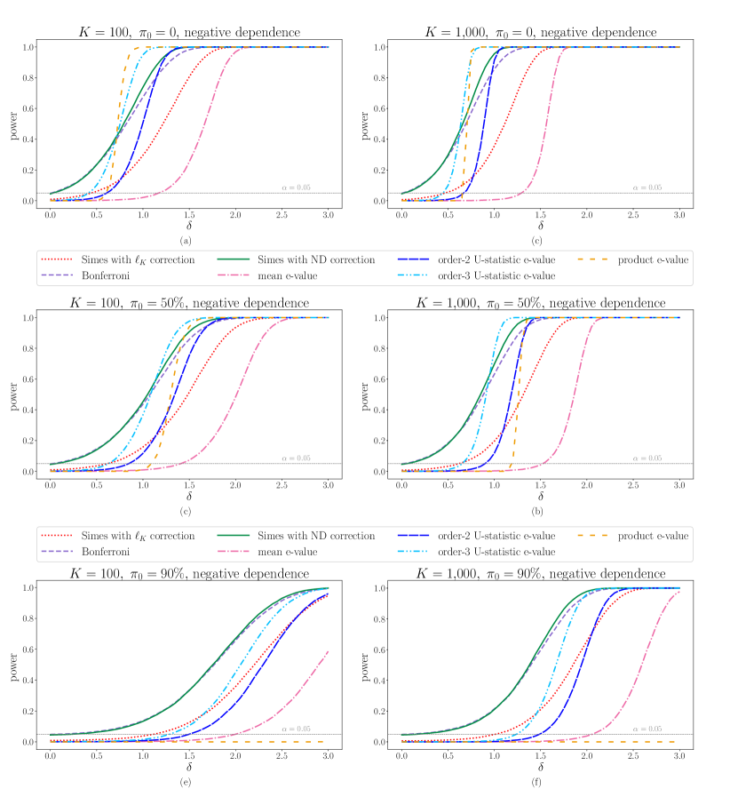
Figure 1: Global null testing (negative Gaussian dependence). All six subplots show power against $\delta$. The left endpoint of $\delta=0$ actually represents the achieved type I error, which appears to be controlled at the nominal level $\alpha=0.05$ for all methods. The key observations are in the text.

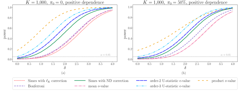
Figure 2: Global null testing (positive Gaussian dependence)

By looking at Figure 1, we make the following observations. The product e-value has strong power when the signal is full ($\pi_{0}=0$), but its performance reduces substantially when the signal is rich ($\pi_{0}=50\%$) or sparse ($\pi_{0}=90\%$). The U3 e-value performs quite well when the signal is full or rich, and loses power when signal is sparse, and the U2 e-value is similar to the U3 e-value with lower power. The Simes method with ND correction performs very well in all cases, and it is similar to the Bonferroni correction in case of sparse signal. The arithmetic average e-value and the Simes method with $\ell_{K}$ correction are not very competitive.

Figure 2 illustrates that the Simes method with ND correction outperforms the Bonferroni correction substantially in the setting of positive dependence; note that both are valid in this setting. On the other hand, although the rejection probabilities of the U2/U3 and product e-values are quite high in Figure 2, they are not theoretically valid in the setting of positive dependence, by noting that $E_{i}E_{j}$ is not an e-value if the e-values $E_{i}$ and $E_{j}$ are positively correlated. The empirical type-I error of the U2/U3 e-values do not seem to exceed the nominal value $0.05$; this is because $1/20$ is practically a conservative bound when applying to e-values.

7.3 Multiple testing procedures with FDR control

Next, we compare multiple testing procedures with FDR control. The setting is similar to the global null testing experiment, but we focus on negative dependence only. Set the pairwise correlation to be $-1/(K-1)$ for $(X_{1},\dots,X_{K})$. Since FDR control is usually applied in large-scale testing, we consider two specifications of $(K,\pi_{0})$: $K=10,000$ or $K=100,000$, and $\pi=80\%$.

We let $\delta$ vary in $[2,4]$ and the e-values in (33) will be computed with averaging $\delta\in[a,b]=[2,4]$. Fix the FDR upper bound as $0.1$. Each simulation will be repeated 1,000 times and we report their average.

The procedures that we compare are:

1. the BH procedure (Section 5.1);

2. the BH procedure with $\ell_{K}$ correction (Section 5.1);

3. the BH procedure with ND correction (first row of Table 2);

4. the e-BH procedure (applying the BH procedure to $1/E$; [37]).

The average numbers of discoveries produced by the four methods are reported in Figure 3. As expected from its definition, none of the other three methods (b), (c) and (d) is as powerful as the BH procedure (a), but the BH procedure without correction does not have a theoretical FDR guarantee under negative dependence. Both BH with $\ell_{K}$ correlation and e-BH are valid under arbitrary dependence, and none of them dominates each other. The BH procedure with ND correction performs better than the other two methods (b) and (d).

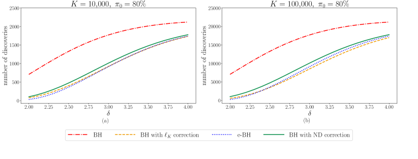
Figure 3: Multiple testing with FDR control (negative Gaussian dependence)

Note that the power comparison between the $\ell_{K}$ correction and the ND correction depends on $K$, because $\ell_{K}$ explodes as $K$ increases but the ND correction is invariant with respect to $K$. Any theoretical improvements to the constants derived in our paper can only further exaggerate the difference between (c) and (b,d).

8 Conclusion

Summary.

This paper provides, to our knowledge, the first bounds for multiple testing methods under negative dependence, in particular the important Simes test and the BH procedure. Some auxiliary results include error bounds for the weighted Simes test, combining negatively dependent e-values, and some implications under negative Gaussian dependence.

Open problems.

The most interesting open problem that remains is to show (what we call) the BH conjecture for negative dependence:

$$\mathbb{E}\left[\frac{F_{\mathcal{D}_{\alpha}}}{R_{\mathcal{D}_{\alpha}}}\right]\leq\frac{K_{0}}{K}\tilde{s}_{K}(\alpha),$$ (34)

for any negatively Gaussian dependent vector of p-values, where $\tilde{s}_{K}(\alpha)$ is in (26). Alternatively, it will be interesting to obtain other multiplicative corrections of $\alpha$, i.e., without involving the term $-\log(\alpha)$ as in Theorem 16.

Recall that most of our results about Simes and the BH procedure involved the weakest form of negative dependence that we defined (some results about e-values required stronger notions, though). A second open problem involves the consideration of whether any of the stronger notions of negative dependence (than weak negative dependence) lead to even better bounds for Simes and BH. Our Theorem 16 assumes weak negative dependence among only null p-values, and it remains unclear whether a better bound can be obtained by assuming some form of negative dependence among all p-values.

Other open problems include extending our results to adaptive Storey-BH-type procedures, to the weighted BH procedure, and to grouped, hierarchical or multilayer settings [21]. We hope to make progress on some of these questions in the future.

Acknowledgments.

We thank Sanat Sarkar for engaging conversations and stimulating suggestions, as well as a missing reference.

Appendix A Details for the examples in Section 6

In this appendix, we first explain the construction of e-values and p-values for the round-robin tournament test in Example 20, and then show the statement in Example 21 on negative orthant dependence for ordered comparison.

One way to test the hypotheses in Example 20 is to first construct e-values for each game, combine them to get e-values for each pair of players, and then combine them further to get e-values for each individual player. Finally, to test the global null, one can combine e-values across all players using the U-statistic of order 2 or 3.

We consider the case where only win, lose and draw are possible outcomes of each game; the case of general scores is similar. Our e-values for a single game are constructed using the principle of testing by betting [25]. To elaborate, imagine that for the $m$-th game between player $i,j$ we have one (hypothetical) dollar at hand. To form the e-value $E^{(m)}_{ij}$ and we bet some fraction $\epsilon\in[0,1]$ that $i$ will beat $j$. If the game is a draw, our wealth remains 1. If we were right, our wealth increases to $1+\epsilon$, and if we were wrong, it decreases to $1-\epsilon$. $E^{(m)}_{ji}$ is constructed in the opposite fashion: so if $E^{(m)}_{ij}=1+\epsilon$, then $E^{(m)}_{ji}=1-\epsilon$; this is the root cause of the resulting negative dependence. Importantly, $\epsilon$ (which could depend on $i,j$, but we omit this for simplicity) must be declared before the game occurs. $E^{(m)}_{ij}$ represents how much we multiplied our wealth due to the $m$-th game and this is an e-value, because under the null hypothesis, there is an equal chance of gaining or losing $\epsilon$, so our expected multiplier equals one.

If a pair of players $i,j$ have played $M_{ij}$ games, let the overall e-value for that pair be defined as $E_{ij}=\prod_{m=1}^{M_{ij}}E^{(m)}_{ij}$. In fact the wealth process across those games forms a nonnegative martingale under the null, since it is the product of independent unit mean terms; however we will not require this martingale property in the current analysis. A large $E_{ij}$ means that player $i$ wins many more games than they lose to $j$.

Let $E_{i}$ denotes the e-value for each player $i\in\mathcal{K}$, that is, $E_{i}=\prod_{j=1,j\neq i}^{K}E_{ij}$. Each $E_{i}$ is an e-value for the same reason as before: it is a product of independent unit mean terms. If $E_{i}$ is large, it reflects that player $i$ more frequently beat other players than lost to them.

Using Properties P1 and P7 of [12], $(E_{ij})_{i,j\in\mathcal{K}}$ is negatively associated because its components are constructed from mutually independent random vectors $(E_{ij},E_{ji})$ and each of these vectors is counter-monotonic (hence negatively associated). We can further see that $(E_{1},\dots,E_{K})$ is also negatively associated, because each $E_{k}$ is an increasing function of $(E_{kj})_{k\in\mathcal{K}}$ (P6 of [12]). Thus, a final e-value for the global null test can be calculated using the U-statistic of order 2 in (28), $E:=\sum_{i<j}E_{i}E_{j}/{K\choose{2}}$, or any other U-statistics as guaranteed by Corollary 13.

Next, we show a result verifying the claim of negative orthant dependence in Example 21.

Proposition 22.

For any component-wise increasing functions $h_{i}:\mathbb{R}^{2}\to\mathbb{R}$, $i\in\mathcal{K}$ and independent random variables $X_{1},\dots,X_{K}$, let $Y_{i}=h_{i}(X_{i},-X_{i+1})$, $i\in\mathcal{K}$, where either $X_{K+1}=X_{1}$ or $X_{K+1}$ is independent of $(X_{1},\dots,X_{K})$. Then, the random vector $(Y_{1},\dots,Y_{K})$ is negative orthant dependent.

Proof.

Note that negative upper orthant dependence is equivalent to (6), and the analogue holds for negative lower orthant dependence by replacing increasing functions with decreasing ones. Hence, it suffices to show

$$\mathbb{E}\left[\prod_{i=1}^{K}f_{i}(X_{i},-X_{i+1})\right]\leq\prod_{i=1}^{K}\mathbb{E}\left[f_{i}(X_{i},-X_{i+1})\right],$$ (35)

for non-negative component-wise increasing functions $f_{1},\dots,f_{K}$, and for non-negative component-wise decreasing functions $f_{1},\dots,f_{K}$. We only show the first case, as the second is similar.

There is nothing to show if $K=1$; we assume $K\geq 2$ in what follows. First, we consider the case $X_{K+1}=X_{1}$. Let $\mathbf{X}^{\prime}:=(X^{\prime}_{1},\dots,X_{K}^{\prime})$ be an independent copy of $\mathbf{X}:=(X_{1},\dots,X_{K})$. Define a function $g:\mathbb{R}^{2K}\to\mathbb{R}$ by

$$g(x_{1},\dots,x_{K},x_{1}^{\prime},\dots,x_{K}^{\prime})=\prod_{i=1}^{K}f_{i}(x_{i},-x_{i+1}^{\prime}).$$

We first claim that for any $(x_{2},\dots,x_{K},x_{2}^{\prime},\dots,x_{K}^{\prime})\in\mathbb{R}^{2K-2}$, it holds that

$$\mathbb{E}[g(X_{1},x_{2},\dots,x_{K},X_{1},x_{2}^{\prime},\dots,x_{K}^{\prime})]\leq\mathbb{E}[g(X_{1},x_{2},\dots,x_{K},X_{1}^{\prime},x_{2}^{\prime},\dots,x_{K}^{\prime})].$$ (36)

To see this, it suffices to observe

$$\mathbb{E}[f_{1}(X_{1},-x_{2})f_{2}(x_{K},-X_{1})]\leq\mathbb{E}[f_{1}(X_{1},-x_{2})f_{2}(x_{K},-X^{\prime}_{1})]$$

due to the Fréchet-Hoeffding (or Hardy-Littlewood) inequality (e.g., [22, Theorem 3.13]) because $f_{1}(X_{1},-x_{2})$ and $f_{2}(x_{K},-X_{1})$ are counter-monotonic. Therefore, (36) holds. It follows that

$$\mathbb{E}[g(\mathbf{X},X_{1},Z_{2},\dots,Z_{K})]\leq\mathbb{E}[g(\mathbf{X},X_{1}^{\prime},Z_{2},\dots,Z_{K})].$$ (37)

holds for all random variables $Z_{1},\dots,Z_{K}$ (here $Z_{1}$ does not appear). Using the above argument on $X_{2}$ we get

$$\mathbb{E}[g(\mathbf{X},Z_{1},X_{2},Z_{3},\dots,Z_{K})]\leq\mathbb{E}[g(\mathbf{X},Z_{1},X_{2}^{\prime},Z_{3},\dots,Z_{K})]$$

holds for all random variables $Z_{1},\dots,Z_{K}$ (here $Z_{2}$ does not appear). Letting $Z_{1}=X_{1}^{\prime}$ we obtain

$$\mathbb{E}[g(\mathbf{X},X_{1}^{\prime},X_{2},Z_{3},\dots,Z_{K})]\leq\mathbb{E}[g(\mathbf{X},X_{1}^{\prime},X_{2}^{\prime},Z_{3},\dots,Z_{K})].$$ (38)

Putting (37) and (38) together we get

$$\mathbb{E}[g(\mathbf{X},X_{1},X_{2},Z_{3},\dots,Z_{K})]\leq\mathbb{E}[g(\mathbf{X},X_{1}^{\prime},X_{2}^{\prime},Z_{3},\dots,Z_{K})].$$

Repeating the above procedure $K$ times we get

$$\mathbb{E}[g(\mathbf{X},\mathbf{X})]\leq\mathbb{E}[g(\mathbf{X},\mathbf{X}^{\prime})],$$

and hence

$$\mathbb{E}\left[\prod_{i=1}^{K}f_{i}(X_{i},-X_{i+1})\right] =\mathbb{E}[g(\mathbf{X},\mathbf{X})]$$

$$\leq\mathbb{E}[g(\mathbf{X},\mathbf{X}^{\prime})]=\prod_{i=1}^{K}\mathbb{E}\left[f_{i}(X_{i},-X^{\prime}_{i+1})\right]=\prod_{i=1}^{K}\mathbb{E}\left[f_{i}(X_{i},-X_{i+1})\right].$$

Therefore, (35) holds.

If we take $f_{K}=1$, then (35) becomes

$$\mathbb{E}\left[\prod_{i=1}^{K-1}f_{i}(X_{i},-X_{i+1})\right]\leq\prod_{i=1}^{K-1}\mathbb{E}\left[f_{i}(X_{i},-X_{i+1})\right]$$

for all independent $X_{1},\dots,X_{K}$. Since $K$ is arbitrary, by moving from $K$ to $K+1$ we obtain that (35) holds for all independent $X_{1},\dots,X_{K+1}$. ∎

References

- Benjamini and Hochberg [1995] Yoav Benjamini and Yosef Hochberg. Controlling the false discovery rate: a practical and powerful approach to multiple testing. Journal of the Royal Statistical Society: Series B (Methodological), 57(1):289–300, 1995.
- Benjamini and Yekutieli [2001] Yoav Benjamini and Daniel Yekutieli. The control of the false discovery rate in multiple testing under dependency. Annals of Statistics, 29(4):1165–1188, 2001.
- Block et al. [1982] Henry W Block, Thomas H Savits, and Moshe Shaked. Some concepts of negative dependence. The Annals of Probability, 10(3):765–772, 1982.
- Block et al. [1985] Henry W Block, Thomas H Savits, and Moshe Shaked. A concept of negative dependence using stochastic ordering. Statistics & Probability Letters, 3(2):81–86, 1985.
- Boucheron et al. [2013] Stéphane Boucheron, Gábor Lugosi, and Pascal Massart. Concentration Inequalities: A Nonasymptotic Theory of Independence. Oxford University Press, 2013.
- Chen et al. [forthcoming, 2023] Yuyu Chen, Peng Liu, Ken Seng Tan, and Ruodu Wang. Trade-off between validity and efficiency of merging p-values under arbitrary dependence. Statistica Sinica, forthcoming, 2023.
- Hochberg and Rom [1995] Yosef Hochberg and Dror Rom. Extensions of multiple testing procedures based on Simes’ test. Journal of Statistical Planning and Inference, 48(2):141–152, 1995.
- Hommel [1983] Gerhard Hommel. Tests of the overall hypothesis for arbitrary dependence structures. Biometrical Journal, 25(5):423–430, 1983.
- Howard et al. [2020] Steven R Howard, Aaditya Ramdas, Jon McAuliffe, and Jasjeet Sekhon. Time-uniform Chernoff bounds via nonnegative supermartingales. Probability Surveys, 17:257–317, 2020.
- Huber [1963] Peter J Huber. A remark on a paper of Trawinski and David entitled: “selection of the best treatment in a paired-comparison experiment”. The Annals of Mathematical Statistics, 34(1):92–94, 1963.
- Ignatiadis et al. [2022] Nikolaos Ignatiadis, Ruodu Wang, and Aaditya Ramdas. E-values as unnormalized weights in multiple testing. arXiv preprint arXiv:2204.12447, 2022.
- Joag-Dev and Proschan [1983] Kumar Joag-Dev and Frank Proschan. Negative association of random variables with applications. The Annals of Statistics, 11(1):286–295, 1983.
- Karlin and Rinott [1980] Samuel Karlin and Yosef Rinott. Classes of orderings of measures and related correlation inequalities. i. multivariate totally positive distributions. Journal of Multivariate Analysis, 10(4):467–498, 1980.
- Lauzier et al. [2023] Jean-Gabriel Lauzier, Liyuan Lin, and Ruodu Wang. Pairwise counter-monotonicity. arXiv preprint arXiv:2302.11701, 2023.
- Lehmann [1966] Erich Leo Lehmann. Some concepts of dependence. The Annals of Mathematical Statistics, 37(5):1137–1153, 1966.
- Malinovsky and Rinott [2022] Yaakov Malinovsky and Yosef Rinott. A note on tournaments and negative dependence. arXiv preprint arXiv:2206.08461, 2022.
- Müller [1997] Alfred Müller. Stochastic orders generated by integrals: a unified study. Advances in Applied probability, 29(2):414–428, 1997.
- Muller and Stoyan [2002] Alfred Muller and Dietrich Stoyan. Comparison Methods for Stochastic Models and Risks. Wiley, 2002.
- Nelsen [2007] Roger B Nelsen. An introduction to copulas. Springer Science & Business Media, 2007.
- Puccetti and Wang [2015] Giovanni Puccetti and Ruodu Wang. Extremal dependence concepts. Statistical Science, 30(4):485–517, 2015.
- Ramdas et al. [2019] Aaditya K Ramdas, Rina F Barber, Martin J Wainwright, and Michael I Jordan. A unified treatment of multiple testing with prior knowledge using the p-filter. The Annals of Statistics, 47(5):2790–2821, 2019.
- Ruschendorf [2013] Ludger Ruschendorf. Mathematical Risk Analysis: Dependence, Risk Bounds, Optimal Allocations and Portfolios. Springer, 2013.
- Sarkar [1998] Sanat K Sarkar. Some probability inequalities for ordered MTP2 random variables: a proof of the Simes conjecture. Annals of Statistics, 26(2):494–504, 1998.
- Sarkar [1969] Tapas K Sarkar. Some lower bounds of reliability. Technical report, Stanford University, Department of Statistics, 1969.
- Shafer [2021] Glenn Shafer. Testing by betting: A strategy for statistical and scientific communication. Journal of the Royal Statistical Society: Series A (Statistics in Society), 184(2):407–431, 2021.
- Shafer et al. [2011] Glenn Shafer, Alexander Shen, Nikolai Vereshchagin, and Vladimir Vovk. Test martingales, Bayes factors and p-values. Statistical Science, 26(1):84–101, 2011.
- Shaked and Shanthikumar [2007] Moshe Shaked and J George Shanthikumar. Stochastic Orders. Springer, 2007.
- Shao [2000] Qi-Man Shao. A comparison theorem on moment inequalities between negatively associated and independent random variables. Journal of Theoretical Probability, 13(2):343–356, 2000.
- Simes [1986] R John Simes. An improved Bonferroni procedure for multiple tests of significance. Biometrika, 73(3):751–754, 1986.
- Slepian [1962] David Slepian. The one-sided barrier problem for Gaussian noise. Bell System Technical Journal, 41(2):463–501, 1962.
- Su [2018] Weijie J Su. The FDR-linking theorem. arXiv preprint arXiv:1812.08965, 2018.
- Tukey [1953] John Wilder Tukey. The problem of multiple comparisons. Technical Report, Princeton University, 1953.
- Vovk and Wang [2020a] Vladimir Vovk and Ruodu Wang. Combining p-values via averaging. Biometrika, 107(4):791–808, 2020a.
- Vovk and Wang [2020b] Vladimir Vovk and Ruodu Wang. True and false discoveries with independent e-values. arXiv preprint arXiv:2003.00593, 2020b.
- Vovk and Wang [2021] Vladimir Vovk and Ruodu Wang. E-values: Calibration, combination and applications. The Annals of Statistics, 49(3):1736–1754, 2021.
- Vovk et al. [2022] Vladimir Vovk, Bin Wang, and Ruodu Wang. Admissible ways of merging p-values under arbitrary dependence. The Annals of Statistics, 50(1):351–375, 2022.
- Wang and Ramdas [2022] Ruodu Wang and Aaditya Ramdas. False discovery rate control with e-values. Journal of the Royal Statistical Society, Series B, 84(3):822–852, 2022.