A Natural Bias for Language Generation Models

Abstract

After just a few hundred training updates, a standard probabilistic model for language generation has likely not yet learnt many semantic or syntactic rules of natural language, making it difficult to estimate the probability distribution over next tokens. Yet around this point, these models have identified a simple, loss-minimising behaviour: to output the unigram distribution of the target training corpus. The use of such a heuristic raises the question: Can we initialise our models with this behaviour and save precious compute resources and model capacity? Here we show that we can effectively endow standard neural language generation models with a separate module that reflects unigram frequency statistics as prior knowledge, simply by initialising the bias term in a model’s final linear layer with the log-unigram distribution. We use neural machine translation as a test bed for this simple technique and observe that it: (i) improves learning efficiency; (ii) achieves better overall performance; and perhaps most importantly (iii) appears to disentangle strong frequency effects by encouraging the model to specialise in non-frequency-related aspects of language.

1 Introduction

Consider the structure of a number of core tasks in natural language processing (NLP): predicting the next word following a given context. What if you did not understand the context – for example, if you did not know the language? In the absence of such knowledge, the optimal prediction would be the language’s most frequent word. In fact, optimally one would predict each word according to its (unigram) frequency. This is precisely the strategy that neural language models have been empirically observed to employ during early training stages Chang and Bergen (2022) – before they have learnt a language’s syntax or semantics.

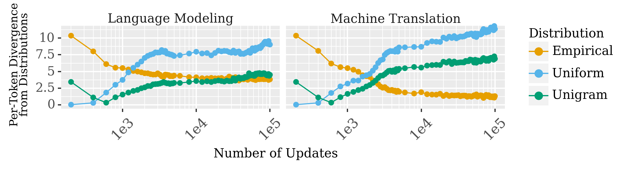
Figure 1: Average per-token divergence of the model from unigram, uniform, and empirical distributions of respective training set as a function of training step (log-scale). Early in training, the model output closely matches the unigram distribution for all contexts.

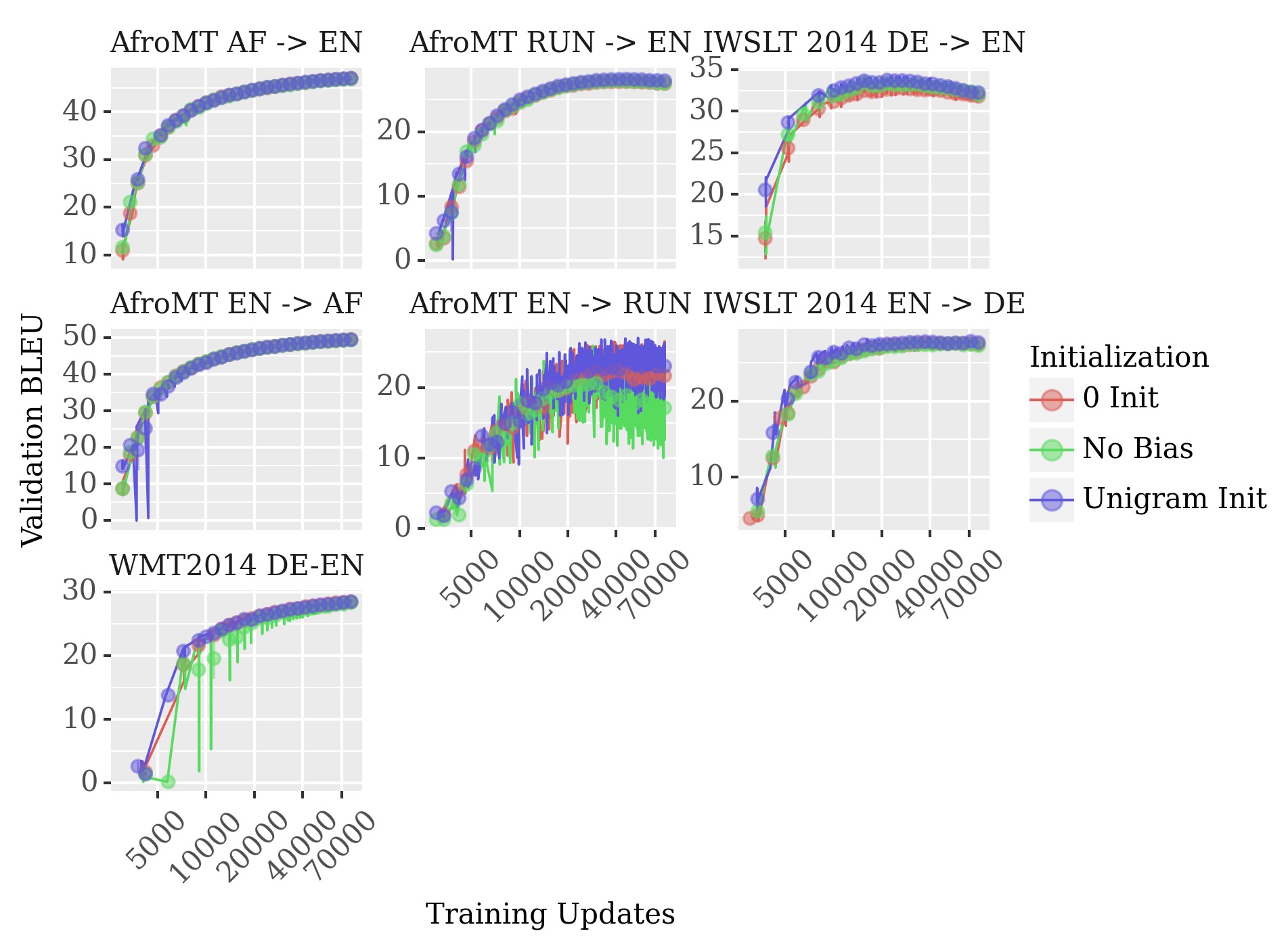
Figure 5: Validation BLEU over the course of training. $y$-axis is on log-scale.

Although this strategy of predicting the unigram distribution emerges early in training, it still takes the model hundreds (or even thousands) of parameter updates to learn it from a cold start (see Fig. 1 or Chang and Bergen, 2022, Fig. 5). Yet a straightforward factorisation of a language model’s final linear layer shows that we can in fact encode this frequency-related knowledge prior to any optimisation, with the goal of bypassing this early stage of learning: Concretely, this is done by setting the bias term in a model’s final linear layer to the log-unigram distribution of the training data. Mathematically, this setup can be loosely interpreted as a modular “product of experts” (Hinton, 2002), where the bias term represents a simple unconditional distribution over the vocabulary, thus allowing the input-dependent logits to specialise in capturing contextual information. Indeed, we argue that a more modular design that disentangles word-frequency effects from contextual information may be desirable, given the recently-observed negative effects of word frequency statistics on models’ generalisation abilities Wei et al. (2021); Puccetti et al. (2022); Rajaee and Pilehvar (2022).

While this initialisation approach has been historically used in language models (Mnih and Hinton, 2007; Botha and Blunsom, 2014; Fang et al., 2015, inter alia), it has not seen widespread adoption within our current language generation architectures – an observation we attribute to uncertainty around whether the bias term automatically specialises to capture frequency without explicit encouragement to do so. We first observe that this is not the case – in fact, the final-layer bias term rarely changes from its random initialisation (see § A.6), suggesting frequency is encoded elsewhere in the model parameters. We then empirically explore the impact of this initialisation on various aspects of model behaviour – within the context of current Transformer models for machine translation – including overall performance, learning efficiency, and the relationship between model-assigned probability and word frequency. We find this initialisation indeed leads to increased training efficiency: models achieve higher bleu scores earlier on in training. More surprisingly, it also leads to improved overall performance. We discuss several potential reasons for these results, including changes to training dynamics and a mitigation of overfitting to surface statistics.

2 Probabilistic Language Generators

2.1 Preliminaries

We consider neural probabilistic models $p_{\scaleto{{\boldsymbol{\theta}}}{4pt}}$ for language generation. While there are a variety of architectural choices that can be made, most are autoregressive and follow a local-normalisation scheme. Explicitly, given prior context $\mathbf{y}_{<t}\mathrel{\stackrel{{\scriptstyle\textnormal{def}}}{{=}}}\langle y_{0},\dots,y_{t-1}\rangle$, these models output a probability distribution $p_{\scaleto{{\boldsymbol{\theta}}}{4pt}}(\cdot\!\mid\!\mathbf{y}_{<t})$ over the next token $y\in\overline{\mathcal{V}}\mathrel{\stackrel{{\scriptstyle\textnormal{def}}}{{=}}}\mathcal{V}\cup\{\textsc{eos}\}$, where $\mathcal{V}$ is the model’s predefined vocabulary and eos is a special end-of-sequence token. To ensure that $p_{\scaleto{{\boldsymbol{\theta}}}{4pt}}$ provides a valid probability distribution, the output of the model is projected onto the probability simplex $\Delta^{|\overline{\mathcal{V}}|-1}$ using a softmax transformation after a (learnt) linear projection layer:

$$p_{\scaleto{{\boldsymbol{\theta}}}{4pt}}(y\!\mid\!\mathbf{y}_{<t}) =\mathrm{softmax}\left(\mathbf{W}\,\boldsymbol{\phi}(\mathbf{y}_{<t})+\mathbf{b}\right)_{y}$$ (1)

$$\mathrel{\stackrel{{\scriptstyle\textnormal{def}}}{{=}}}\frac{e^{\mathbf{W}_{y}\,\boldsymbol{\phi}(\mathbf{y}_{<t})+\mathrm{b}_{y}}}{\sum_{y^{\prime}\in\overline{\mathcal{V}}}e^{\mathbf{W}_{y^{\prime}}\,\boldsymbol{\phi}(\mathbf{y}_{<t})+\mathrm{b}_{y^{\prime}}}}$$ (2)

where $\mathbf{W}\in\mathbb{R}^{|\overline{\mathcal{V}}|\times d}$ denotes a weight matrix, $\mathbf{b}\in\mathbb{R}^{|\overline{\mathcal{V}}|}$ a bias vector, and $\boldsymbol{\phi}:\mathcal{V}^{*}\rightarrow\mathbb{R}^{d}$ the model’s $d$-dimensional encoding for a given context.

A number of prior studies have investigated whether – and if so, at what stage during the learning process – NLP models learn various linguistic phenomena (Alain and Bengio, 2017; Adi et al., 2017, inter alia). Among the key findings are that language models reflect the statistical tendencies exhibited by their respective training corpora Takahashi and Tanaka-Ishii (2017, 2019); Meister and Cotterell (2021); some of which are learnt early on in training (Liu et al., 2021). For example, Chang and Bergen (2022) observe that, after only $\sim 1000$ training updates, language models’ outputs are approximately equal to the unigram distribution, regardless of the context that they condition on. We similarly observe this for machine translation models (see Fig. 1).

2.2 A Natural Bias

These learning trends motivate trying to supply language generation models with a natural starting point: the unigram distribution. Fortunately, this form of prior knowledge can be modularly encoded in standard neural models using the bias term of the final, pre-softmax linear layer. Consider the standard operation for projecting the output of the model onto the probability simplex. Upon closer inspection, we see that eq. 2 has an interpretation as the product of two probability distributions, up to a normalisation constant:

$$p_{\scaleto{{\boldsymbol{\theta}}}{4pt}}(\cdot\!\mid\!\mathbf{y}_{<t}) \propto e^{\mathbf{W}\,\boldsymbol{\phi}(\mathbf{y}_{<t})}\cdot e^{\mathbf{b}}$$ (3)

$$\propto p_{\scaleto{\mathbf{W}\boldsymbol{\phi}}{4pt}}(\cdot\!\mid\!\mathbf{y}_{<t})\cdot p_{b}(\cdot)$$ (4)

i.e., one described by $p_{\scaleto{\mathbf{W}\boldsymbol{\phi}}{4pt}}(\cdot\!\mid\!\mathbf{y}_{<t})$ – which is contextual as it depends on the input $\mathbf{y}_{<t}$ – and a separate, non-contextual term denoted by $p_{b}(\cdot)$. Thus, we can qualitatively view this setup as factorising the model’s prediction into these two components. In this light, it makes intuitive sense that $p_{b}$ should be the unigram distribution – a distribution which optimally predicts (w.r.t. negative log-likelihood loss) the next-token when there is no contextual information to condition on. Note that such a setup – where a probability distribution is modelled using a product of several simpler distributions, each of which can specialise on modelling one aspect of the problem – is referred to as a product of experts Hinton (2002).

3 Related Work

As previously mentioned, prior work has likewise taken advantage of the interpretation of the bias term as a frequency offset when initialising model parameters (Mnih and Hinton, 2007; Botha and Blunsom, 2014; Fang et al., 2015, inter alia). Yet such techniques have fallen to the wayside for a number of years now, as other more prominent determinants of model performance and training efficiency have dominated the community’s attention. We revisit this initialisation strategy in the context of today’s neural language models.

The practice of directly incorporating unigram probabilities into next-word predictions can be likened to the back-off methods proposed in the $n$-gram literature Kneser and Ney (1995); Chen and Goodman (1999). Indeed, there is an entire class of methods built around learning deviations from some base reference distribution, some of which have been employed specifically for language modelling Berger and Printz (1998); Teh (2006); Grave et al. (2017). More recently, Li et al. (2022) cast neural language modelling as the learning of the residuals not captured by $n$-gram models and Baziotis et al. (2020) use language models as a reference distribution for training low resource machine translation models.

Another class of prior work has similarly explored efficient strategies for model weight initialisation (Glorot and Bengio, 2010; Le et al., 2015; Mu et al., 2018, inter alia), including random variable choices and re-initialisation criterion. In a similar vein, Ben Zaken et al. (2022) investigate the usefulness of the bias term, albeit for efficient fine-tuning techniques. They show that, often, modifying solely the bias parameters during fine-tuning provides comparable performance to updating the entire model. Both our results thus showcase the usefulness of this simple set of parameters for natural language processing tasks.

Other works have also embraced frameworks akin to product or mixture of experts in language modelling or generation tasks. For example Neubig and Dyer (2016) combine neural and count-based language models in a mixture of experts paradigm; Artetxe et al. (2022) take advantage of the mixture of experts structure to propose a compute-efficient language modelling architecture. In contrast, we suggest a simple initialisation method that does not require training additional models or major changes to model architectures.

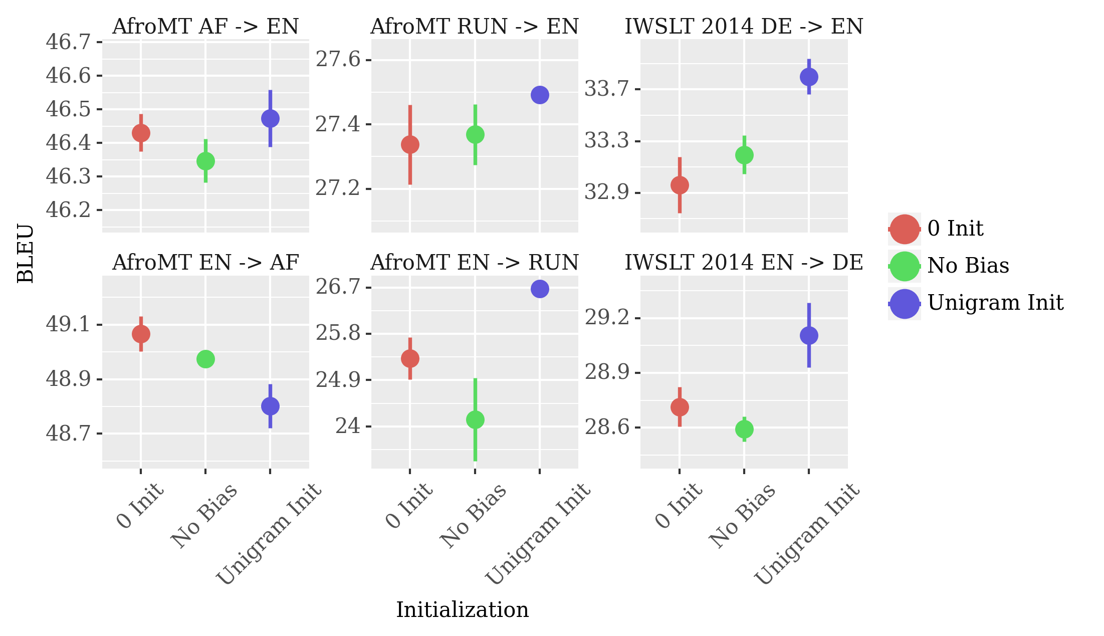
Figure 2: Mean test bleu for models with different bias initialisations. Bars indicate standard error. Panes are adjusted so that the $y$-axis spans at least $0.5$ bleu.

4 Experiments

We explore the effects of the unigram bias initialisation strategy on neural machine translation systems in comparison to a standard initialisation technique: initialising the bias to all $0$s (denoted as $\overset{\rightarrow}{0}$) or omitting the bias term entirely.

4.1 Setup

We perform experiments with several language pairs: WMT’14 German-to-English (De$\rightarrow$En; Bojar et al., 2014), IWSLT’14 German-to-English (De$\leftrightarrow$En; Cettolo et al., 2012), and Afrikaans/Rundi-to-English in the AfroMT dataset (Run$\leftrightarrow$En and Af$\leftrightarrow$En; Reid et al., 2021). These corpora span several language families and different sizes to demonstrate performance in higher, medium and lower resource domains ($\sim\!\!4.5$M, $\sim 750$K and $\sim 150$K sentence pairs, respectively). All models use the standard Transformer encoder–decoder architecture Vaswani et al. (2017), with 6 layers in both. The IWSLT and AfroMT Run$\leftrightarrow$En models have 4 attention heads per layer (adjusted for the smaller size of these datasets) while all other models have 8 attention heads. Dropout is set to $0.1$; the feedforward hidden dimension is set to 512 for the WMT model and 256 for all other models. Parameter estimation is performed using stochastic gradient-descent techniques, with the standard maximum likelihood objective and label smoothing Szegedy et al. (2015) with hyperparameter $\alpha=0.1$. We use the Adam optimizer Kingma and Ba (2015) with $(\beta_{1},\beta_{2})=(0.9,0.997)$. Early stopping was performed during training, i.e., model parameters were taken from the checkpoint with the best validation set bleu Papineni et al. (2002).

We preprocess the data using subword tokenisation with the SentencePiece library Kudo and Richardson (2018)author=tiago,color=cyan!40,size=,fancyline,caption=,]SentencePiece is just a lib and not a tokenizer, right? Do we not know which was used? For initialisation, unigram frequencies are computed on respective training sets after tokenisation is performed. We do not hold bias term parameters fixed during training, although we found that they do not change perceptibly from their values at initialisation, even for the $\overset{\rightarrow}{0}$-initialised model (§ A.6). The projection matrix $\mathbf{W}$ in the final linear layer is initialised element-wise using $\mathcal{N}(0,\nicefrac{{1}}{{\sqrt{d}}})$, where $d$ is the embedding hidden dimension;author=clara,color=yellow!40,size=,fancyline,caption=,]@wojciech, this is correct. The only minor difference is that instead of using normal, we have truncated normal with -2,2 as the range.the matrix is then scaled such that the matrix $\ell_{2}$ norm is approximately equal in magnitude to the bias $\ell_{2}$ norm. Decoding is done with length-normalised beam search with a beam size of 5, which was similarly chosen based on validation bleu scores. All bleu and chrF Popović (2015) scores are computed using the sacrebleu library Post (2018).

4.2 Results

We present main results here, and defer additional experimental results that exhibit similar trends (e.g., using chrF as the evaluation metric, or training on WMT) to App. A. We also explore several extensions that build on the unigram initialisation, albeit with mixed results; again, see App. A.

Performance.

Fig. 2 presents mean test bleu scores with standard error estimates from 5 different random seeds per dataset–intitialisation strategy combination. On 5 out of the 6 datasets, the unigram bias initialisation technique leads to comparable or better test set performance in comparison to standard bias term initialisation techniques.

Efficiency.

In order to quantify training efficiency, we estimate the area under the validation bleu learning curve (ALC) Guyon et al. (2011); Liu et al. (2020) for the first $20$k training updates; for the sake of interpretability, scores are renormalised by the interval span. From Fig. 3, we see that, on 5 out of the 6 datasets, higher bleu is achieved earlier on in training. Hence, the unigram bias initialisation approach appears to reach better performance in fewer iterations than standard initialisation approaches, which would be beneficial in cases where training efficiency considerations are paramount (e.g., in low-resource languages or in compute-limited settings).

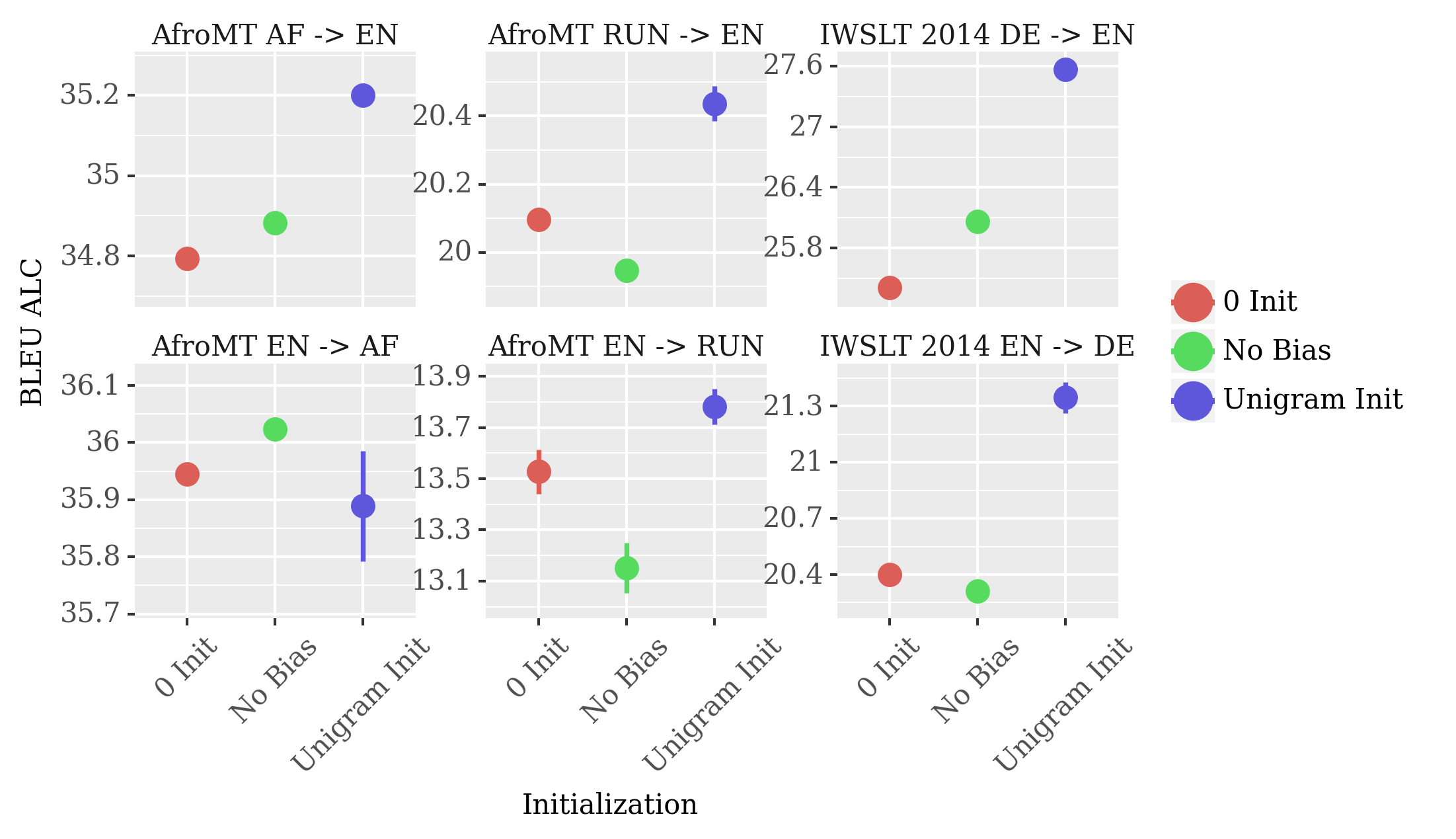
Figure 3: ALC of validation bleu for the first $20k$ training updates for each initialisation strategy. Models initialised with the unigram distribution achieve higher bleu earlier on in training, even when those models do not ultimately perform best (see Fig. 2).

Analysis.

The aim of this analysis is to investigate whether – and to what extent – the final-layer bias unigram initialisation leaves the contextual part of the network, $p_{\scaleto{\mathbf{W}\boldsymbol{\phi}}{4pt}}(\cdot\!\mid\!\mathbf{y}_{<t})$, to better capture non-frequency effects. To this end, we examine model-assigned log-probability as a function of token frequency. In Fig. 4, we plot a token’s unigram log-frequency against the average log-probability assigned to it (when it is the ground-truth token) by a model initialised with (left) a bias term of $\overset{\rightarrow}{0}$and (right) a log-unigram bias term, binning them in equal-length intervals and averaging them for clarity. In Fig. 4(a), the full model parameters are used. In Fig. 4(b), the bias terms are not added in the linear projection, i.e., only the contextual part of eq. 4, $p_{\scaleto{\mathbf{W}\boldsymbol{\phi}}{4pt}}(\cdot\!\mid\!\mathbf{y}_{<t})$, is computed.

The upward trend in average model-assigned log-probability in Fig. 4(a) suggests that, in general, models are better (or at least more confident) when predicting more frequent tokens. This trend holds when the bias term is omitted from the final linear computation of the $\overset{\rightarrow}{0}$-initialised model. Interestingly though, when the bias term is omitted from the unigram-initialised model, the trend appears to reverse. This change suggests that for unigram-initialised models, frequency may instead be encoded in the bias term, providing evidence that for these models, $p_{\scaleto{\mathbf{W}\boldsymbol{\phi}}{4pt}}(\cdot\!\mid\!\mathbf{y}_{<t})$ may indeed specialise in non-frequency aspects of language.

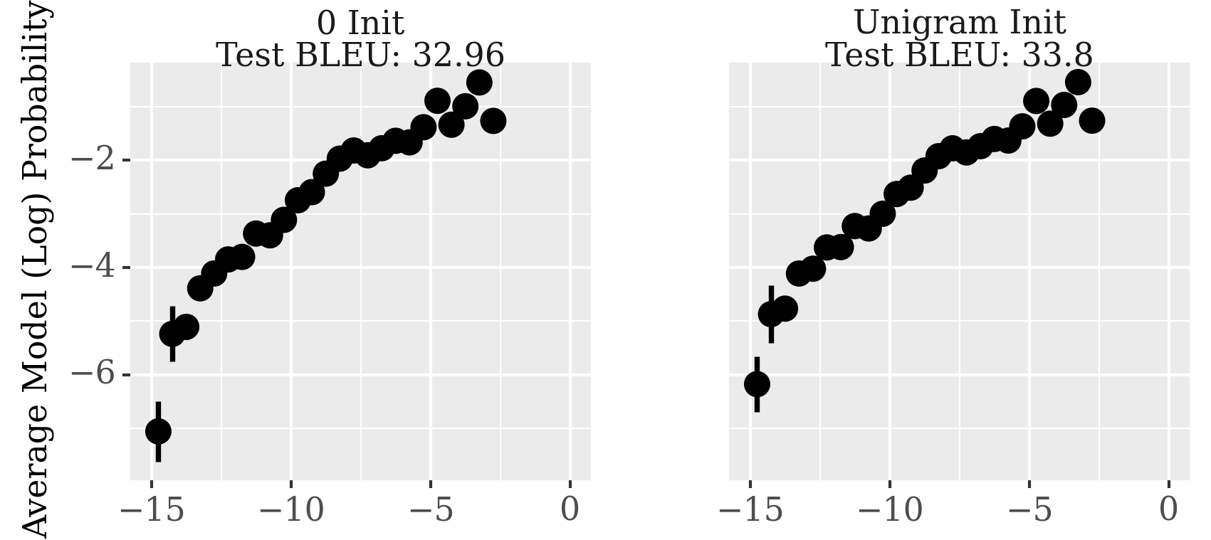
(a) Full model parameters used.

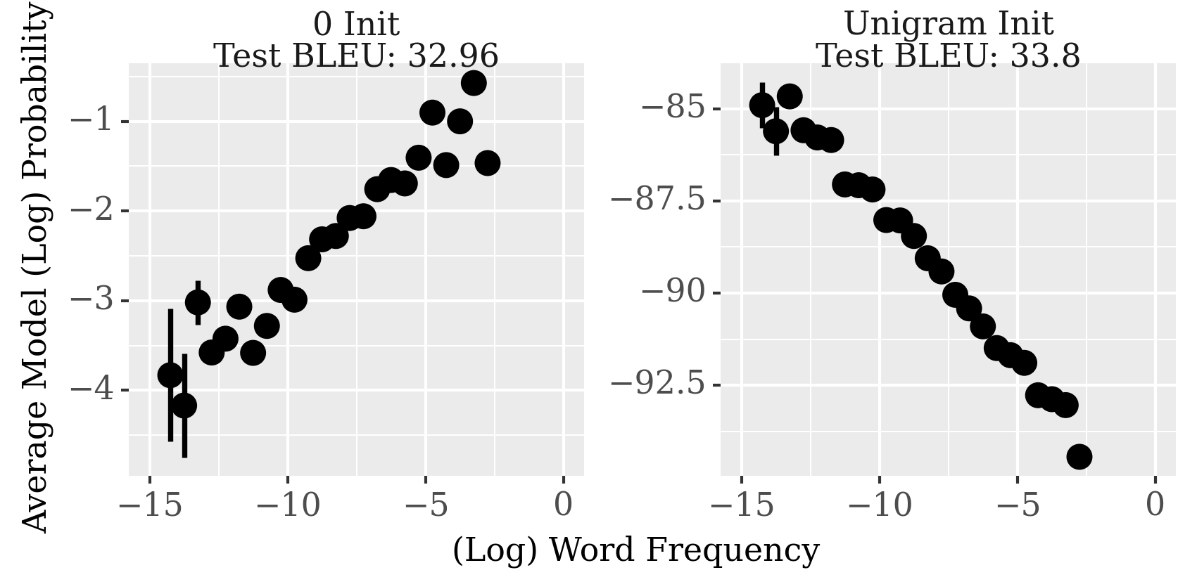
(b) Bias term removed.

Figure 4: Average log-probability assigned by the model to a ground-truth token in the test set vs. the log-unigram probability of that token in the training set (IWSLT’14 De$\rightarrow$En). Probabilities in upper row are computed using all model parameters; in the lower row, the bias term is dropped from the final linear projection.

5 Discussion

NLP models have been observed to overfit to surface cues in their training data, impeding their ability to generalise at inference time Warstadt et al. (2020); Wei et al. (2021). Thus, one could argue that learning or encoding the superficial statistical tendencies of language is not necessarily a good thing. Yet, empirical results suggest that it may in fact be an important part of model learning dynamics (see § A.4, for example). Indeed, Takahashi and Tanaka-Ishii (2019) find evidence that more powerful language models have a natural bias for learning them. Here we ask if – when initialising model parameters – we can explicitly endow our models with prior knowledge about one such statistical tendency: frequency.

While the result that this initialisation strategy improves training efficiency is perhaps not surprising, the relatively consistent improvement in overall performance is. We offer two possible explanations for this improvement. The first is that this initialisation beneficially alters model learning dynamics at the beginning of training, especially as early learning dynamics can have an outsized impact on final model performance Achille et al. (2019). A second possible explanation is that it disentangles frequency in the modelling of contextual probabilities. If $p_{b}$ (eq. 4) explicitly models the unigram distribution, then our model does not need to capture this component of the conditional distribution in its other parameters, which frees up model capacity to focus on more complex phenomena within natural language. Its success thus motivates exploring the use of higher-order statistical models, such as a bigram or trigram model, in an attempt to further disentangle surfaces statistics from more nuanced components of natural language in a modular fashion.

6 Conclusion and Future Work

In this work, we revisit a simple initialisation technique in the context of modern neural language generation models: setting the bias term in the final linear projection layer to the log-unigram distribution of (sub)words within the training corpus. This strategy leads to more efficient training; perhaps more surprisingly, it also leads to better overall performance in our machine translation experiments. We offer analysis and discussion as to the cause of these trends. An interesting direction for future work could be determining the effects that this initialisation procedure has on various model properties, e.g., its embedding space, and its benefits specifically in low-resource settings. Furthermore, extensions of this work could explore potential uses of this strategy in the mitigation of problems with lexically infrequent words, e.g., by analysing via the decomposition in eq. 4 whether a model’s probability estimate for a word is being driven by frequency or contextual components. Finally, this technique is not limited to models of distributions over strings; it is in fact applicable to any neural classification setting, the exploration of which is left to future work.

7 Acknowledgements

We would like to thank the members of the DeepMind Language Team for insightful discussions during the course of this work and specifically, Chris Dyer and Kris Cao for helpful feedback on the initial version of this paper and John Hale for pointers to references on human language acquisition. We would also like to thank Clément Guerner for detailed feedback on clarity and presentation.

8 Limitations

Perhaps the main limitation of this work is that we only explore the approach within the context of machine translation benchmarks, although we conduct extensive experiments within this task that cover different training data scales and diverse pairs of languages, including low-resource ones. Nevertheless, we remark that the proposed approach is entirely general-purpose, and can be applied to any other language generation or even any neural classification tasks. We leave it to future work to investigate whether the same gains would apply in those settings. Furthermore, we have not yet explored how this technique would interact with other modelling choices, such as different optimizers, training objectives, or subword tokenisation algorithms. Lastly, our unigram initialisation of the bias term is currently done at the level of subword units, which do not always correspond to lexically or morphologically meaningful linguistic units. We leave the extension of this approach to more meaningful linguistic units, such as words or morphemes, to future work.

9 Ethical Considerations

We foresee no ethical issues that could arise from the findings presented in this work.

Appendix A Additional Experiments

A.1 Additional Training Trends

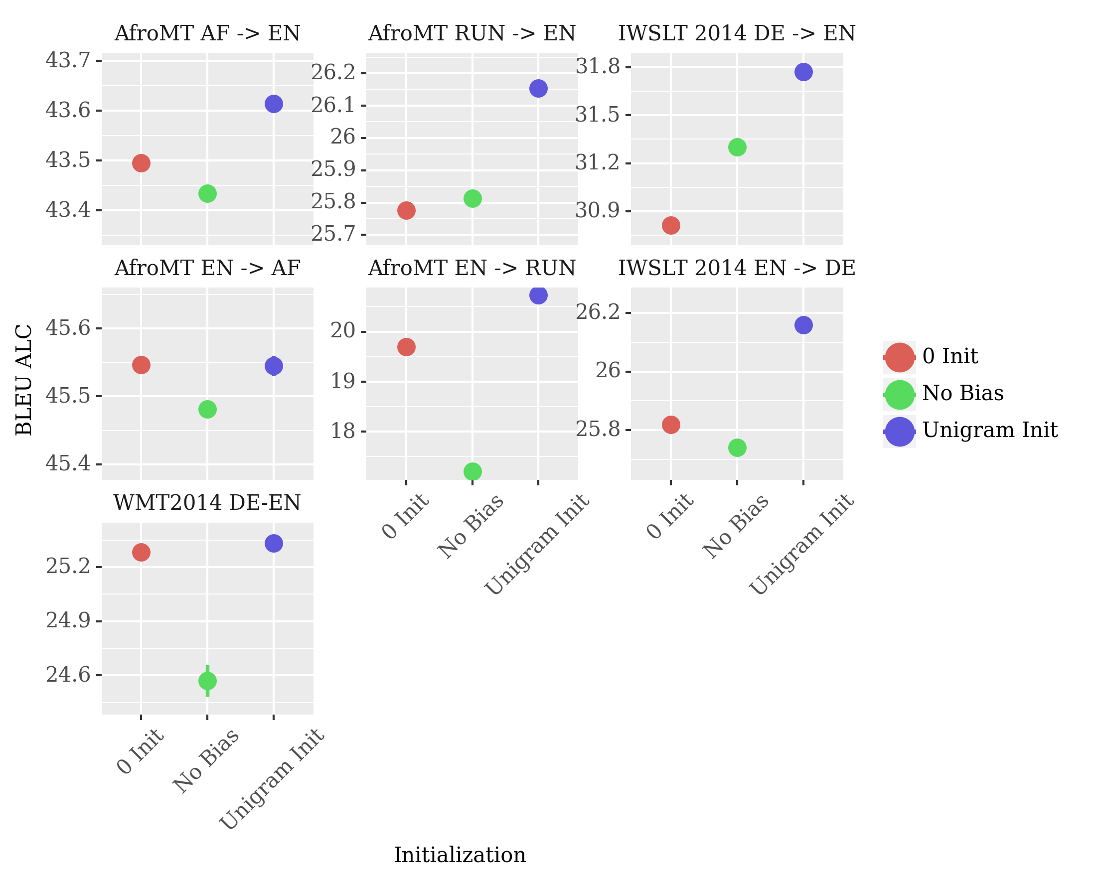
Figure 6: ALC scores for models over the full course of training. All other experimental details are the same as in Fig. 3.

A.2 WMT Experiments

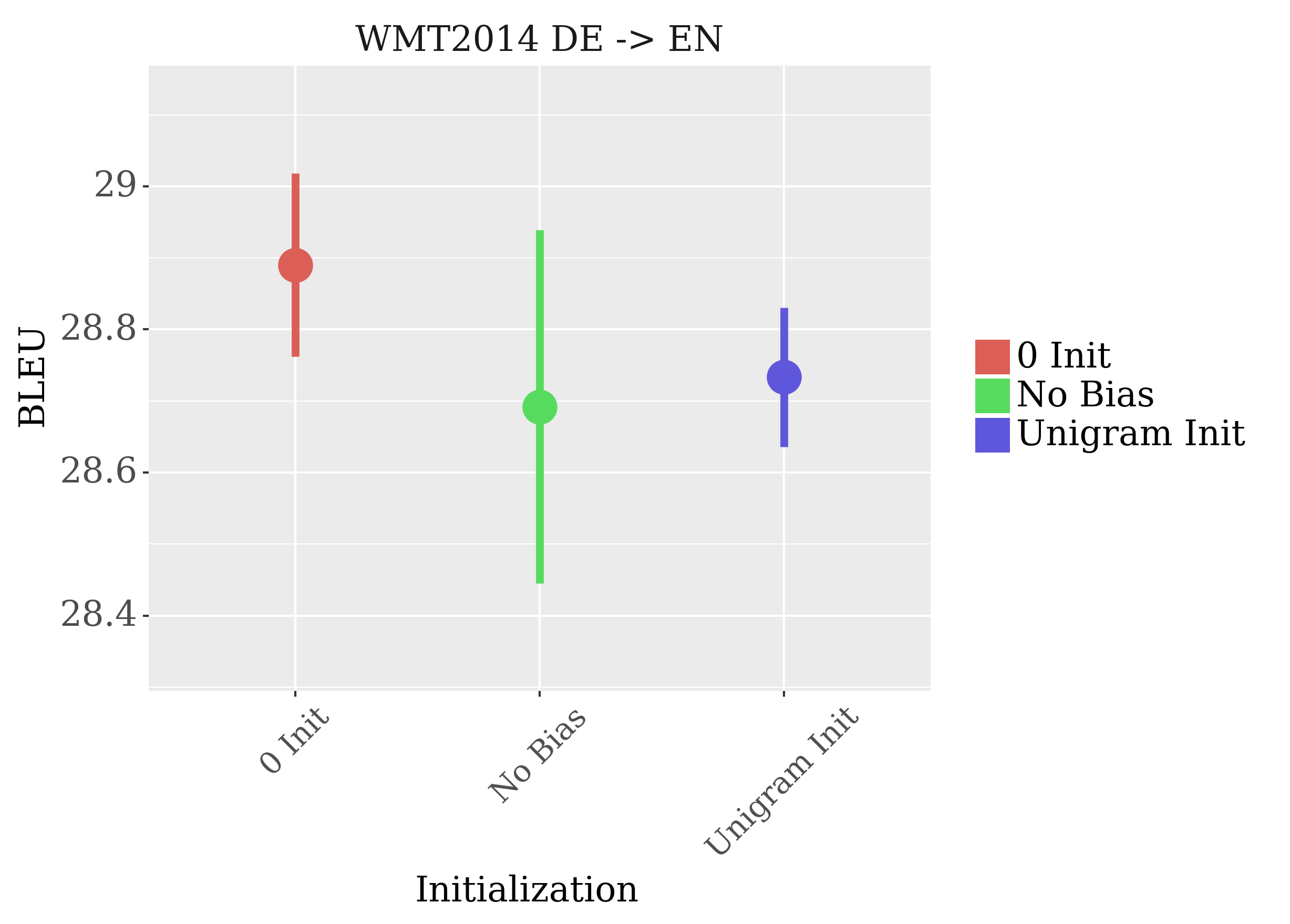
Figure 7: bleu scores on WMT’14 De$\rightarrow$En. Setup is the same as in Fig. 2.

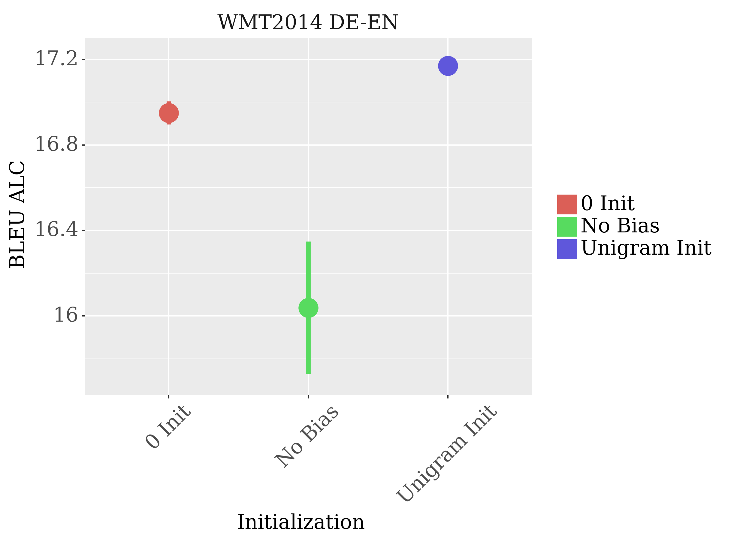
Figure 8: ALC scores on WMT’14 De$\rightarrow$En. Setup is the same as in Fig. 3.

A.3 chrF Scores

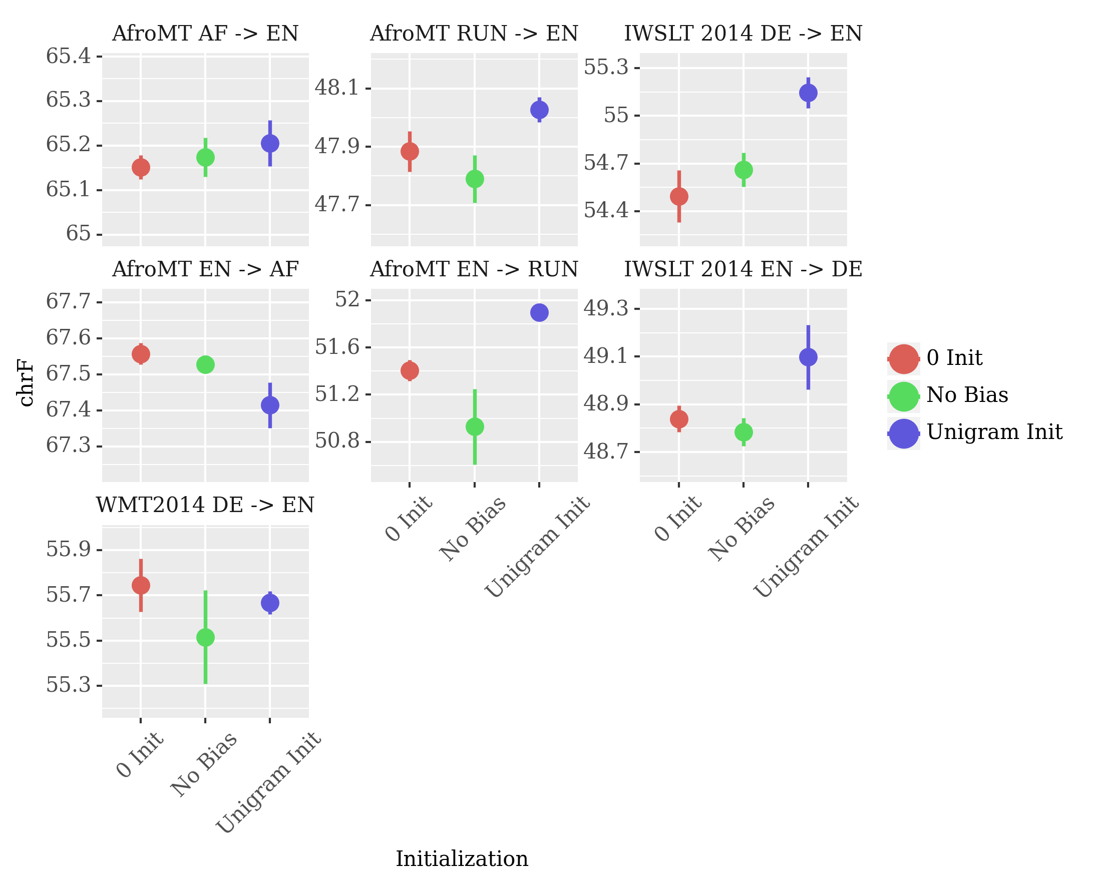
Figure 9: chrF scores on test set for models in Fig. 2. We observe the same trends.

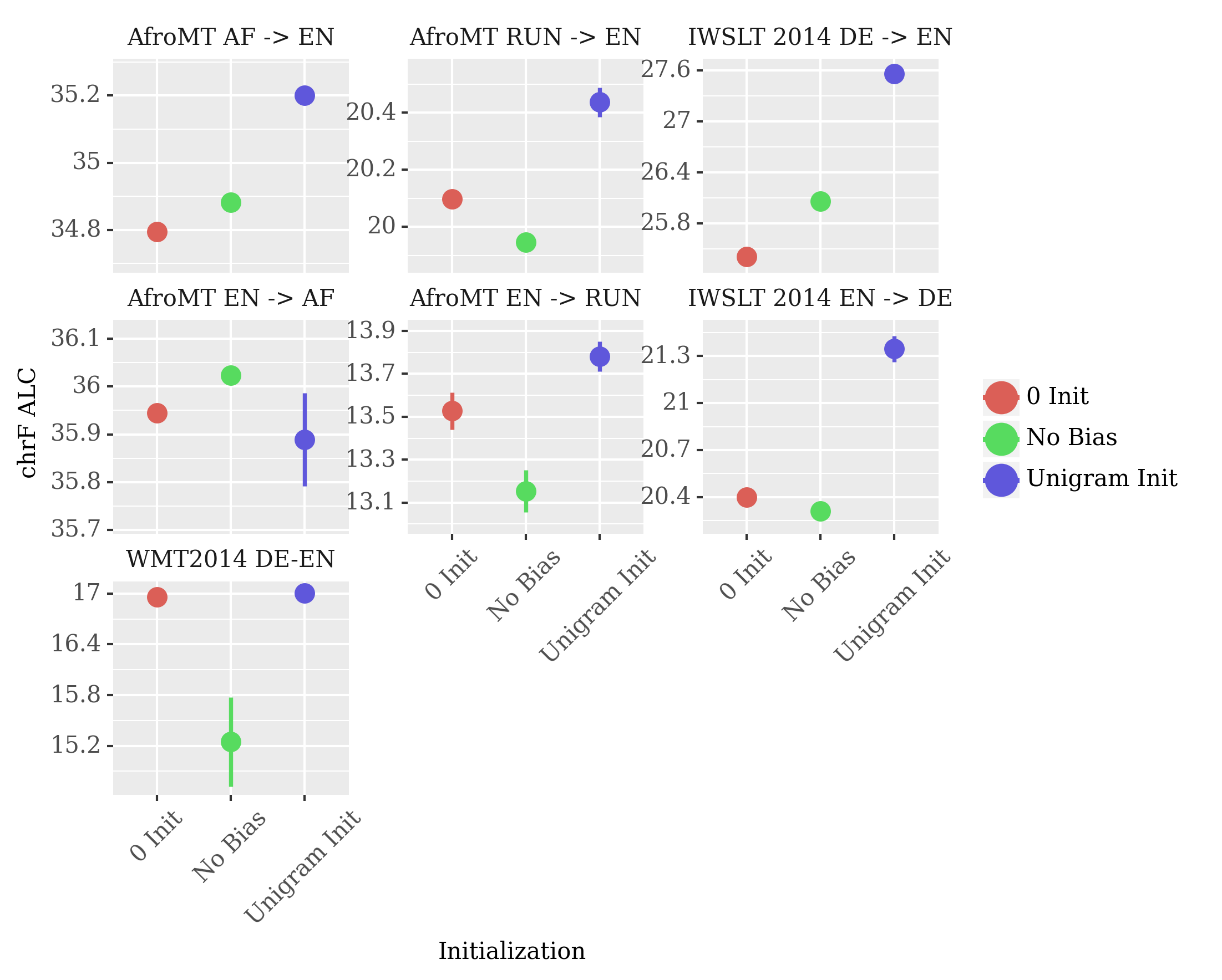
Figure 10: ALC scores using chrF as metric; again only the first $20$k steps are considered.

A.4 Regularising Away from the Unigram Distribution

Prior work has suggested that models’ learning of surface statistics, such as the unigram distribution, may harm their generalisation abilities Warstadt et al. (2020); Wei et al. (2021). Under this premise, it seems feasible that the learning trends observed in Fig. 1 could have downstream negative side-effects, e.g., the inappropriate preference for higher frequency words observed in Wei et al. (2021). Given the importance of early stage training dynamics Achille et al. (2019), it may even be the root cause of such behaviour. In the effort to test this hypothesis, we try to regularise a model’s output away from the unigram distribution in early stages of training. Specifically, we instead minimise the objective $\mathrm{KL}(p\mid\mid p_{\scaleto{{\boldsymbol{\theta}}}{4pt}})-\lambda\,\mathrm{KL}(\omega(p)\mid\mid p_{\scaleto{{\boldsymbol{\theta}}}{4pt}})$ for empirical distribution $p$ and the unigram distribution of this empirical distribution $\omega(p)$. $\lambda$ is a hyperparameter. We use this objective for the initial steps of training, then switching back to the standard objective $\mathrm{KL}(p\mid\mid p_{\scaleto{{\boldsymbol{\theta}}}{4pt}})$. In Fig. 11, we observe that this form of regularisation leads to worse (or equivalently performing) models by the time of convergence. Results were similar when evaluated on out-of-distribution data.

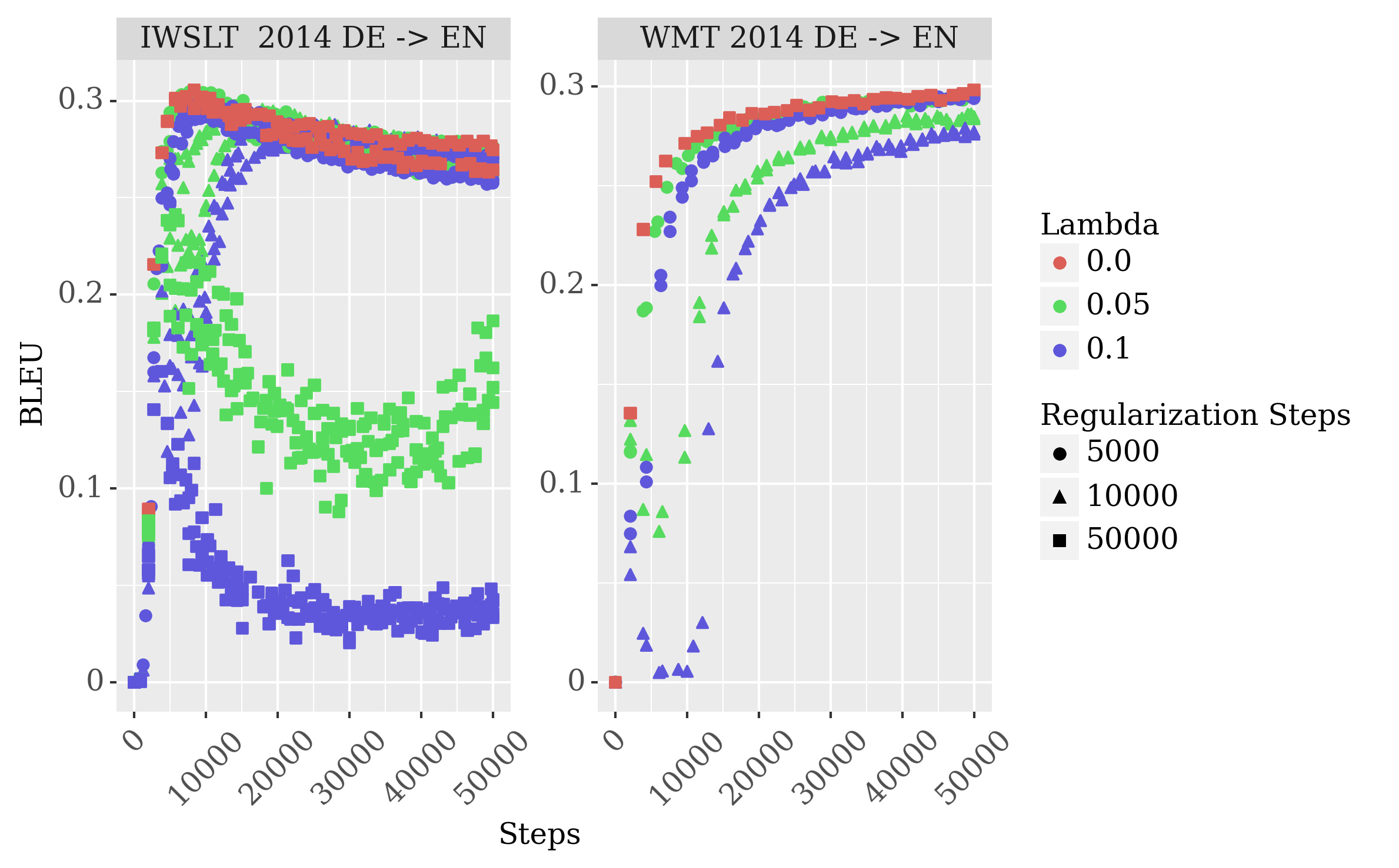
Figure 11: bleu scores (in decimal format) when regularising away from the unigram distribution. “Regularisation steps” indicates the point at which we change back to the standard objective.

A.5 Out-of-Domain Performance

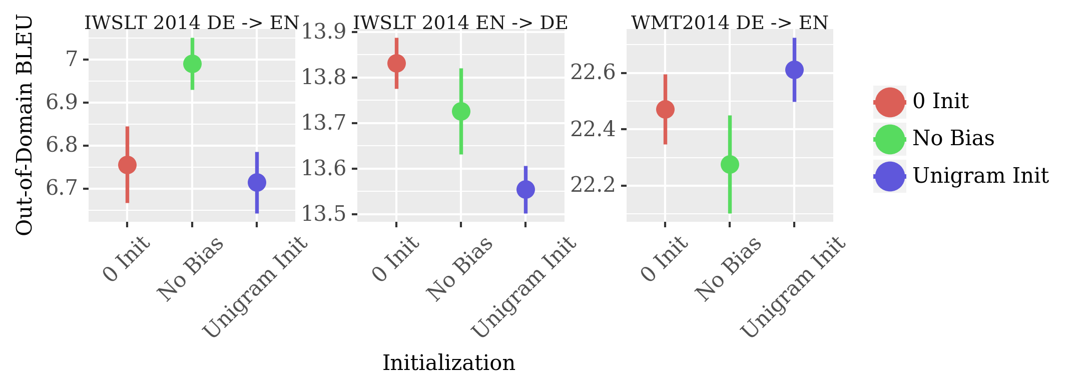
Figure 12: bleu on out-of-domain test sets (WMT14 for IWSLT and vice-versa) by bias initialisation strategies. Bars indicate standard error.

A.6 Change in Bias Term over Training

In Figs. 13 and 14, we see the divergence of the bias term from the unigram distribution and the magnitude of the bias term, respectively. Interestingly, we see that neither value changes perceptibly from the time of initialisation onward, suggesting the bias term itself does not change much from its initialised value. This trend is consistent across seeds and datasets.

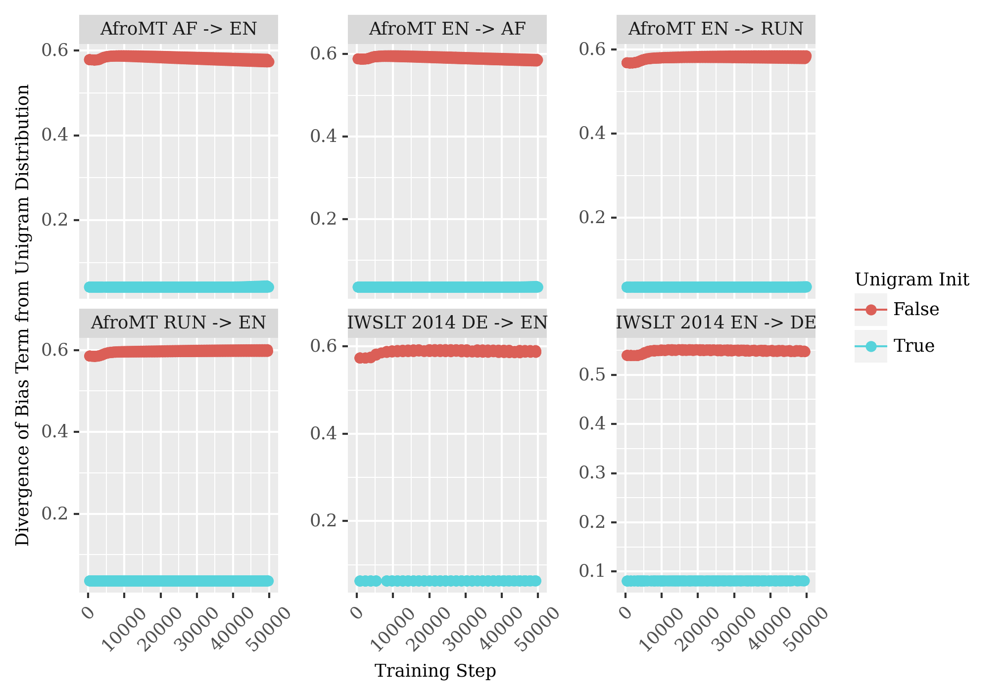
Figure 13: Divergence of the bias term (after $\mathrm{softmax}$ is performed to map bias onto probability simplex) from the unigram distribution of the respective training set for models trained on different data sets. Same models as used in Fig. 3.

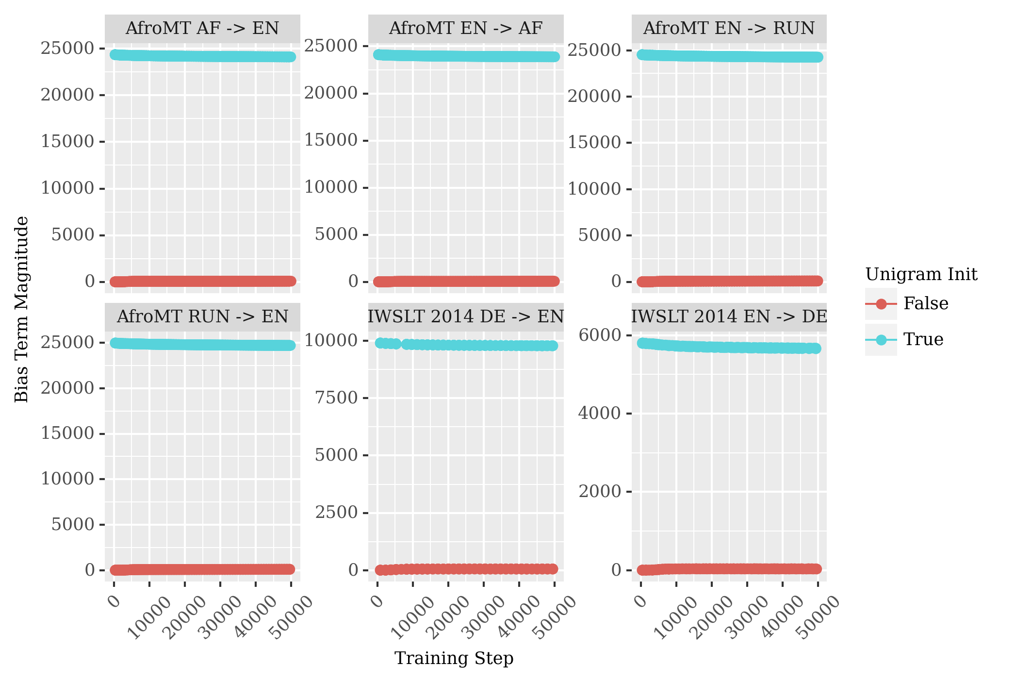
Figure 14: Magnitude of the bias term in models trained on different data sets. Same models as used in Fig. 3. Along with Fig. 13, these results suggest that the bias term does not change much from its value at parameter initialisation.

A.7 Initialisation with Bias Term from Large-Scale Dataset

We additionally explore the effects of initialising the bias term with the log-unigram distribution, as estimated from a larger dataset in a more general purpose domain. We hypothesise that this strategy could be useful in low resource settings. We find that this indeed improves the generalisation performance of a model trained on IWSLT when evaluated on an OOD dataset (see Fig. 16).

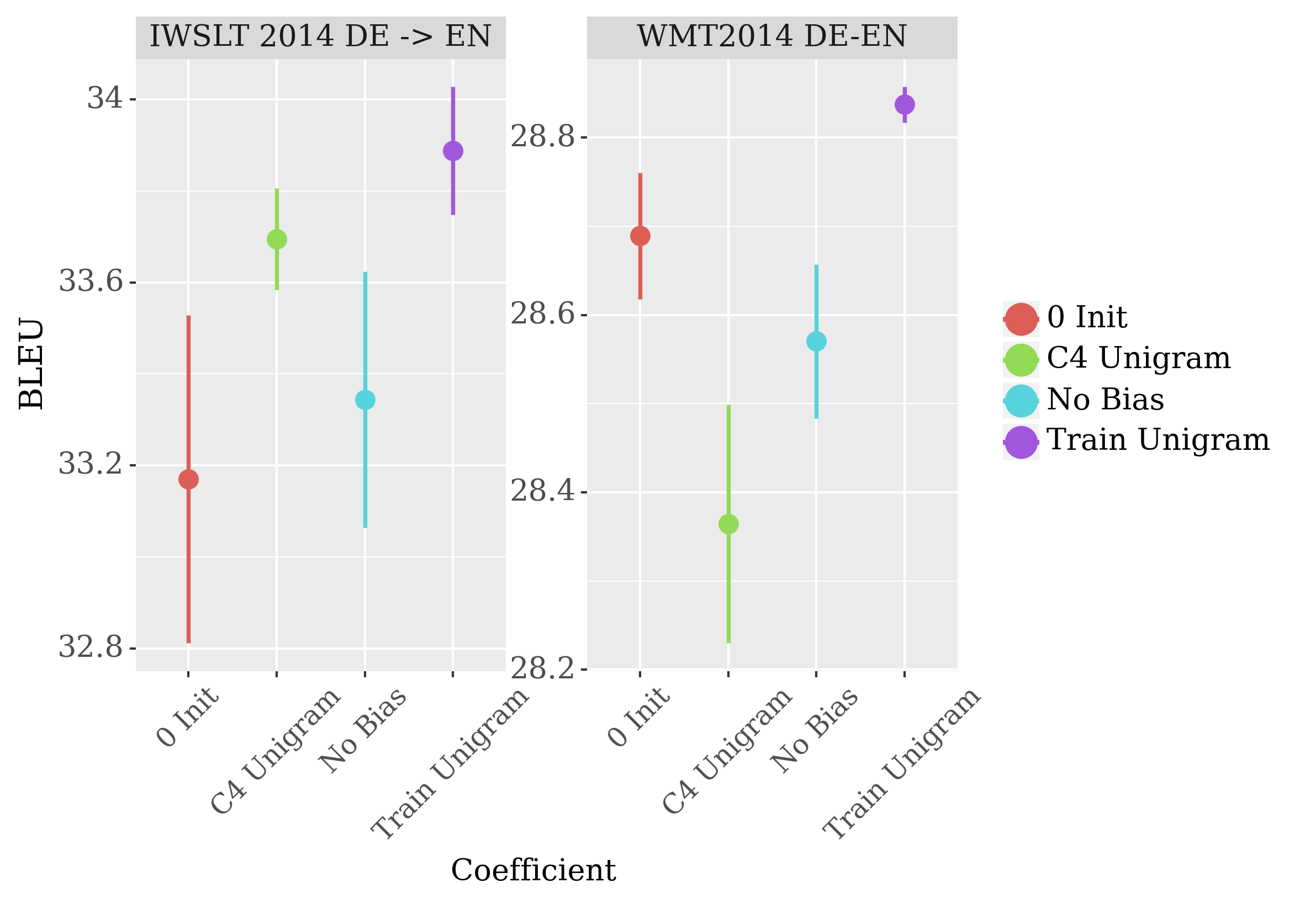
Figure 15: Results of best model checkpoint on validation set of respective datasets. Models are initialised with a $\overset{\rightarrow}{0}$bias term, no bias term, or the log-unigram distribution of either the C4 English dataset Raffel et al. (2019) or the respective training dataset.

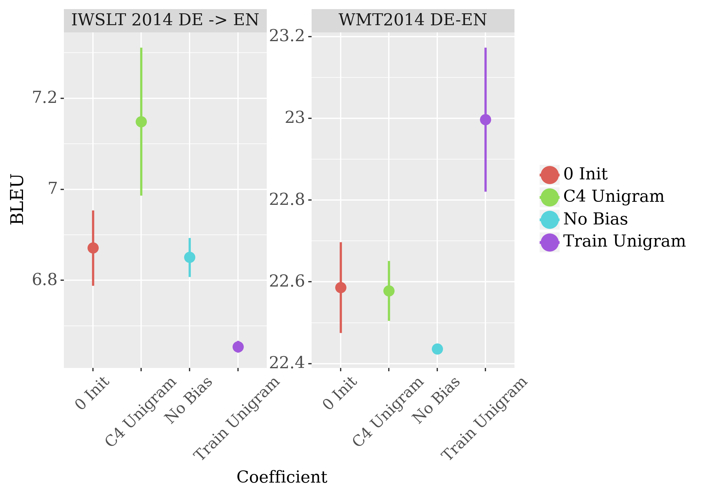
Figure 16: Results of best model checkpoint trained on IWSLT and WMT (as specified in facet label) and evaluated on (validation set of) out-of-domain datasets (WMT for the IWSLT model and vice-versa). Models are same as those in Fig. 15.

References

- Achille et al. (2019) Alessandro Achille, Matteo Rovere, and Stefano Soatto. 2019. Critical learning periods in deep networks. In 7th International Conference on Learning Representations.
- Adi et al. (2017) Yossi Adi, Einat Kermany, Yonatan Belinkov, Ofer Lavi, and Yoav Goldberg. 2017. Fine-grained analysis of sentence embeddings using auxiliary prediction tasks. In 5th International Conference on Learning Representations.
- Alain and Bengio (2017) Guillaume Alain and Yoshua Bengio. 2017. Understanding intermediate layers using linear classifier probes. In 5th International Conference on Learning Representations.
- Artetxe et al. (2022) Mikel Artetxe, Shruti Bhosale, Naman Goyal, Todor Mihaylov, Myle Ott, Sam Shleifer, Xi Victoria Lin, Jingfei Du, Srinivasan Iyer, Ramakanth Pasunuru, Giridharan Anantharaman, Xian Li, Shuohui Chen, Halil Akin, Mandeep Baines, Louis Martin, Xing Zhou, Punit Singh Koura, Brian O’Horo, Jeffrey Wang, Luke Zettlemoyer, Mona Diab, Zornitsa Kozareva, and Veselin Stoyanov. 2022. Efficient large scale language modeling with mixtures of experts. In Proceedings of the 2022 Conference on Empirical Methods in Natural Language Processing, pages 11699–11732, Abu Dhabi, United Arab Emirates. Association for Computational Linguistics.
- Baziotis et al. (2020) Christos Baziotis, Barry Haddow, and Alexandra Birch. 2020. Language model prior for low-resource neural machine translation. In Proceedings of the 2020 Conference on Empirical Methods in Natural Language Processing, pages 7622–7634, Online. Association for Computational Linguistics.
- Ben Zaken et al. (2022) Elad Ben Zaken, Yoav Goldberg, and Shauli Ravfogel. 2022. BitFit: Simple parameter-efficient fine-tuning for transformer-based masked language-models. In Proceedings of the 60th Annual Meeting of the Association for Computational Linguistics (Volume 2: Short Papers), pages 1–9, Dublin, Ireland. Association for Computational Linguistics.
- Berger and Printz (1998) Adam Berger and Harry Printz. 1998. A comparison of criteria for maximum entropy/ minimum divergence feature selection. In Proceedings of the Third Conference on Empirical Methods for Natural Language Processing, pages 96–106, Palacio de Exposiciones y Congresos, Granada, Spain. Association for Computational Linguistics.
- Bojar et al. (2014) Ondrej Bojar, Christian Buck, Christian Federmann, Barry Haddow, Philipp Koehn, Johannes Leveling, Christof Monz, Pavel Pecina, Matt Post, Herve Saint-Amand, Radu Soricut, Lucia Specia, and Aleš Tamchyna. 2014. Findings of the 2014 workshop on statistical machine translation. In Proceedings of the Ninth Workshop on Statistical Machine Translation, pages 12–58, Baltimore, Maryland, USA. Association for Computational Linguistics.
- Botha and Blunsom (2014) Jan Botha and Phil Blunsom. 2014. Compositional morphology for word representations and language modelling. In Proceedings of the 31st International Conference on Machine Learning, volume 32 of Proceedings of Machine Learning Research, pages 1899–1907, Bejing, China. PMLR.
- Cettolo et al. (2012) Mauro Cettolo, Christian Girardi, and Marcello Federico. 2012. WIT3: Web inventory of transcribed and translated talks. In Proceedings of the 16th Annual conference of the European Association for Machine Translation, pages 261–268, Trento, Italy. European Association for Machine Translation.
- Chang and Bergen (2022) Tyler A. Chang and Benjamin K. Bergen. 2022. Word acquisition in neural language models. Transactions of the Association for Computational Linguistics, 10:1–16.
- Chen and Goodman (1999) Stanley F. Chen and Joshua Goodman. 1999. An empirical study of smoothing techniques for language modeling. Computer Speech & Language, 13(4):359–394.
- Fang et al. (2015) Hao Fang, Mari Ostendorf, Peter Baumann, and Janet Pierrehumbert. 2015. Exponential language modeling using morphological features and multi-task learning. IEEE/ACM Transactions on Audio, Speech, and Language Processing, 23(12):2410–2421.
- Gerhand and Barry (1998) Simon Gerhand and Christopher Barry. 1998. Word frequency effects in oral reading are not merely age-of-acquisition effects in disguise. Journal of Experimental Psychology: Learning, Memory and Cognition, 24(4):267–83.
- Gilhooly and Logie (1980) Ken J Gilhooly and Robert H Logie. 1980. Age-of-acquisition, imagery, concreteness, familiarity, and ambiguity measures for 1,944 words. Behavior Research Methods & Instrumentation, 12(4):395–427.
- Glorot and Bengio (2010) Xavier Glorot and Yoshua Bengio. 2010. Understanding the difficulty of training deep feedforward neural networks. In Proceedings of the Thirteenth International Conference on Artificial Intelligence and Statistics, volume 9 of Proceedings of Machine Learning Research, pages 249–256, Chia Laguna Resort, Sardinia, Italy. PMLR.
- Grave et al. (2017) Edouard Grave, Armand Joulin, and Nicolas Usunier. 2017. Improving neural language models with a continuous cache. In 5th International Conference on Learning Representations.
- Guyon et al. (2011) Isabelle Guyon, Gavin C. Cawley, Gideon Dror, and Vincent Lemaire. 2011. Results of the active learning challenge. In Active Learning and Experimental Design workshop In conjunction with AISTATS 2010, volume 16 of Proceedings of Machine Learning Research, pages 19–45, Sardinia, Italy. PMLR.
- Hinton (2002) Geoffrey E. Hinton. 2002. Training products of experts by minimizing contrastive divergence. Neural Computation, 14(8):1771–1800.
- Kingma and Ba (2015) Diederik P. Kingma and Jimmy Ba. 2015. Adam: A method for stochastic optimization. In 3rd International Conference on Learning Representations.
- Kneser and Ney (1995) R. Kneser and H. Ney. 1995. Improved backing-off for M-gram language modeling. In 1995 International Conference on Acoustics, Speech, and Signal Processing, volume 1, pages 181–184 vol.1.
- Kudo and Richardson (2018) Taku Kudo and John Richardson. 2018. SentencePiece: A simple and language independent subword tokenizer and detokenizer for neural text processing. In Proceedings of the 2018 Conference on Empirical Methods in Natural Language Processing: System Demonstrations, pages 66–71, Brussels, Belgium. Association for Computational Linguistics.
- Le et al. (2015) Quoc V. Le, Navdeep Jaitly, and Geoffrey E. Hinton. 2015. A simple way to initialize recurrent networks of rectified linear units. CoRR, abs/1504.00941.
- Li et al. (2022) Huayang Li, Deng Cai, Jin Xu, and Taro Watanabe. 2022. -gram is back: Residual learning of neural text generation with -gram language model. In Proceedings of the 2022 Conference on Empirical Methods in Natural Language Processing, Abu Dhabi, United Arab Emirates. Association for Computational Linguistics.
- Liu et al. (2021) Zeyu Liu, Yizhong Wang, Jungo Kasai, Hannaneh Hajishirzi, and Noah A. Smith. 2021. Probing across time: What does RoBERTa know and when? In Findings of the Association for Computational Linguistics: EMNLP 2021, pages 820–842, Punta Cana, Dominican Republic. Association for Computational Linguistics.
- Liu et al. (2020) Zhengying Liu, Zhen Xu, Shangeth Rajaa, Meysam Madadi, Julio C. S. Jacques Junior, Sergio Escalera, Adrien Pavao, Sebastien Treguer, Wei-Wei Tu, and Isabelle Guyon. 2020. Towards automated deep learning: Analysis of the AutoDL challenge series 2019. In Proceedings of the NeurIPS 2019 Competition and Demonstration Track, volume 123 of Proceedings of Machine Learning Research, pages 242–252. PMLR.
- Meister and Cotterell (2021) Clara Meister and Ryan Cotterell. 2021. Language model evaluation beyond perplexity. In Proceedings of the 59th Annual Meeting of the Association for Computational Linguistics and the 10th International Joint Conference on Natural Language Processing (Volume 1: Long Papers), pages 5328–5339, Online. Association for Computational Linguistics.
- Mnih and Hinton (2007) Andriy Mnih and Geoffrey Hinton. 2007. Three new graphical models for statistical language modelling. In Proceedings of the 24th International Conference on Machine Learning, ICML ’07, page 641–648, New York, NY, USA. Association for Computing Machinery.
- Morrison et al. (1997) Catriona M. Morrison, Tameron D. Chappell, and Andrew W. Ellis. 1997. Age of acquisition norms for a large set of object names and their relation to adult estimates and other variables. The Quarterly Journal of Experimental Psychology Section A, 50(3):528–559.
- Morton (1969) John Morton. 1969. Interaction of information in word recognition. Psychological Review, 76(2):165.
- Mu et al. (2018) Norman Mu, Zhewei Yao, Amir Gholami, Kurt Keutzer, and Michael W. Mahoney. 2018. Parameter re-initialization through cyclical batch size schedules. CoRR, abs/1812.01216.
- Neubig and Dyer (2016) Graham Neubig and Chris Dyer. 2016. Generalizing and hybridizing count-based and neural language models. In Proceedings of the 2016 Conference on Empirical Methods in Natural Language Processing, pages 1163–1172, Austin, Texas. Association for Computational Linguistics.
- Nikkarinen et al. (2021) Irene Nikkarinen, Tiago Pimentel, Damián Blasi, and Ryan Cotterell. 2021. Modeling the unigram distribution. In Findings of the Association for Computational Linguistics: ACL-IJCNLP 2021, pages 3721–3729. Association for Computational Linguistics.
- Papineni et al. (2002) Kishore Papineni, Salim Roukos, Todd Ward, and Wei-Jing Zhu. 2002. BLEU: A method for automatic evaluation of machine translation. In Proceedings of the 40th Annual Meeting of the Association for Computational Linguistics, pages 311–318, Philadelphia, Pennsylvania, USA. Association for Computational Linguistics.
- Popović (2015) Maja Popović. 2015. chrF: Character n-gram F-score for automatic MT evaluation. In Proceedings of the Tenth Workshop on Statistical Machine Translation, pages 392–395, Lisbon, Portugal. Association for Computational Linguistics.
- Post (2018) Matt Post. 2018. A call for clarity in reporting BLEU scores. In Proceedings of the Third Conference on Machine Translation: Research Papers, pages 186–191, Belgium, Brussels. Association for Computational Linguistics.
- Puccetti et al. (2022) Giovanni Puccetti, Anna Rogers, Aleksandr Drozd, and Felice Dell’Orletta. 2022. Outlier dimensions that disrupt transformers are driven by frequency. In Findings of the Association for Computational Linguistics: EMNLP 2022, pages 1286–1304, Abu Dhabi, United Arab Emirates. Association for Computational Linguistics.
- Raffel et al. (2019) Colin Raffel, Noam Shazeer, Adam Roberts, Katherine Lee, Sharan Narang, Michael Matena, Yanqi Zhou, Wei Li, and Peter J. Liu. 2019. Exploring the limits of transfer learning with a unified text-to-text transformer. CoRR, abs/1910.10683.
- Rajaee and Pilehvar (2022) Sara Rajaee and Mohammad Taher Pilehvar. 2022. An isotropy analysis in the multilingual BERT embedding space. In Findings of the Association for Computational Linguistics: ACL 2022, pages 1309–1316, Dublin, Ireland. Association for Computational Linguistics.
- Reid et al. (2021) Machel Reid, Junjie Hu, Graham Neubig, and Yutaka Matsuo. 2021. AfroMT: Pretraining strategies and reproducible benchmarks for translation of 8 african languages. In Proceedings of the 2021 Conference on Empirical Methods in Natural Language Processing, Punta Cana, Dominican Republic.
- Szegedy et al. (2015) Christian Szegedy, Vincent Vanhoucke, Sergey Ioffe, Jon Shlens, and Zbigniew Wojna. 2015. Rethinking the inception architecture for computer vision. 2016 IEEE Conference on Computer Vision and Pattern Recognition, pages 2818–2826.
- Takahashi and Tanaka-Ishii (2017) Shuntaro Takahashi and Kumiko Tanaka-Ishii. 2017. Do neural nets learn statistical laws behind natural language? PLOS ONE, 12(12):1–17.
- Takahashi and Tanaka-Ishii (2019) Shuntaro Takahashi and Kumiko Tanaka-Ishii. 2019. Evaluating computational language models with scaling properties of natural language. Transactions of the Association for Computational Linguistics, 45(3):481–513.
- Teh (2006) Yee Whye Teh. 2006. A hierarchical Bayesian language model based on Pitman-Yor processes. In Proceedings of the 21st International Conference on Computational Linguistics and 44th Annual Meeting of the Association for Computational Linguistics, pages 985–992, Sydney, Australia. Association for Computational Linguistics.
- Vaswani et al. (2017) Ashish Vaswani, Noam Shazeer, Niki Parmar, Jakob Uszkoreit, Llion Jones, Aidan N. Gomez, Łukasz Kaiser, and Illia Polosukhin. 2017. Attention is all you need. In Advances in Neural Information Processing Systems 30, pages 5998–6008.
- Warstadt et al. (2020) Alex Warstadt, Yian Zhang, Xiaocheng Li, Haokun Liu, and Samuel R. Bowman. 2020. Learning which features matter: RoBERTa acquires a preference for linguistic generalizations (eventually). In Proceedings of the 2020 Conference on Empirical Methods in Natural Language Processing, pages 217–235, Online. Association for Computational Linguistics.
- Wei et al. (2021) Jason Wei, Dan Garrette, Tal Linzen, and Ellie Pavlick. 2021. Frequency effects on syntactic rule learning in transformers. In Proceedings of the 2021 Conference on Empirical Methods in Natural Language Processing, pages 932–948, Online and Punta Cana, Dominican Republic. Association for Computational Linguistics.
- Zevin and Seidenberg (2002) Jason D. Zevin and Mark S. Seidenberg. 2002. Age of acquisition effects in word reading and other tasks. Journal of Memory and Language, 47(1):1–29.