C i and CO in Nearby Spiral Galaxies - I. Line Ratio and Abundance Variations at $\sim 200$ pc Scales

We present new neutral atomic carbon [C i] (${}^{3}P_{1}\leavevmode\nobreak\ \to\leavevmode\nobreak\ {}^{3}P_{0}$) mapping observations within the inner $\sim 7$ kpc and $\sim 4$ kpc of the disks of NGC 3627 and NGC 4321 at a spatial resolution of 190 pc and 270 pc, respectively, using the Atacama Large Millimeter/Submillimeter Array (ALMA) Atacama Compact Array (ACA). We combine these with the CO(2–1) data from PHANGS-ALMA, and literature [C i] and CO data for two other starburst and/or active galactic nucleus (AGN) galaxies (NGC 1808, NGC 7469), to study: a) the spatial distributions of C i and CO emission; b) the observed line ratio $R_{{\mathrm{C\text{\sc{i}}}}/{\mathrm{CO}}}=I_{\mathrm{[C{\textsc{i}}]}(1\textnormal{--}0)}/I_{\mathrm{CO}(2\textnormal{--}1)}$ as a function of various galactic properties; and c) the abundance ratio of [C i/CO]. We find excellent spatial correspondence between C i and CO emission and nearly uniform $R_{{\mathrm{C\text{\sc{i}}}}/{\mathrm{CO}}}\sim 0.1$ across the majority of the star-forming disks of NGC 3627 and NGC 4321. However, $R_{{\mathrm{C\text{\sc{i}}}}/{\mathrm{CO}}}$ strongly varies from $\sim 0.05$ at the centre of NGC 4321 to $>0.2\text{--}0.5$ in NGC 1808’s starbursting centre and NGC 7469’s centre with an X-ray-luminous active galactic nucleus (AGN). Meanwhile, $R_{{\mathrm{C\text{\sc{i}}}}/{\mathrm{CO}}}{}$ does not obviously vary with $\left<U\right>$, similar to the prediction of photodissociation dominated region (PDR) models. We also find a mildly decreasing $R_{{\mathrm{C\text{\sc{i}}}}/{\mathrm{CO}}}{}$ with an increasing metallicity over $0.7\text{--}0.85\,\mathrm{Z_{\odot}}$, consistent with the literature. Assuming various typical ISM conditions representing giant molecular clouds, active star-forming regions and strong starbursting environments, we calculate the local-thermodynamic-equilibrium radiative transfer and estimate the [C i/CO] abundance ratio to be $\sim 0.1$ across the disks of NGC 3627 and NGC 4321, similar to previous large-scale findings in Galactic studies. However, this abundance ratio likely has a substantial increase to $\sim 1$ and $\gtrsim 1$–5 in NGC 1808’s starburst and NGC 7469’s strong AGN environments, respectively, in line with the expectations for cosmic-ray dominated region (CRDR) and X-ray dominated region (XDR) chemistry. Finally, we do not find a robust evidence for a generally CO-dark, C i-bright gas in the disk areas we probed.

1 Introduction

1.1 Neutral atomic carbon in the interstellar medium

Neutral atomic carbon (C⁰ or C i) is an important phase of carbon in the interstellar medium (ISM) besides ionized carbon (C⁺ or C ii) and carbon monoxide (CO). Its ${}^{3}P$ state is split into three fine-structure levels. The ${}^{3}P_{1}\to{}^{3}P_{0}$ transition line at 492.16065 GHz, hereafter $[\mathrm{C}\,{\text{\sc{i}}}]\,(1\textnormal{--}0)$, has an upper energy level of $E_{u}=23.620$ K and a critical density of $n_{\mathrm{crit}}\sim 1.0\times 10^{3}\;\mathrm{cm^{-3}}$ (at a temperature of 50 K) , and the ${}^{3}P_{2}\to{}^{3}P_{1}$ transition line at 809.34197 GHz has $E_{u}=62.462$ K and $n_{\mathrm{crit}}\sim 3.4\times 10^{3}\;\mathrm{cm^{-3}}$. Therefore, they are easily excited in the cold ISM environment. Given the high abundance of carbon in the ISM, C i, CO and C ii are the most powerful cold ISM tracers, and are the most widely used tools to probe cold ISM properties and hence galaxy evolution at cosmological distances.

The interstellar C i is produced from the photodissociation of CO molecules by UV photons and the recombination of C ii, both happening in photodissociation regions (PDRs; Langer 1976; de Jong et al. 1980; Tielens & Hollenbach 1985a, b; van Dishoeck & Black 1986, 1988; Sternberg & Dalgarno 1989, 1995; Hollenbach et al. 1991; Hollenbach & Tielens 1999; Kaufman et al. 1999; Wolfire et al. 2010; Madden et al. 2020; Bisbas et al. 2021, also see reviews by Genzel & Stutzki 1989; Jaffe et al. 1985; Hollenbach & Tielens 1997; Wolfire et al. 2022). In the simple plane-parallel (i.e., 1-D) PDR model, C i exists in a layer where UV photons can penetrate through the molecular gas but cannot maintain a high carbon ionizing rate. Such a layer is suggested to have an intermediate gas surface density ($N_{\mathrm{H_{2}}}\sim 1\textnormal{--}4\times 10^{20}\;\mathrm{cm^{-2}}$), fairly cold temperature (10 to a few tens K), and moderate visual extinction ($A_{V}\sim 1-4$). CO molecules dominate the more shielded interior of this layer and C ii dominates the exterior. Hydrogen molecules are gradually photodissociated to atoms across this layer ($A_{V}\sim 0.1-4$). This plane-parallel scenario qualitatively explains the layered structure of the Orion Bar PDR in our Galaxy on sub-pc scales (e.g., Genzel & Stutzki 1989; Tielens et al. 1993; Tauber et al. 1994; Hogerheijde et al. 1995; Hollenbach & Tielens 1999; Goicoechea et al. 2016), and the $\rho$ Ophiuchi A PDR in a recent study with an unprecedented resolution of 360 AU (Yamagishi et al. 2021), where the interplay between individual young, massive (O, B) stars and the ISM can be directly observed.

However, such simple models cannot fully explain molecular clouds. Plenty of observations in Galactic molecular clouds, H ii regions and star-formation complexes have revealed a widespread C i distribution over most areas of molecular clouds on scales of a few to ten pc, and a relatively high C i fractional abundance even at a large $A_{V}$ depth $>10$ mag (Phillips et al. 1980; Phillips & Huggins 1981; Wootten et al. 1982; Keene et al. 1985, 1987; Jaffe et al. 1985; Zmuidzinas et al. 1986, 1988; Genzel et al. 1988; Frerking et al. 1989; Plume et al. 1994, 1999; Gerin et al. 1998; Tatematsu et al. 1999; Ikeda et al. 1999, 2002; Yamamoto et al. 2001; Zhang et al. 2001; Kamegai et al. 2003; Oka et al. 2004; Izumi et al. 2021).

This observational evidence actually requires PDRs to be clumpy (Stutzki et al. 1988; Genzel et al. 1988; Burton et al. 1990; Meixner & Tielens 1993; Spaans & van Dishoeck 1997; Kramer et al. 2004, 2008; Pineda et al. 2008; Sun et al. 2008), with a volume filling factor much less than unity (e.g., $\sim 0.1-0.3$; Stutzki et al. 1988), so that UV photons can penetrate through most of the cloud, except for the densest clumps. Therefore, the spatial co-existence of C i and low rotational transition (low-$J$) CO lines can be well explained by such an inter-clump medium inside the molecular clouds. Alternatively, cosmic rays (CRs) have also been proposed to be the reason for the C i-CO association as they can penetrate much deeper than UV photons into clouds, and thus more uniformly dissociate CO molecules into C i inside clouds (Field et al. 1969; Padovani et al. 2009; Papadopoulos 2010; Ivlev et al. 2015; Papadopoulos et al. 2018).

1.2 Variations of the C i/CO line ratio ($R_{{\mathrm{C\text{\sc{i}}}}/{\mathrm{CO}}}$) in the literature

Although the spatial distributions of C i and low-$J$ CO emission resemble each other surprisingly well from molecular clouds to Galactic scales (e.g., across the Galactic plane; Wright et al. 1991; Bennett et al. 1994; Oka et al. 2005; Burton et al. 2015) and in external galaxies with spatially resolved observations (e.g., Schilke et al. 1993; White et al. 1994; Harrison et al. 1995; Israel et al. 1995; Israel & Baas 2001, 2003; Zhang et al. 2014; Krips et al. 2016; Cicone et al. 2018; Crocker et al. 2019; Jiao et al. 2019; Miyamoto et al. 2018, 2021; Salak et al. 2019; Izumi et al. 2020; Saito et al. 2020; Michiyama et al. 2020, 2021), their line intensity ratio, ${R}_{\mathrm{C{\text{\sc{i}}}{10}}/\mathrm{CO{10}}}=I_{[\mathrm{C}\,{\text{\sc{i}}}]\,(1\textnormal{--}0)}/I_{\mathrm{CO}\,(1\textnormal{--}0)}$ , does vary according to local ISM conditions — C i and CO fractional abundance (i.e., metallicity), excitation condition (e.g., excitation temperature $T_{\mathrm{ex}}$ and optical depth $\tau$), and UV and/or CR radiation field. At individual molecular cloud scales, ${R}_{\mathrm{C{\text{\sc{i}}}{10}}/\mathrm{CO{10}}}$ (or column density ratio) seems to vary from $\gtrsim 0.5$ (or $\gtrsim 0.2$ for column density ratio) to $<0.1$ with an increasing $N_{\mathrm{H2}}$ and $A_{V}$, e.g., from cloud surface or PDR front to the interior (e.g. Frerking et al. 1982; Genzel et al. 1988; Oka et al. 2004; Kramer et al. 2004, 2008; Mookerjea et al. 2006; Sun et al. 2008; Yamagishi et al. 2021).

At sub-galactic scales, when individual clouds are smoothed out, ${R}_{\mathrm{C{\text{\sc{i}}}{10}}/\mathrm{CO{10}}}$ is found to lie in a narrower range of $\sim 0.1\text{--}0.3$. For example, across the Galactic plane, the ratio is found to change only slightly within a galactocentric radius of 3–7 kpc ($\sim 0.08\text{--}0.12$, overall mean $=0.105\pm 0.004$; Oka et al. 2005); whereas in the starburst galaxies like M 82 and NGC 253, ${R}_{\mathrm{C{\text{\sc{i}}}{10}}/\mathrm{CO{10}}}$ or the [C i]/CO abundance ratio is a factor of 3–5 higher than the Galactic value (Schilke et al. 1993; White et al. 1994; Krips et al. 2016). Recent high-resolution (hundred pc scales) $[\mathrm{C}\,{\text{\sc{i}}}]\,(1\textnormal{--}0)$ mapping studies in the nearby spiral galaxy M 83 (Miyamoto et al. 2021) and starburst galaxy IRAS F18293-3413 (Saito et al. 2020) reported tightly-correlated $[\mathrm{C}\,{\text{\sc{i}}}]\,(1\textnormal{--}0)$ and $\mathrm{CO}\,(1\textnormal{--}0)$ emission, with scaling relations at hundred parsecs equivalent to ${R}_{\mathrm{C{\text{\sc{i}}}{10}}/\mathrm{CO{10}}}=0.14\times(L^{\prime}_{\mathrm{CO}\,(1\textnormal{--}0)}/10^{6.0}\,[\mathrm{K\,km\,s^{-1}\,pc^{2}}])^{-0.13}$ and ${R}_{\mathrm{C{\text{\sc{i}}}{10}}/\mathrm{CO{10}}}=0.21\times(L^{\prime}_{\mathrm{CO}\,(1\textnormal{--}0)}/10^{6.8}\,[\mathrm{K\,km\,s^{-1}\,pc^{2}}])^{+0.54}$, respectively. The discrepant power-law indices reflects different trends in individual galaxies that are not fully understood.

Meanwhile, in the central $\lesssim 100$ pc of NGC 7469 close to the X-ray-luminous active galactic nucleus (AGN), $R_{{\mathrm{C\text{\sc{i}}}}/{\mathrm{CO}}}$ is found to be substantially enhanced by a factor of $>10$ (reaching ${R}_{\mathrm{C{\text{\sc{i}}}{10}}/\mathrm{CO{10}}}\approx 1$; Izumi et al. 2020; see also the Circinus Galaxy’s AGN with ${R}_{\mathrm{C{\text{\sc{i}}}{10}}/\mathrm{CO{32}}}\approx 0.9$ in Izumi et al. 2018).

Furthermore, in the low-metallicity Large Magellanic Cloud (LMC) and Small Magellanic Cloud (SMC) environments, a factor of $1.5-3\times$ higher $R_{{\mathrm{C\text{\sc{i}}}}/{\mathrm{CO}}}$ values have been found (Bolatto et al. 2000b, a; see also other low-metallicity galaxies: Bolatto et al. 2000c; Hunt et al. 2017).

These studies indicate that $R_{{\mathrm{C\text{\sc{i}}}}/{\mathrm{CO}}}$ is sensitive to ISM conditions among and within galaxies. However, previous extragalactic studies are mainly focused on starburst galaxies and bright galaxy centres. How $R_{{\mathrm{C\text{\sc{i}}}}/{\mathrm{CO}}}$ behaves across the disks and spiral arms of typical star-forming galaxies is much less explored. Whether C i can trace the so-called CO-dark molecular gas at a low gas density or metallicity is also still in question. Understanding $R_{{\mathrm{C\text{\sc{i}}}}/{\mathrm{CO}}}$ variation and quantifying the C i and CO excitation in extragalactic environments is now particularly important given the rapidly growing numbers and diverse galactic environments of C i line observations at cosmological distances (e.g., Weiß et al. 2003, 2005; Pety et al. 2004; Wagg et al. 2006; Walter et al. 2011; Danielson et al. 2011; Alaghband-Zadeh et al. 2013; Gullberg et al. 2016; Bothwell et al. 2017; Popping et al. 2017; Yang et al. 2017; Emonts et al. 2018; Valentino et al. 2018, 2020; Bourne et al. 2019; Nesvadba et al. 2019; Dannerbauer et al. 2019; Jin et al. 2019; Brisbin et al. 2019; Boogaard et al. 2020; Cortzen et al. 2020; Harrington et al. 2021; Dunne et al. 2021; Lee et al. 2021).

1.3 What drives $R_{{\mathrm{C\text{\sc{i}}}}/{\mathrm{CO}}}$? — the need for high-resolution mapping across wide galactic environments

High-resolution mapping of C i and CO from disks and spiral arms of nearby galaxies is indispensable for understanding and quantifying the ISM C i and CO physics. In particular, the following questions will be answered only with such observations: Do C i and low-$J$ CO have the same spatial distributions across galaxy disks? Does the $R_{{\mathrm{C\text{\sc{i}}}}/{\mathrm{CO}}}$ line ratio vary significantly across galaxy disks? How does the $R_{{\mathrm{C\text{\sc{i}}}}/{\mathrm{CO}}}$ line ratio vary among different local galaxies? How can the observed $R_{{\mathrm{C\text{\sc{i}}}}/{\mathrm{CO}}}$ line ratio be reliably converted to the C i and CO column density ratio (i.e., solving their radiation transfer equations and level population statistics and obtaining optical depths and excitation temperature)?

Currently, high-resolution (hundreds of parsec scale) imaging/mapping of C i in nearby galaxies relies on radio telescopes at high altitudes, e.g., the Atacama Large Millimeter/submillimeter Array (ALMA), Atacama Submillimeter Telescope Experiment (ASTE, 10-m single-dish), Atacama Pathfinder Experiment (APEX, 12-m single-dish), and is limited to the available weather conditions corresponding to the high frequency of C i lines. Therefore, only a handful of galaxies have been imaged/mapped. These include NGC 6240 by Cicone et al. (2018), Circinus Galaxy by Izumi et al. (2018), NGC 613 by Miyamoto et al. (2018), NGC 1808 by Salak et al. (2019), NGC 7469 by Izumi et al. (2020), IRAS F18293-3413 by Saito et al. (2020), NGC 6052 by Michiyama et al. (2020, C i undetected), 36 (U)LIRGs by Michiyama et al. (2021), M 83 by Miyamoto et al. (2021, mapped the centre and northern part with ASTE), Arp 220 by Ueda et al. (2022), and NGC 1068 by Saito et al. (2022a, b). Nevertheless, all of these observations, except for M 83, targeted the centres of starburst, IR-luminous and/or AGN host galaxies. M 83 is the only typical star-forming main sequence galaxy having a high-quality C i mapping. However, its map is still limited to a quarter of its inner $\sim$3 kpc disk.

In this work, we present two new C i mapping observations with the ALMA Atacama Compact Array (or Morita Array; 7-m dish, hereafter ACA or 7m) in nearby spiral galaxies NGC 3627 and NGC 4321. Our observations aimed at detecting C i in the disks, and thus are much larger-area and deeper than previous C i maps. By further adding a starburst and an AGN-host galaxy from the literature into our analysis, we present a comprehensive study of the ${R}_{\mathrm{C{\text{\sc{i}}}{10}}/\mathrm{CO{21}}}$ line ratio (hereafter $R_{{\mathrm{C\text{\sc{i}}}}/{\mathrm{CO}}}$; ratios of other C i/CO transitions will be explicitly written otherwise) in nearby star-forming disk and starburst and AGN environments. In order to quantify the C i and CO abundance ratio, we have further calculated the local thermodynamic equilibrium (LTE) and non-LTE radiative transfer of C i and CO under several representative ISM conditions. The results from this study could thus be one of the most comprehensive local benchmarks for understanding the C i and CO line ratio and abundance variations.

The paper, as the first one of our series of papers, is organized as follows. Sect. 2 describes the sample selection, observations and data reduction. Sect. 3 presents the spatial distribution and variation of $R_{{\mathrm{C\text{\sc{i}}}}/{\mathrm{CO}}}$. Sect. 4 presents the analysis of C i and CO excitation and radiative transfer and thus the abundance (species column density) ratio. In Sect. 5 we discuss various topics relating to the [C i/CO] abundance variation, CRDR, XDR, and CO-dark gas. Finally we conclude in Sect. 6. Our companion paper II (D. Liu et al. in prep.) presents the detailed radiative transfer calculation and C i and CO conversion factors, and is related to the abundance calculation in this paper.

2 Targets and observations

2.1 Target selection

Our targets, NGC 3627 and NGC 4321, are selected from a joint sample of the PHANGS-ALMA CO(2–1) (Leroy et al. 2021b), PHANGS-HST (Lee et al. 2022), and PHANGS-MUSE (Emsellem et al. 2022) surveys, with CO line intensities and systemic velocities best suitable for ALMA Band 8 C i mapping.

The PHANGS-ALMA sample consists of 90 nearby star-forming galaxies initially selected at distances of $2\lesssim d/\mathrm{Mpc}\lesssim 23$, with a stellar mass $\log(M_{\star}/\mathrm{M_{\odot}})>9.75$, and which are not too inclined and visible to ALMA. They represent the typical star-forming main sequence galaxies in the local Universe. The PHANGS-HST sample (Lee et al. 2022) is a subsample of 38 PHANGS-ALMA galaxies, providing high-resolution stellar properties. The PHANGS-MUSE large program (Emsellem et al. 2022) targeted a subsample of 19 PHANGS-ALMA galaxies suitable for VLT/MUSE optical integral field unit (IFU) observations, achieving similar spatial coverage as in PHANGS-ALMA and providing rich nebular emission lines, attenuation, stellar age and metallicity and H ii region information (e.g., Kreckel et al. 2019, 2020; Pessa et al. 2021; Santoro et al. 2022; Williams et al. 2022).

For the legacy value, we selected our sample from the joint ALMA+MUSE+HST sample pool, considered CO surface brightness, mapping area, C i line frequency and the transmission in the ALMA Band 8. In this work, we present the new C i data of NGC 3627 and NGC 4321. Because of the ALMA Band 8 sensitivity and the expected fainter C i line intensity than CO, the C i mapping areas are smaller than their CO(2–1) maps, but they are still the largest ($\sim 1^{\prime}-2.35^{\prime}$) and deepest (rms $\sim 0.04$ K per $\sim 5$ km s^-1) C i mapping with ALMA.

Furthermore, in order to study the C i and CO in different galactic environments, we selected two starbursting and/or AGN-host galaxies from the literature whose ALMA $[\mathrm{C}\,{\text{\sc{i}}}]\,(1\textnormal{--}0)$ and CO(2–1) data are available in the archive: NGC 1808 (Salak et al. 2019) and NGC 7469 (Izumi et al. 2020). NGC 1808 has ALMA mosaic observations covering its $\sim 1$ kpc starburst ring, and NGC 7469 has ALMA single-pointing observations covering its inner $\sim 3$ kpc area.

2.2 New ALMA ACA Band 8 observations

Our C i observations for NGC 3627 were taken under the ALMA project 2018.1.01290.S (PI: D. Liu) during June 3rd to Sept. 29th, 2019 with ACA-only at Band 8. The total on-source integration time was 30.8 hours. A mosaic with 149 pointings was used to map an area of $94^{\prime\prime}\times 136^{\prime\prime}$ at a position angle of $-27^{\circ}$, which covers the galaxy centre, bar and the majority of the spiral arms, and is about 1/3 of the full PHANGS-ALMA CO(2-1) map area. The achieved line sensitivity per $5\,\mathrm{km\,s^{-1}}$ is 45–55 mK (107–130 $\mathrm{mJy/beam}$) across the $[\mathrm{C}\,{\text{\sc{i}}}]\,(1\textnormal{--}0)$ line frequencies with a beam of 3.46^′′.

The C i mapping for NGC 4321 were taken under the ALMA project 2019.1.01635.S (PI: D. Liu; NGC 1365 is also partially observed for this project) during Dec. 3rd, 2019 to July 1st, 2021, also with ACA-only at Band 8. The on-source integration time reached 16.1 hours for the mapping of an area of $55^{\prime\prime}\times 42^{\prime\prime}$ with 23 pointings using the 7m array. The achieved line sensitivity is similar to that of NGC 3627. More detailed information is provided in Table 1.

ACA (7m) was chosen to provide a matched and slightly coarser synthesized beam ($\sim 3^{\prime\prime}-4^{\prime\prime}$) than the PHANGS-ALMA CO(2-1) data. In comparison, the main 12m ALMA array in compact C43-1/2 configurations will result in a $\sim 0.4^{\prime\prime}-0.7^{\prime\prime}$ beam and significantly miss large scale ($>4-6^{\prime\prime}$) emission without ACA.

No total power observations were requested in our presented observation, therefore we matched the $uv$ ranges of the raw CO(2–1) and $[\mathrm{C}\,{\text{\sc{i}}}]\,(1\textnormal{--}0)$ visibility data during our data reduction. We verified that missing flux will not substantially ($\sim 30\%$) bias our analysis using three methods as detailed in Appendix B. This includes a CASA simulation of visibilities mimicking our ACA mosaic observations in NGC 3627, from which we find a missing flux as small as 7% in C i-bright pixels and up to $\sim 50$% in the faintest pixels (and mostly $<30\%$).

Our data reduction follows the PHANGS-ALMA imaging and post-processing pipeline (Leroy et al. 2021a), including imaging and deconvolution, mosaicking, broad and strict/signal mask generation, and moment map creation. The additional steps in this study are: (a) $uv$-clipping in the CO(2–1) data to match the $uv$ sampling range of $[\mathrm{C}\,{\text{\sc{i}}}]\,(1\textnormal{--}0)$; and (b) making a joint mask of the individual CO(2–1) and $[\mathrm{C}\,{\text{\sc{i}}}]\,(1\textnormal{--}0)$ masks then extracting the moment maps (in the joint broad mask) and line ratios maps (in the joint strict mask). More technical details are provided in Appendix A.

Our $[\mathrm{C}\,{\text{\sc{i}}}]\,(1\textnormal{--}0)$ and CO(2–1) line intensity maps, the line ratio maps and HST images for the two PHANGS galaxies, NGC 3627 and NGC 4321, are presented in Figs. 1 and 2, respectively. Our data cubes and moment maps are also made publicly available at the PHANGS-ALMA CADC public repository .

Table 1: Physical and Data Properties of the Sample

—	NGC 3627	NGC 4321	NGC 1808	NGC 7469
redshift	0.00243	0.00524	0.00332	0.01627
distance (Mpc)	11.32	15.21	10.8	71.2
linear scale (pc/′′)	54.9	73.7	52.4	345.2
angular resolution	3.46′′ (190 pc)	3.65′′ (269 pc)	2.67′′ (140 pc)	0.46′′ (159 pc)
channel width ($\mathrm{km\,s^{-1}}$)	4.77	4.76	9.52	4.76
[C i](1–0) flux scale ($\mathrm{K\,Jy^{-1}}$)	0.42	0.38	0.71	23.8
CO(2–1) flux scale ($\mathrm{K\,Jy^{-1}}$)	1.92	3.70	3.24	108.4
[C i](1–0) channel rms (K)	0.044	0.043	0.056	0.11
CO(2–1) channel rms (K)	0.022	0.015	0.083	0.14
imaging area	$2.35^{\prime}\times 1.60^{\prime}$	$1.28^{\prime}\times 1.00^{\prime}$	$40^{\prime\prime}\times 40^{\prime\prime}$	$\textnormal{r}\sim 9^{\prime\prime}$
imaging type	7m, mosaic	7m, mosaic	12m+7m+tp, mosaic	12m+7m, single
$M_{\star}$ ($10^{10}\,\mathrm{M_{\odot}}$)	6.8	5.6	2.0	10.7
$L_{\mathrm{FIR}}$ ($10^{10}\,\mathrm{L_{\odot}}$)	1.7	1.9	3.5	25
$L_{\mathrm{TIR}}$ ($10^{10}\,\mathrm{L_{\odot}}$)	2.4	2.5	5.1	39
$L_{X}$ ($10^{40}\,\mathrm{erg\,s^{-1}}$)	0.032	0.12	1.6	1500
SFR ($\mathrm{M_{\odot}\,yr^{-1}}$)	3.84	3.56	7.9 (SB ring: 4.5)	76
$M_{\mathrm{H_{2}}}$ ($10^{9}\,\mathrm{M_{\odot}}$)	6.0	7.8	(SB ring: 0.52)	15
$M_{\mathrm{H}{\textnormal{{i}}}}$ ($10^{9}\,\mathrm{M_{\odot}}$)	1.1	2.7	1.7	5.7
mean $R_{{\mathrm{C\text{\sc{i}}}}/{\mathrm{CO}}}$	0.11	0.10	0.16	0.21
mean $\log_{10}R_{{\mathrm{C\text{\sc{i}}}}/{\mathrm{CO}}}{}$	$-0.96$	$-1.02$	$-0.83$	$-0.69$
$\pm 2\sigma$ range of $\log_{10}R_{{\mathrm{C\text{\sc{i}}}}/{\mathrm{CO}}}{}$	$-1.26$, $-0.66$	$-1.24$, $-0.80$	$-1.03$, $-0.63$	$-0.95$, $-0.43$

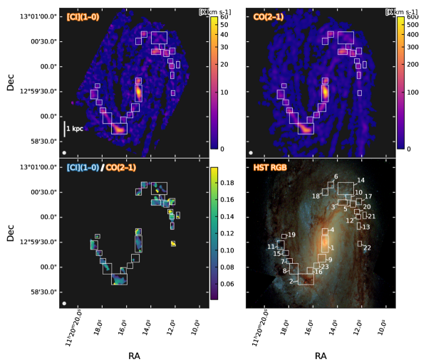
Figure 1: Top panels: NGC 3627 $[\mathrm{C}\,{\text{\sc{i}}}]\,(1\textnormal{--}0)$ (left) and $\mathrm{CO}\,(2\textnormal{--}1)$ (right) integrated line intensity (moment-0) maps within our broad mask (representing high-completeness signals; see Appendix A). Bottom left panel: $[\mathrm{C}\,{\text{\sc{i}}}]\,(1\textnormal{--}0)/\mathrm{CO}\,(2\textnormal{--}1)$ line ratio map within the combined signal mask. Bottom right panel: HST F814W-F555W-F438W RGB composite image (PHANGS-HST; Lee et al. 2022). Regions marked with the white boxes and labeled with numbers are mainly for illustration purpose and for discussion in the text. Their zoom-in images and extracted spectra are provided in our online data release. Examples for Regions 1, 4 and 22 are presented in Appendix D. All images have the same field of view of $179^{\prime\prime}\times 179^{\prime\prime}$, or $9.83\,\mathrm{kpc}\times 9.83\,\mathrm{kpc}$.

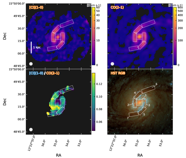
Figure 2: Similar to Fig. 1, the $[\mathrm{C}\,{\text{\sc{i}}}]\,(1\textnormal{--}0)$ and CO(2–1) moment-0 intensity maps and the line ratio map and the HST composite RGB image for NGC 4321. The field of view is $78^{\prime\prime}\times 78^{\prime\prime}$, or $5.75\,\mathrm{kpc}\times 5.75\,\mathrm{kpc}$.

2.3 ALMA observations of the additional targets from the literature

The NGC 1808 ALMA $[\mathrm{C}\,{\text{\sc{i}}}]\,(1\textnormal{--}0)$, $\mathrm{CO}\,(1\textnormal{--}0)$ and $\mathrm{CO}\,(2\textnormal{--}1)$ observations are presented in Salak et al. (2019) and all are interferometry plus total power, i.e., 12m+7m+tp, thus having no missing flux issue. To study the C i/CO line ratio consistently with our main targets, we only used the $[\mathrm{C}\,{\text{\sc{i}}}]\,(1\textnormal{--}0)$ and $\mathrm{CO}\,(2\textnormal{--}1)$ data. We re-reduced the raw data under ALMA project 2017.1.00984.S (PI: D. Salak) with the observatory calibration pipeline, then imaged, primary-beam-corrected and short-spacing-corrected using the PHANGS-ALMA pipeline in the same way as for our main targets (Appendix A). Note that in this step we re-reduced and imaged the total power data with the PHANGS-ALMA singledish pipeline (Herrera et al. 2020; Leroy et al. 2021a) and did the short-spacing correction with the PHANGS-ALMA pipeline right after the primary beam correction. The properties of the final CO-C i beam-matched data cubes are listed in Table 1.

The NGC 7469 ALMA data are presented in Izumi et al. (2020) and we used the archival raw data of $[\mathrm{C}\,{\text{\sc{i}}}]\,(1\textnormal{--}0)$ and $\mathrm{CO}\,(2\textnormal{--}1)$ under ALMA project 2017.1.00078.S (PI: T. Izumi). These are single pointings toward the centre. $[\mathrm{C}\,{\text{\sc{i}}}]\,(1\textnormal{--}0)$ is observed with ACA 7m and $\mathrm{CO}\,(2\textnormal{--}1)$ with the 12m array, both without total power. We re-reduced the data following the same procedure as for NGC 3627 and NGC 4321 with the PHANGS-ALMA pipeline.

Our re-reduced $[\mathrm{C}\,{\text{\sc{i}}}]\,(1\textnormal{--}0)$ and CO(2–1) line intensity and ratio maps for these additional galaxies are shown in Fig. 3.

3 Results of the observed line ratios

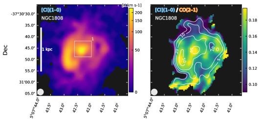
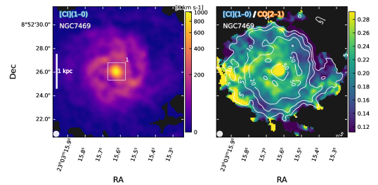
Figure 3: $[\mathrm{C}\,{\text{\sc{i}}}]\,(1\textnormal{--}0)$ (left) and $R_{{\mathrm{C\text{\sc{i}}}}/{\mathrm{CO}}}$ (right) maps of NGC 1808 in the upper panels and NGC 7469 in the lower panels. Similar to Figs. 1 and 2, the line intensity maps are defined in the broad mask and the $R_{{\mathrm{C\text{\sc{i}}}}/{\mathrm{CO}}}$ maps are restricted to the combined signal mask. Boxes in the left panels indicate the manually selected central regions where the pixels are highlighted in Fig. 4. Contours in the right panels indicate the 5, 10, 20 and 50-$\sigma$ levels of the left-panel C i intensity maps.

3.1 Spatial distributions

In Figs. 1, 2 and 3, we present the beam-matched $[\mathrm{C}\,{\text{\sc{i}}}]\,(1\textnormal{--}0)$ and $\mathrm{CO}\,(2\textnormal{--}1)$ integrated line intensity maps and their ratio maps. The C i/CO line ratio map is computed only for pixels within the joint strict mask area of the two lines, as described in Appendix A, representing high-confidence signals.

In NGC 3627 (Fig. 1), we visually marked 23 regions based on the C i and CO commonly-detected ($\mathrm{S/N}>3$), strict-mask areas for later analysis. Region IDs are sorted by their $[\mathrm{C}\,{\text{\sc{i}}}]\,(1\textnormal{--}0)$ brightness. Region 1 corresponds to the galaxy centre, Regions 2 and 3 are the southern and northern bar ends, Region 4 is an offset peak next to the galaxy centre, and other regions are mostly on the spiral arms. Most of these regions show a similar $R_{{\mathrm{C\text{\sc{i}}}}/{\mathrm{CO}}}\sim 0.1$, except for, e.g., Regions 20 and 22 which exhibit a somewhat higher ratio of $R_{{\mathrm{C\text{\sc{i}}}}/{\mathrm{CO}}}\sim 0.5$. The edge of Region 4 also shows an enhancement of C i yet it is hard to tell whether this is physical or simply caused by edge effects, e.g., as seen in our simulations (Appendix C).

We also examined the integrated spectra of each region in Appendix D. The C i and CO line profiles are not always well-matched in width and shape. In the galaxy centre (Region 1) and at bright bar-ends (Regions 2, 3, 5), C i and CO have similar line widths but C i has a lower intensity than CO, whereas in some fainter regions (9, 10, 13, 14), C i is narrower than CO and relatively weaker. In Regions 4, 20 and 22 where $R_{{\mathrm{C\text{\sc{i}}}}/{\mathrm{CO}}}$ is high, C i and CO have similar line widths but the C i intensity is enhanced.

In NGC 4321 (Fig. 2), we mapped a smaller area due to its fainter CO brightness than NGC 3627. There are no regions with $\mathrm{CO}\,(2\textnormal{--}1)$ integrated intensities $>100\,\mathrm{K\,km\,s^{-1}}$ outside our selected area in NGC 4321, whereas in comparison the NGC 3627 bar ends have $\mathrm{CO}\,(2\textnormal{--}1)$ integrated intensities $\gtrsim 300\,\mathrm{K\,km\,s^{-1}}$. The C i mapping in NGC 4321 has a similar depth as in NGC 3627.

We marked 7 regions in NGC 4321 to guide the visual inspection. A clear $R_{{\mathrm{C\text{\sc{i}}}}/{\mathrm{CO}}}$ deficit can be seen in the galaxy centre (Region 1), with $R_{{\mathrm{C\text{\sc{i}}}}/{\mathrm{CO}}}\sim 0.06$, nearly a factor of two smaller than its inner disk which has similar $R_{{\mathrm{C\text{\sc{i}}}}/{\mathrm{CO}}}\sim 0.1$ as seen in the NGC 3627 disk. Some C i enhancement can be found at the edges or slightly outside these regions, where CO and C i are both faint ($I_{\mathrm{CO}\,(2\textnormal{--}1)}\sim 30-100\,\mathrm{K\,km\,s^{-1}}$) and the edge effect of interferometric missing flux might play a role (see Appendix C).

The $R_{{\mathrm{C\text{\sc{i}}}}/{\mathrm{CO}}}$ spatial distributions of the other two starburst/AGN galaxies (Fig. 3) show in general more enhanced $R_{{\mathrm{C\text{\sc{i}}}}/{\mathrm{CO}}}$ than in the NGC 3627 and NGC 4321 disks. Large variations from the centres to outer areas can be seen, especially at the the S/N threshold of $\sim 3\text{--}5$ (see contours).

To quantify the spatial co-localization of the C i and CO emission, we use the JACoP tool (Bolte & Cordelières 2006)  in the ImageJ software (Schneider et al. 2012) to measure the commonly used co-localization indicators, namely the Pearson’s coefficient (PC; equal to 0 and 1 for null and 100% localization, respectively) and Manders’ coefficients (M1 and M2; which measure the overlap between two images and are equal to one for perfect overlap). We turn on the option of using Costes’ automatic threshold (Costes et al. 2004) which automatically set a pixel value threshold for each image to minimize the contribution of noise for the comparison (Bolte & Cordelières 2006). For the C i and CO emission in our galaxies, we find $\mathrm{PC/M1/M2}$ values all very close to 1, that is, nearly 100% co-localization ($\mathrm{PC/M1/M2}=0.934/0.985/0.990$ for NGC 3627, $0.816/0.986/0.964$ for NGC 4321, $0.978/0.890/0.906$ for NGC 1808, and $0.935/0.999/0.998$ for NGC 7469).

Overall, the spatial comparison of the C i and CO intensities demonstrates that the two species are well-correlated when observed at hundred parsec scales. Meanwhile, we do see certain spectral differences in the line profiles as shown in Appendix D. This may suggest that variations exist at smaller scales than our resolution, which could be the sign of different evolutionary stages (e.g. Kruijssen & Longmore 2014) and would be interesting for higher-resolution follow-ups, e.g., with the main ALMA 12m array.

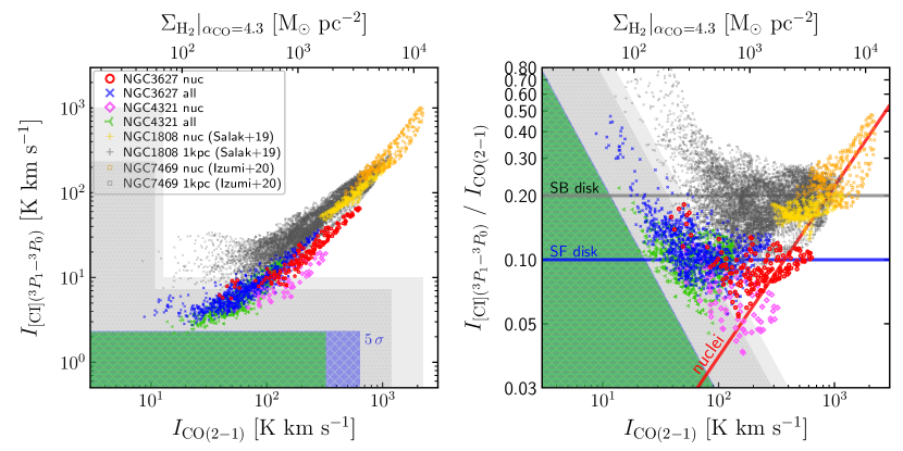
Figure 4: Left: $I_{[\mathrm{C}\,{\text{\sc{i}}}]\,(1\textnormal{--}0)}$ versus $I_{\mathrm{CO}\,(2\textnormal{--}1)}$ in the four galaxies we studied: NGC 3627, NGC 4321, NGC 1808 and NGC 7469. $I_{[\mathrm{C}\,{\text{\sc{i}}}]\,(1\textnormal{--}0)}$ and $I_{\mathrm{CO}\,(2\textnormal{--}1)}$ integrated fluxes are moment-0 intensities extracted from their beam and pixel size matched data cubes. Only data points with propagated moment-0 $\mathrm{S/N}\geq 5$ are shown. The blue (with crossed hatch), green (with horizontal line hatch), gray (with dotted hatch) and light gray shadings indicate the $5\,\sigma$ thresholds for the four galaxies, respectively. Typical line widths of 10 km s^-1 (NGC 3627 and NGC 4321) and 30 km s^-1 (NGC 1808 and NGC 7469) in sigma are used to calculate the thresholds together with the channel rms in Table 1. For NGC 3627 and NGC 4321, their ($uv$-matched) CO(2–1) $5\,\sigma$ thresholds are out of the plotting range. Top axis shows the simply-converted H₂ surface density using a constant $\alpha_{\mathrm{CO}}=4.3$ and CO excitation (i.e., CO(2–1) to CO(1–0) line ratio) $R_{21}=0.65$. Right: Same data but shown as the line ratio $R_{{\mathrm{C\text{\sc{i}}}}/{\mathrm{CO}}}=I_{[\mathrm{C}\,{\text{\sc{i}}}]\,(1\textnormal{--}0)}/I_{\mathrm{CO}\,(2\textnormal{--}1)}$ versus $I_{\mathrm{CO}\,(2\textnormal{--}1)}$. The blue horizontal line indicates a star-forming (SF) disk-like $R_{{\mathrm{C\text{\sc{i}}}}/{\mathrm{CO}}}\sim 0.1$, i.e., the spiral arms of NGC 3627 and NGC 4321. The gray horizontal line indicates a starburst (SB) disk-like $R_{{\mathrm{C\text{\sc{i}}}}/{\mathrm{CO}}}\sim 0.2$, i.e., the $\sim 1$ kpc SB disk/ring in NGC 1808 and NGC 7469. The red line with a slope of 0.8 in logarithm ($0.035\,(I_{\mathrm{CO}\,(2\textnormal{--}1)}/[100\,\mathrm{K\,km\,s^{-1}}])^{0.8}$) visually guides the trend of increasing $R_{{\mathrm{C\text{\sc{i}}}}/{\mathrm{CO}}}$ in the central regions of these galaxies (see boxes in Figs. 1 to 3, sizes $\sim 300$–500 pc).

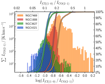
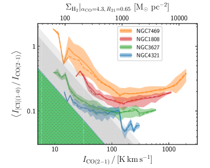
Figure 5: Left panel shows the histograms of the sum of CO(2–1) surface brightness over pixels in each C i/CO line ratio interval in the four galaxies. The bold curves are the cumulative distributions of the corresponding histograms. Right panel shows the mean C i/CO line ratio for pixels in each bin of CO(2–1) surface brightness (or molecular gas surface density as indicated by the top-axis assuming a constant $\alpha_{\mathrm{CO}}=4.3$ and $R_{21}=0.65$). Shaded area enveloping each mean trend indicates the 16- to 84-th percentiles in each bin, and dashed line indicates the 50-th percentile. This panel thus more clearly illustrates the ridge and scatter of the trends in the right panel of Fig. 4. Detection limits are shown consistently with Fig. 4.

3.2 $R_{{\mathrm{C\text{\sc{i}}}}/{\mathrm{CO}}}$ versus CO surface brightness and gas surface density

In Fig. 4 we show the scatter points of C i and CO line brightnesses and the $R_{{\mathrm{C\text{\sc{i}}}}/{\mathrm{CO}}}$ line ratios. Systematic differences in $R_{{\mathrm{C\text{\sc{i}}}}/{\mathrm{CO}}}$ can be found among these galaxies and within their galactic environments. We discuss these environments separately as follows.

3.2.1 Star-forming and starburst disk environments

The majority of molecular gas in the 3–7 kpc star-forming disks of NGC 3627 and NGC 4321 exhibits a tight distribution of $R_{{\mathrm{C\text{\sc{i}}}}/{\mathrm{CO}}}$ around 0.1 (within about $\pm$50%). The distribution is fairly flat over an order of magnitude in $I_{\mathrm{CO}\,(2\textnormal{--}1)}$. We denote this as the “SF disk” regime. The ratio rises to about 0.2 within a galactocentric radius of few hundred parsec to $\sim 1$ kpc starburst areas in NGC 1808 and NGC 7469, which we define as the “SB disk” regime.

The nearly flat “SB disk” distribution is consistent with earlier studies. Salak et al. (2019) found that in NGC 1808 $I_{[\mathrm{C}\,{\text{\sc{i}}}]\,(1\textnormal{--}0)}$ is proportional to $I_{\mathrm{CO}\,(2\textnormal{--}1)}^{\ +1.05}$. They also studied CO(1–0), finding that $I_{[\mathrm{C}\,{\text{\sc{i}}}]\,(1\textnormal{--}0)}\propto I_{\mathrm{CO}\,(1\textnormal{--}0)}^{\ +1.46}$, i.e., with a steeper slope. Saito et al. (2020) found a similar slope between $I_{[\mathrm{C}\,{\text{\sc{i}}}]\,(1\textnormal{--}0)}$ and $I_{\mathrm{CO}\,(1\textnormal{--}0)}$: $I_{[\mathrm{C}\,{\text{\sc{i}}}]\,(1\textnormal{--}0)}\propto I_{\mathrm{CO}\,(1\textnormal{--}0)}^{\ +1.54}$ in IRAS F18293-3413 (whose CO(2–1) data is insufficient for such a study as previously mentioned). This correlation slope is likely to change with different CO transitions due to the CO excitation’s dependence on the CO luminosity or star formation rate themselves (e.g., Daddi et al. 2015; Liu et al. 2021). For higher-$J$ CO transitions, Michiyama et al. (2021) studied C i and CO(4–3) lines in 36 (U)LIRGs, finding $I_{[\mathrm{C}\,{\text{\sc{i}}}]\,(1\textnormal{--}0)}\propto I_{\mathrm{CO}\,(4\textnormal{--}3)}^{\ +0.97}$.

The upward tails seen at the CO-faint-end in the right panel of Fig. 4 are mostly due to the detection limits in each galaxy. The color shading indicates the 5-$\sigma$ limit for each galaxy, assuming a typical line width of 10 km s^-1. Region 22 of NGC 3627 and the outer pixels in the two starburst/AGN galaxies make the tips of the blue and gray faint-end tails, respectively. But most of these features should still be spurious. We performed CASA simulations following the real observations of NGC 3627 to verify what we would get if $R_{{\mathrm{C\text{\sc{i}}}}/{\mathrm{CO}}}$ were constant across the galaxies (Appendix C) We find that noise can indeed boost a simulated $R_{{\mathrm{C\text{\sc{i}}}}/{\mathrm{CO}}}$ of 0.2 to a measurement as high as 0.5 in a NGC 3627-like large mosaic, or even higher to $>1$ in single-pointing ALMA data without total power or sufficient short spacing. However, the faint-end tail from the simulation is not very similar to that of NGC 3627, raising some questions about the nature of the high-$R_{{\mathrm{C\text{\sc{i}}}}/{\mathrm{CO}}}$ in Region 22.

Furthermore, we also did stacking experiments using the CO line profile as the prior to measure the C i line fluxes in bins of CO line brightnesses or galactocentric radii. We find no systematically higher $R_{{\mathrm{C\text{\sc{i}}}}/{\mathrm{CO}}}$ at fainter CO pixels or at the outer radii.

3.2.2 Galaxy centre environments

Most interestingly, the $\lesssim 250$ pc centres of all four galaxies show dramatically different $R_{{\mathrm{C\text{\sc{i}}}}/{\mathrm{CO}}}$. It varies by a factor of ten from $\sim 0.05$ in the centre of NGC 4321 to $\sim 0.1$ in the centre of NGC 3627, then to $\sim 0.15$–0.2 at the centre of NGC 1808, and to $\sim 0.2$–0.5 in the nucleus of NGC 7469. This “nuclei” trend has a slope of about 0.8, i.e., $I_{[\mathrm{C}\,{\text{\sc{i}}}]\,(1\textnormal{--}0)}\approx 0.035\;I_{\mathrm{CO}\,(2\textnormal{--}1)}^{\ +0.8}$, and corresponds to a $\Sigma_{\mathrm{mol}}$ range of about $10^{3}$ to $10^{4}\;\mathrm{M_{\odot}\,pc^{-2}}$ if adopting an $\alpha_{\mathrm{CO}}=4.3\ \mathrm{M_{\odot}\;(K\,km\,s^{-1}\,pc^{2})^{-1}}$ (Bolatto et al. 2013) and a CO excitation $R_{21}=0.65$ (Leroy et al. 2022).

The reasons for the nuclei showing this trend likely include both the effect of varying [C i/CO] abundance ratio and the excitation and radiative transfer. They are determined by the actual ISM conditions in each environment, i.e., the gas kinetic temperature, C i and CO column densities ($N_{\mathrm{C\text{\sc{i}}}}$ and $N_{\mathrm{CO}}$), line widths ($\Delta{v}$), and $\mathrm{H_{2}}$ volume density ($n_{\mathrm{H_{2}}}$), etc. They will be analyzed in Sect. 4.

3.2.3 Histogram and curve-of-growth of the line ratio distributions

Fig. 5 shows the histogram and cumulative distribution functions of $R_{{\mathrm{C\text{\sc{i}}}}/{\mathrm{CO}}}$ (left panel) and the mean $R_{{\mathrm{C\text{\sc{i}}}}/{\mathrm{CO}}}$ and the 16-th to 84-th percentiles in bins of CO line intensity (right panel) in our galaxies. The histogram is computed as the sum of CO line intensity in each bin of $R_{{\mathrm{C\text{\sc{i}}}}/{\mathrm{CO}}}$, representing the amount of gas at each $R_{{\mathrm{C\text{\sc{i}}}}/{\mathrm{CO}}}$. The NGC 4321 histogram is lower than others, showing that it has the least total molecular gas mass among the four galaxies within mapped areas. The NGC 3627 histogram has a peak about 0.5 dex higher than that of NGC 4321, but their peak locations are consistently at $\log R_{{\mathrm{C\text{\sc{i}}}}/{\mathrm{CO}}}\sim-1$, same conclusion as our previous scatter plots show. The two SB galaxies NGC 1808 and NGC 7469, despite having much smaller observed areas ($\sim 1$–$2$ kpc), have more than an order of magnitude higher peaks hence total molecular gas masses. The locations of their histogram peaks also shift to a systematically higher $R_{{\mathrm{C\text{\sc{i}}}}/{\mathrm{CO}}}$. It is clearly seen that both SF and SB disks lack a high-$R_{{\mathrm{C\text{\sc{i}}}}/{\mathrm{CO}}}$ ($\log R_{{\mathrm{C\text{\sc{i}}}}/{\mathrm{CO}}}>-0.35$) gas component which dominates the gas in the strong AGN host galaxy NGC 7469.

The curve-of-growth in the left panel of Fig. 5 further shows the cumulative CO brightness in bins of $R_{{\mathrm{C\text{\sc{i}}}}/{\mathrm{CO}}}$, and reflects the fact that the majority of gas in our galactic disks has a narrow distribution of $R_{{\mathrm{C\text{\sc{i}}}}/{\mathrm{CO}}}$ (see also last few rows in Table 1). In NGC 3627, NGC 4321 and NGC 1808, the higher- and lower-$R_{{\mathrm{C\text{\sc{i}}}}/{\mathrm{CO}}}$ gas outside $\pm 0.1$ dex around the mean $R_{{\mathrm{C\text{\sc{i}}}}/{\mathrm{CO}}}$ only sums up to $<5$–$10\%$ of their total gas masses.

In the right panel of Fig. 5, we illustrate how the mean $R_{{\mathrm{C\text{\sc{i}}}}/{\mathrm{CO}}}$ changes with different gas surface density, as well as the scatter of the data point distribution. The 2D pixels are binned by CO brightness, and the mean and 16%/50%/84%-th percentiles of the $R_{{\mathrm{C\text{\sc{i}}}}/{\mathrm{CO}}}$ are computed for each bin. It sketches out the mean trends in Fig. 4 (right panel), and also reveals that a) the scatter of $R_{{\mathrm{C\text{\sc{i}}}}/{\mathrm{CO}}}$ is the largest ($\pm 0.20$ dex) in the starburst disk of NGC 7469 compared to other galaxies; b) the scatter is the smallest ($\pm 0.06$ dex) in the star-forming disks of NGC 4321 and NGC 3627 where $\Sigma_{\mathrm{mol}}\sim 100\text{--}500\;\mathrm{M_{\odot}\,pc^{-2}}$; c) the scatters are very similarly ($\pm 0.10$ dex) at a relatively high $\Sigma_{\mathrm{mol}}\sim 1000\;\mathrm{M_{\odot}\,pc^{-2}}$ in all our galaxies except for NGC 4321’s centre.

3.3 $R_{{\mathrm{C\text{\sc{i}}}}/{\mathrm{CO}}}$ versus ISRF

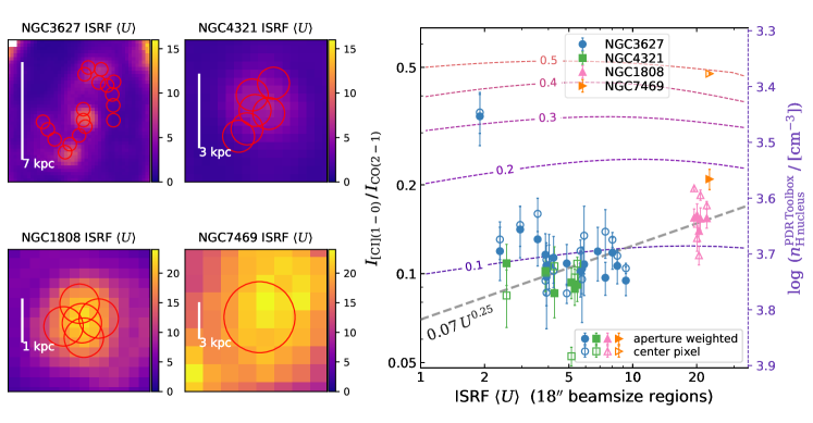
Figure 6: Line ratio versus mean ISRF intensity $\left<U\right>$ measured from SED fitting to the near- to far-IR (Spitzer, Herschel) data. Left four panels are the $\left<U\right>$ maps of NGC 3627, NGC 4321, NGC 1808 and NGC 7469, and as described in Sect. 3.3 are obtained from the works done by J. Chastenet et al. (in prep.) as a continued effort of Chastenet et al. (2021). Right panel shows the scatter plot of $R_{{\mathrm{C\text{\sc{i}}}}/{\mathrm{CO}}}$ versus $\left<U\right>$ at a spatial resolution of $\sim 18^{\prime\prime}$ in the manually-selected apertures shown in the left panels. We computed a beam-weighted mean $R_{{\mathrm{C\text{\sc{i}}}}/{\mathrm{CO}}}$ and a centre pixel $R_{{\mathrm{C\text{\sc{i}}}}/{\mathrm{CO}}}$ for each aperture, displayed as the solid and open symbols, respectively. Error bars are the corresponding beam-weighted mean or central pixel $R_{{\mathrm{C\text{\sc{i}}}}/{\mathrm{CO}}}$ uncertainties in each region. The region diameter ($\sim 18^{\prime\prime}$) corresponds to the coarsest resolution of the Herschel data used in the SED fitting. The gray dotted line shows $R_{{\mathrm{C\text{\sc{i}}}}/{\mathrm{CO}}}=0.07\,U^{0.25}$ as a guiding line. The colored dotted contours (labeled 0.1–0.5) are the model contours of $R_{{\mathrm{C\text{\sc{i}}}}/{\mathrm{CO}}}$ computed from the PDR Toolbox (using the latest wk2020 model and solar metallicity; Kaufman et al. 2006). We convert $G_{0}$ from the model contour to the $x$-axis $U$ by multiplying with a factor of 0.88 (Draine et al. 2007). The right $y$-axis indicates the PDR model’s $n_{\mathrm{H_{2}}}$, whose range is manually adjusted so that the model contours roughly match the left $x$-axis. The PDR model contours show little dependence of $R_{{\mathrm{C\text{\sc{i}}}}/{\mathrm{CO}}}$ on $U$ in the horizontal direction but a strong correlation with $n_{\mathrm{H_{2}}}$ as seen by the vertical gradient.

Here we study how $R_{{\mathrm{C\text{\sc{i}}}}/{\mathrm{CO}}}$ correlates with the interstellar radiation field (ISRF) intensity ($U$; in units of Milky Way mean ISRF; Habing 1968), which is a measure of the UV radiation field strength impacting the ISM. Since C i originates from PDRs, its abundance should be highly related to the PDR properties, thus whether or how $R_{{\mathrm{C\text{\sc{i}}}}/{\mathrm{CO}}}$ correlates with the ISRF that illuminates the PDR is a key question.

The ISRF intensity $U$ is usually measured by the re-radiated dust emission, as the original UV photons are highly attenuated by dust in the ISM. Draine & Li (2007, hereafter DL07) developed a series of dust grain models and synthesized SED templates that can describe nearby galaxies’ observed dust SEDs. A number of studies (e.g., Draine et al. 2007; Galliano et al. 2011; Dale et al. 2012; Aniano et al. 2012, 2020; Daddi et al. 2015; Chastenet et al. 2017; Liu et al. 2021; Chastenet et al. 2021) have used the DL07 models to fit the dust SEDs of galaxies near and far.

For our study, we adopt the mass-averaged ISRF $\left<U\right>$ maps from an ongoing effort by J. Chastenet et al. (in prep.) which is a continuation of the work published for other galaxies by Chastenet et al. (2017, 2021) with the same method. In this method, the Herschel far-infrared, Spitzer and/or WISE near-infrared images  are first PSF-matched to a common resolution $\sim 18^{\prime\prime}$ (Herschel SPIRE 250$\mu$m), then SED fitting is performed using the DL07 models at each pixel. Each dust SED is fitted by two dust components, one in the ambient ISM with a constant ISRF intensity $U_{\mathrm{min}}$, and the other in regions with higher $U$ with a power law distributed ISRF from $U_{\mathrm{min}}$ up to $U_{\mathrm{max}}=10^{7}$. The fitting then gives the best-fit $U_{\mathrm{min}}$ and the power-law index $\gamma$ of the $U$ distribution. The mean ISRF intensity $\left<U\right>$ is calculated as the dust mass-weighted mean of the ambient and power-law ISRF intensities (in DL07, $U_{\rm PDR}\geq 10^{2}$ is considered to be associated with the PDR), and better represents the overall ISRF than $U_{\mathrm{min}}$.

Fig. 6 presents the $\left<U\right>$ maps and the $R_{{\mathrm{C\text{\sc{i}}}}/{\mathrm{CO}}}$ versus $\left<U\right>$ scatter plot. Since the spatial resolution of the $\left<U\right>$ maps is $18^{\prime\prime}$, we calculate a weighted $R_{{\mathrm{C\text{\sc{i}}}}/{\mathrm{CO}}}$ in each circular aperture shown in Fig. 6 whose diameter equals the $\left<U\right>$ map resolution, with weighting following the 2D Gaussian beam. In addition, we also show the central pixel value for each region in Fig. 6. We restrict the analysis to regions where both $\left<U\right>$ and $R_{{\mathrm{C\text{\sc{i}}}}/{\mathrm{CO}}}$ are measured.

A weak correlation between $R_{{\mathrm{C\text{\sc{i}}}}/{\mathrm{CO}}}$ and $\left<U\right>$ is seen from the SF to SB disks, with a large scatter. For reference, we plot a $R_{{\mathrm{C\text{\sc{i}}}}/{\mathrm{CO}}}=0.07\,U^{0.25}$ line to indicate this weak trend. The lowest-$\left<U\right>$ data point in NGC 3627 (mainly Region 22) and the centre of NGC 7469 do not follow this trend, possibly indicating other C i enhancement mechanisms than $\left<U\right>$.

We use the popular PDR modelling software, PDR Toolbox (version 2.2.9; Kaufman et al. 2006; Pound & Wolfire 2008, 2011)  to compute the theoretical $R_{{\mathrm{C\text{\sc{i}}}}/{\mathrm{CO}}}$ in uniform grids of ISRF intensity in the Habing (1968) $G_{0}$ unit and H nucleus density $n_{\mathrm{H}}$ (both in log space). We adopt the latest wk2020 model set and a solar metallicity ($\mathrm{[O/H_{2}]}=3.2\times 10^{-4}$, $\mathrm{[C/H_{2}]}=1.6\times 10^{-4}$). The ISRF intensity grid can be directly scaled to $U$ by multiplying a factor 0.88 (Draine et al. 2007), corresponding to the $x$-axis of Fig. 6. The $n_{\mathrm{H}}$ grid is not directly linked to the left $y$-axis of Fig. 6, but because the model contours show fairly flat $R_{{\mathrm{C\text{\sc{i}}}}/{\mathrm{CO}}}$ versus $U$ trends, we can match the model contours and indicate the $n_{\mathrm{H}}$ grid in the right $y$-axis of Fig. 6.

The PDR modelling predicts generally flat $R_{{\mathrm{C\text{\sc{i}}}}/{\mathrm{CO}}}$ versus $U$ trends similar to the distribution of the observed data points, although our $U$ are diluted values at a much larger physical scale than in the PDR models. However, in PDR models, $R_{{\mathrm{C\text{\sc{i}}}}/{\mathrm{CO}}}$ changes moderately with $n_{\mathrm{H}}$, and a relatively high $n_{\mathrm{H}}\sim 10^{3.5\text{--}3.7}\,\mathrm{cm^{-3}}$ is needed to reproduce an $R_{{\mathrm{C\text{\sc{i}}}}/{\mathrm{CO}}}\sim 0.1$–0.2, or equivalently $\sim 1.0$–1.9 for the ratio of $[\mathrm{C}\,{\text{\sc{i}}}]\,(1\textnormal{--}0)$ and $\mathrm{CO}\,(2\textnormal{--}1)$ fluxes in $\mathrm{erg\,s^{-1}\,cm^{-2}\,sr^{-1}}$ units used by the PDR Toolbox . Furthermore, the PDR model needs a $\sim 0.5$ dex lower $n_{\mathrm{H}}$ to explain the $2\times$ elevated $R_{{\mathrm{C\text{\sc{i}}}}/{\mathrm{CO}}}$ in SB disks, which seems somewhat counterintuitive.

This apparent tension is likely caused by the observations probing a much coarser resolution that consists of a large number of PDRs with different $n_{\mathrm{H}}$ and $U$ (e.g., increasing $U$ from 10 to 400 can increase $R_{{\mathrm{C\text{\sc{i}}}}/{\mathrm{CO}}}$ from 0.2 to 0.5 based on our PDR Toolbox modelling). It may also relate to an abundance variation driven by non-PDR mechanisms — X-ray dominated region (XDR; Maloney et al. 1996; Meijerink & Spaans 2005; Meijerink et al. 2007; see also review by Wolfire et al. 2022) and Cosmic Ray Dominated Region (CRDR; Papadopoulos 2010; Papadopoulos et al. 2011, 2018; Bisbas et al. 2015, 2017) are well-known to play an important role in starbursting and AGN environments, respectively.

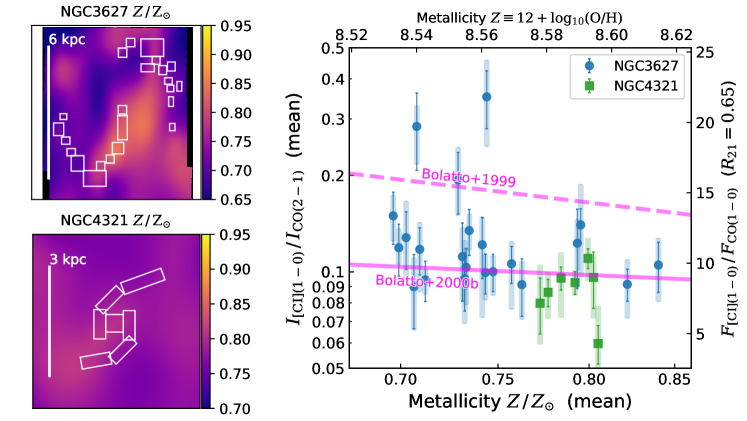
Figure 7: Left two panels show the metallicity maps of NGC 3627 and NGC 4321 from Williams et al. (2022) based on PHANGS-MUSE (Emsellem et al. 2022) data. Boxes are regions as defined in Figs. 1 and 2. Right panel shows the $R_{{\mathrm{C\text{\sc{i}}}}/{\mathrm{CO}}}$ versus metallicity scatter plot for regions in NGC 3627 and NGC 4321. The bottom-axis is metallicity in solar units, top-axis is metallicity in $12+\log(\mathrm{O/H})$, left-axis is the line ratio of $[\mathrm{C}\,{\text{\sc{i}}}]\,(1\textnormal{--}0)$ and $\mathrm{CO}\,(2\textnormal{--}1)$ in $\mathrm{K\,km\,s^{-1}}$ units, and right-axis is the ratio of fluxes in $\mathrm{erg\,s^{-1}\,cm^{-2}\,sr^{-1}}$ units. The left- and right-axes are matched by a factor of $(\nu_{\mathrm{C{\textsc{i}}1\textnormal{--}0}}/\nu_{\mathrm{CO1\textnormal{--}0}})^{3}\times R_{21}$, where we adopt a $R_{21}=0.65$ (Leroy et al. 2022). Data points are the mean metallicity and $R_{{\mathrm{C\text{\sc{i}}}}/{\mathrm{CO}}}$ in each region shown in left panels, with error bars indicating the typical uncertainty in $R_{{\mathrm{C\text{\sc{i}}}}/{\mathrm{CO}}}$, and vertical color shading indicating the 16- to 84-th percentiles of pixels’ $R_{{\mathrm{C\text{\sc{i}}}}/{\mathrm{CO}}}$ distribution inside each region. The Bolatto et al. (2000b) empirical fitting and Bolatto et al. (1999) model prediction lines are overlaid. The three outliers in NGC 3627 with $R_{{\mathrm{C\text{\sc{i}}}}/{\mathrm{CO}}}\sim 0.19$, 0.28 and 0.35 are Regions 20, 21 and 22, respectively. The outlier point in NGC 4321 with $R_{{\mathrm{C\text{\sc{i}}}}/{\mathrm{CO}}}\sim 0.06$ is its centre Region 1.

As pointed out by Papadopoulos et al. (2011) and later works, ultra-luminous infrared galaxies (ULIRGs) with IR luminosities $L_{\mathrm{IR,\,8-1000\mu\mathrm{m}}}\geq 10^{12}\,\mathrm{L_{\odot}}$ and corresponding $\mathrm{SFRs}>1000\,\mathrm{M_{\odot}\,yr^{-1}}$ have cosmic-ray (CR) energy densities $\sim 10^{3}\text{--}10^{4}\times$ larger than the Milky Way. In our sample, the two SB galaxies are not as intensively star-forming as ULIRGs, but their SFRs are still a factor of 2 to 20 higher than our SF galaxies. More importantly, the SB disks have considerably higher (e.g., one to two orders of magnitude) SFR surface densities than the SF disks, plausibly leading to a factor of a few tens to hundreds higher CR intensities. The CRs emitted from OB star clusters and supernova remnants can penetrate deeply into the ISM, and thus nearly uniformly illuminate the ISM and effectively dissociate CO into C i.

A detailed simulation by Bisbas et al. (2017) showed that $10\times$ and $100\times$ higher CR ionization rates ($\xi_{\mathrm{CR}}$) than the Milky Way level results into a factor of about 2 and 3 mildly-increased C i abundance and about 1/2 and 1/30 strongly-decreased CO abundance, respectively (see their Fig. 3), in a 10 pc GMC with a mean gas density $\left<n_{\mathrm{H}}\right>=760\,\mathrm{cm^{-3}}$, resembling Milky Way and typical SF galaxies’ ISM conditions. Our SB galaxies probably have a $\xi_{\mathrm{CR}}$ around or slightly above 10, but not reaching 100 given their mild $\left<U\right>\sim 20-30$ compared to the $\left<U\right>\gtrsim 50$ in extreme SB galaxies, e.g., local ULIRGs and high-redshift hyperluminous IR-bright (HyLIRG) and submm galaxies (Daddi et al. 2015; Silverman et al. 2018; Liu et al. 2021). In Sect. 4, we show that the mildly-increased [C i/CO] abundance ratio from a CRDR and temperature/density-driven excitation can lead to the factor of 2 increase in $R_{{\mathrm{C\text{\sc{i}}}}/{\mathrm{CO}}}$ when going from SF to SB disks.

3.4 $R_{{\mathrm{C\text{\sc{i}}}}/{\mathrm{CO}}}$ versus Metallicity

Our current sample covers a relatively small range in metallicity for a metallicity–line ratio study. Given their stellar masses and metallicity maps (e.g., Kreckel et al. 2019, 2020; Williams et al. 2022), our targets probe a near-solar metallicity. NGC 3627 has a well-measured metallicity gradient of $Z=8.53+0.06\times[r/R_{25}]$ from Kreckel et al. (2019) , but the metallicity of individual H ii regions scatter between $\sim 8.45$–$8.65$. Williams et al. (2022) produced the 2D spatial distributions of gas-phase metallicity in PHANGS-MUSE galaxies, including NGC 3627 and NGC 4321, by applying the Gaussian Process Regression to map the smooth, higher-order metallicity variation from the individual, sparse H ii regions detected in PHANGS-MUSE (Emsellem et al. 2022; Santoro et al. 2022). This method is significantly superior to a naïve nearest neighbor interpolation method. We refer the reader to Williams et al. (2022) for the technical details and validation demonstration.

In Fig. 7 we present the trend between $R_{{\mathrm{C\text{\sc{i}}}}/{\mathrm{CO}}}$ and metallicity in NGC 3627 and NGC 4321. Due to our limited metallicity range, only a very weak decreasing trend can be seen. A similar trend has been reported by Bolatto et al. (2000b), who observed CO(1–0) and $[\mathrm{C}\,{\text{\sc{i}}}]\,(1\textnormal{--}0)$ in the Region N27 of the Small Magellanic Cloud and combined with literature data to present a correlation between $R_{{\mathrm{C\text{\sc{i}}}}/{\mathrm{CO}}}$ and metallicity over $\sim 0.2\text{--}2\,Z_{\odot}$. We overlay the Bolatto et al. (2000b) empirical fitting  as well as a theoretical PDR model prediction line from Bolatto et al. (1999) in Fig. 7. Although our data covers only a small metallicity range, it is encouraging to see the overall good agreement with the observationally-driven trend in Bolatto et al. (2000b). More detailed understanding of the deviation from PDR models will likely need more C i mapping in lower-metallicity galaxies.

4 Estimation of abundance ratios under representative ISM conditions

The observed $R_{{\mathrm{C\text{\sc{i}}}}/{\mathrm{CO}}}$ depends on not only the C i and CO abundances ($\mathrm{[CO/H_{2}]}$ and $\mathrm{[C\text{\sc{i}}/H_{2}]}$), but also the ISM conditions that determine the excitation (level population) and radiative transfer of the C atoms and CO molecules — i.e., the gas kinetic temperature $T_{\mathrm{kin}}$, volume density of H₂ ($n_{\mathrm{H_{2}}}$; as the primary collision partners of C and CO), turbulent line width ${\Delta\text{v}}$, and the species’ column densities $N_{\mathrm{CO}}$ and $N_{\mathrm{C\text{\sc{i}}}}$. The column density divided by the line width ($N/{\Delta\text{v}}$) further determines the optical depth $\tau$ of each line.

In this work, having only a CO(2–1) and a $[\mathrm{C}\,{\text{\sc{i}}}]\,(1\textnormal{--}0)$ line is insufficient to numerically solve all the $T_{\mathrm{kin}}$, $n_{\mathrm{H_{2}}}$, $N_{\mathrm{CO}}/{\Delta\text{v}}$, $\mathrm{[CO/H_{2}]}$ and $\mathrm{[C\text{\sc{i}}/H_{2}]}$. Therefore, we assume several representative ISM conditions where $T_{\mathrm{kin}}$, ${\Delta\text{v}}$ and $\mathrm{[CO/H_{2}]}$ are fixed to reasonable values, then solve the $N_{\mathrm{CO}}$ and $N_{\mathrm{C\text{\sc{i}}}}$. We assume that C i and CO are spatially mixed at our resolution, i.e., they have the same filling factor. This is a relatively strong assumption and is likely not the real case, because although we see spatial co-localization at our $\sim 200$ pc resolutions, the spectral profiles of CO and C i show discrepancies (Appendix D), indicating different underlying distributions at smaller scales. With the assumption of the same filling factor (and 3D distribution), the column density ratio $N_{\mathrm{C\text{\sc{i}}}}/N_{\mathrm{CO}}$ equals the [C i/CO] abundance ratio.

We perform both LTE and non-LTE calculations. LTE assumes that all transitions are thermalized locally, and the level population follows Boltzmann statistics, so that each transition’s excitation temperature $T_{\mathrm{ex}}$ as defined by the level population equals $T_{\mathrm{kin}}$ (e.g., Spitzer 1998; Tielens 2010; Draine 2011). The LTE assumption facilitates the computation as we do not need to solve the level population and thus $n_{\mathrm{H_{2}}}$ is not used. However, LTE is not easily reached in typical ISM conditions. Subthermalized lines need non-LTE calculations. The commonly adopted non-LTE approach is the Large Velocity Gradient (LVG; Scoville & Solomon 1974; Goldreich & Kwan 1974), where an escape fraction is used to facilitate the local radiation intensity calculation hence the detailed balance of radiative and collisional (de-)excitations. We use RADEX (van der Tak et al. 2010) to compute the non-LTE C i and CO line fluxes for each fixed parameter set ($T_{\mathrm{kin}}$, $n_{\mathrm{H_{2}}}$, $N_{\mathrm{CO}}$, $N_{\mathrm{C\text{\sc{i}}}}$, ${\Delta\text{v}}$), then study how [C i/CO] determines the line flux ratio $R_{{\mathrm{C\text{\sc{i}}}}/{\mathrm{CO}}}$.

We assume the following 7 representative ISM conditions: (1) inner Galactic GMCs, (2) NGC 3627/4321 disk GMCs, (3) NGC 3627 bar-end environments, (4) NGC 1808/7469 SB disk, (5) NGC 4321 centre, (6) NGC 3627 centre, and (7) NGC 7469 centre. Conditions (1)–(3) correspond to the “SF disk” in Fig. 4, and condition (4) represents the “SB disk”. The last three conditions are for the “nuclei”. Under each ISM condition, we set a fixed $T_{\mathrm{kin}}$ (in units of K), ${\Delta\text{v}}$ (in units of km s^-1), $\mathrm{[CO/H_{2}]}$, and $\Sigma_{\mathrm{mol}}$ (in units of $\mathrm{M_{\odot}\,pc^{-2}}$). The adopted values are shown at the top of each panel in Figs. 8 and 9.

Our choice of $T_{\mathrm{kin}}$ considered multi-line measurements in the literature, e.g., Heyer & Dame (2015) for Galactic GMC ISM condition, and Teng et al. (2022) for NGC 3627 nucleus, as well as typical values in simulations (e.g., Offner et al. 2014; Glover et al. 2015; Glover & Clark 2016; Clark et al. 2019; Hu et al. 2021). Our ${\Delta\text{v}}$ is based on the observed line width in the highest-resolution ALMA data, i.e., from the original PHANGS-ALMA $1^{\prime\prime}$ data (Leroy et al. 2021b) or from Salak et al. (2019) and Izumi et al. (2020) for NGC 1808 and NGC 7469, respectively. The observed line width should at least provide an upper limit, if not directly probing the turbulent ${\Delta\text{v}}$. The $\mathrm{[CO/H_{2}]}$ is more like a fiducial value and does not obviously affect later [C i/CO] results. We also take a fiducial $\Sigma_{\mathrm{mol}}$ which matches the observed CO(1–0) line brightness temperature and a CO-to-H₂ conversion factor $\alpha_{\mathrm{CO}}\sim 4\text{--}0.8\;\mathrm{M_{\odot}\,(K\,km\,s^{-1})^{-1}}$ depending on the assumed conditions (e.g., Bolatto et al. 2013; and our paper II). This $\Sigma_{\mathrm{mol}}$ directly converts to an $N_{\mathrm{H_{2}}}$ if assuming that 36% of the mass is helium. Then $N_{\mathrm{H_{2}}}$ and $\mathrm{[CO/H_{2}]}$ together indicate a $N_{\mathrm{CO}}$. Only with these assumptions can we unambiguously link an abundance ratio [C i/CO] (i.e., $N_{\mathrm{C\text{\sc{i}}}}/N_{\mathrm{CO}}$) to a line flux ratio $R_{{\mathrm{C\text{\sc{i}}}}/{\mathrm{CO}}}{}$.

Additionally, with the same filling factor assumption, $R_{{\mathrm{C\text{\sc{i}}}}/{\mathrm{CO}}}{}$ is also equivalent to the ratio of the CO-to-H₂ and C i-to-H₂ conversion factors, i.e., $R_{{\mathrm{C\text{\sc{i}}}}/{\mathrm{CO}}}=\alpha_{\mathrm{CO}}/\alpha_{\mathrm{C\text{\sc{i}}}}$, because they trace the same molecular gas at our resolution. In a companion paper (paper II; Liu et al. 2022 in prep.), we study the behaviors of $\alpha_{\mathrm{CO}}$ and $\alpha_{\mathrm{C\text{\sc{i}}}}$ in more details, also under both LTE and non-LTE conditions.

4.1 LTE results

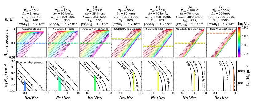
Figure 8: Observed/calculated $R_{{\mathrm{C\text{\sc{i}}}}/{\mathrm{CO}}}$ as a function of CO column density $N_{\mathrm{CO}}$ and [C i/CO] abundance (column density) ratio $N_{\mathrm{C\text{\sc{i}}}}/N_{\mathrm{CO}}$ for 7 representative ISM conditions, based on LTE calculations. Upper panels: Curved lines are $R_{{\mathrm{C\text{\sc{i}}}}/{\mathrm{CO}}}$ versus $N_{\mathrm{C\text{\sc{i}}}}/N_{\mathrm{CO}}$ for different $N_{\mathrm{CO}}$ as indicated by the color. Dashed means CO(2–1) optically thick and $[\mathrm{C}\,{\text{\sc{i}}}]\,(1\textnormal{--}0)$ optically thin, dotted means both are both optically thin, and solid line means both optically thick. Horizontal thick line is the observed $R_{{\mathrm{C\text{\sc{i}}}}/{\mathrm{CO}}}$ value. Lower panels: Black contours are $R_{{\mathrm{C\text{\sc{i}}}}/{\mathrm{CO}}}=0.05,\,0.10,\,0.20$ and $0.50$ in the CO column density versus C i/CO abundance ratio plane. Vertical color shading indicates the final $N_{\mathrm{C\text{\sc{i}}}}/N_{\mathrm{CO}}$ that can match both the observed $R_{{\mathrm{C\text{\sc{i}}}}/{\mathrm{CO}}}{}$ and the assumed $\Sigma_{\mathrm{mol}}$ value noted at the top of each panel.

We determine the LTE solution of [C i/CO] in Fig. 8. To illustrate the complexity of this problem and the degeneracy of the $T_{\mathrm{kin}}$, $N_{\mathrm{CO}}/{\Delta\text{v}}$ and [C i/CO] parameters, we show how $R_{{\mathrm{C\text{\sc{i}}}}/{\mathrm{CO}}}$ ($y$-axis) varies with $N_{\mathrm{C\text{\sc{i}}}}/N_{\mathrm{CO}}$ ($x$-axis) and $N_{\mathrm{CO}}$ (color bar) in the upper panels, and how $R_{{\mathrm{C\text{\sc{i}}}}/{\mathrm{CO}}}$ (contour) can be pinpointed by determining the $\Sigma_{\mathrm{mol}}$ (right $y$-axis). At the top of each column the key parameters of the aforementioned representative ISM conditions are shown as text. The assumed $T_{\mathrm{kin}}$ and ${\Delta\text{v}}$ generally increase from panels (1) to (7) mimicking real conditions. Observational-driven $I_{\mathrm{CO}\,(1\textnormal{--}0)}$ ranges and the assumed $\Sigma_{\mathrm{mol}}$ for these ISM environments are also listed, and can be converted one into the other via $\alpha_{\mathrm{CO}}$. We also list the chosen $\mathrm{[CO/H_{2}]}$ for clarity.

As shown in the upper panels, $R_{{\mathrm{C\text{\sc{i}}}}/{\mathrm{CO}}}$ increases with both $N_{\mathrm{C\text{\sc{i}}}}/N_{\mathrm{CO}}$ and $N_{\mathrm{CO}}$ under low-$T_{\mathrm{kin}}$ conditions. However, a maximum $R_{{\mathrm{C\text{\sc{i}}}}/{\mathrm{CO}}}$ is reached in the high C i column density regime, where an increasing abundance ratio will no longer increase $R_{{\mathrm{C\text{\sc{i}}}}/{\mathrm{CO}}}$. The line ratio saturates at about 0.5 when $T_{\mathrm{kin}}\sim 15$ K, or at about 1 for $T_{\mathrm{kin}}\sim 100$ K. The observed line ratios (horizontal dashed lines) are all lower than the saturation limit of $R_{{\mathrm{C\text{\sc{i}}}}/{\mathrm{CO}}}{}_{\mathrm{max}}\sim 0.7\text{--}0.9$, and corresponds to a range of $N_{\mathrm{CO}}$ or $\Sigma_{\mathrm{mol}}$. This range is very wide in the low-$T_{\mathrm{kin}}$ conditions, with $\log N_{\mathrm{CO}}/\mathrm{cm^{-2}}\sim 17-19$, but is very narrow at $T_{\mathrm{kin}}\sim 100$ K, that is, $R_{{\mathrm{C\text{\sc{i}}}}/{\mathrm{CO}}}$ can be determined from [C i/CO] without much dependence on $N_{\mathrm{CO}}$.

In the lower panels, the contours of $R_{{\mathrm{C\text{\sc{i}}}}/{\mathrm{CO}}}=0.05$, 0.1, 0.2 and 0.5 are shown in the plane of CO column density $N_{\mathrm{CO}}$ versus C i/CO abundance ratio. For a fixed $R_{{\mathrm{C\text{\sc{i}}}}/{\mathrm{CO}}}{}$, a higher $N_{\mathrm{C\text{\sc{i}}}}/N_{\mathrm{CO}}$ corresponds to a lower $N_{\mathrm{CO}}$ in the low-$T_{\mathrm{kin}}$ regime, but $R_{{\mathrm{C\text{\sc{i}}}}/{\mathrm{CO}}}$ becomes insensitive to $N_{\mathrm{CO}}$ at a high $T_{\mathrm{kin}}$. In the latter case, $N_{\mathrm{C\text{\sc{i}}}}/N_{\mathrm{CO}}$ alone determines $R_{{\mathrm{C\text{\sc{i}}}}/{\mathrm{CO}}}{}$. By matching to the expected $\Sigma_{\mathrm{mol}}$ for each ISM condition, we can obtain an unambiguous $N_{\mathrm{C\text{\sc{i}}}}/N_{\mathrm{CO}}$ from the observed $R_{{\mathrm{C\text{\sc{i}}}}/{\mathrm{CO}}}$ as shown in Fig. 8.

In this way, we determine the $N_{\mathrm{C\text{\sc{i}}}}/N_{\mathrm{CO}}$ to be around 0.1–0.2 for conditions (1) and (2), and $\sim 0.4$ for conditions (3) and (5). The SB disk (condition 4) and AGN environments (conditions 6/7) have $N_{\mathrm{C\text{\sc{i}}}}/N_{\mathrm{CO}}\sim 2$ and $\sim 1\text{--}10$, respectively.

The strongly enhanced C i/CO abundance ratios in SB disk and AGN environments are clear signatures of CRDR and XDR, respectively. The NGC 4321 centre is a low-ionization nuclear emission-line region (LINER, e.g., García-Burillo et al. 2005), and given our assumptions it requires $N_{\mathrm{C\text{\sc{i}}}}/N_{\mathrm{CO}}\sim 0.4$ in order to explain the observed low line ratio. The gradually increasing C i/CO abundance ratios in the nuclei of NGC 4321, NGC 3627, NGC 1808 and NGC 7469 agree well with the increasing power of AGN activities, e.g., their X-ray luminosities (Table 1).

Our assumptions for the Galactic cloud ISM condition are mainly based on Heyer et al. (2009), Heyer & Dame (2015) and Roman-Duval et al. (2010). The obtained [C i/CO] $\sim 0.1$ also agrees well with previous studies using C i and CO isotopologues (see Sect. 1. For example, Ikeda et al. (1999) reported $N_{\mathrm{C\text{\sc{i}}}}/N_{\mathrm{CO}}\sim 0.05\textnormal{--}0.2$ for the Orion cloud; Oka et al. (2001) found $N_{\mathrm{C\text{\sc{i}}}}/N_{\mathrm{CO}}=0.064\pm 0.035$ but a peak of $N_{\mathrm{C\text{\sc{i}}}}/N_{\mathrm{CO}}\sim 0.15$ in the DR 15 H ii region and two IR dark clouds; Kramer et al. (2004) found $N_{\mathrm{C\text{\sc{i}}}}/N_{\mathrm{CO}}\sim 0.11\textnormal{--}0.12$ in the massive SF region W3; Genzel et al. (1988) found $N_{\mathrm{C\text{\sc{i}}}}/N_{\mathrm{CO}}\sim 0.2$ for the massive SF region W51; Zmuidzinas et al. (1988) reported $N_{\mathrm{C\text{\sc{i}}}}/N_{\mathrm{CO}}\sim 0.05\textnormal{--}0.15$ in several dense clouds. Recently, Izumi et al. (2021) derived an overall $N_{\mathrm{C\text{\sc{i}}}}/N_{\mathrm{CO}}\sim 0.1$ in the massive SF region RCW38 at $A_{V}\sim 10\textnormal{--}100$, consistent with the Orion cloud, but also saw high [C i/CO] $\sim 0.2\textnormal{--}0.6$ in some even lower column density regions.

Accurate determination of all the ISM properties instead of simple assumptions as in this work requires comprehensive, multi-$J$ CO isotopologue observations (e.g., Teng et al. 2022). Our representative ISM conditions only provide a qualitative diagnostic to understand how to infer the C i/CO abundance ratio from the observed $R_{{\mathrm{C\text{\sc{i}}}}/{\mathrm{CO}}}$ quantity. Their properties may not be very accurate, and are subject to change with future multi-tracer/CO isotopologue studies.

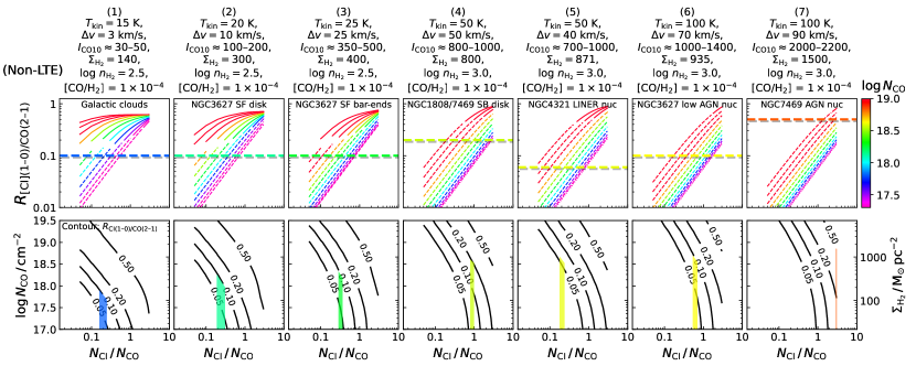
Figure 9: Similar to Fig. 8 but with non-LTE calculations. See Fig. 8 caption for the details.

4.2 Non-LTE results

We perform the non-LTE calculations using the RADEX code (van der Tak et al. 2007) with the Large Velocity Gradient (LVG; i.e., expanding sphere) escape probability (Scoville & Solomon 1974; Goldreich & Kwan 1974). Comparing to LTE, the volume density of H₂ is now an additional property that plays a role. The excitation temperature of each line no longer equals $T_{\mathrm{kin}}$. We compute the non-LTE line ratios in a grid of $(T_{\mathrm{kin}},\,{\Delta\text{v}},\,\mathrm{[CO/H_{2}]},\,N_{\mathrm{C\text{\sc{i}}}}/N_{\mathrm{CO}},\,N_{\mathrm{CO}},\,n_{\mathrm{H_{2}}})$ parameter sets, then study the line and abundance ratios similarly as in the previous section.

In Fig. 9 we show the non-LTE version of Fig. 8. The non-LTE result does not qualitatively differ from that of LTE. The most obvious difference is that at high temperature ($T_{\mathrm{kin}}>50$ K, given our other assumed conditions), the required [C i/CO] is lower by $\times 2$ for the same observed $R_{{\mathrm{C\text{\sc{i}}}}/{\mathrm{CO}}}$, whereas at low temperature ($T_{\mathrm{kin}}\sim 15$ K) a $\lesssim 2\times$ [C i/CO] is expected for the observed line ratio.

As listed in the title of each panel, we assume $\log n_{\mathrm{H_{2}}}/\mathrm{cm^{-3}}=2.5$ to 3.0 for our conditions (1) to (7). This is based on the fact that low-$J$ CO and C i trace the bulk of molecular gas with $\log n_{\mathrm{H_{2}}}/\mathrm{cm^{-3}}\sim 2$–3 (e.g., Leroy et al. 2017; Liu et al. 2021), with a typical value $n_{\mathrm{H_{2}}}\sim 300\,\mathrm{cm^{-3}}$ widely adopted/found for Galactic and nearby galaxy GMCs (e.g., Koda et al. 2012; Pety et al. 2017, see also simulations of Glover & Clark 2012), whereas a smaller portion of their emission is from the dense gas with $\log n_{\mathrm{H_{2}}}/\mathrm{cm^{-3}}\sim 4$–6 (e.g., Gao & Solomon 2004a). The fraction of the dense gas is expected to increase in more starbursting environment (Gao & Solomon 2004b), so does the mean gas density (Liu et al. 2021). Therefore, a $\log n_{\mathrm{H_{2}}}/\mathrm{cm^{-3}}$ of 3.0 is perhaps a reasonable assumption, or at least a lower limit for our galaxy centres. A $10\times$ higher density does not qualitatively change Fig. 9 except for shifting the expected $N_{\mathrm{C\text{\sc{i}}}}/N_{\mathrm{CO}}$ to be 50% higher in the $T_{\mathrm{kin}}>50$ K conditions (making Fig. 9 more like Fig. 8).

Therefore, our non-LTE result strongly confirms the LTE result in the previous section, that the intrinsic C i/CO abundance has to vary significantly from about 0.1–0.2 to about 1–3, in order to explain the observed line ratios from Galactic GMCs (hundred pc scales) and NGC 3627/4321 SF disk GMCs to NGC 1808/7469 SB disk/AGN ($r\lesssim 250$ pc) environments.

5 Discussion

From this study we see that the line ratio $R_{{\mathrm{C\text{\sc{i}}}}/{\mathrm{CO}}}$ increases from 0.1 to 0.2 and $>0.5$ from the SF disk to the SB disk and the vicinity (few hundred pc) of X-ray luminous AGN. Although we may be limited by our sample, we suggest that this trend can be extended to general cases at both local and high redshift, because the C i/CO abundance ratio enhancement is well-predicted by the CRDR and XDR theories.

Papadopoulos (2010) and Papadopoulos et al. (2011) pointed out the key role of CRDR in local (U)LIRGs. With UV photons alone, cold gas in starbursting environments can still be well shielded, hence as cold as $\sim 10$ K. However, with CRs produced from O, B star clusters and supernova remnants, the gas can be uniformly illuminated and heated up. The extremely starbursty local ULIRGs have a CR density ($\xi_{\mathrm{CR}}$) $10^{3}$–$10^{4}$ times that of the Milky Way (Papadopoulos 2010), and thus will naturally dissociate more CO into C i. Bisbas et al. (2017) and Papadopoulos et al. (2018) conducted simulations of molecular gas at tens of pc scale with varying CR strength, and found that when $\xi_{\mathrm{CR}}$ is $\sim 1\textnormal{--}100\,\times$ Galactic value, the gas temperature in the dense gas remains largely unaffected ($\sim 10$ K). However, when $\xi_{\mathrm{CR}}$ reaches $\sim 1000\,\times$ Galactic value as in (U)LIRGs, the gas temperature increases to 30–50 K. The Bisbas et al. (2017) simulation also shows that the C i and C ii fractional abundances at $\log A_{V}\sim 0.5$ increase by one and three orders of magnitude, respectively, and the CO fractional abundance decreases correspondingly by over two orders of magnitude, with an increasing $\xi_{\mathrm{CR}}$ from the Galactic value to $100\,\times$ of that. These results are in line with our calculations in Sect. 4.1.

Meanwhile, the AGN-driven XDR chemistry and molecule/atom excitation have been firstly modeled in great detail by Maloney et al. (1996), Meijerink & Spaans (2005) and Meijerink et al. (2007). In XDRs, photo-ionization becomes the dominant heating source instead of photo-electric emission from dust grains in PDRs, thus more molecules are dissociated and/or ionized. Meijerink & Spaans (2005)’s Model 1 shows that CO molecules are fully dissociated when $N_{\mathrm{H}}<10^{23}\,\mathrm{cm^{-2}}$, then the fractional abundance is gradually increased by six orders of magnitudes from $N_{\mathrm{H}}=10^{23}\,\mathrm{cm^{-2}}$ to $10^{24}\,\mathrm{cm^{-2}}$. By contrast, the C i and C ii abundances are about constant until reaching the densest part ($N_{\mathrm{H}}>10^{24.5}\,\mathrm{cm^{-2}}$). Unlike in PDRs, there is no clear C ii/C i/CO stratification in XDRs (Meijerink et al. 2007; Wolfire et al. 2022). Their Model 2 with a $100\times$ higher energy deposition rate shows that the CO distribution contracts to the highest gas density spots, and the total cumulative [C i/CO] is increased by about 0.2 dex, reaching $N_{\mathrm{C\text{\sc{i}}}}/N_{\mathrm{CO}}\sim 1.6$. This value agrees well with our calculations shown in Figs. 8 and 9 (the ISM condition 7).

Therefore, both in theoretical and observational views, it is clear that the $R_{{\mathrm{C\text{\sc{i}}}}/{\mathrm{CO}}}$ line ratio is a good indicator of the starburst’s CRDR and AGN’s XDR. If a $R_{{\mathrm{C\text{\sc{i}}}}/{\mathrm{CO}}}$ line ratio (to be specific, $I_{[\mathrm{C}\,{\text{\sc{i}}}]\,(1\textnormal{--}0)}/I_{\mathrm{CO}\,(2\textnormal{--}1)}$) reaches 0.2–0.5, then the CRDR plays a crucial role and the abundance ratio [C i/CO] could be $\sim 1$. If it exceeds 0.5–1.0, then it may only be enhanced by an XDR, e.g., caused by an X-ray luminous AGN, which boosts the abundance ratio [C i/CO] to $\gtrsim 1$–2.

6 Conclusion

We presented new beam- and $uv$-coverage-matched $[\mathrm{C}\,{\text{\sc{i}}}]\,(1\textnormal{--}0)$ and CO(2–1) maps in the galactocentric radius $r\lesssim 7$ kpc SF disk of NGC 3627 at $\sim 190$ pc resolution, and in the $r\lesssim 3$ kpc disk of NGC 4321 at $\sim 270$ pc resolution. They are among the largest C i mosaic mappings available in nearby galaxies.

We combined the imaging of $[\mathrm{C}\,{\text{\sc{i}}}]\,(1\textnormal{--}0)$ and CO(2–1) in two nearby, more starbursty and AGN-hosting galaxies, i.e., NGC 1808 central $\sim 1$ kpc, and NGC 7469 central $\sim 1.5$ kpc at 140–160 pc resolutions. Together, we studied the spatial distributions of C i and CO, and their line ratio $R_{{\mathrm{C\text{\sc{i}}}}/{\mathrm{CO}}}$ as functions of various galaxy resolved properties, including CO brightness (Fig. 4), ISRF $\left<U\right>$ (Fig. 6), and metallicity (Fig. 7).

In order to obtain the underlying intrinsic [C i/CO] abundance ratio from the observed line ratio $R_{{\mathrm{C\text{\sc{i}}}}/{\mathrm{CO}}}$, we assumed 7 representative ISM conditions and did both LTE and non-LTE calculations.

We summarize our findings as below:

• The majority of the molecular gas in the SF disks of NGC 3627 and NGC 4321 has a uniform ${R}_{\mathrm{C{\text{\sc{i}}}{10}}/\mathrm{CO{21}}}=0.10\pm 0.05$. $[\mathrm{C}\,{\text{\sc{i}}}]\,(1\textnormal{--}0)$ and $\mathrm{CO}\,(2\textnormal{--}1)$ exhibit very similar spatial distributions at our 140–270 pc resolution.

• The majority of the molecular gas in the SB disk of NGC 1808 has ${R}_{\mathrm{C{\text{\sc{i}}}{10}}/\mathrm{CO{21}}}=0.20\pm 0.05$. This elevated line ratio compared to the SF disk is likely caused by a $\sim 3\text{--}5\times$ increased [C i/CO] abundance ratio, based on our LTE and non-LTE calculations and parameter assumptions (Figs. 8 and 9).

• The centres ($r\lesssim 250$ pc) of NGC 4321, NGC 3627, NGC 1808 and NGC 7469 show a strongly increasing trend in ${R}_{\mathrm{C{\text{\sc{i}}}{10}}/\mathrm{CO{21}}}$, from 0.05 to 0.5, as a function of $I_{\mathrm{CO}\,(2\textnormal{--}1)}$ — i.e., ${R}_{\mathrm{C{\text{\sc{i}}}{10}}/\mathrm{CO{21}}}\approx 0.035\,(I_{\mathrm{CO}\,(2\textnormal{--}1)}/[100\;\mathrm{K\,km\,s^{-1}}])^{0.8}$. The inferred [C i/CO] abundance ratio from our non-LTE calculation changes from $\sim 0.2$ to $\sim 3$, in line with the increasing X-ray luminosity of the centres/AGNs.

• The observed $R_{{\mathrm{C\text{\sc{i}}}}/{\mathrm{CO}}}$ versus ISRF trend is fairly flat, i.e., $R_{{\mathrm{C\text{\sc{i}}}}/{\mathrm{CO}}}$ is insensitive to ISRF intensity changes, similar to the PDR model prediction calculated with PDRToolbox (although our resolution is much coarser than the physical scale of PDR models; Sect. 3.3).

• We find a $R_{{\mathrm{C\text{\sc{i}}}}/{\mathrm{CO}}}$ versus metallicity trend consistent with previous observations that covered lower-metallicity environments ($\sim 0.2\,\mathrm{Z_{\odot}}$; Bolatto et al. 2000b), within the metallicity range ($\sim 0.7\text{--}1\,\mathrm{Z_{\odot}}$) of our sample (Sect. 3.4).

• Our inferred [C i/CO] abundance ratios agree well with the CRDR and XDR’s theoretical studies. Given the drastically changed $R_{{\mathrm{C\text{\sc{i}}}}/{\mathrm{CO}}}$, we propose that the C i to CO line ratio can be a promising indicator of CRDR (starbursting) and XDR (AGN). For instance, an observed line flux ratio of ${R}_{\mathrm{C{\text{\sc{i}}}{10}}/\mathrm{CO{21}}}\sim 0.2\textnormal{--}0.5$ and $\gtrsim 0.5$ effectively indicates CRDR and XDR, respectively.

• We do not find ubiquitous “CO-dark”, C i-bright gas at the outer $r\sim 1\text{--}3$ kpc disks of NGC 3627 and NGC4321, nor systematic enhancement in $R_{{\mathrm{C\text{\sc{i}}}}/{\mathrm{CO}}}$ at CO-faintest sightlines via stacking, mainly due to the incompleteness of our data. Nevertheless, a few sightlines, e.g., Region 22 in NGC 3627 show high $R_{{\mathrm{C\text{\sc{i}}}}/{\mathrm{CO}}}$ $\sim 0.5$ which do not fully comply with the noise behavior seen in our CASA simulations.

Appendix A Data reduction, imaging and moment map generation

After downloading the raw data, i.e., 12m+7m for $\mathrm{CO}\,(2\textnormal{--}1)$ and 7m for $[\mathrm{C}\,{\text{\sc{i}}}]\,(1\textnormal{--}0)$, respectively, we ran the observatory calibration pipeline (“scriptForPI”) to reduce the data. As shown in Leroy et al. (2021a), the observatory calibration produces well-calibrated visibility data without further manual flagging. We then split out the visibility data and proceeded to the imaging step.

In order to match the spatial resolution of $\mathrm{CO}\,(2\textnormal{--}1)$ and $[\mathrm{C}\,{\text{\sc{i}}}]\,(1\textnormal{--}0)$, we carefully matched their $uv$ ranges. We flagged the $\mathrm{CO}\,(2\textnormal{--}1)$ visibility data outside the $uv$ range of 19–68 m ($\sim$15–52k$\lambda$) so as to match the $uv$ range of the $[\mathrm{C}\,{\text{\sc{i}}}]\,(1\textnormal{--}0)$ data (minimum to 80% percentile: 8.9–32 m, or $\sim$15–52k$\lambda$). Given that the $[\mathrm{C}\,{\text{\sc{i}}}]\,(1\textnormal{--}0)$ $uv$ plane distribution is elliptic, while the $uv$ range selection in CASA is circular, our chosen thresholds are adjusted to make the final $\mathrm{CO}\,(2\textnormal{--}1)$ synthesized beam similar to that of $[\mathrm{C}\,{\text{\sc{i}}}]\,(1\textnormal{--}0)$. Note that in a later step we also convolved both image cubes to the exact same rounded beam ($3.46^{\prime\prime}$) before generating the moment maps.

The PHANGS-ALMA imaging & post-processing pipeline  developed by Leroy et al. (2021a) is used for creating line cubes and moment maps. The code is suitable for general nearby galaxy strong line mapping interferometric and total power mosaic data. In brief, the visibility data are carefully transformed into the user-given channel width and frequency range corresponding to the line plus line-free channels, then continuum is subtracted by fitting an order of zero polynomial. Then, two stages of imaging (“cleaning”) are performed: first a multi-scale cleaning down to $\sim 4\sigma$, then a single-scale cleaning down to $\sim 1\sigma$. At each stage, CASA’s tclean task is iteratively called so as to force many major cycles, which has proven to improve the accuracy of the deconvolution. Before and during the second stage cleaning, a clean mask is computed at each iteration according to the outcome of previous iteration by finding all $>2\sigma$ pixels associated with $>4\sigma$ peaks in a watershed algorithm (Rosolowsky & Leroy 2006; Rosolowsky et al. 2021). In this way the cleaning can include as much signal as possible and ensure a signal-free residual.

Then the image cubes are corrected for the primary beam attenuation, converted to Kelvin units, and convolved to a common beam, which is the coarser beam of $\mathrm{CO}\,(2\textnormal{--}1)$ and $[\mathrm{C}\,{\text{\sc{i}}}]\,(1\textnormal{--}0)$. Because of our $uv$ range flagging before imaging, the directly tclean-imaged beam sizes are already close. This convolution further precisely matches $\mathrm{CO}\,(2\textnormal{--}1)$ and $[\mathrm{C}\,{\text{\sc{i}}}]\,(1\textnormal{--}0)$ image cube beams.

Next, moment maps are generated with modules in the PHANGS-ALMA pipeline, consistently for CO and C i. This process includes firstly constructing noise and mask cubes from the image cubes, then combining the masks (i.e., where science signal should present), then computing moment 0 – line integrated intensity, moment 1 – line peak velocity, and moment 2 – line width. The mask cubes are the key in producing moment maps. Here two masks are built: a “broad mask” which contains as much plausible science signal as possible, and a “strict mask” which is optimized for high-confidence signal. The strict mask is made by finding peaks that have $>4\sigma$ over two consecutive channels then expanding down to $2\sigma$ also with the watershed algorithm. Then the broad mask is obtained by aggregating strict masks made from image cubes convolved to coarser resolutions ($\sim 30^{\prime\prime}$ in this work as well as in Leroy et al. 2021a). To make consistent moment maps for CO and C i, we aggregate their masks together as a joint mask, for broad and strict masks, respectively, then their final moment maps are computed within the joint mask.

The resulting $\mathrm{CO}\,(2\textnormal{--}1)$ and $[\mathrm{C}\,{\text{\sc{i}}}]\,(1\textnormal{--}0)$ line intensity maps are then used for our next line ratio analysis. The line velocity and line width maps are not further analyzed, but are consistent with the products from the PHANGS-ALMA survey’s data release as well as in Lang et al. (2020). Given that the PHANGS-ALMA 12m+7m+tp $\mathrm{CO}\,(2\textnormal{--}1)$ has the full spatial information and are deeper, their line velocity and line width maps are more useful for kinematic studies than ours produced from this work.

Appendix B Assessing the missing flux in the NGC 3627 C i data

We assess the level of missing flux in the NGC 3627 C i data in three ways: (a) comparing with the Herschel SPIRE FTS $[\mathrm{C}\,{\text{\sc{i}}}]\,(1\textnormal{--}0)$ observation in this galaxy, (b) comparing the $uv$-trimmed CO(2-1) moment-0 map with the PHANGS-ALMA short-spacing corrected (12m+7m+tp) moment-0 map, and (c) performing CASA simulation and comparing with the “true” moment-0 from the skymodel and the derived product from the simulated visibilities.

Method (a): NGC 3627 has been observed with the Herschel SPIRE (Griffin et al. 2010) Fourier Transform Spectrometer (FTS; Naylor et al. 2010) in mapping mode with nearly Nyquist sampling. Liu et al. (2015) reduced the archival data and extracted the line fluxes for each groups of pointings. $[\mathrm{C}\,{\text{\sc{i}}}]\,(1\textnormal{--}0)$ is detected with $\mathrm{S/N}\sim 4-5$ at three sightlines from the galaxy centre to the southern bar end, with R.A. and Dec. coordinates (J2000) 170.061905, +12.991336, 170.066361 +12.987091, and 170.071243 +12.981615, respectively. The $[\mathrm{C}\,{\text{\sc{i}}}]\,(1\textnormal{--}0)$ luminosities are $1.44\pm 0.31$, $2.01\pm 0.48$, and $1.71\pm 0.40\times 10^{7}\;\mathrm{K\,km\,s^{-1}\,pc^{2}}$, respectively, where the errors are purely from the RMS of line-free FTS spectra. By convolving our $[\mathrm{C}\,{\text{\sc{i}}}]\,(1\textnormal{--}0)$ line cube to the FTS beam of $\sim 39^{\prime\prime}$ then extracting the moment maps, we measure a $[\mathrm{C}\,{\text{\sc{i}}}]\,(1\textnormal{--}0)$ line luminosity of $0.52$, $0.33$ and $0.29\times 10^{7}\;\mathrm{K\,km\,s^{-1}\,pc^{2}}$ at the above three positions, respectively, which means a missing flux of $36-75\%$ at the galaxy centre and $68-88\%$ at the southern bar end (at a 95% confidence level).

Method (b): We made ratio maps of our $uv$-trimmed CO(2-1) moment-0 map, and that of the original PHANGS-ALMA short-spacing-corrected (12m+7m+tp) CO(2-1) data but convolved to the corresponding resolution before making the moment maps. The ratio maps are made at two resolutions: the FTS $39^{\prime\prime}$ beam, and our working resolution of $3.46^{\prime\prime}$. The former leads to a missing flux of 26%, 31% and 36% from the galaxy centre to the southern bar end. Note that the above Herschel FTS analysis indicates in general a higher missing flux, but the FTS measurements are of low $\mathrm{S/N}$ and errors purely from the RMS of the spectra can not fully account for other errors like pointing, spectral response, off-axis spaxel calibration, etc. The latter ratio map shows that the missing flux at our working resolution and within the strict mask varies from $\sim$60% to as low as 6% at the brightest pixels. This is consistent with our next method based on simulation.

Method (c): We performed detailed simulations of 7m-only $[\mathrm{C}\,{\text{\sc{i}}}]\,(1\textnormal{--}0)$ and 12m+7m $\mathrm{CO}\,(2\textnormal{--}1)$ observations with the CASA simobserve task. We use the PHANGS-ALMA 12m+7m CO(2-1) clean model cube (one of the output products of CASA tclean runs) as the input skymodel for $\mathrm{CO}\,(2\textnormal{--}1)$, and that scaled by a factor of 0.2 in Kelvin units for $[\mathrm{C}\,{\text{\sc{i}}}]\,(1\textnormal{--}0)$ (representing a constant $R_{{\mathrm{C\text{\sc{i}}}}/{\mathrm{CO}}}=0.2$). Note that we do not use the short-spacing-corrected PHANGS-ALMA CO(2-1) cube because it has a finite beam size of $\sim 1^{\prime\prime}$, and simulation based on that may result in more extended emissions. On the contrary, the clean model cube has an infinite resolution, and because both “multiscale” and “singlescale” cleaning are used in the PHANGS-ALMA imaging, the clean model contains point as well as extended sources. We also set the actual observing dates and integration times as the real observations. Then we run CASA simobserve to simulate the visibilities of each observing block, concatenate them together, and process them into image cubes and moment maps in the same way as described in Appendix A. Meanwhile, by convolving the input skymodel with a 2D Gaussian beam corresponding to our working resolution, and integrating over the spectral axis, we obtain a “true” skymodel moment-0 map which can be directly compared to the imaged moment-0 maps from the simulation. Their ratio map shows a missing flux of $\sim 50\%$ to $\sim 7\%$ in the strict mask, and more specifically, 24%, 58%, 85% and 96% pixels selected in our method as for real data have a missing flux $<20\%$, $<30\%$, $<40\%$ and $<50\%$, respectively.

Fig. 10 illustrates the results from methods (b) (upper panels) and (c) (lower panels). Left panels show the $\mathrm{CO}\,(2\textnormal{--}1)$ moment-0 maps, analyzed at the same working resolution as our main analysis in Appendix A. The simulated data show a fainter emission because we used the clean mode cube as the skymodel, which was made by cleaning the PHANGS-ALMA 12m+7m data down to 1 $\sigma$ within the clean mask voxels. This will indeed lose some fluxes. However, the right panels show that the two methods lead to consistent missing flux results.

Note that in the last panel of Fig. 10, some regions appear black in the simulation-based analysis because we require line ratios to be analyzed in the strict mask, while these regions are not in it anymore. This is because the skymodel loses some fluxes as mentioned above, thus the strict mask is smaller, and also because in the simulation we assumed a constant $R_{{\mathrm{C\text{\sc{i}}}}/{\mathrm{CO}}}$ which may lead to fainter C i than real data along faint sightlines, e.g., Region 22, thus further shrinking the strict mask where both lines need to have sufficient $\mathrm{S/N}$.

Bearing these in mind, we conclude that methods (b) and (c) have consistent results on the missing flux, and method (a) is less accurate due to the unconsidered uncertainties.

These checks show that the overall missing flux in NGC 3627 is 31% based on the full- and trimmed-$uv$ $\mathrm{CO}\,(2\textnormal{--}1)$ analysis, or $\sim 36-88\%$ based on the more-uncertain Herschel data. At the pixel level, it varies from 7% to $\sim$50% from bright to faint sightlines at our working resolution of $3.46^{\prime\prime}$. These values are as expected given our ACA-only observation setup. We emphasize again that by applying the $uv$-matching in our data reduction, our C i/CO line ratio study is not obviously affected by the missing flux issue, except perhaps in the faintest pixels or “cloud edges”.

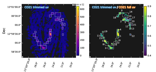
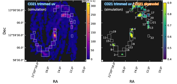
Figure 10: Upper left panel: short-spacing corrected (12m+7m+tp) PHANGS-ALMA CO(2-1) derived moment-0 map. Upper right panel: ratio map of the $uv$-trimmed CO(2-1) moment-0 map used in this work to that in the left panel. Lower left panel: the CO(2-1) moment-0 map derived from our simulation with $uv$ trimming as for real data. Lower right panel: ratio map of the $uv$-trimmed CO(2-1) moment-0 map based on the simulation to the “true” skymodel moment-0 map as shown left. All moment maps are derived by first convolving cubes to our working resolution of $3.46^{\prime\prime}$ then performing masking analysis as described in Appendix A, except for the “true” skymodel moment-0 map which is computed without any masking. Note that in the simulation based analysis, some regions have too low $\mathrm{S/N}$ due to their faint CO brightness or insufficient cleaning, thus they are out of the mask and show blank line ratios (instead of very low missing flux) in the lower right panel.

Appendix C Assessing noise-induced C i enhancement with simulation

In Appendix B we described our simulation. We also use it to assess how the noise can induce artificial [C i/CO] line ratio variation.

In Fig. 11 we show the line ratio map from the simulation with a constant $R_{{\mathrm{C\text{\sc{i}}}}/{\mathrm{CO}}}=0.2$, and in Fig. 12 we show the scatter plots with simulation results similar to Fig. 4. Interestingly, we see certain C i/CO variations, especially C i “enhancement” at the edge of galaxy centre’s gas clump (region 1), and the edge of the northern spiral arm (Region 14). Nevertheless, the trend is very different from the real data, i.e., Fig. 4. First, galaxy centre has a much weaker [C i/CO] in the real data, whereas in the simulation it is inverted. Second, the scatter is much larger in real data, with a tail of C i enhanced regions which is not seen in the simulation. Third, from the bottom panels of Fig. 12, where $\mathrm{S/N}$ is shown, we see that $R_{{\mathrm{C\text{\sc{i}}}}/{\mathrm{CO}}}$ is biased to be lower in low-$\mathrm{S/N}$ situation. Thus the high C i in real data is unlikely to be a bias of low $\mathrm{S/N}$.

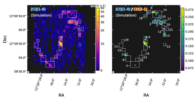
Figure 11: C i line flux and $R_{{\mathrm{C\text{\sc{i}}}}/{\mathrm{CO}}}$ line ratio image from the simulation mimicking real observation but with a constant input line ratio $R_{{\mathrm{C\text{\sc{i}}}}/{\mathrm{CO}}}=0.2$.

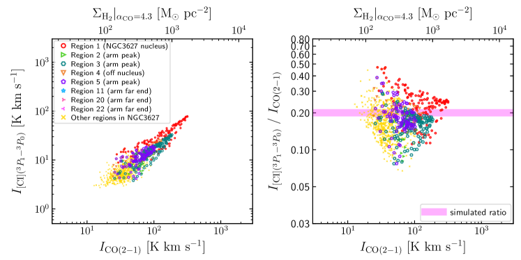
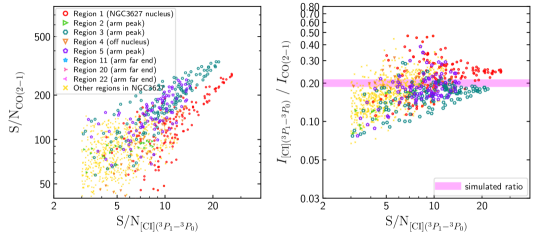
Figure 12: Upper panels: $[\mathrm{C}\,{\text{\sc{i}}}]\,(1\textnormal{--}0)$ and $\mathrm{CO}\,(2\textnormal{--}1)$ line brightness and ratio similar to Fig.4 but from our simulation (with a constant input $R_{{\mathrm{C\text{\sc{i}}}}/{\mathrm{CO}}}=0.2$ as indicated by the horizontal shading in the right panels). Lower panels: Similar to the upper panels but showing line $\mathrm{S/N}$ instead of brightness. This illustrates how $R_{{\mathrm{C\text{\sc{i}}}}/{\mathrm{CO}}}$ can be biased in low-$\mathrm{S/N}$ situation.

Appendix D C i and CO spectra of selected regions in NGC 3627

We show the examples of $[\mathrm{C}\,{\text{\sc{i}}}]\,(1\textnormal{--}0)$ and $\mathrm{CO}\,(2\textnormal{--}1)$ moment-0 maps and spectra for Regions 1, 4 & 22 in Fig. 13. They represent the NGC 3627 centre, off-centre location and the location at the outer disk of the gaseous spiral arm as discussed in Sect. 3.

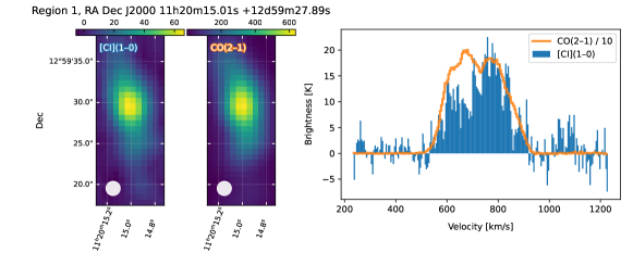
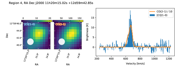
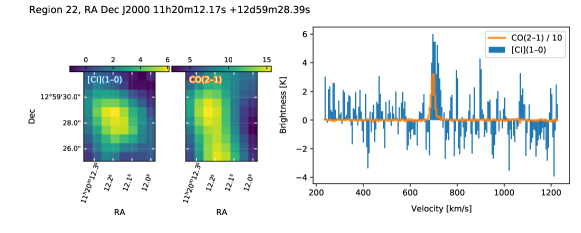
Figure 13: $[\mathrm{C}\,{\text{\sc{i}}}]\,(1\textnormal{--}0)$ and $\mathrm{CO}\,(2\textnormal{--}1)$ moment-0 maps and spectra of Regions 1, 4 and 22 as defined in Fig. 1. All regions’ spectra are available in our online data release (see Sect. 2.2).