Single-step first order phase transition and gravitational waves in a SIMP dark matter scenario

Abstract

We investigate the non-zero temperature dynamics of a sub-GeV dark matter scenario freezing-out via self-interactions. As a prototype, we take up the case of a scalar dark matter species undergoing $3\to 2$ number changing annihilations catalysed by another scalar. We study the shape of the thermal potential of this scenario in a parameter region accounting for the observed relic abundance. An analysis reveals the possibility of a first order phase transition with bubble nucleation occurring at sub-GeV temperatures. This finding can be correlated with the typical sub-GeV masses in the framework. The gravitational wave spectra associated with such a phase transition is subsequently computed.

I Introduction

It has been concurred by numerous observations Rubin:1970zza ; Bertone:2004pz ; Hu:2001bc ; WMAP:2012nax that around a fourth of the total energy budget of the universe is some non-luminous matter known as dark matter (DM). The amount of such matter in the universe is also well measured from various observations, e.g., cosmic microwave background (CMB) Planck:2018vyg and large scale structure surveys Blumenthal:1984bp . If DM is thought to be an elementary particle, then there is no information available from the current experiments on its mass and quantum numbers. More importantly, that there is no such particle candidate for DM within the Standard Model (SM), advocates the presence of additional dynamics. While DM can be hypothesized to stem from some beyond-the-Standard Model (BSM) framework, a possibility in this direction is that DM is a weakly interacting massive particle (WIMP) Kolb:1990vq ; Jungman:1995df ; Bertone:2004pz ; Feng:2010gw ; Arcadi:2017kky ; Roszkowski:2017nbc . That is, the DM-SM interactions are in the weak ballpark. Moreover, the DM relic abundance in the WIMP paradigm is generated typically through $2_{\text{DM}}\to 2_{\text{SM}}$ annihilation processes followed by a thermal freeze out.

Search for DM through its scattering with nuclei at terrestrial detectors is known as direct detection XENON:2018voc ; LUX:2017ree . However, non-observation of such scattering at have put stringent upper limits on the corresponding cross sections, and ultimately, on the DM-SM interactions. Such small interactions are also consistent with the null results obtained in DM searches at the energy frontier, the Large Hadron Collider (LHC) being the prime example here Abercrombie:2015wmb . These results have pushed a plethora of WIMP scenarios to a corner Roszkowski:2017nbc ; Arcadi:2017kky . An interesting alternative therefore could a strongly interacting massive particle (SIMP) Bernal:2015xba ; Choi:2016hid ; Choi:2016tkj ; Bernal:2017mqb ; Chauhan:2017eck ; Mohanty:2019drv ; Bhattacharya:2019mmy ; Lee:2015gsa ; Yamanaka:2015tba ; Hochberg:2015vrg ; Hochberg:2014kqa ; Choi:2017zww ; Choi:2018jsb ; Herms:2018ajr ; Ma:2015mjd . In this case, the freeze-out dynamics is driven by DM matter number changing processes, i.e., processes that feature an imbalance of DM particles in the initial and final states. The main advantage of the SIMP paradigm is that it allows such number changing processes to be predominantly driven by DM self interactions. The DM-SM interaction stengths are thus permitted to be appropriately small so as to conform with the limits from direct detection and colliders. A SIMP therefore typically has sub-GeV mass and a large self-scattering cross section.

With the advent of gravitational wave (GW) interferometry Thrane:2013oya ; Sathyaprakash:2012jk ; LISA:2017pwj ; Crowder:2005nr ; Seto:2001qf ; Sato:2017dkf ; Lentati:2015qwp ; Janssen:2014dka ; Fairbairn:2019xog , it has become possible to probe a dark sector through its GW imprints Breitbach:2018ddu ; Schwaller:2015tja ; Jaeckel:2016jlh ; Addazi:2016fbj ; Baldes:2017rcu ; Tsumura:2017knk ; Baldes:2018emh ; Croon:2018erz . In this study, we aim to study the possibility of a strong first order phase transition (SFOPT) Kamionkowski:1993fg ; Witten:1984rs ; Hogan:1986qda ; Grojean:2006bp and the GW spectrum from associated with a sub-GeV SIMP framework. The model we take up is where the SM is extended by the scalars $\phi$ and $\delta$ that are singlets under the SM gauge symmetry Mohanty:2019drv . The scalar $\phi$, stabilised by a governing $\mathbb{Z}_{2}$ symmetry, becomes the DM candidate here. The number changing process for this case that is consistent with the $\mathbb{Z}_{2}$ is $\phi\phi\phi\to\phi h_{2}$, where $h_{2}$ is an admixture of $\delta$ and the Higgs doublet $H$. The scalar $\delta$ and its interaction with the DM $\phi$ thus play crucial roles in generating the observed relic density through the aforesaid $3\to 2$ dynamics. Given the importance of $\delta$ in this setup, a pertinent question to ask is whether the same can trigger a SFOPT and how strong is the resulting GW amplitude. We plan to explore this possibility here by incorporating finite temperature corrections to the scalar potential along the direction of $\delta$.

The study is organised as follows. We introduce the setup and outline the $3\to 2$ dynamics in section II. Thermal corrections to the scalar potential are computed in section III. The same section presents the GW amplitude for representative benchmark points. We finally conclude in section IV. Some important formulae can be found in the Appendix V.

II The sub-GeV dark matter framework and $3\to 2$ dynamics

We extend the SM with the real gauge singlet scalars $\phi$ and $\delta$ Mohanty:2019drv . A $\mathbb{Z}_{2}$ symmetry is imposed under which $\phi\to-\phi$ while all other fields transform trivially. This negative $\mathbb{Z}_{2}$ charge for $\phi$ stabilises the same and makes it a potential DM candidate. The scalar potential of the setup reads

$$V = \frac{\mu_{\phi}^{2}}{2}\phi^{2}+\frac{\mu_{\delta}^{2}}{2}\delta^{2}+\mu_{H}^{2}H^{\dagger}H+\frac{\mu_{21}}{2}\phi^{2}\delta+\frac{\mu_{22}}{3!}\delta^{3}$$ (1)

$$+\mu_{23}H^{\dagger}H\delta+\frac{\lambda_{11}}{4!}\phi^{4}+\frac{\lambda_{12}}{4}\phi^{2}\delta^{2}+\frac{\lambda_{22}}{4!}\delta^{4}$$

$$+\frac{\lambda_{13}}{2}\phi^{2}H^{\dagger}H+\frac{\lambda_{23}}{2}\delta^{2}H^{\dagger}H+\lambda_{33}\left[H^{\dagger}H\right]^{2}.$$

In the above, all parameteres are taken real and $H$ denotes the SM Higgs doublet. The doublet $H$ and the singlet $\delta$ receive vacuum expectation values (VEVs) $v$ and $v_{\delta}$ respectively. One then writes

$$H=\begin{pmatrix}G^{+}\\ \frac{1}{\sqrt{2}}(v+h+iG^{0})\end{pmatrix};~{}~{}~{}\delta=v_{\delta}+\delta^{\prime}.$$ (2)

Here, $v$ = 246 GeV. It is noted that $\phi$ does not receive a VEV and thus the $\mathbb{Z}_{2}$ remains intact. In all, such a configuration of the VEVs introduces a mixing between $h$ and $\delta^{\prime}$. The mixing of $\phi$ is however forbidden by the $\mathbb{Z}_{2}$ symmetry. The mass matrix in the $(h~{}~{}\delta^{\prime})$ basis is

$$\mathcal{M}^{2} = \begin{pmatrix}2\lambda_{33}v^{2}&\lambda_{23}\hskip 1.42262ptvv_{\delta}+\mu_{23}v\\ \lambda_{23}\hskip 1.42262ptvv_{\delta}\hskip 1.42262pt+\mu_{23}v&\frac{\mu_{22}v_{\delta}}{2}+\frac{\lambda_{22}}{3}v_{\delta}^{2}-\frac{\mu_{23}}{2}\frac{v^{2}}{v_{\delta}}\end{pmatrix}.$$ (3)

We have made use of the tadpole conditions $\frac{\partial V}{\partial h}=0=\frac{\partial V}{\partial\delta^{\prime}}$ while deriving Eq.(3). One derives the tadpole conditions to be

$$\mu_{h}^{2} = -\big{(}\mu_{23}\hskip 2.84526ptv_{\delta}+\frac{\lambda_{23}}{2}\hskip 2.84526ptv_{\delta}^{2}+\lambda_{33}\hskip 2.84526ptv^{2}\big{)},$$ (4a)

$$\mu_{\delta}^{2} = -\big{(}\frac{\mu_{22}}{2}v_{\delta}+\frac{\lambda_{22}}{6}v_{\delta}^{2}+\frac{\mu_{23}}{2}\frac{v^{2}}{v_{\delta}}+\frac{\lambda_{23}}{2}v^{2}\big{)}.$$ (4b)

Eq.(3) is diagonalised through a $2\times 2$ rotation parameterised by a mixing angle $\theta$. That is,

$$\begin{pmatrix}h\\ \delta^{\prime}\end{pmatrix}=\begin{pmatrix}\cos\theta&\sin\theta\\ -\sin\theta&\cos\theta\end{pmatrix}\begin{pmatrix}h_{1}\\ h_{2}\end{pmatrix},$$ (5)

which leads to the eigenstates $(h_{1},h_{2})$. We identify $h_{1}$ with the discovered Higgs boson with $m_{h_{1}}$ = 125 GeV. The DM mass is given by

$$m_{\phi}^{2}=\mu^{2}_{\phi}+\mu_{21}v_{\delta}+\frac{1}{2}\lambda_{12}v^{2}_{\delta}+\frac{1}{2}\lambda_{13}v^{2}.$$ (6)

Some of the parameters in the scalar potential can be expressed in terms of the physical quantities of the theory such as masses and mixing angles using the relations

$$\lambda_{33} = \frac{(m_{h_{1}}^{2}\cos^{2}\theta+m_{h_{2}}^{2}\sin^{2}\theta)}{2\hskip 1.42262ptv^{2}},$$ (7a)

$$\mu_{23} = \frac{(m_{h_{2}}^{2}-m_{h_{1}}^{2})\cos\theta\sin\theta}{v}-\lambda_{23}\hskip 1.42262ptv_{\delta},$$ (7b)

$$\mu_{22} = \frac{2}{v_{\delta}}(m_{h_{1}}^{2}\sin^{2}\theta+m_{h_{2}}^{2}\cos^{2}\theta)-\frac{\lambda_{22}}{3}\hskip 1.42262ptv_{\delta}$$ (7c)

$$+\mu_{23}\frac{v^{2}}{v^{2}_{\delta}},$$

$$\mu_{\phi}^{2} = m^{2}_{\phi}-\mu_{21}v_{\delta}-\frac{1}{2}\lambda_{12}v^{2}_{\delta}-\frac{1}{2}\lambda_{13}v^{2}.$$ (7d)

The independent variables of the present framework thus are $\{m_{h_{2}},m_{\phi},\mu_{21},v_{h},v_{\delta},\text{sin}\theta,\lambda_{11},\lambda_{12},\lambda_{13},\lambda_{22},\lambda_{23}\}$.

The relic abundance in a strongly interacting DM setup is generated through number changing processes. In this setup, the leading number changing processes consistent with the $\mathbb{Z}_{2}$ is $\phi\phi\phi\to\phi S$ where $S=h_{1},h_{2}$. We list below the Feynman diagrams for illustration.

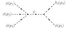
Figure 1: $\phi$-mediated Feynman diagram responsible for annihilation of $\phi$.

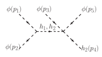
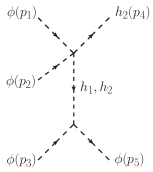
Figure 2: Feynman diagrams show annihilation of $\phi$ mediated by $h_{1}$, $h_{2}$.

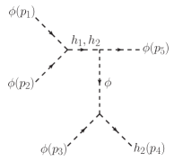
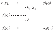
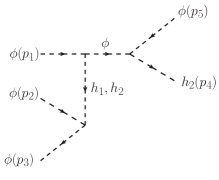
Figure 3: Annihilation diagrams mediated by $h_{1}$, $h_{2}$ and $\phi$.

Figs.1, 2 and 3 show the $3\to 2$ annihilation diagrams. We take the limit where sin$\theta$ and $\lambda_{13}$ are tiny. The tiny sin$\theta$ conforms with the constraints on $\delta-H$ mixing from direct search and Higgs signal strengths. The $\phi-\phi-h_{1}$ trilinear coupling becomes negligibly small in this limit while the $\phi-\phi-h_{2}$ coupling becomes $\simeq(\mu_{21}+\lambda_{12}v_{\delta})$. Moreover, the limit entails that the $\phi$-mediated amplitude in Fig.1 is the dominant one. The following is its expression:

$$\mathcal{M}\simeq\frac{\lambda_{11}(\mu_{21}+\lambda_{12}v_{\delta})}{(p_{1}+p_{2}+p_{3})^{2}-m^{2}_{\phi}}\simeq\frac{\lambda_{11}(\mu_{21}+\lambda_{12}v_{\delta})}{8m_{\phi}^{2}}.$$ (8)

In the last step above, we have neglected the DM velocity, a justifiable assumption for non-relativistic DM. One can approximate $p_{i}\simeq(m_{\phi},\vec{0})$ in that case. The evolution of the DM comoving number density $Y_{\phi}$ is described by the Boltzmann equation Kolb:1990vq

$$\frac{dY_{\phi}}{dx}=-\frac{x~{}s^{2}}{3\mathcal{H}}\langle\sigma v^{2}\rangle_{\phi\phi\phi\rightarrow\phi h_{2}}\Big{(}Y^{3}_{\phi}-Y_{\phi}Y^{\text{eq}}_{\phi}Y^{\text{eq}}_{h_{2}}\Big{)},$$ (9)

where $s=\frac{2\pi^{2}}{45}~{}g_{*s}T^{3}$ is the entropy density and the Hubble parameter is $\mathcal{H}=\sqrt{\frac{8\pi^{3}Gg_{*}T^{4}}{90}}$. Besides, $Y^{\text{eq}}_{P}$ denotes the equilibrium comoving number density of a particle $P$ and $\langle\sigma v^{2}\rangle_{\phi\phi\phi\rightarrow\phi h_{2}}$ is the thermally averaged $3\to 2$ cross section Pierre:2018man . It can be related to $\sigma v^{2}_{\phi\phi\phi\rightarrow\phi h_{2}}$ using modified Bessel functions $K_{n}(x)$ as

$$\braket{\sigma v^{2}}_{\phi\phi\phi\to\phi h_{2}}(T) = \Bigg{(}\frac{K_{1}\big{(}\frac{m_{\phi}}{T}\big{)}}{K_{2}\big{(}\frac{m_{\phi}}{T}\big{)}}\Bigg{)}^{3}(\sigma v^{2})_{\phi\phi\phi\to\phi h_{2}},\text{with}$$

$$(\sigma v^{2})_{\phi\phi\phi\to\phi h_{2}} = \frac{|\mathcal{M}|^{2}}{72\pi m^{3}_{\phi}}$$

$$\times \sqrt{\bigg{(}1-\frac{5}{16}\Big{(}\frac{m_{h_{2}}}{m_{\phi}}\Big{)}^{2}+\frac{1}{64}\Big{(}\frac{m_{h_{2}}}{m_{\phi}}\Big{)}^{4}\bigg{)}}.$$ (10)

Further, Eq.(9) becomes the following upon taking $g_{*s}\simeq g_{*}$.

$$\frac{dY_{\phi}}{dx} = -0.116~{}g^{3/2}_{*}~{}M_{\text{Pl}}\frac{m^{4}_{\phi}}{x^{5}}~{}\langle\sigma v^{2}\rangle_{\phi\phi\phi\rightarrow\phi h_{2}}$$ (11)

$$~{}~{}~{}~{}~{}~{}~{}~{}~{}~{}~{}~{}~{}~{}~{}~{}~{}~{}\times\Big{(}Y^{3}_{\phi}-Y_{\phi}Y^{\text{eq}}_{\phi}Y^{\text{eq}}_{h_{2}}\Big{)}.$$

We present an approximate analytical solution to Eq.(11) to gain insight on the dynamics. We follow here the approach adopted in Bhattacharya:2019mmy . We take $B\equiv 0.116~{}g^{3/2}_{*}~{}M_{\text{Pl}}~{}m^{4}_{\phi}~{}\langle\sigma v^{2}\rangle_{\phi\phi\phi\rightarrow\phi h_{2}}$ and rewrite Eq.(11) using $\Delta=Y_{\phi}-Y^{\text{eq}}_{\phi}$ as

$$\frac{d(\Delta+Y^{\text{eq}}_{\phi})}{dx} = -\frac{B}{x^{5}}\Big{[}(\Delta+Y^{\text{eq}}_{\phi})^{3}$$ (12)

$$- (\Delta+Y^{\text{eq}}_{\phi})~{}Y^{\text{eq}}_{\phi}~{}Y^{\text{eq}}_{h_{2}}\Big{]}.$$

Before freeze-out, i.e. for $1\ll x\leq x_{f}$ ($x_{f}$ denotes freeze out of DM), $\Delta\ll Y^{eq}_{\phi}$ and $\frac{d\Delta}{dx}\rightarrow 0$ and near freeze-out, i.e. for $x\simeq x_{f}$, so $\Delta(x_{f})=cY^{\text{eq}}_{\phi}(x_{f})$. One then writes

$$\frac{dY^{\text{eq}}_{\phi}(x_{f})}{dx} = -\frac{B}{x^{5}}\Big{[}(c+1)^{3}(Y_{\phi}^{\text{eq}})^{3}(x_{f})$$ (13)

$$- (c+1)~{}(Y_{\phi}^{\text{eq}})^{2}(x_{f})(Y_{h_{2}}^{\text{eq}})(x_{f})\Big{]}.$$

Using the equilibrium distributions

$$Y^{\text{eq}}_{\phi}(x) = 0.145~{}\Big{(}\frac{g_{\phi}}{g_{*}}\Big{)}~{}x^{3/2}~{}e^{-x},$$

$$Y^{\text{eq}}_{h_{2}}(x) = 0.145~{}\Big{(}\frac{g_{h_{2}}}{g_{*}}\Big{)}~{}\Big{(}\frac{m_{h_{2}}}{m_{\phi}}\Big{)}~{}x^{3/2}~{}e^{-\frac{m_{h_{2}}}{m_{\phi}}x},$$ (14)

Eq.(13) takes the form

$$x^{2}_{f}-\frac{3}{2}x_{f} = (0.145)^{2}B(c+1)\Big{(}\frac{g_{\phi}}{g_{*}}\Big{)}^{2}e^{-2x_{f}}$$ (15)

$$\times \Big{[}(c+1)^{2}-\Big{(}\frac{m_{h_{2}}}{m_{\phi}}\Big{)}^{3/2}e^{-\Big{(}\frac{m_{h_{2}}}{m_{\phi}}+1\Big{)}x_{f}}\Big{]}.$$

Eq.15 can be iteratively solved for $x_{f}$. Now $Y^{\text{eq}}_{\phi}\ll\Delta$ for $x\gg x_{f}$. Eq.12 can then be integrated from the freeze-out epoch $x=x_{f}$ to a later epoch $x\to\infty$ as

$$\int_{\Delta(x_{f})}^{\Delta(x\to\infty)}\frac{d\Delta}{\Delta^{3}}=-B\int_{x_{f}}^{\infty}dx~{}\frac{1}{x^{5}}$$ (16)

to finally yield $Y_{\phi}(x\to\infty)=x_{f}^{2}\bigg{[}\frac{2}{0.12M_{\text{Pl}}m^{4}_{\phi}\braket{\sigma v^{2}}}\bigg{]}^{1/2}$. The final relic abundance is related to the comoving density $Y_{\phi}(x\to\infty)$ as $\Omega h^{2}=2.752\times 10^{8}~{}m_{\phi}Y_{\phi}(x\to\infty)$ Kolb:1990vq ; Bhattacharya:2016ysw .

III First order phase transitions and numerical analysis

We are interested in cosmological phase transitions in the direction of the field $\delta$ given its crucial role in the generation of the DM relic through the $3\to 2$ transitions. The tree-level potential in the $\delta$-direction looks like $V_{0}(\delta_{\text{cl}})=\frac{\mu_{\delta}^{2}}{2}\delta_{\text{cl}}^{2}+\frac{\mu_{22}}{3!}\delta_{\text{cl}}^{3}+\frac{\lambda_{22}}{4!}\delta_{\text{cl}}^{4}$. Here $\delta_{\text{cl}}$ denotes the classical rolling field and is distinct from the degree of freedom $\delta^{\prime}$. Next, the one-loop Coleman-Weinberg correction to the tree-level potential reads

$$\Delta V_{\rm CW}(\delta_{\text{cl}}) = \frac{1}{64\pi^{2}}\sum_{a=\phi,\delta^{\prime},h,G^{+},G^{0}}n_{a}\bigg{[}m^{4}_{a}(\delta_{\text{cl}})\Big{(}\text{log}\frac{m_{i}^{2}(\delta_{\text{cl}})}{m_{a}^{2}(v_{\delta})}-\frac{3}{2}\Big{)}$$ (17)

$$\hskip 79.6678pt+2m^{2}_{a}(v_{\delta})m^{2}_{a}(\delta_{\text{cl}})\bigg{]}.$$

The sum in Eq.(17) runs over the scalars of the theory since these are the fields that develop $\delta_{\text{cl}}$-dependent masses. Also, $n_{a}$ denotes number of degrees of freedom of the $a$th scalar. One finds $n_{\phi}=n_{\delta}=n_{h}=n_{G^{0}}=1$ while $n_{G^{+}}=2$. The field-dependent masses are

$$m^{2}_{\phi}(\delta_{\text{cl}}) = \mu_{\phi}^{2}+\frac{\lambda_{12}\hskip 1.42262pt\delta_{\text{cl}}^{2}}{2}+\mu_{21}\hskip 1.42262pt\delta_{\text{cl}},$$ (18a)

$$m^{2}_{\delta}(\delta_{\text{cl}}) = \mu_{\delta}^{2}+\frac{\lambda_{22}\hskip 1.42262pt\delta_{\text{cl}}^{2}}{2}+\mu_{22}\hskip 1.42262pt\delta_{\text{cl}},$$ (18b)

$$m^{2}_{h}(\delta_{\text{cl}}) = m^{2}_{G^{0}}(\delta_{\text{cl}})=m^{2}_{G^{+}}(\delta_{\text{cl}}),$$ (18c)

$$= \mu_{h}^{2}+\frac{\lambda_{23}\hskip 1.42262pt\delta_{\text{cl}}^{2}}{2}+\mu_{23}\hskip 1.42262pt\delta_{\text{cl}}.$$

The one-loop correction to the scalar potential induced in presence of $T\neq 0$ reads

$$\Delta V_{1}(\delta_{\text{cl}},T) = \frac{T^{4}}{2\pi^{2}}\sum_{a=\phi,\delta^{\prime},h,G^{+},G^{0}}n_{a}J_{B}[m^{2}_{a}(\delta_{\text{cl}})/T^{2}].$$ (19)

Here, the function $J_{B}(\frac{m^{2}}{T^{2}})$ is defined as $J_{B}(\frac{m^{2}}{T^{2}})=\int_{0}^{\infty}dx~{}x^{2}~{}\text{log}\big{[}1-e^{-\sqrt{x^{2}+\frac{m^{2}}{T^{2}}}}\big{]}$. It can be approximated in the high temperature limit as

$$J_{B}\Big{(}\frac{m^{2}}{T^{2}}\Big{)} \simeq -\frac{\pi^{4}}{45}+\frac{\pi^{2}}{12}~{}\frac{m^{2}}{T^{2}}-\frac{\pi}{6}~{}\frac{m^{3}}{T^{3}}$$ (20)

$$-\frac{1}{32}~{}\frac{m^{4}}{T^{4}}~{}\text{ln}\Big{(}\frac{m^{2}}{a_{B}T^{2}}\Big{)},$$

where $a_{B}\equiv 16\pi^{2}~{}e^{\frac{3}{2}-2\gamma_{E}}$. Further, the infrared effects are included using the daisy remmuation technique Weinberg ; Dolan ; Kirzhnits:1976ts ; Carrington:1991hz ; Gross ; Fendley:1987ef ; Kapusta ; Arnold:1992rz ; Parwani:1991gq . More precisely, the Arnold-Espinosa prescription Arnold:1992rz in adopted in this study. That is

$$\Delta V_{\text{ring}}(\delta_{\text{cl}},T) = -\frac{T}{12\pi}\sum_{\begin{subarray}{c}a=\phi,\delta^{\prime},\\ h,G^{+},G^{0}\end{subarray}}\Big{[}(m_{a}^{2}(\delta_{\text{cl}},T))^{3/2}-(m_{a}^{2}(\delta_{\text{cl}}))^{3/2}\Big{]}.$$

The total thermal scalar potential as a function of $\delta_{cl}$ and $T$ is the sum of the individual components. That is

$$V_{\text{total}}(\delta_{\text{cl}},T) = V_{0}(\delta_{\text{cl}})+\Delta V_{\rm CW}(\delta_{\text{cl}})$$ (22)

$$+ \Delta V_{1}(\delta_{\text{cl}},T)+\Delta V_{\text{ring}}(\delta_{\text{cl}},T).$$

We attempt to understand $V_{\text{total}}(\delta_{\text{cl}},T)$ more intuitively with the aid of appropriate approximations. The thermal potential can be cast as a polynomial in $\delta_{\text{cl}}$ using the high temperature approximation for $J_{B}(\frac{m^{2}}{T^{2}})$ given in Eq.(20) and discarding terms that do not contain $\delta_{\text{cl}}$. One then straightforwardly derives

$$V_{\text{total}}(\delta_{\text{cl}},T) \simeq \Big{[}\frac{\mu_{\delta}^{2}}{2}+\frac{1}{48}(\lambda_{12}+\lambda_{22}+\lambda_{23})~{}T^{2}\Big{]}~{}\delta_{\text{cl}}^{2}$$ (23)

$$- \frac{1}{24\sqrt{2}\pi}\Big{[}\Big{(}\lambda^{3/2}_{12}+\lambda^{3/2}_{22}+\lambda^{3/2}_{23}\Big{)}~{}T-\frac{\mu_{22}}{6}\Big{]}~{}\delta_{\text{cl}}^{3}$$

$$+ \frac{\overline{\lambda}(T)}{4}\delta_{\text{cl}}^{4}.$$

where, $\overline{\lambda}(T)=\frac{\lambda_{22}}{6}+\frac{1}{64\pi^{2}}\Big{[}\lambda^{2}_{12}~{}\text{ln}\Big{(}\frac{a_{B}~{}T^{2}}{e^{3/2}~{}m^{2}_{\phi}(v_{\delta})}\Big{)}+\lambda^{2}_{22}~{}\text{ln}\Big{(}\frac{a_{B}~{}T^{2}}{e^{3/2}~{}m^{2}_{\delta}(v_{\delta})}\Big{)}+\lambda^{2}_{23}~{}\text{ln}\Big{(}\frac{a_{B}~{}T^{2}}{e^{3/2}~{}m^{2}_{h}(v_{\delta})}\Big{)}\Big{]}$. The form in Eq.(III) resembles the SM formula in Quiros:1999jp and therefore permits an analytical treatment of the thermal evolution. We identify certain temperature thresholds in Eq.(III). An extrema at $\delta_{\text{cl}}=0$ is readily identified. Moreover, this extrema is a minima (maxima) for $T>T_{0}$ ($T<T_{0}$) with $T_{0}=\sqrt{-24\mu^{2}_{\delta}/(\lambda_{12}+\lambda_{22}+\lambda_{23})}$. An inflection point is present for $T=T_{1}$ is encountered. The temperature $T_{1}$ can be solved from $\Big{[}\Big{(}\lambda^{3/2}_{12}+\lambda^{3/2}_{22}+\lambda^{3/2}_{23}\Big{)}~{}T_{1}-\frac{\mu_{22}}{6}\Big{]}^{2}=1152\pi^{2}\overline{\lambda}(T_{1})\Big{[}\mu_{\delta}^{2}+\frac{1}{24}(\lambda_{12}+\lambda_{22}+\lambda_{23})~{}T_{1}^{2}\Big{]}$. For $T_{0}<T<T_{1}$, a maxima and a minima appear at $\delta_{\text{cl}}=\delta_{\text{max}}(T),\delta_{\text{min}}(T)$ in addition to the minima at $\delta_{\text{cl}}=0$. Thus, the $T_{0}<T<T_{1}$ temperature band is the most interesting from the perspective of first order phase transitions on account of the coexisting minima. The critical temperature $T_{c}$ for this case is the temperature at which the minima at $\delta_{\text{cl}}=0,\delta_{\text{min}}$ are degenerate, i.e., $V_{\text{total}}(0,T_{c})=V_{\text{total}}(\delta_{\text{min}}(T_{c}),T_{c})$. A strong first order phase transition is identified by $\frac{\delta_{\text{min}}(T_{c})}{T_{c}}\geq 1$.

We put forth two benchmark points in Table 1. The independent model parameters and the corresponding critical temperatures are listed therein. These benchmarks also predict relic densities within the Planck band. The shape of $V_{\text{total}}(\delta_{\text{cl}},T)$ around the crtical temperatures is shown in Fig.4.

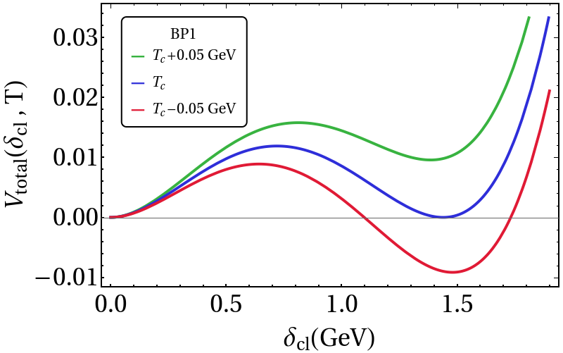
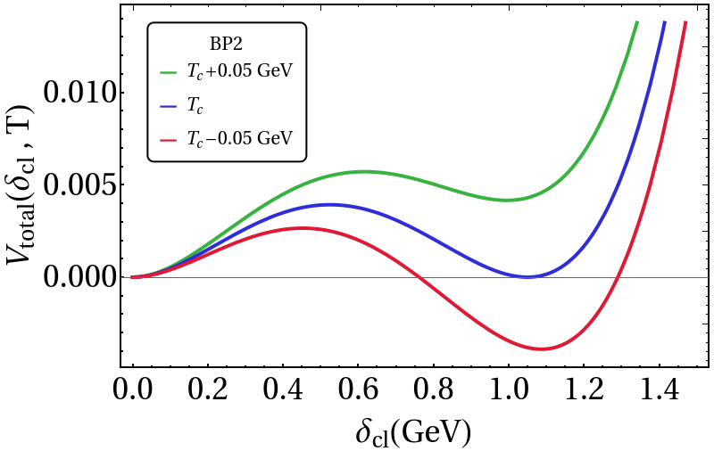
Figure 4: The extrema of the thermal potential around $T=T_{c}$ for BP1 and BP2. The color coding is shown in the legends.

Both BP1 and BP2 correspond to sub-GeV critical temperatures. One also inspects in Fig.4 that $\delta(T_{c})\gtrsim$ 1 GeV for both thereby signalling a SFOPT.

	$\lambda_{11}$	$\lambda_{12}$	$\lambda_{22}$	$\lambda_{23}$	$\mu_{22}$ (GeV)	$m_{h_{2}}$ (GeV)	$m_{\phi}$ (GeV)	$v_{\delta}$ (GeV)	$\mu_{21}$ (GeV)	$T_{c}$ (GeV)	$\frac{\delta(T_{c})}{T_{c}}$	$\Omega_{\text{D}M}h^{2}$
BP1	0.1	4.69202	0.0060999	0.00001	-0.208174	0.0647581	0.050095	66.8	0.756	0.975268	1.47608	0.114796
BP2	0.5	5.39401	0.0060999	0.00001	-0.144512	0.116026	0.0830917	45.3	0.586	0.717489	1.46328	0.114441

Table 1: Benchmark model parameters along with the predicted relic densities and the crtical temperatures.

	$T_{n}$ (GeV)	$\alpha$	$\beta/H$	$f_{\text{col}}$ (Hz)	$f_{\text{sw}}$ (Hz)	$f_{\text{tur}}$ (Hz)
BP1	0.821609	0.00931039	1119.22	4.16229 $\times 10^{-5}$	2.71898 $\times 10^{-4}$	3.86382 $\times 10^{-4}$
BP2	0.606572	0.009944	1149.43	3.15148 $\times 10^{-5}$	2.0544 $\times 10^{-4}$	2.91941 $\times 10^{-4}$

Table 2: The nucleation temperature and other GW parameters corresponding to BP1 and BP2.

A combined analysis of the relic density and SFOPT is in order. We first fix $\lambda_{13}=\lambda_{23}=10^{-5},~{}\lambda_{11}=0.1,~{}0.5,~{}1$ and vary the rest of the parameters as $|\sin\theta|<0.001,~{}|\lambda_{12}|<6,~{}|\lambda_{22}|<6,~{}|\mu_{21}|<1~{}\text{GeV},~{}1~{}\text{MeV}<m_{\phi}<1~{}\text{GeV},~{}1~{}\text{MeV}<m_{h_{2}}<2m_{\phi}$. It can be noted that the small values taken for sin$\theta$ and $\lambda_{13}$ render the $\phi-\phi-h_{1(2)}$ interactions appropriately small so as to conform with possible stringent direct detection bounds in the near future. The small sin$\theta$ also implies safety from the Higgs signal strength constraints and the direct search constraints involving $h_{2}$. The full thermal potential is analysed using the publicly available tool PhaseTracer Athron:2020sbe . We select the parameter points that lead to (a) $0.1118<\Omega h^{2}<0.1280$ Planck:2018vyg and (b) $\frac{\delta_{\text{min}}(T_{c})}{T_{c}}>1$. The results are shown as plots in the $m_{\phi}-\lambda_{12}$ plane in Fig.5.

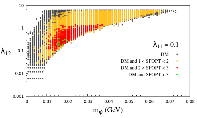
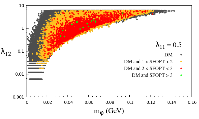
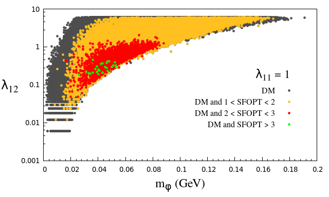
Figure 5: Parameter points in the $m_{\phi}-\lambda_{12}$ plane allowed by $\Omega h^{2}$ and SFOPT criteria for $\lambda_{11}$ = 0.1 (top left), 0.5 (top right) and 1 (bottom). The color coding is described in the legends.

Fig.5 shows a $\mathcal{O}$(10)-$\mathcal{O}$(100)(MeV) mass range for the DM thereby corroborating the results of Mohanty:2019drv . The correlation among $m_{\phi}$, $\lambda_{11}$ and $\lambda_{12}$ can be understood from $(\sigma v^{2})_{\phi\phi\phi\to\phi h_{2}}\sim\frac{\lambda^{2}_{11}(\mu_{21}+\lambda_{12}v_{\delta})^{2}}{m^{7}_{\phi}}$ in Eq.(10). The maximum allowed value of $m_{\phi}$ increases with increasing $\lambda_{11}$. And this is concurred by Fig.5 where one inspects that for the aforesaid variation of $\lambda_{12}$, changing $\lambda_{11}=0.1$ to $\lambda_{11}=1$ takes one from $m_{\phi}\lesssim$ 70 MeV to $m_{\phi}\lesssim$ 190 MeV. Demanding a SFOPT restricts the parameter space further.

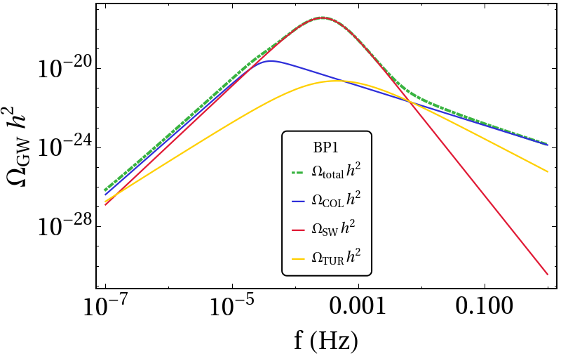
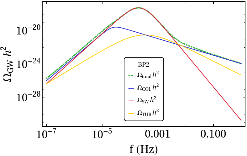
Figure 6: The nucleation temperature and other GW parameters corresponding to BP1 and BP2.

We now discuss the GW spectrum of such a scenario and a few pertinent quantities are therefore introduced. The parameter $\beta$ is defined as

$$\frac{\beta}{H} = \bigg{[}T\frac{d}{dT}\Big{(}\frac{S_{3}}{T}\Big{)}\bigg{]}_{T_{n}}.$$ (24)

Here, $T_{n}$ is the nucleation temperature and $S_{3}$ is the Euclidean action in three dimensions. Next, we define $\Delta V_{\text{tot}}(T)\equiv V_{\text{tot}}(0,T)-V_{\text{tot}}(\delta_{\text{min}}(T),T)$ which measures the difference in the depths of the potential at the two vacua at a temperature $T$. The energy budget of the phase transition during the bubble nucleation is then given by

$$\epsilon = \Delta V_{\text{tot}}(T_{n})-\bigg{[}T\frac{d\Delta V_{\text{tot}}(T)}{dT}\bigg{]}_{T_{n}}.$$ (25)

One subsequently defines $\alpha=\frac{\epsilon}{\rho_{n}}$, where $\rho_{n}=\frac{g_{*}\pi^{2}}{30}T_{n}^{4}$, is the energy density during nucleation. The sources of GWs associated with SFOPT are bubble collision Kosowsky ; Turner ; Huber_2008 ; Watkins ; Marc ; Caprini_2008 , sound waves Hindmarsh ; Leitao:2012tx ; Giblin:2013kea ; Giblin:2014qia ; Hindmarsh_2015 , and, magnetohydrodynamic turbulence Chiara ; Kahniashvili ; Kahniashvili:2008pe ; Kahniashvili:2009mf ; Caprini:2009yp . The GW amplitudes from these sources are functions of the frequency. These amplitudes attain their maximum values at certain “peak frequencies” that we denote as $f_{\text{col}},f_{\text{sw}}$ and $f_{\text{tur}}$. The expressions for these frequencies and the corresponding GW amplitudes is given in the Appendix V.

The $\alpha$ and $\beta$ parameters are crucial in deciding the strength of the GW signals stemming from a SFOPT. Table 2 displays $T_{n},\alpha,\beta$ for the chosen benchmarks. Bubble nucleation at the sub-GeV temperatures shown can be understood as an artefact of the sub-GeV DM masses involved. This is an important observation of our analysis. We also inspect in table 2 that $\alpha$ and $\beta/H$ at nucleation are respectively $\mathcal{O}(10^{-3})$ and $\mathcal{O}(10^{3})$ for the BPs. Such ball-park values entail that the magnitude of the total GW amplitude peaks at $\mathcal{O}(10^{-18})$, as is seen in Fig.6. And the corresponding frequencies are $\sim\mathcal{O}(10^{-4})$ Hz. This is expected since the total GW amplitude is dominated by the sound wave component that has $f_{\text{sw}}\sim\mathcal{O}(10^{-4})$ Hz. Overall, an $\Omega_{\text{GW}}h^{2}\sim\mathcal{O}(10^{-18})$ with peak at $f\sim\mathcal{O}(10^{-4})$ Hz is beyond the reach of the proposed GW detectors. However, u-DECIGO Kudoh:2005as is expected to detect GW signals of a similar magnitude, albeit at a different frequency range. In all, a future detector with higher sensitivity in the $\sim\mathcal{O}$(0.1) mHz regime can potentially detect GW signals of a sub-GeV DM species exhibiting number changing annihilations.

IV Conclusions

In this study, we look at possible GW signals originating from a SIMP. The SIMP species freezes-out via $3\to 2$ number changing processes that are in turn driven by another scalar $\delta$. The observed relic density is attained for sub-GeV DM masses. We have studied the shape of the thermal potential along $\delta$ and identified the region of the parameter space permitting a SFOPT. For a few representative benchmarks, we have then computed the GW amplitude as a function of frequency. Our analysis reveals that a futuristic detector with a sensitivity $\Omega_{\text{GW}}h^{2}\sim 10^{-18}$ in the mHz regime can detect GWs stemming from such a SIMP framework.

V Appendix

The peak frequencies corresponding to bubble collisions, sound waves and turbulence are expressed as

$$f_{\text{col}} = 1.65\times 10^{-5}\Big{(}\frac{0.62}{1.8-0.1v_{b}+v^{2}_{b}}\Big{)}$$ (26a)

$$\frac{\beta}{H}\Big{(}\frac{T_{n}}{100}\Big{)}\Big{(}\frac{g_{*}}{100}\Big{)}^{\frac{1}{6}},$$

$$f_{\text{sw}} = 1.9\times 10^{-5}\Big{(}\frac{1}{v_{b}}\Big{)}\frac{\beta}{H}\Big{(}\frac{T_{n}}{100}\Big{)}\Big{(}\frac{g_{*}}{100}\Big{)}^{\frac{1}{6}},$$ (26b)

$$f_{\text{tur}} = 2.7\times 10^{-5}\Big{(}\frac{1}{v_{b}}\Big{)}\frac{\beta}{H}\Big{(}\frac{T_{n}}{100}\Big{)}\Big{(}\frac{g_{*}}{100}\Big{)}^{\frac{1}{6}}.$$ (26c)

We express below the GW amplitudes from the three sources as a function of frequency $f$.

$$\Omega_{\text{coll}}(f) = 1.67\times 10^{-5}\Big{(}\frac{\beta}{H}\Big{)}^{-2}\Big{(}\frac{0.11v^{3}_{b}}{0.42+v^{2}_{b}}\Big{)}\Big{(}\frac{\kappa\alpha}{1+\alpha}\Big{)}^{2}$$ (27)

$$\Big{(}\frac{g_{*}}{100}\Big{)}^{-\frac{1}{3}}\Big{(}\frac{3.8(f/f_{\text{coll}})^{2.8}}{1+2.8(f/f_{\text{coll}})^{3.8}}\Big{)}$$

$$\Omega_{\text{sw}}(f) = 2.65\times 10^{-6}\Big{(}\frac{\beta}{H}\Big{)}^{-2}v_{b}\Big{(}\frac{\kappa_{v}\alpha}{1+\alpha}\Big{)}^{2}$$ (28)

$$\Big{(}\frac{g_{*}}{100}\Big{)}^{-\frac{1}{3}}\Big{(}\frac{f}{f_{\text{sw}}}\Big{)}^{3}\Big{(}\frac{7}{4+3(f/f_{\text{sw}})^{2}}\Big{)}^{2},$$

$$\Omega_{\text{tur}}(f) = 3.35\times 10^{-4}\Big{(}\frac{\beta}{H}\Big{)}^{-2}v_{b}\Big{(}\frac{\epsilon\kappa_{v}\alpha}{1+\alpha}\Big{)}^{1.5}$$ (29)

$$\Big{(}\frac{g_{*}}{100}\Big{)}^{-\frac{1}{3}}\Big{(}\frac{f}{f_{\text{tur}}}\Big{)}^{3}\frac{(1+f/f_{\text{tur}})^{-11/3}}{1+8\pi f/h_{s}}.$$

VI Acknowledgements

NC acknowledges support from DST, India, under grant number IFA18-PH214 (INSPIRE Faculty Award). HR is supported by the Science and Engineering Research Board, Government of India, under the agreement SERB/PHY/2016348 (Early Career Research Award). TS acknowledges the support from the Dr. D. S. Kothari Postdoctoral scheme No. PH/20-21/0163.

References

- (1) V. C. Rubin and W. K. Ford, Jr., Rotation of the Andromeda Nebula from a Spectroscopic Survey of Emission Regions, Astrophys. J. 159 (1970) 379–403.
- (2) G. Bertone, D. Hooper and J. Silk, Particle dark matter: Evidence, candidates and constraints, Phys. Rept. 405 (2005) 279–390, [hep-ph/0404175].
- (3) W. Hu and S. Dodelson, Cosmic Microwave Background Anisotropies, Ann. Rev. Astron. Astrophys. 40 (2002) 171–216, [astro-ph/0110414].
- (4) WMAP collaboration, G. Hinshaw et al., Nine-Year Wilkinson Microwave Anisotropy Probe (WMAP) Observations: Cosmological Parameter Results, Astrophys. J. Suppl. 208 (2013) 19, [1212.5226].
- (5) Planck collaboration, N. Aghanim et al., Planck 2018 results. VI. Cosmological parameters, Astron. Astrophys. 641 (2020) A6, [1807.06209].
- (6) G. R. Blumenthal, S. M. Faber, J. R. Primack and M. J. Rees, Formation of Galaxies and Large Scale Structure with Cold Dark Matter, Nature 311 (1984) 517–525.
- (7) E. W. Kolb and M. S. Turner, The Early Universe, vol. 69. 1990, 10.1201/9780429492860.
- (8) G. Jungman, M. Kamionkowski and K. Griest, Supersymmetric dark matter, Phys. Rept. 267 (1996) 195–373, [hep-ph/9506380].
- (9) J. L. Feng, Dark Matter Candidates from Particle Physics and Methods of Detection, Ann. Rev. Astron. Astrophys. 48 (2010) 495–545, [1003.0904].
- (10) G. Arcadi, M. Dutra, P. Ghosh, M. Lindner, Y. Mambrini, M. Pierre et al., The waning of the WIMP? A review of models, searches, and constraints, Eur. Phys. J. C 78 (2018) 203, [1703.07364].
- (11) L. Roszkowski, E. M. Sessolo and S. Trojanowski, WIMP dark matter candidates and searches—current status and future prospects, Rept. Prog. Phys. 81 (2018) 066201, [1707.06277].
- (12) XENON collaboration, E. Aprile et al., Dark Matter Search Results from a One Ton-Year Exposure of XENON1T, Phys. Rev. Lett. 121 (2018) 111302, [1805.12562].
- (13) LUX collaboration, D. S. Akerib et al., Limits on spin-dependent WIMP-nucleon cross section obtained from the complete LUX exposure, Phys. Rev. Lett. 118 (2017) 251302, [1705.03380].
- (14) D. Abercrombie et al., Dark Matter benchmark models for early LHC Run-2 Searches: Report of the ATLAS/CMS Dark Matter Forum, Phys. Dark Univ. 27 (2020) 100371, [1507.00966].
- (15) N. Bernal and X. Chu, SIMP Dark Matter, JCAP 1601 (2016) 006, [1510.08527].
- (16) S.-M. Choi and H. M. Lee, Resonant SIMP dark matter, Phys. Lett. B758 (2016) 47–53, [1601.03566].
- (17) S.-M. Choi, Y.-J. Kang and H. M. Lee, On thermal production of self-interacting dark matter, JHEP 12 (2016) 099, [1610.04748].
- (18) N. Bernal, X. Chu and J. Pradler, Simply split strongly interacting massive particles, Phys. Rev. D95 (2017) 115023, [1702.04906].
- (19) B. Chauhan, Sub-MeV Self Interacting Dark Matter, Phys. Rev. D97 (2018) 123017, [1711.02970].
- (20) S. Mohanty, A. Patra and T. Srivastava, MeV scale model of SIMP dark matter, neutrino mass and leptogenesis, JCAP 03 (2020) 027, [1908.00909].
- (21) S. Bhattacharya, P. Ghosh and S. Verma, SIMPler realisation of Scalar Dark Matter, JCAP 01 (2020) 040, [1904.07562].
- (22) H. M. Lee and M.-S. Seo, Communication with SIMP dark mesons via Z’ -portal, Phys. Lett. B 748 (2015) 316–322, [1504.00745].
- (23) N. Yamanaka, S. Fujibayashi, S. Gongyo and H. Iida, Dark Matter in the Nonabelian Hidden Gauge Theory, in 2nd Toyama International Workshop on Higgs as a Probe of New Physics, 4, 2015. 1504.08121.
- (24) Y. Hochberg, E. Kuflik and H. Murayama, SIMP Spectroscopy, JHEP 05 (2016) 090, [1512.07917].
- (25) Y. Hochberg, E. Kuflik, H. Murayama, T. Volansky and J. G. Wacker, Model for Thermal Relic Dark Matter of Strongly Interacting Massive Particles, Phys. Rev. Lett. 115 (2015) 021301, [1411.3727].
- (26) S.-M. Choi, Y. Hochberg, E. Kuflik, H. M. Lee, Y. Mambrini, H. Murayama et al., Vector SIMP dark matter, JHEP 10 (2017) 162, [1707.01434].
- (27) S.-M. Choi, H. M. Lee, P. Ko and A. Natale, Unitarizing SIMP scenario with dark vector resonances, PoS ICHEP2018 (2019) 036, [1811.02751].
- (28) J. Herms, A. Ibarra and T. Toma, A new mechanism of sterile neutrino dark matter production, JCAP 06 (2018) 036, [1802.02973].
- (29) E. Ma, N. Pollard, R. Srivastava and M. Zakeri, Gauge Model with Residual Symmetry, Phys. Lett. B 750 (2015) 135–138, [1507.03943].
- (30) E. Thrane and J. D. Romano, Sensitivity curves for searches for gravitational-wave backgrounds, Phys. Rev. D 88 (2013) 124032, [1310.5300].
- (31) B. Sathyaprakash et al., Scientific Objectives of Einstein Telescope, Class. Quant. Grav. 29 (2012) 124013, [1206.0331].
- (32) LISA collaboration, P. Amaro-Seoane et al., Laser Interferometer Space Antenna, 1702.00786.
- (33) J. Crowder and N. J. Cornish, Beyond LISA: Exploring future gravitational wave missions, Phys. Rev. D 72 (2005) 083005, [gr-qc/0506015].
- (34) N. Seto, S. Kawamura and T. Nakamura, Possibility of direct measurement of the acceleration of the universe using 0.1-Hz band laser interferometer gravitational wave antenna in space, Phys. Rev. Lett. 87 (2001) 221103, [astro-ph/0108011].
- (35) S. Sato et al., The status of DECIGO, J. Phys. Conf. Ser. 840 (2017) 012010.
- (36) L. Lentati et al., European Pulsar Timing Array Limits On An Isotropic Stochastic Gravitational-Wave Background, Mon. Not. Roy. Astron. Soc. 453 (2015) 2576–2598, [1504.03692].
- (37) G. Janssen et al., Gravitational wave astronomy with the SKA, PoS AASKA14 (2015) 037, [1501.00127].
- (38) M. Fairbairn, E. Hardy and A. Wickens, Hearing without seeing: gravitational waves from hot and cold hidden sectors, JHEP 07 (2019) 044, [1901.11038].
- (39) M. Breitbach, J. Kopp, E. Madge, T. Opferkuch and P. Schwaller, Dark, Cold, and Noisy: Constraining Secluded Hidden Sectors with Gravitational Waves, JCAP 07 (2019) 007, [1811.11175].
- (40) P. Schwaller, Gravitational Waves from a Dark Phase Transition, Phys. Rev. Lett. 115 (2015) 181101, [1504.07263].
- (41) J. Jaeckel, V. V. Khoze and M. Spannowsky, Hearing the signal of dark sectors with gravitational wave detectors, Phys. Rev. D 94 (2016) 103519, [1602.03901].
- (42) A. Addazi, Limiting First Order Phase Transitions in Dark Gauge Sectors from Gravitational Waves experiments, Mod. Phys. Lett. A 32 (2017) 1750049, [1607.08057].
- (43) I. Baldes, Gravitational waves from the asymmetric-dark-matter generating phase transition, JCAP 05 (2017) 028, [1702.02117].
- (44) K. Tsumura, M. Yamada and Y. Yamaguchi, Gravitational wave from dark sector with dark pion, JCAP 07 (2017) 044, [1704.00219].
- (45) I. Baldes and C. Garcia-Cely, Strong gravitational radiation from a simple dark matter model, JHEP 05 (2019) 190, [1809.01198].
- (46) D. Croon, V. Sanz and G. White, Model Discrimination in Gravitational Wave spectra from Dark Phase Transitions, JHEP 08 (2018) 203, [1806.02332].
- (47) M. Kamionkowski, A. Kosowsky and M. S. Turner, Gravitational radiation from first order phase transitions, Phys. Rev. D 49 (1994) 2837–2851, [astro-ph/9310044].
- (48) E. Witten, Cosmic Separation of Phases, Phys. Rev. D 30 (1984) 272–285.
- (49) C. J. Hogan, Gravitational radiation from cosmological phase transitions, Mon. Not. Roy. Astron. Soc. 218 (1986) 629–636.
- (50) C. Grojean and G. Servant, Gravitational Waves from Phase Transitions at the Electroweak Scale and Beyond, Phys. Rev. D 75 (2007) 043507, [hep-ph/0607107].
- (51) M. M. Pierre, Dark Matter phenomenology : from simplified WIMP models to refined alternative solutions. PhD thesis, U. Paris-Saclay, 2018. 1901.05822.
- (52) S. Bhattacharya, P. Poulose and P. Ghosh, Multipartite Interacting Scalar Dark Matter in the light of updated LUX data, JCAP 04 (2017) 043, [1607.08461].
- (53) S. Weinberg, Gauge and global symmetries at high temperature, Phys. Rev. D 9 (Jun, 1974) 3357–3378.
- (54) L. Dolan and R. Jackiw, Symmetry behavior at finite temperature, Phys. Rev. D 9 (Jun, 1974) 3320–3341.
- (55) D. A. Kirzhnits and A. D. Linde, Symmetry Behavior in Gauge Theories, Annals Phys. 101 (1976) 195–238.
- (56) M. E. Carrington, The Effective potential at finite temperature in the Standard Model, Phys. Rev. D 45 (1992) 2933–2944.
- (57) D. J. Gross, R. D. Pisarski and L. G. Yaffe, Qcd and instantons at finite temperature, Rev. Mod. Phys. 53 (Jan, 1981) 43–80.
- (58) P. Fendley, The Effective Potential and the Coupling Constant at High Temperature, Phys. Lett. B 196 (1987) 175–180.
- (59) J. Kapusta, Finite temperature Field Theory, Cambridge University Press (1989) .
- (60) P. B. Arnold and O. Espinosa, The Effective potential and first order phase transitions: Beyond leading-order, Phys. Rev. D 47 (1993) 3546, [hep-ph/9212235].
- (61) R. R. Parwani, Resummation in a hot scalar field theory, Phys. Rev. D 45 (1992) 4695, [hep-ph/9204216].
- (62) M. Quiros, Finite temperature field theory and phase transitions, in ICTP Summer School in High-Energy Physics and Cosmology, pp. 187–259, 1, 1999. hep-ph/9901312.
- (63) P. Athron, C. Balázs, A. Fowlie and Y. Zhang, PhaseTracer: tracing cosmological phases and calculating transition properties, Eur. Phys. J. C 80 (2020) 567, [2003.02859].
- (64) A. Kosowsky, M. S. Turner and R. Watkins, Gravitational radiation from colliding vacuum bubbles, Phys. Rev. D 45 (Jun, 1992) 4514–4535.
- (65) A. Kosowsky and M. S. Turner, Gravitational radiation from colliding vacuum bubbles: Envelope approximation to many-bubble collisions, Phys. Rev. D 47 (May, 1993) 4372–4391.
- (66) S. J. Huber and T. Konstandin, Gravitational wave production by collisions: more bubbles, Journal of Cosmology and Astroparticle Physics 2008 (Sep, 2008) 022.
- (67) A. Kosowsky, M. S. Turner and R. Watkins, Gravitational waves from first-order cosmological phase transitions, Phys. Rev. Lett. 69 (Oct, 1992) 2026–2029.
- (68) M. Kamionkowski, A. Kosowsky and M. S. Turner, Gravitational radiation from first-order phase transitions, Phys. Rev. D 49 (Mar, 1994) 2837–2851.
- (69) C. Caprini, R. Durrer and G. Servant, Gravitational wave generation from bubble collisions in first-order phase transitions: An analytic approach, Physical Review D 77 (Jun, 2008) .
- (70) M. Hindmarsh, S. J. Huber, K. Rummukainen and D. J. Weir, Gravitational waves from the sound of a first order phase transition, Phys. Rev. Lett. 112 (Jan, 2014) 041301.
- (71) L. Leitao, A. Megevand and A. D. Sanchez, Gravitational waves from the electroweak phase transition, JCAP 10 (2012) 024, [1205.3070].
- (72) J. T. Giblin, Jr. and J. B. Mertens, Vacuum Bubbles in the Presence of a Relativistic Fluid, JHEP 12 (2013) 042, [1310.2948].
- (73) J. T. Giblin and J. B. Mertens, Gravitional radiation from first-order phase transitions in the presence of a fluid, Phys. Rev. D 90 (2014) 023532, [1405.4005].
- (74) M. Hindmarsh, S. J. Huber, K. Rummukainen and D. J. Weir, Numerical simulations of acoustically generated gravitational waves at a first order phase transition, Physical Review D 92 (Dec, 2015) .
- (75) C. Caprini and R. Durrer, Gravitational waves from stochastic relativistic sources: Primordial turbulence and magnetic fields, Phys. Rev. D 74 (Sep, 2006) 063521.
- (76) T. Kahniashvili, A. Kosowsky, G. Gogoberidze and Y. Maravin, Detectability of gravitational waves from phase transitions, Phys. Rev. D 78 (Aug, 2008) 043003.
- (77) T. Kahniashvili, L. Campanelli, G. Gogoberidze, Y. Maravin and B. Ratra, Gravitational Radiation from Primordial Helical Inverse Cascade MHD Turbulence, Phys. Rev. D 78 (2008) 123006, [0809.1899].
- (78) T. Kahniashvili, L. Kisslinger and T. Stevens, Gravitational Radiation Generated by Magnetic Fields in Cosmological Phase Transitions, Phys. Rev. D 81 (2010) 023004, [0905.0643].
- (79) C. Caprini, R. Durrer and G. Servant, The stochastic gravitational wave background from turbulence and magnetic fields generated by a first-order phase transition, JCAP 12 (2009) 024, [0909.0622].
- (80) H. Kudoh, A. Taruya, T. Hiramatsu and Y. Himemoto, Detecting a gravitational-wave background with next-generation space interferometers, Phys. Rev. D 73 (2006) 064006, [gr-qc/0511145].