Tests of general relativity in the nonlinear regime: a parametrized
plunge-merger-ringdown gravitational waveform model

Abstract

The plunge-merger stage of the binary-black-hole coalescence, when the bodies’ velocities reach a large fraction of the speed of light and the gravitational-wave luminosity peaks, provides a unique opportunity to probe gravity in the dynamical and nonlinear regime. How much do the predictions of general relativity differ from the ones in other theories of gravity for this stage of the binary evolution? To address this question, we develop a parametrized waveform model, within the effective-one-body formalism, that allows for deviations from general relativity in the plunge-merger-ringdown stage. As first step, we focus on nonprecessing-spin, quasicircular black hole binaries. In comparison to previous works, for each gravitational wave mode, our model can modify, with respect to general-relativistic predictions, the instant at which the amplitude peaks, the instantaneous frequency at this time instant, and the value of the peak amplitude. We use this waveform model to explore several questions considering both synthetic-data injections and two gravitational wave signals. In particular, we find that deviations from the peak gravitational wave amplitude and instantaneous frequency can be constrained to about 20% with GW150914. Alarmingly, we find that GW200129_065458 shows a strong violation of general relativity. We interpret this result as a false violation, either due to waveform systematics (mismodeling of spin precession) or due to data-quality issues depending on one’s interpretation of this event. This illustrates the use of parametrized waveform models as tools to investigate systematic errors in plain general relativity. The results with GW200129_065458 also vividly demonstrate the importance of waveform systematics and of glitch mitigation procedures when interpreting tests of general relativity with current gravitational wave observations.

I Introduction

Remarkably, so far, the theory of general relativity (GR), introduced by Albert Einstein in 1915, has passed all available experimental and observational tests Will (2014): on cosmological Clifton et al. (2012) and short scales Kapner et al. (2007); Lee et al. (2020), in the low-velocity, weak-field Abuter et al. (2020) and strong-field settings Kramer et al. (2021); Akiyama et al. (2019, 2022), and in the dynamical, high-velocity and strong-field regime Abbott et al. (2016a, 2019a, 2019b, 2021a, 2021b). The latter has been probed, since 2015, through the gravitational wave (GW) observation of the coalescence of binary black holes (BBHs) Abbott et al. (2016b, c, 2019c, 2021c, 2021d, 2021e), neutron-star–black-hole (BH) binaries Abbott et al. (2021f), and binary neutron stars Abbott et al. (2017, 2020) by the LIGO and Virgo detectors Aasi et al. (2015); Acernese et al. (2015).

Generally, tests of GR with GW observations have been developed following two strategies: theory independent and theory specific. The former assumes that the underlying GW signal is well-described by GR, and non-GR degrees of freedom (or parameters) are included to characterize any potential deviation. These tests use GW observations to check consistency with their nominal predictions in GR, and then constrain the non-GR parameters at a certain statistical level of confidence. Eventually, the non-GR parameters can be translated to the ones in specific modified theories of gravity, albeit there could be subtleties in doing it due to the choice of the priors and the actual parameters on which the measurements are done. By contrast, analyses that compare directly the data with proposed modified theories of gravity belong to the theory-specific framework of tests of GR.

Here, we focus on theory-independent tests of GR for BBHs. Historically, those tests have been proposed introducing deviations in (or parametrizations of) the gravitational waveform, whether for the inspiral, the merger or the ringdown stages, in time or frequency domain. Those parametrizations are clearly not unique; neither they guarantee to fully represent the infinite space of modified gravity-theory waveforms. Furthermore, non-GR parameters may be degenerate with each other, limiting the study to a subset of them Abbott et al. (2016a) or demanding the use of principal-component-analysis methods Saleem et al. (2022a).

Many parametrized waveforms have been suggested in the literature, originally focusing on the inspiral phase Blanchet and Sathyaprakash (1995); Arun et al. (2006a, b), when the BBH system slowly but steadily looses energy through GW emission, and the bodies come closer and closer to each other until they merge. When the first frequency-domain models for the inspiral-merger-ringdown (IMR) waveforms in GR became available Pan et al. (2008); Ajith et al. (2008), a parametrized frequency-domain IMR waveform model was proposed in Ref. Yunes and Pretorius (2009), variations of which were soon after employed in Ref. Sampson et al. (2014) for data-analysis explorations. Those initial works, together with other developments Gossan et al. (2012); Meidam et al. (2014), are at the foundation of the Test Infrastructure for GEneral Relativity (TIGER) Li et al. (2012); Agathos et al. (2014); Meidam et al. (2018), Flexible Theory Independent (FTI) Mehta et al. (2023), pSEOBNR Brito et al. (2018); Ghosh et al. (2021), and pyRing Carullo et al. (2018, 2019a); Isi et al. (2019a) pipelines, which today are routinely used by the LIGO-Virgo-KAGRA (LVK) Collaboration Abbott et al. (2016a, 2019a, 2019b, 2021a, 2021b) to perform parametrized tests of GR, probing the generation of GWs and the remnant properties, in the linear and nonlinear strong-field gravity regime. Other theory-independent tests were also performed, e.g., in Refs. Carullo et al. (2019b); Isi et al. (2019b); Tsang et al. (2020); Bhagwat and Pacilio (2021); Okounkova et al. (2022); Wang et al. (2022); Saleem et al. (2022b); Haegel et al. (2023).

In this manuscript, we develop a parametrized time-domain IMR waveform model within the effective-one-body (EOB) formalism Buonanno and Damour (1999, 2000); Damour et al. (2000); Damour (2001); Buonanno et al. (2006); Barausse and Buonanno (2010); Damour et al. (2009); Pan et al. (2011a). The EOB approach builds semianalytical IMR waveforms by combining analytical predictions for the inspiral [notably from post-Newtonian (PN), post-Minkowskian (PM), and gravitational self-force (GSF) approximations] and ringdown phases (from BH perturbation theory) with physically-motivated Ansätze for the plunge-merger stage. The EOB waveforms are then made highly accurate via a calibration to numerical relativity (NR) waveforms of BBHs. The EOB formalism relies on three key ingredients: the EOB conservative dynamics (i.e., a two-body Hamiltonian), the EOB radiation-reaction forces (i.e., the energy and angular momentum fluxes) and the EOB GW modes. Since the EOB waveforms are computed on the EOB dynamics by solving Hamilton’s equations, in principle deviations from GR can be introduced in all the three building blocks, consistently. Here, for simplicity, following previous work Brito et al. (2018); Ghosh et al. (2021) which focused on the ringdown stage, we introduce non-GR parameters in the plunge-merger-ringdown GW modes. We leave to future work the extension of the parametrization to the conservative and dissipative dynamics, notably by including in the EOB dynamics fractional deviations to the PN (as well as PM and GSF) terms, to NR-informed terms or specific new terms motivated by phenomena observed in modified gravity theories. We note that non-GR deviations in the EOB energy flux were implemented in Refs. Ghosh et al. (2016, 2018), and the corresponding EOB waveforms were used in IMR consistency and other tests of gravity in Refs. Ghosh et al. (2016, 2018); Johnson-McDaniel et al. (2022).

Although the parametrized IMR model can in principle be constructed for precessing spinning BBHs, as first step, we consider nonprecessing BHs. There are two main EOB families, SEOBNR (e.g., see Refs. Bohé et al. (2017); Cotesta et al. (2018); Ossokine et al. (2020)) and TEOBResumS (e.g., see Refs. Nagar et al. (2018, 2020); Gamba et al. (2022)). We consider here the former, and in particular we focus on the SEOBNRHM model developed in Refs. Bohé et al. (2017); Cotesta et al. (2018), which contains GW modes beyond the dominant quadrupole. We denote the parametrized version pSEOBNRHM. In Fig 1, we contrast a GR SEOBNRHM waveform with parameters similar to the first GW observation, GW150914, with a pSEOBNRHM waveform where the fractional deviations from GR are of the order of a few tens of percent. We can see that differences from GR occur just before, during, and after the merger stage, which is when the gravitational strain peaks.

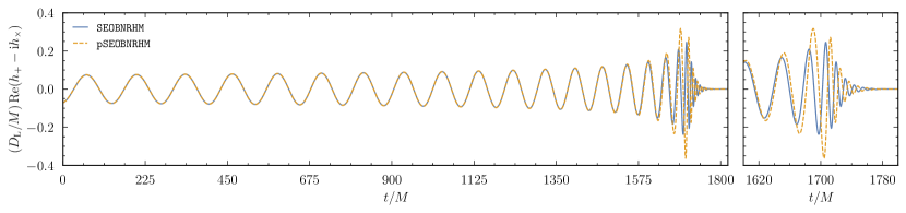
Figure 1: Illustrative BBH waveform obtained with the pSEOBNRHM model introduced here (dashed line) and the corresponding baseline model SEOBNRHM Boyle et al. (2008); Cotesta et al. (2018); Mihaylov et al. (2021) (solid line) for a face-on, nonspinning and quasicircular binary with GW150914-like mass-ratio $q=m_{2}/m_{1}\approx 0.867$, and detector-frame total mass $M=m_{1}+m_{2}=71.9~{}{\rm M}_{\odot}$. The pSEOBNRHM waveform is generated with non-GR parameters values $\delta\Delta t=-0.2$, $\delta\omega=-0.4$, and $\delta A=0.5$. These parameters change respectively, in comparison to GR, the instant at which the GW amplitude peaks, the orbital frequency at this time instant, and the value of the peak amplitude. Both waveforms are phase aligned and time shifted around $20$ Hz using the prescription of Refs. Boyle et al. (2008); Buonanno et al. (2009); Pan et al. (2011a, b). The details of how the waveform model is developed are in given Sec. II, and additional details about its morphology are presented in Sec. III.

The paper is organized as follows. In Sec. II, we describe how we build the pSEOBNRHM model starting from the baseline model SEOBNRHM, and introduce the non-GR parameters that describe potential deviations from GR during the plunge-merger-ringdown stage. In Sec. III, we study in detail the morphology of the parametrized waveform, and understand which parts of the waveform change when the non-GR parameters are varied one at the time. After discussing the basics of Bayesian analysis in Sec. IV, we perform a synthetic-signal injection study in Sec. V, and then apply our parametrized IMR model to real data in Secs. VI and VII, analyzing two events, GW150914 and GW200129. Finally, we summarize our conclusions and future work in Sec. VIII.

Unless stated otherwise, we work in geometrical units in which $G=1=c$.

II The parametrized plunge-merger-ringdown waveform model

In this section we first review the GR waveform model developed within the EOB formalism. In Sec. II.2, we explain how we deform this baseline model by introducing deformations away from GR in the plunge-merger-ringdown phase.

II.1 A brief review of the effective-one-body gravitational waveform model

The GW signal produced by a spinning, nonprecessing, and quasicircular BBH with component masses $m_{1}$ and $m_{2}$, and total mass $M=m_{1}+m_{2}$, is described in GR by a set of eleven parameters, $\bm{\vartheta}_{\rm GR}$, given by

$$\bm{\vartheta}_{\rm GR} =\left\{m_{1},m_{2},\chi_{1},\chi_{2},\iota,\psi,\alpha,\delta,D_{\rm L},t_{c},\phi_{c}\right\}\,,$$ (1)

where $\chi_{i}$ ($i=1,2)$ are the constant-in-time projections of each BH’s spin vectors $\bm{S}_{i}$ in the direction of the unit vector perpendicular to the orbital plane $\hat{\bm{L}}$, i.e., $\chi_{i}=\bm{S}_{i}\cdot\hat{\bm{L}}/m_{i}^{2}$, where $|\chi_{i}|\leqslant 1$, $(\iota,\psi)$ describe the binary’s orientation through the inclination and polarization angles, $(\alpha,\delta)$ describe the sky location of the source in the detector frame, $D_{\rm L}$ is the luminosity distance, and $t_{c}$ and $\phi_{c}$ are the reference time and phase, respectively. It is convenient to define the chirp mass ${\cal M}=M\nu^{3/5}$, where $\nu=m_{1}m_{2}/M^{2}$ is the symmetric mass ratio, the asymmetric mass ratio $q=m_{2}/m_{1}$, and the effective spin $\chi_{\rm eff}=(\chi_{1}m_{1}+\chi_{2}m_{2})/M$. We adopt the convention that $m_{1}\geqslant m_{2}$ and thus $q\leqslant 1$.

The GW polarizations can be written in the observer’s frame as

$$h_{+}(\iota,\varphi_{0};t)-{\rm i}h_{\times}(\iota,\varphi_{0};t)=\sum_{\ell=2}^{\infty}\sum_{m=-\ell}^{\ell}{}_{-2}Y_{\ell m}(\iota,\varphi_{0})h_{\ell m}(t),$$

where $\varphi_{0}$ is the azimuthal direction of the observer, where, without loss of generality, we set $\varphi_{0}=\phi_{c}$, and ${}_{-2}Y_{\ell m}$ are the $-2$ spin-weighted spherical harmonics Newman and Penrose (1966), $\ell$ is the angular number and $|m|\leqslant\ell$ is the azimuthal number of each GW mode, $h_{\ell m}$.

We follow Refs. Ghosh et al. (2021); Silva et al. (2023) and use as our baseline model (i.e., the waveform model upon which the non-GR deviation parameters are added) the time-domain IMR waveform developed in Refs. Bohé et al. (2017); Cotesta et al. (2018); Mihaylov et al. (2021) within the EOB formalism Buonanno and Damour (1999, 2000); Damour et al. (2000); Damour (2001); Buonanno et al. (2006); Barausse and Buonanno (2010); Damour et al. (2009); Pan et al. (2011a), SEOBNRv4HM_PA. The model uses the postadiabatic (PA) approximation, which was originally introduced in Refs. Damour et al. (2013); Nagar and Rettegno (2019); Rettegno et al. (2020) (and also subsequently used in the TEOBResumS waveform models) to speed up the generation of the time-domain waveforms for spinning, nonprecessing and quasicircular compact binaries. It includes the $(\ell,|m|)=(2,2)$, $(2,1)$, $(3,3)$, $(4,4)$, and $(5,5)$ GW modes. For nonprecessing BBHs (i.e., with component spins aligned or antialigned with the orbital angular momentum), we have that $h_{\ell m}=(-1)^{\ell}\,h_{\ell-m}^{\ast}$. Hence, we can consider $m>0$ without loss of generality. Hereafter, we refer to SEOBNRv4HM_PA as SEOBNRHM for brevity.

As explained in Refs. Bohé et al. (2017); Cotesta et al. (2018), the SEOBNRHM waveform is constructed by attaching the merger-ringdown waveform, $h_{\ell m}^{\rm merger-RD}(t)$, to the inspiral-plunge waveform, $h_{\ell m}^{\rm insp-plunge}(t)$, at a matching time $t=t^{\ell m}_{\rm match}$,

$$h_{\ell m}(t) =h_{\ell m}^{\rm insp-plunge}(t)\,\Theta\left(t_{\rm match}^{\ell m}-t\right)$$

$$\quad+h_{\ell m}^{\rm merger-RD}(t)\,\Theta\left(t-t_{\rm match}^{\ell m}\right)\,,$$ (3)

where $\Theta(t)$ is the Heaviside step function and the value of $t_{\rm match}^{\ell m}$ is defined as

$$t_{\rm match}^{\ell m}=\begin{cases}t^{22}_{\rm peak}\,,&(\ell,m)=(2,2),\,(3,3),\,(2,1),\\ &\qquad\quad\,\,\,\,\,(4,4)\\ t^{22}_{\rm peak}-10M\,,&(\ell,m)=(5,5)\,,\end{cases}$$ (4)

where $t^{22}_{\rm peak}$ is the time at which the amplitude of the $(2,2)$ mode [i.e., $h_{22}(t)$ in Eq. (LABEL:eq:hpc)] has its maximum value. We impose that the amplitude and phase of $h_{\ell m}(t)$ at $t=t^{\ell m}_{\rm match}$ are $C^{1}$ (i.e., they are continuously and differentiable at this time instant). The time $t^{22}_{\rm peak}$ is defined as

$$t^{22}_{\rm peak}=t^{\Omega}_{\rm peak}+\Delta t^{22}_{\rm peak}\,,$$ (5)

where $t^{\Omega}_{\rm peak}$ is the time in which the EOB orbital frequency peaks Taracchini et al. (2012). Calculations performed in the test-particle limit using BH perturbation theory found that the amplitude and the orbital frequency peak at different times, especially when the central BH has large spins Damour and Nagar (2007); Barausse et al. (2012); Taracchini et al. (2014a); Price and Khanna (2016). This motivates the introduction of the time-lag parameter $\Delta t^{22}_{\rm peak}$ in Eq. (5), which can be fitted against NR waveforms as function of the symmetric mass ratio $\nu$ and the BH’s spins $\chi_{1,2}$ (see Sec. II B in Ref. Bohé et al. (2017) for details). We impose the condition $\Delta t^{22}_{\rm peak}\leqslant 0$ to ensure that the attachment of the merger-ringdown waveform happens before the peak of the orbital frequency, and thus before the end of the binary’s dynamics. For later convenience, we define

$$\Delta t^{\rm GR}_{\ell m}=-\Delta t^{22}_{\rm peak}\,.$$ (6)

Because we are interested in adding non-GR terms to $h_{\ell m}^{\rm merger-RD}(t)$, we now briefly review how the merger-ringdown waveform is constructed. Further details can be found in Sec. IV E of Ref. Cotesta et al. (2018). The merger-ringdown mode is written as

$$h_{{\ell m}}^{\rm merger-RD}=\nu\,\tilde{A}_{{\ell m}}(t)\,e^{{\rm i}\tilde{\phi}_{\ell m}(t)}\,e^{{\rm i}\sigma_{{\ell m}0}(t-t^{{\ell m}}_{\rm match})}\,,$$ (7)

where $\sigma_{{\ell m}0}$ are the complex-valued frequencies of the least damped quasinormal mode (QNM) of the remnant BH Vishveshwara (1970); Press (1971); Detweiler (1980). We define $\sigma_{{\ell m}0}^{\rm R}={\rm Im}(\sigma_{{\ell m}0})<0$ and $\sigma_{{\ell m}0}^{\rm I}=-{\rm Re}(\sigma_{{\ell m}0})<0$. The functions $\tilde{A}_{{\ell m}}$ and $\tilde{\phi}_{\ell m}$ are given by Bohé et al. (2017)

$$\tilde{A}_{{\ell m}} =c_{1,c}^{{\ell m}}\,\tanh\left[c_{1,f}^{{\ell m}}\,(t-t^{\ell m}_{\rm match})+c_{2,f}^{{\ell m}}\right]+c_{2,c}^{{\ell m}}\,,$$ (8a)

$$\tilde{\phi}_{{\ell m}} =\phi^{{\ell m}}_{\rm match}-d_{1,c}^{{\ell m}}\,\log\left[\frac{1+d_{2,f}^{{\ell m}}\,e^{-d_{1,f}^{{\ell m}}(t-t^{\ell m}_{\rm match})}}{1+d_{2,f}^{{\ell m}}}\right]\,,$$

where $\phi^{{\ell m}}_{\rm match}$ is the phase of the inspiral-plunge mode $h_{{\ell m}}^{\rm insp-plunge}$ at $t=t^{{\ell m}}_{\rm match}$. We see that Eqs. (8) depend on the set of parameters $c^{{\ell m}}_{i}$ and $d^{{\ell m}}_{i}$ ($i=1,2$), which are either constrained by imposing that $\tilde{A}_{{\ell m}}$, $\tilde{\phi}_{{\ell m}}$ are $C^{1}$ at $t=t^{\ell m}_{\rm match}$ (we append the subscript “$c$”) or free parameters to be determined by fitting against NR waveforms (we append the subscript “$f$”).

We now impose that $h_{{\ell m}}$ is $C^{1}$ at $t=t^{\ell m}_{\rm match}$. This yields two equations that relate the constrained coefficients $c_{1,c}^{{\ell m}}$ and $c_{2,c}^{{\ell m}}$ to the free coefficients $c_{1,f}^{{\ell m}}$, $c_{2,f}^{{\ell m}}$, to $\sigma_{{\ell m}0}^{\rm R}$ and to the mode amplitude of $h_{{\ell m}}^{\rm insp-plunge}$ and its first time derivative at the matching time, namely $|h_{{\ell m}}^{\rm insp-plunge}(t^{\ell m}_{\rm match})|$ and $\partial_{t}|h_{{\ell m}}^{\rm insp-plunge}(t^{\ell m}_{\rm match})|$. The equations are:

$$c_{1,c}^{{\ell m}} =\frac{1}{\nu\,c_{1,f}^{{\ell m}}}\left[\partial_{t}|h_{{\ell m}}^{\rm insp-plunge}(t^{\ell m}_{\rm match})|\right.$$

$$\left.\quad-\sigma_{{\ell m}0}^{\rm R}\,|h_{{\ell m}}^{\rm insp-plunge}(t^{\ell m}_{\rm match})|\right]\,\cosh^{2}c_{2,f}^{{\ell m}}\,,$$ (9a)

$$c_{2,c}^{{\ell m}} =-\frac{1}{\nu}\,|h_{{\ell m}}^{\rm insp-plunge}(t^{\ell m}_{\rm match})|$$

$$\quad+\frac{1}{\nu\,c_{1,f}^{{\ell m}}}\left[\partial_{t}|h_{{\ell m}}^{\rm insp-plunge}(t^{\ell m}_{\rm match})|\right.$$

$$\left.\quad-\sigma_{{\ell m}0}^{\rm R}\,|h_{{\ell m}}^{\rm insp-plunge}(t^{\ell m}_{\rm match})|\right]\cosh c_{2,f}^{{\ell m}}\,\sinh c_{2,f}^{{\ell m}}\,.$$

We also obtain one equation that relates the constrained parameter $d_{1,c}^{{\ell m}}$ to the free coefficients $d_{1,f}^{{\ell m}}$, $d_{2,f}^{{\ell m}}$, to $\sigma_{{\ell m}0}^{\rm I}$ and to the angular frequency of $h_{{\ell m}}^{\rm insp-plunge}$ at the matching time. The latter is defined as $\omega_{{\ell m}}={\rm d}\phi^{\rm insp-plunge}_{{\ell m}}/{\rm d}t$, where $\phi^{\rm insp-plunge}_{{\ell m}}={\rm arg}(h^{\rm insp-plunge}_{{\ell m}})$ is the phase of the inspiral-plunge GW mode. The equation is,

$$d_{1,c}^{{\ell m}}=\left[\omega_{{\ell m}}^{\rm insp-plunge}(t^{\ell m}_{\rm match})-\sigma_{{\ell m}0}^{\rm I}\right]\,\frac{1+d_{2,f}^{{\ell m}}}{d_{1,f}^{{\ell m}}\ d_{2,f}^{{\ell m}}}\,.$$ (10)

The values of

$$|h_{{\ell m}}^{\rm insp-plunge}|,\quad\partial_{t}|h_{{\ell m}}^{\rm insp-plunge}|,\quad{\rm and}\quad\omega_{{\ell m}}^{\rm insp-plunge}\,,$$

at $t=t^{\ell m}_{\rm match}$ are fixed by the so-called nonquasicircular (NQC) terms, $N_{\ell m}(t)$. The NQC terms describe nonquasicircular corrections to the modes during the late inspiral and plunge. The NQCs are a parametrized time series that is multiplied with the factorized PN GR modes, $h_{{\ell m}}^{\rm F}$, such that the resultant time series is calibrated against NR simulations. They are crucial in guaranteeing a very good agreement of the SEOBNRHM amplitude and phase (relative to NR) during the late inspiral and plunge.

The GW modes in the inspiral-plunge part of the EOB waveform are given as

$$h^{\rm insp-plunge}_{{\ell m}}(t)=h_{{\ell m}}^{\rm F}(t)\,N_{{\ell m}}(t)\,,$$ (11)

where we refer the reader to Sec. IV C in Ref. Cotesta et al. (2018) for details on how $h_{{\ell m}}^{\rm F}$ and $N_{{\ell m}}$ are constructed. For our purposes, it is sufficient to say that $|h_{{\ell m}}^{\rm insp-plunge}|(t^{\ell m}_{\rm match})$, $\partial_{t}|h_{{\ell m}}^{\rm insp-plunge}(t^{\ell m}_{\rm match})|$, and $\omega_{{\ell m}}^{\rm insp-plunge}(t^{\ell m}_{\rm match})$ are the same as the NR values of

$$|h_{{\ell m}}^{\rm NR}|,\quad\partial_{t}|h_{{\ell m}}^{\rm NR}|,\quad{\rm and}\quad\omega_{{\ell m}}^{\rm NR}\,,$$

at $t=t^{\ell m}_{\rm match}$. The values of these three quantities are obtained for each BBH, from the Simulating eXtreme Spacetimes (SXS) catalog of NR waveforms Boyle et al. (2019), after which a fitting formula that depends on the symmetric mass ratio $\nu$ and spins $\chi_{1}$ and $\chi_{2}$ is obtained to interpolate over the parameter space covered by the catalog. Their explicit forms can be found in Ref. Cotesta et al. (2018), Appendix B. At this point, we are left with the free parameters $c_{i,f}^{{\ell m}}$ and $d_{i,f}^{{\ell m}}$ ($i=1,2$) to fix. This is accomplished through fits against NR and Teukolsky equation-based waveforms Barausse et al. (2012); Taracchini et al. (2014a), written also as functions of $\nu$, $\chi_{1}$ and $\chi_{2}$. The explicit form of these fits can be found in Ref. Cotesta et al. (2018), Appendix C.

II.2 Construction of the parametrized model

With this framework established, our strategy to develop a parametrized SEOBNRHM model (hereafter pSEOBNRHM) is the following. We will introduce fractional deviations to the NR-informed formulas for the mode amplitudes and angular frequencies at $t=t^{\ell m}_{\rm match}$, i.e.,

$$|h_{{\ell m}}^{\rm NR}| \to|h_{{\ell m}}^{\rm NR}|\,(1+\delta A_{{\ell m}})\,,$$ (12a)

$$\omega_{{\ell m}}^{\rm NR} \to\omega_{{\ell m}}^{\rm NR}\,(1+\delta\omega_{{\ell m}})\,,$$ (12b)

and we will also allow for changes to $t^{\ell m}_{\rm match}$ by modifying the time-lag parameter $\Delta t^{\rm GR}_{\ell m}$ [defined in Eq. (6)] as,

$$\Delta t^{\rm GR}_{\ell m}\to\Delta t^{\rm GR}_{\ell m}\,\left(1+\delta\Delta t_{\ell m}\right)\,,$$ (13)

where we constrain $\delta\Delta t_{{\ell m}}>-1$ to ensure that $t^{\ell m}_{\rm match}$ remains less than $t_{\rm peak}^{\Omega}$, and thus before the end of the dynamics, as originally required Boyle et al. (2008); Cotesta et al. (2018). Equations (12) and (13) modify the constrained parameters $c_{i,c}^{\ell m}$ and $d_{i,c}^{\ell m}$ through Eqs. (9)-(10), and consequently $\tilde{A}_{\ell m}$ and $\tilde{\phi}_{\ell m}$ that appear in the merger-ringdown waveform (7) and are given by Eqs. (8). It is important to emphasize that Eqs. (12) and (13) also modify the NQC coefficients which enter the inspiral-plunge waveform in Eq. (11). This is because both $|h_{\ell m}^{\rm NR}|$ and $\omega_{\ell m}^{\rm NR}$ are used to fix some parameters in the explicit form of $N_{\ell m}$. We refer the reader to Refs. Taracchini et al. (2014b); Bohé et al. (2017) and in particular to Ref. Cotesta et al. (2018), Sec. III C, for details. Hence, although we will refer to $\delta A_{\ell m}$, $\delta\omega_{\ell m}$, and $\delta\Delta t_{\ell m}$ as “merger parameters” they, strictly speaking, also modify the plunge.

We also introduce non-GR deformations to the QNMs, following the same strategy applied in Refs. Gossan et al. (2012); Meidam et al. (2014); Brito et al. (2018); Isi et al. (2019a); Ghosh et al. (2021); Isi and Farr (2021). It consists in modifying the QNM oscillation frequency and damping time, defined respectively for the zero overtone $n=0$, as,

$$f_{{\ell m}0} =\frac{1}{2\pi}{\rm Re}(\sigma_{{\ell m}0})=-\frac{1}{2\pi}\sigma^{\rm I}_{{\ell m}0}\,,$$ (14a)

$$\tau_{{\ell m}0} =-\frac{1}{{\rm Im}(\sigma_{{\ell m}0})}=-\frac{1}{\sigma^{\rm R}_{{\ell m}0}}\,,$$ (14b)

according to the substitutions

$$f_{{\ell m}0} \to f_{{\ell m}0}\,(1+\delta f_{{\ell m}0})\,,$$ (15a)

$$\tau_{{\ell m}0} \to\tau_{{\ell m}0}\,(1+\delta\tau_{{\ell m}0})\,,$$ (15b)

and we impose that $\delta\tau_{\ell m0}>-1$ to ensure that the remnant BH is stable (i.e., it rings downs, instead of “ringing-up” exponentially). Note that in Refs. Brito et al. (2018); Ghosh et al. (2021), such deformations also concerned with the higher overtones, since the EOB model used for the merger-ringdown included higher overtones.

Put it all together, we have the following set of plunge-merger-ringdown parameters:

$$\bm{\vartheta}_{\rm nGR} =\bm{\vartheta}_{\rm nGR}^{\rm merger}\,\cup\,\bm{\vartheta}_{\rm nGR}^{\rm RD}$$ (16)

$$=\left\{\delta A_{{\ell m}},\delta\omega_{{\ell m}},\delta\Delta t_{{\ell m}}\right\}\,\cup\,\left\{\delta f_{{\ell m}0},\delta\tau_{{\ell m}0}\right\}\,,$$

intended to capture possible signatures of beyond-GR physics in the most dynamical and nonlinear stage of a BBH coalescence. We will casually refer to them as “non-GR” or as “deformation” (away from GR) parameters. In Table 1, we summarize the $\bm{\vartheta}_{\rm nGR}$ parameters, their meaning, and the constraints, if any, on their values. The GR limit is recovered when all parameters in $\bm{\vartheta}_{\rm nGR}$ are set to zero.

	Parameter	Deformation	Bound
merger	$\delta A_{\ell m}$	amplitude
	$\delta\omega_{\ell m}$	instantaneous frequency
	$\delta\Delta t_{\ell m}$	time lag	$>-1$
ringdown	$\delta f_{\ell m0}$	oscillation frequency
	$\delta\tau_{\ell m0}$	damping time	$>-1$

Table 1: Summary of the non-GR parameters in the pSEOBNRHM model. The ringdown deformation parameters $\delta f_{\ell m0}$ and $\delta\tau_{\ell m0}$ were introduced to the SEOBNRHM model in Ref. Ghosh et al. (2021), while the merger deformation parameters $\delta A_{\ell m}$, $\delta\omega_{\ell m}$, and $\delta\Delta t_{\ell m}$ are introduced here for the first time. As explained in Sec. II.2, although we call these merger parameters, they do also affect the late inspiral-plunge part of the waveform. We quote under the column labeled “bound” the constraints on the parameter’s values required by our waveform model.

The pSEOBNRHM model allows us to change the non-GR plunge-merger parameters $\bm{\vartheta}_{\rm nGR}^{\rm merger}$ for each ($\ell$, $m$) mode individually. Here, for a first study, we will assume that their values are the same across different modes, that is to say,

$$\delta A_{{\ell m}}=\delta A,\,\delta\omega_{{\ell m}}=\delta\omega,\,\,\textrm{and}\,\,\delta\Delta t_{{\ell m}}=\delta\Delta t\,,$$ (17)

for all the $\ell$ and $m$ modes in the waveform model. This choice is motivated by the fact that in GW150914 there are no significant changes in the posterior distributions of the binary parameters when using all the modes and only the $\ell=m=2$ mode. As for the non-GR ringdown parameters $\bm{\vartheta}_{\rm nGR}^{\rm RD}$, we will assume that they are nonzero only for the least-damped ($n=0$) $(2,2)$ mode. Under these assumptions, we have a 16-dimensional parameter space to work with,

$$\bm{\vartheta}=\bm{\vartheta}_{\rm GR}\,\cup\,\bm{\vartheta}_{\rm nGR}\,,$$ (18)

where the GR parameters $\bm{\vartheta}_{\rm GR}$ are defined in Eq. (1).

Some comments follow in order. First, the parametrized deformation of SEOBNRHM we have introduced is not unique. For instance, we could have added additional fractional changes to $\partial_{t}|h_{{\ell m}}^{\rm NR}|(t^{\ell m}_{\rm match})$ or to the free parameters in the merger-ringdown waveform segment [see Eq. (8)]. We have found a compromise between the number of new parameters we can introduce and the physics we want to model; the optimal scenario being that of having the most flexible GW model that depends on the least number of deviation parameters. In our case, we find the parameters ${\bm{\vartheta}}_{\rm nGR}$ defined in Eq. (16) to be sufficient for our purposes. Second, one may fear that by effectively “undoing” the NR calibration we would obtain nonphysical GWs. This is not the case, as shown in Fig. 1 and as we will see in Sec. III. Our model produces waveforms that are smooth deformations of the ones of GR and have sufficient flexibility to be applied in tests of GR (Secs. V and VI) and provide a diagnostic tool for the presence of systematic effects in GR GW models (Sec. VII).

III Waveform morphology

Having introduced our waveform model, we now discuss how each of the parameters $\bm{\vartheta}_{\rm nGR}^{\rm merger}$ modify the GW signal in GR. An analogous exploration was done for $\bm{\vartheta}_{\rm nGR}^{\rm RD}$ in Ref. Ghosh et al. (2021), for this reason the present discussion is restricted to the merger parameters. In each of the following sections, we vary the parameters $\delta A$, $\delta\omega$, and $\delta\Delta t$ one at a time. We take the binary component masses and spins to be

$$q=0.867,\,\nu=0.249,\,\chi_{1}=\chi_{2}=0,\,$$ (19)

which are archetypal values of a GW150914-like event Abbott et al. (2016d), the inclination to be $\iota=0$ and, for clarity, we show results only for $h_{22}$. This is the dominant mode for such a quasicircular, nonspinning, and comparable-mass BBH. We end each section by showing how the waveform is modified when we apply the deformations, with the same values, simultaneously to all GW modes present in pSEOBNRHM.

III.1 The amplitude parameter $\delta A$

Let us start with $\delta A$, the amplitude parameter. In Fig. 2 we show the real part of $h_{22}(t)$, rescaled by the luminosity distance $D_{\rm L}$ and total mass $M$, for two values of $\delta A$: $0.5$ (top panel) and $-0.5$ (bottom panel). The dashed segment corresponds to $t\leqslant t^{22}_{\rm match}$ (i.e., the inspiral-plunge part of waveform), whereas the solid segment corresponds to $t>t^{22}_{\rm match}$ (i.e., the merger-ringdown part of the waveform). In both panels, the black curve corresponds to the GR signal ($\delta A$ = 0) with the same binary parameters. Both the GR and non-GR waveforms have been shifted in time and aligned in phase around $20$ Hz following the prescription of Refs. Boyle et al. (2008); Buonanno et al. (2009); Pan et al. (2011a, b). The amplitudes of the non-GR waveforms $\pm|h_{22}|$ are shown by the dotted lines and form the envelope around ${\rm Re}(h_{22})$.

Unsurprisingly, for positive values of $\delta A$, the amplitude $|h_{22}|$ increases relative to its GR value while keeping $t^{22}_{\rm match}\approx 1704\,M$ the same. The situation is more interesting for $\delta A<0$. For the binary under consideration, we find that $|h_{22}|$ decreases for $\delta A\gtrsim-0.31$, but for $\delta A\lesssim-0.31$, we see that $\delta A$ pinches downwards the amplitude enough to result in a local minimum (which we will refer to as $t^{22}_{\rm min}$) and two maxima, located before and after $t^{22}_{\rm min}$, with the global maximum happening at $t^{22}_{\rm max}<t^{22}_{\rm min}$. The values of both maxima are smaller than the GR peak amplitude. By construction, the matching time $t^{22}_{\rm match}$ is then shifted to earlier times relative to its GR value. For the example of $\delta A=-0.5$ shown in the bottom panel of Fig. 2, the matching time is at approximately $1670\,M$ (compare the location of the vertical lines in this panel).

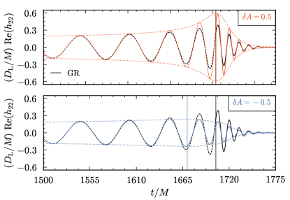
Figure 2: The time evolution near the merger of the real part of the $h_{22}$ mode for nonzero values of the amplitude parameter $\delta A$. We show the GR prediction ($\delta A=0$) with the black lines. Top panel: for $\delta A=0.5$. Bottom panel: for $\delta A=-0.5$. In both panels, we also show $\pm|h_{22}|$ for the non-GR waveform (dotted lines), and we use different line styles for the segment $t\leqslant t^{22}_{\rm match}$ (dashed lines) and $t>t^{22}_{\rm match}$ (solid lines) for all waveform illustrated. The matching times $t^{22}_{\rm match}$ are marked by the vertical lines.

In Fig. 3, we show a “continuum” of waveforms around the time of merger, obtained by finely covering the interval $\delta A\in[-0.5,\,0.5]$, and including $\delta A$ modifications to all modes in pSEOBNRHM. The GR prediction is shown by the black solid line. The top panel shows the real part of the strain, the middle panel the strain amplitude, and the bottom panel the instantaneous frequency, defined as $f=(2\pi)^{-1}\,{\rm d}\,{\rm arg}(h_{+}-{\rm i}h_{\times})/{\rm d}t$. As expected, we see that $f$ does not change by varying $\delta A$, while the middle panel shows clearly how $\delta A$ changes the GW amplitude. For negative values of $\delta A$, the presence of a local minimum in the GW amplitude is evident, as discussed previously.

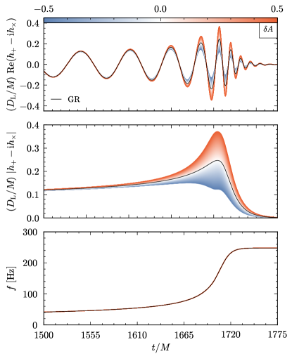
Figure 3: The time evolution near the merger of the GW strain for nonzero values of the amplitude parameter $\delta A$, taken to affect in the same way all the $h_{\ell m}$ modes. The GR prediction ($\delta A=0$) is shown by the black curves. We show the real part of the strain (top panel), the strain amplitude (middle panel), and the instantaneous frequency (bottom panel). As expected, the latter is unaffected by the changes to the peak amplitude of the various GW modes.

III.2 The frequency parameter $\delta\omega$

We now consider $\delta\omega$, the frequency parameter. Figure 4 is analogous to Fig. 2, except that we now consider $\delta\omega=0.5$ (top panel) and $\delta\omega=-0.5$ (bottom panel). We see that $\delta\omega$ induces a time-dependent phase shift to the waveform, with its effects being most noticeable near the merger, and causing $t_{\rm match}$ to happen later (earlier) relative to GR when $\delta\omega>0$ ($\delta\omega<0$), while keeping the peak amplitude unaffected.

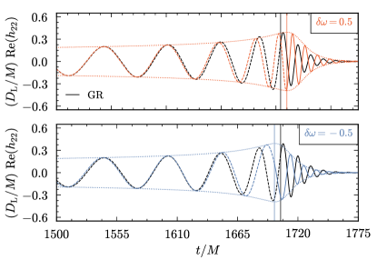
Figure 4: The time evolution near the merger of the real part of the $h_{22}$ mode for nonzero values of the frequency parameter $\delta\omega$. We show the GR prediction ($\delta\omega=0$) with the black lines. Top panel: for $\delta\omega=0.5$. Bottom panel: for $\delta\omega=-0.5$. In both panels, we also show $\pm|h_{22}|$ for the non-GR waveform (dotted lines), and we use different line styles for the segment $t\leqslant t^{22}_{\rm match}$ (dashed lines) and $t>t^{22}_{\rm match}$ (solid lines) for all waveform illustrated. The matching times $t^{22}_{\rm match}$ are marked by the vertical lines.

In Fig. 5, we show an analogous version of Fig. 3, but now for $\delta\omega$. Once more, the top panel shows the real part of the strain, the middle panel the strain amplitude, and the bottom panel the instantaneous frequency. We focus on the region near the merger and we plot the GR curves ($\delta\omega=0$) with black solid lines. In the top panel, we can see the phase differences between the non-GR and GR waveforms, which are the largest around the time of merger and ringdown. This is in part due to the $\delta\omega$ itself, but also to the phase-shift and time-alignment procedure already mentioned, which we perform with respect to the GR waveform. The effect of the latter is small, as can be seen in the middle panel for the amplitude, where all curves nearly overlap in time. In the bottom panel, we note sharp changes to $f$ when $|\delta\omega|\approx 0.5$. They originate from us not imposing the continuity of the time derivative of $\omega_{\ell m}^{\rm NR}$ at $t=t_{\rm match}^{\ell m}$ Bohé et al. (2017); Cotesta et al. (2018).

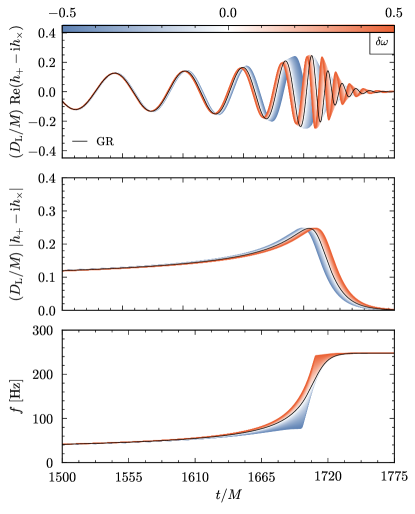
Figure 5: The time evolution near the merger of the GW strain for nonzero values of the frequency parameter $\delta\omega$, assumed to be the same for all $h_{\ell m}$ modes. The GR prediction ($\delta\omega=0$) is shown by the black curves. We show the real part of the strain (top panel), the strain amplitude (middle panel), and the instantaneous frequency (bottom panel). In the top panel, we clearly see the phase difference between the non-GR and GR waveform near the merger. This is partially due to the $\delta\omega$ itself, but also to the phase-shift and time-alignment done with respect to the GR waveform. The effect of the latter is small as can be seen in the middle panel, which shows the amplitude. The sharp changes to $f$ in the bottom panel for $|\delta\omega|\approx 0.5$ originate from us not imposing the continuity of the time derivative of $\omega_{\ell m}^{\rm NR}$ at $t=t_{\rm match}^{\ell m}$.

III.3 The time shift parameter $\delta\Delta t$

Finally, we now consider $\delta\Delta t$, the time shift parameter. In Fig 6, which is analogous to both Figs. 2 and 4, we show waveforms for $\delta\Delta t=0.5$ (top panel) and $\delta\Delta t=-0.5$ (bottom panel). Overall, we see small changes to the GR waveform, in the form of an earlier $t_{\rm match}$ when $\delta\Delta t>0$, and later $t_{\rm match}$ when $\delta\Delta t<0$. Here, the changes due to the phase-shift and time-alignment are negligible, and the shifts seen in the figure are due to $\delta\Delta t$.

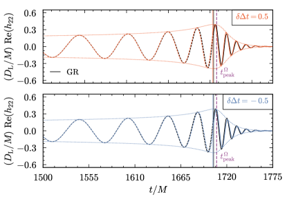
Figure 6: The time evolution near the merger of the real part of the $h_{22}$ mode for nonzero values of the time shift parameter $\delta\Delta t$. We show the GR prediction ($\delta\Delta t=0$) with the black lines. Top panel: for $\delta\Delta t=0.5$. Bottom panel: for $\delta\Delta t=-0.5$. In both panels, we also show $\pm|h_{22}|$ for the non-GR waveform (dotted lines), and we use different line styles for the segment $t\leqslant t^{22}_{\rm match}$ (dashed lines) and $t>t^{22}_{\rm match}$ (solid lines) for all waveform illustrated. The matching times $t^{22}_{\rm match}$ are marked by the vertical lines. For reference, we also show the instant in which the EOB frequency peaks ($t^{\Omega}_{\rm peak}$) with vertical dashed lines.

Finally, in Fig. 7 we show a sequence of waveforms around the time of merger, obtained by finely covering the interval $\delta\Delta t\in[-0.5,\,0.5]$. The GR prediction is shown by the black solid line. We see that the changes to the strain (top panel), its amplitude (middle panel), and its frequency evolution (bottom panel) are small. Therefore, $\delta\Delta t$ introduces changes to the GR waveform which are in general subdominant relative to those due to $\delta A$ and $\delta\omega$. We also remark that $\Delta t^{\rm GR}_{\ell m}$ is not very sensitive to the EOB calibration against NR waveform. Hence, the fractional changes we are introducing on $\Delta t^{\rm GR}_{\ell m}$ are comparable with the NR fitting errors. This explains why this parameter affects the GR waveforms so little.

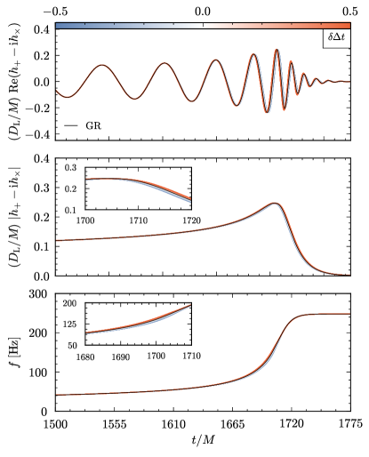
Figure 7: The time evolution near the merger of the GW strain for nonzero values of the time shift parameter $\delta\Delta t$, assumed to be the same for all $h_{\ell m}$ modes. The GR prediction ($\delta\Delta t=0$) is shown by the black curves. We show the real part of the strain (top panel), the strain amplitude (middle panel), and the instantaneous frequency (bottom panel). The insets zoom into the time intervals $t/M\in[1700,\,1720]$ in the middle panel and $t/M\in[1500,\,1775]$ in the bottom panel.

IV Parameter estimation

In the previous section, we have introduced our waveform model and discussed the properties of the waveform morphology. Here, we summarize the Bayesian inference formalism used for parameter estimation of GW signals and synthetic-data studies. We describe the prior choices and the criteria for the GW event selection.

IV.1 Bayesian parameter estimation

Our hypothesis, $\mathcal{H}$, is that in the detector data, $d$, an observed GW signal is described by the waveform model pSEOBNRHM. The model pSEOBNRHM has a set of GR and non-GR parameters, as in Eqs. (1) and (16), where

$$\bm{\vartheta}_{\rm nGR}=\left\{\delta A,\,\delta\omega,\,\delta\Delta t,\,\delta f_{220},\,\delta\tau_{220}\right\}\,.$$ (20)

As said, we assume that the merger modifications are the same for all $(\ell,m)$ modes present in the model pSEOBNRHM.

The posterior probability distribution on the parameters of the model, $\bm{\vartheta}$, given the hypothesis, $\mathcal{H}$, is obtained using Bayes’ theorem,

$$P(\bm{\vartheta}|d,\mathcal{H})=\frac{P(\bm{\vartheta}|\mathcal{H})P(d|\bm{\vartheta},\mathcal{H})}{P(d|\mathcal{H})}\,,$$ (21)

where $P(\bm{\vartheta}|\mathcal{H})$ is the prior probability distribution, $P(d|\bm{\vartheta},\mathcal{H})$ is the likelihood function, and $P(d|\mathcal{H})$ is the evidence of the hypothesis $\mathcal{H}$. For a detector with stationary, Gaussian noise and power spectral density $S_{n}(f)$, the likelihood function can be written as

$$P(d|\bm{\vartheta},\mathcal{H})\propto\exp\left[-\tfrac{1}{2}\left<d-h(\bm{\vartheta})|d-h(\bm{\vartheta})\right>\right]\,,$$ (22)

where the noise-weighted inner product is defined as

$$\langle A|B\rangle=2\int_{f_{\rm low}}^{f_{\rm high}}{\rm d}f\,\frac{\tilde{A}^{*}(f)\tilde{B}(f)+\tilde{A}(f)\tilde{B}^{*}(f)}{S_{n}(f)}\,,$$ (23)

where $\tilde{A}(f)$ is the Fourier transform of $A(t)$, and the asterisk denotes the complex conjugation, and $S_{n}(f)$ is the one-sided power spectral density of the detector. The integration limits $f_{\rm low}$ and $f_{\rm high}$ set the bandwidth of the detector’s sensitivity. We follow the LVK analysis and set $f_{\rm low}=20~{}\text{Hz}$, while $f_{\rm high}$ is the Nyquist frequency Abbott et al. (2021e). The posterior distributions are computed by using LALInferenceMCMC Rover et al. (2006); van der Sluys et al. (2008), a Markov-chain Monte Carlo that uses the Metropolis-Hastings algorithm to survey the likelihood surface and is implemented in LALInference Veitch et al. (2015), part of the LALSuite software suite LIGO Scientific Collaboration (2018).

IV.2 Prior choices

The prior distributions on the GR parameters are assumed to be uniform in the component masses $(m_{1},m_{2})$, uniform and isotropic in the spin magnitudes $(\chi_{1},\chi_{2})$, isotropic on the binary orientation, and isotropically distributed on a sphere for the source location with $P(D_{L})\propto D_{L}^{2}$.

For the non-GR parameters, as explained in Sec. II.2, the internal consistency of the pSEOBNRHM model requires that both $\delta\Delta t$ and $\delta\tau_{220}$ are larger than $-1$ (cf. Table 1). We use this fact to fix a common lower limit on the uniform priors on all $\bm{\vartheta}_{\rm nGR}$. We set $1$ to be an upper limit on the uniform priors on the non-GR parameters. This was sufficient in most of our analysis, but in a few cases we found that the marginalized posteriors distributions for one or more non-GR parameters had support at $\bm{\vartheta}_{\rm nGR}\approx 1$. In such cases we extended the priors’ domains to $\bm{\vartheta}_{\rm nGR}\in(-1,\,+2]$. Even at this wider range, we did not find anomalies in the waveform.

IV.3 Event selection

The pSEOBNRHM ringdown analysis performed in Ref. Abbott et al. (2021b) selected GW events from the GWTC-3 catalog Abbott et al. (2021e) which had a signal-to-noise ratio (SNR) $\geqslant 8$ in the inspiral and post-inspiral regimes. The requirement on the inspiral regime allows one to break the strong degeneracy between the total mass of the binary and the ringdown deviation parameters Brito et al. (2018); Ghosh et al. (2021). Among the GW events that meet this criteria, two stand out in terms of their constraining power on $\bm{\vartheta}_{\rm nGR}^{\rm RD}$, namely GW150914 Abbott et al. (2016b, c) and GW200129_065458 (hereafter GW200129) Abbott et al. (2021e). These two events, with a median total source-frame masses of $64.5~{}{\rm M}_{\odot}$ and $63.4~{}{\rm M}_{\odot}$, respectively, are among the loudest BBH signals to date with a median total network SNR of 26.0 and 26.8, respectively Abbott et al. (2021d, e). GW150914 was detected by the two LIGO detectors at Hanford and Livingston, whereas GW200129 was detected by the three-detector network of LIGO Hanford, Livingston, and Virgo.

We guide ourselves by this result and use these two events to investigate what constraints we can place on the merger-ringdown parameters. We remark that this SNR selection criteria may be too strong if we are interested in $\bm{\vartheta}_{\rm nGR}^{\rm merger}$ only. We leave the study of the optimal SNR to constrain only the merger parameters to a future work.

V Results: synthetic-signal injection studies

Parameter (detector frame)	Value
Primary mass, $m_{1}$ [${\rm M}_{\odot}$]	38.5
Secondary mass, $m_{2}$ [${\rm M}_{\odot}$]	33.4
Primary spin, $\chi_{1}$	$3.47\times 10^{-3}$
Secondary spin, $\chi_{2}$	$-4.40\times 10^{-2}$
Inclination, $\iota$ [rad]	2.69
Polarization, $\psi$ [rad]	1.58
Right ascension, $\alpha$ [rad]	1.22
Declination, $\delta$ [rad]	$-1.46$
Luminosity distance, $D_{\text{L}}$ [Mpc]	337
Reference time, $t_{c}$ [GPS]	1126285216
Reference phase, $\phi_{c}$ [rad]	0.00

Table 2: Values of the parameters $\bm{\vartheta}_{\rm GR}$ used in all synthetic-signal injection studies in Sec. V. The parameters are representative of GW150914, except for the luminosity distance, which is chosen such that the total SNR, in a detector network constituted by LIGO Hanford and Livingston operating at design sensitivity, is approximately 100.

In this section, we use pSEOBNRHM to perform a number of synthetic-signal injection studies. As we saw in Sec. II, pSEOBNRHM is a smooth deformation of the GR waveform model SEOBNRHM, which is recovered when all $\bm{\vartheta}_{\rm nGR}$ parameters are set to zero. This allows us to explore different scenarios that differ from one another on whether the GW signal and the GW model used to infer the parameters of this signal are described by GR ($\bm{\vartheta}_{\rm nGR}=0$) or not ($\bm{\vartheta}_{\rm nGR}\neq 0$). We summarize these possibilities in Table 3.

To prepare the GW signal we need to fix $\bm{\vartheta}=\bm{\vartheta}_{\rm GR}\cup\bm{\vartheta}_{\rm nGR}$. In all cases, we use values of $\bm{\vartheta}_{\rm GR}$ illustrative of a GW150914-like BBH as in Table 2. We set all non-GR parameters to the same value, $\bm{\vartheta}_{\rm nGR}=0.1$, whenever the injected signal is non-GR. By working exclusively with the pSEOBNRHM waveform model, we avoid introducing systematic errors due to waveform modeling in our analysis. We also employ an averaged (zero-noise) realization of the noise to avoid statistical errors due to noise. The resulting GW signal is then analyzed with the power spectral density $S_{n}(f)$ of the LIGO Hanford and Livingston detectors both at design sensitivity Barsotti et al. (2018). In all cases, we set the distance to the binary to be such that the total network SNR is approximately $100$.

In Sec. V.1, we do a preliminary analysis where both injected and model waveforms are described by GR. This allows us to access the accuracy with which different binary parameters can be recovered from the data in the detector network. With these results as a benchmark, we can then proceed to inject a non-GR waveform and analyze it with a GR model. This allows us to study the systematic error introduced on the inferred binary parameters by assuming a priori that GR is true, while nature may not be so (the so-called fundamental bias). In Sec. V.2, we inject a GR waveform and try to recover its parameters with a non-GR model. This allows us to answer how much the non-GR parameters can be constrained given an event consistent with GR. Finally, in Sec. V.3, we use non-GR waveforms as both our injection and our model. This answers whether we can detect the presence of the non-GR parameters in our signal.

		Model
		GR	non-GR
Injection	GR	Sec. V.1	Sec. V.2
	non-GR	Sec. V.1	Sec. V.3

Table 3: Summary of the synthetic-signal injection simulations performed in Sec. V. The label “GR ” refers to the SEOBNRHM waveform model, whereas the label “non-GR” refers to the pSEOBNRHM waveform model, where all merger-ringdown parameters are set deviate in $10\%$ deviations relative to their corresponding GR values.

V.1 Fundamental biases on binary parameters

We first explore the presence (or not) of biases in the inference of binary parameters when the template waveform model assumes GR, while the injected GW signal is non-GR Yunes and Pretorius (2009); Vallisneri and Yunes (2013). For this purpose, we first inject a synthetic GR GW signal with $\text{SNR}=98$ and recover the binary parameters with a GR model. By doing this exercise first, we gain an idea on the accuracy with which the parameters of the binary (cf. Table 2) can be recovered in our set up. Next, we repeat the same analysis but now using as our synthetic GW signal the one obtained with pSEOBNRHM. The signal is prepared using the same binary parameters $\bm{\vartheta}_{\rm GR}$ shown in Table 2 with $\text{SNR}=104$, but now we let $\bm{\vartheta}_{\rm nGR}=0.1$.

The results of our two analyses are shown in Fig. 8. We show the one- and two-dimensional posterior distributions of a subset of the intrinsic binary parameters, namely, the mass ratio $q$, the detector-frame chirp mass $\mathcal{M}$ and the effective spin $\chi_{\rm eff}$. In all panels, the “true” (injection) values of these parameters are marked by the vertical and horizon lines. We see that in the case of a non-GR injection (solid curves), the posterior distributions of the parameters are shifted from the injected values and from the posterior distributions in the case of a GR injection (dashed curves). We attribute the differences in the 90% contours of the posterior distributions to the fact that in the non-GR injection a smaller value of the chirp mass ${\cal M}$ is inferred. This suggests that the GR waveform that best fits the data has a longer inspiral and this makes the inference of the other binary parameters more precise. The recovered SNR from the GR analysis of the non-GR signal is almost the same as the injected one, i.e., $\text{SNR}=104$. Hence, if a GW signal with deviations from GR would be analyzed by current GR templates, the GW event would be interpreted as a BBH in GR with different values of the binary parameters.

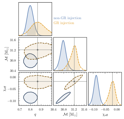
Figure 8: The one- and two-dimensional posterior distributions on the intrinsic binary parameters of mass ratio $q$, detector-frame chirp mass $\mathcal{M}$ and effective spin $\chi_{\rm eff}$ for a GR injection (dashed curve) and a non-GR injection (solid curve) with $10\%$ deviations in the merger-ringdown parameters $\bm{\vartheta}_{\rm nGR}$. All contours indicate 90% credible regions. The parameter estimation is performed assuming the GR SEOBNRHM waveform model. The vertical and horizontal lines mark the injected values. The measurements with non-GR injections are visibly biased, most preeminently in $\chi_{\rm eff}$ and $\mathcal{M}$.

V.2 Constraints on deviations to general relativity

We now inject a synthetic GW signal in GR using the parameters $\bm{\vartheta}_{\rm GR}$ in Table 2 with $\text{SNR}=98$. We analyze the signal using the pSEOBNRHM waveform model, allowing both $\bm{\vartheta}_{\rm GR}$ in Eq. (1) and $\bm{\vartheta}_{\rm nGR}$ in Eq. (20) to vary. This simulates a scenario where we have a GW event consistent with GR and we want to understand which constraints it places on the non-GR parameters in our waveform model.

We summarize the results of the analysis in Fig. 9, where we show the one- and two-dimensional posterior probability distributions of the merger-ringdown parameters $\bm{\vartheta}_{\rm nGR}$. We find that the marginalized posterior distributions of the non-GR parameters are consistent with the corresponding injected values in GR, which are indicated by the markers. We can infer that a GW150914-like event with $\text{SNR}=98$ would constrain the deformation parameters in the range between 5% (for $\delta A$ and $\delta f_{220}$) and 20% (for $\delta\tau_{220}$) at 90% credible level. In Appendix A, Fig. 15, we show the posterior distributions on the intrinsic binary parameters.

The best constrained parameter is the amplitude, $\delta A$, whereas the less constrained parameter is the time shift, $\delta\Delta t$. For the latter, we obtain a posterior distribution that has support onto a wide range of the prior. This is perhaps unsurprising due to the small deviations caused by $\delta\Delta t$ in the waveform in comparison with $\delta\omega$ (compare Figs. 4 and 6). We also observe a negative correlation between these two parameters and hence increasing precision on one is likely to increase uncertainty on the other; see the $\delta\Delta t$–$\delta\omega$ panel in Fig. 9. Together, these results suggest that considering $\delta A$ and $\delta\omega$ is sufficient, if one is interested in doing a test of GR only in the plunge-merger stage of the binary’s coalescence.

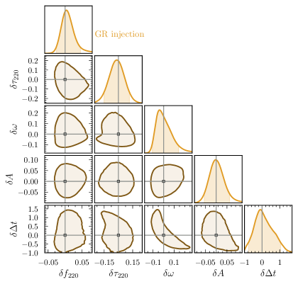
Figure 9: The one- and two-dimensional posterior distributions on the merger-ringdown parameters $\bm{\vartheta}_{\rm nGR}$. All contours indicate 90% credible regions. We considered a GR injection and recovered with the pSEOBNRHM model. The vertical and horizontal lines mark the injected values for the deviation parameters, i.e., $\bm{\vartheta}_{\rm nGR}=0$. The inferred values on $\bm{\vartheta}_{\rm nGR}$ are consistent with the zero, and their width of the marginalized posterior distribution inform us with which accuracy we may constrain these parameters.

V.3 Detecting deviations from general relativity

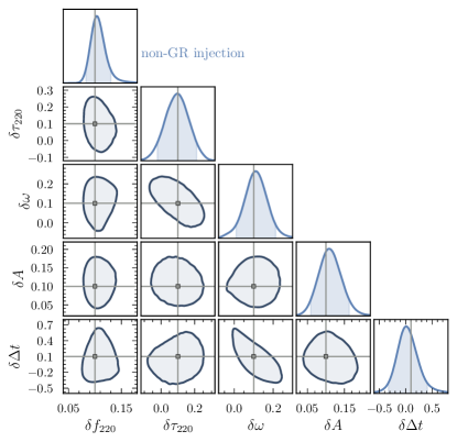
Figure 10: The one- and two-dimensional posterior distributions on the merger-ringdown parameters $\bm{\vartheta}_{\rm nGR}$. All contours correspond to 90% credible regions. In comparison to Fig. 9, this time we use pSEOBNRHM prepare the injection. This allow us to understand how well we can measure the non-GR parameters. The vertical and horizontal lines mark the injected values for the deviation parameters, i.e., $\bm{\vartheta}_{\rm nGR}=0.1$. The marginalized posterior distributions on $\bm{\vartheta}_{\rm nGR}$ are consistent with their injection values.

We now study whether we can detect the presence of the non-GR parameters. To do so, we inject a synthetic GW signal where the binary parameters are shown in Table 2, $\text{SNR}=104$, and we set the merger-ringdown parameters to be $10\%$ larger than their corresponding GR values.

We summarize the outcome of our parameter estimation in Fig. 10, where we show the one- and two-dimensional posterior distributions for the $\bm{\vartheta}_{\rm nGR}$ parameters. We see that all posteriors are consistent with the injected values, indicated by the markers. Moreover, the posteriors for $\bm{\vartheta}_{\rm nGR}$ have support at their null, GR value. The exceptions are the amplitude $\delta A$ and the QNM frequency $\delta f_{220}$ parameters, which have no support at their GR values at 90% credible level. This suggests that these two parameters are the most promising ones in signaling the presence of beyond-GR physics for GW150914-like binaries. In fact, we will see this suggestion taking place in our analysis of GW200129 in Sec. VII.

VI Analysis of GW150914: constraints on the plunge-merger-ringdown parameters

Having gained some intuition on the role of the merger-ringdown parameters in the synthetic-signal injections presented in Sec. V, we now apply the pSEOBNRHM model to the analysis of real GW events. Our analysis, here and in Sec. VII, uses the power spectral density of the detectors from the Gravitational Wave Open Science Center (GWOSC) Abbott et al. (2021g), and calibration envelopes as used for the analyses in Ref. Abbott et al. (2021b). We will start with GW1501914, the first GW event observed by the LIGO-Virgo Collaboration Abbott et al. (2016b).

We will focus our analysis to two subsets of merger-ringdown parameters due to the smaller SNR of this event (and of GW200129) in comparison to the SNR $\approx 100$ scenarios studied in the previous section. First, we have seen that the time-shift parameter $\delta\Delta t$ is the hardest parameter to constrain, and that it has wide posteriors even at such large SNRs. This motivates us to consider, among the merger parameters, only

$$\bm{\vartheta}_{\rm nGR}=\{\delta A,\,\delta\omega\}\,,$$ (24)

to perform a “merger test of GR”. Second, we performed a parameter estimation of GW150914, using all $\bm{\vartheta}_{\rm nGR}$ parameters in Eq. (20). We found correlations between the frequency parameter $\delta\omega$ and the QNM deformations parameters $\delta f_{220}$ and $\delta\tau_{220}$. Moreover, we also did a series of synthetic-signal injection studies using the binary parameters listed in Table 2, with SNR$=26$, and in Gaussian noise. In some of these cases, we also found correlations between $\delta\omega$ and $\delta f_{220}$ and $\delta\tau_{220}$.

In summary, these correlations arise either when the GW event has low SNR or due to noise. This suggest using

$$\bm{\vartheta}_{\rm nGR}=\{\delta A,\,\delta f_{220},\,\delta\tau_{220}\}\,,$$ (25)

to perform a “merger-ringdown test of GR”.

In Fig. 11 we show the results of our merger test of GR. The corner plot shows the one- and two-dimensional posterior probability distributions of $\delta A$ and $\delta\omega$. The posterior distributions are consistent with the null value predicted in GR. We obtain from GW150914,

$$\delta A=-0.01^{+0.27}_{-0.19}\,,\quad\textrm{and}\quad\delta\omega=0.00^{+0.17}_{-0.12}\,,$$ (26)

at 90% credible level. This shows that we already constrain deviations from GR around the merger time of BBH coalescences to about 20% with present GW events.

Figure 12 is a similar plot, but for the merger-ringdown test of GR. Once more, we find that the inferred values of the non-GR parameters are consistent with GR,

$$\delta A=0.03^{+0.29}_{-0.20}\,,\,\delta f_{220}=0.041^{+0.151}_{-0.084}\,,\,\delta\tau_{220}=0.04^{+0.27}_{-0.29}\,,\,$$

at 90% credible level. The bound on the amplitude parameter is similar to the one obtained in the merger test, shown in Eq. (26). Also, the bounds on the ringdown parameters are similar to those obtain in Ref. Ghosh et al. (2021) ($\delta f_{220}=0.05^{+0.11}_{-0.07}$ and $\delta\tau_{220}=-0.07^{+0.26}_{-0.23}$), which had only these two quantities as its non-GR parameters. In Appendix A, Fig. 16, we show the posterior distributions on the intrinsic binary parameters for both tests of GR.

When interpreting our inferences on these parameters, it is important to note that the statistical error in our analysis ($\approx 20\%$) is larger than the systematic error due to fitting $|h_{{\ell m}}^{\rm NR}|$ and $\omega_{{\ell m}}^{\rm NR}$ against NR data, which is at most around $4\%$ with current models Bohé et al. (2017); Cotesta et al. (2018), depending on where one is in the $\eta$–$\chi_{\rm eff}$ parameter space. In fact, we see that the median values of $\delta A$ and $\delta\omega$ fall within this fitting error. In conclusion, we can claim to have placed a constraint on these non-GR parameters with GW150914.

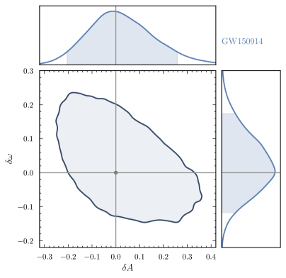
Figure 11: The one- and two-dimensional posterior distributions on $\delta A$ and $\delta\omega$ obtained by analyzing GW150914. All contours correspond to 90% credible regions. The marginalized posterior distributions are consistent with GR, i.e., $\delta A=\delta\omega=0$, identified in the plot with the horizontal and vertical lines. We found that $\delta A=-0.01^{+0.27}_{-0.19}$ and $\delta\omega=0.00^{+0.17}_{-0.12}$ at 90% credible level.

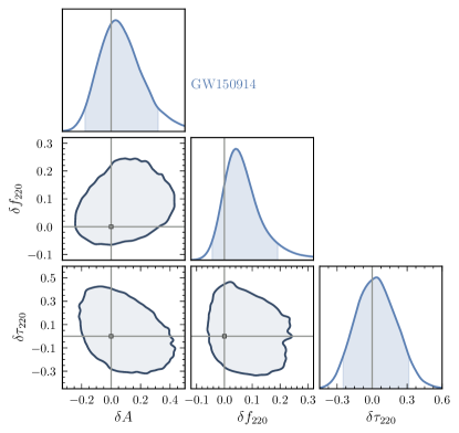
Figure 12: The one- and two-dimensional posterior distributions on the merger parameter $\delta A$, and ringdown parameters $\delta f_{220}$ and $\delta\tau_{220}$, obtained by analyzing GW150914. The marginalized posterior distributions are consistent with GR, i.e., $\delta A=\delta f_{220}=\delta\omega_{220}=0$, identified in the plot with the horizontal and vertical lines. We found that GW150914 constrains these parameters to be $\delta A=0.03^{+0.29}_{-0.20}$, $\delta f_{220}=0.041^{+0.151}_{-0.084}$, and $\delta\tau_{220}=0.04^{+0.27}_{-0.29}$ at 90% credible level.

VII The case of GW200129: the importance of waveform systematics and data-quality in tests of general relativity

We now turn our attention to GW200129 and, following what we have learned in the previous section, we first consider pSEOBNRHM with only $\delta A$ and $\delta\omega$ as non-GR parameters. We show the one- and two-dimensional marginalized posteriors of these parameters with the black solid curves in the left panel of Fig. 13. We see that while our inferred value of $\delta\omega$ ($\delta\omega=-0.002^{+0.097}_{-0.082}$ at the 90% credible level) is consistent with GR, our inferred value of $\delta A$ ($\delta A=0.44^{+0.38}_{-0.28}$ at the 90% credible level) exhibits a gross violation of GR.

Have we found a strong evidence of violation of GR in GW200129? Assuming that this is not the case, the apparent violation of GR could be either due to statistical errors or to systematic errors. To explore the first possibility, we perform a series of synthetic-data injection studies. As our first step, we do a parameter-estimation study in zero noise, where the injected GW signal is generated with SEOBNRHM and we use the binary parameters corresponding to the maximum likelihood point from the GWTC-3 data release by the LVK Collaboration et al. (2021) analysis of GW200129. The LVK analysis was done separately with two quasicircular and spin-precessing waveform models, SEOBNRv4PHM Ossokine et al. (2020) and IMRPhenomXPHM Pratten et al. (2021), employing different parameter estimation libraries, RIFT Pankow et al. (2015); Lange et al. (2017); Wysocki et al. (2019) and Bilby Ashton et al. (2019); Romero-Shaw et al. (2020), respectively. Here, as a reference, we use the maximum likelihood point of the analysis that employed the IMRPhenomXPHM model, and we expect the results to be qualitatively similar had we used SEOBNRv4PHM. More specifically, because the SEOBNRHM model we are using is nonprecessing, we use only the masses and luminosity distance from the maximum-likelihood point.

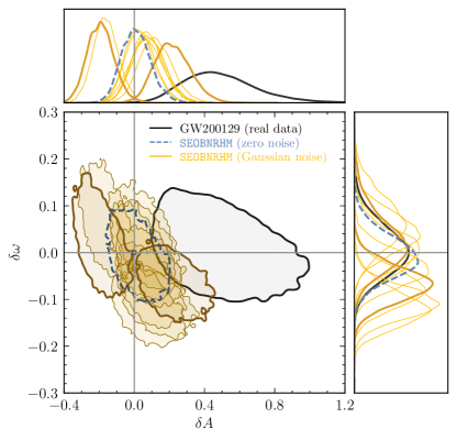
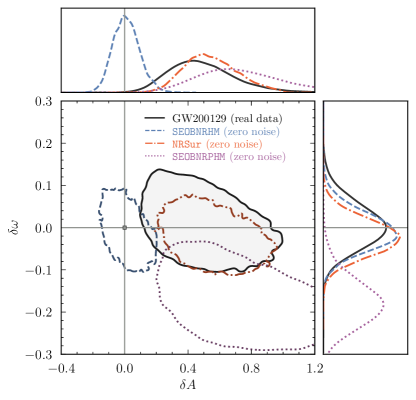
Figure 13: Corner plots showing the one- and two-dimensional posterior distribution functions for $\delta A$ and $\delta\omega$ for our studies of GW200129 and GW200129-like BBHs. All contours indicate 90% credible regions. Left panel: results of our reanalysis of GW200129 data with pSEOBNRHM (black solid curves) and for a GW200129-like injection generated with SEOBNRHM. For the latter, we used the maximum-likelihood point of LVK’s original analysis of GW200129 which employed the IMRPhenomXPHM model to generate the synthetic GW signal. We performed the parameter estimation of these injections in zero noise (dashed curves) and in ten Gaussian noise realizations (yellow solid curves). Right panel: Similar, but having generated two additional GW200129-like synthetic signals with NRSur7dq4 (dot-dashed curves) and with SEOBNRv4PHM (dotted curves). Both models include spin precession effects. Observe how the posteriors distributions are in tension with GR [marker at $(\delta A,\,\delta\omega)=(0,\,0)$] when we include spin-precession effects in the synthetic data and we recover with a nonprecessing and non-GR waveform model.

The resultant posterior distributions are shown in the left panel of Fig. 13 (dashed curves) and they are, reassuringly, consistent with GR. We also repeat this analysis for ten Gaussian noise realizations, using the same synthetic GW signal (yellow solid curves in the left panel of Fig. 13). Consistent with the expectations, two noise realizations yield marginalized posteriors on $\delta\omega$ and $\delta A$ which are not consistent with GR at 90% credible level (shown by the thicker yellow solid curves). It is worth observing how the Gaussian noise curves have qualitatively the same shapes (spreads), with the two outliers being shifted away from $(\delta A,\,\delta\omega)=(0,\,0)$. This is an expected behavior consistent with the stationary, Gaussian assumption of statistical noise. These results, hence, disfavor the possibility that the violations of GR we are observing are due to Gaussian noise or due to the particular binary parameters inferred for this event. The latter alternative would have been quite unlikely in the first place, because both GW200129 and GW150914 have similar binary parameters and SNRs, and we have already found that GW1501914 is consistent with GR in Sec. VI (cf. Fig. 11).

As our next step, we perform two additional parameter estimation runs, in zero noise, but now generating our synthetic GW signal with the SEOBNRv4PHM Ossokine et al. (2020) and the NRSur7dq4 Varma et al. (2019); Field et al. (2022) waveform models. Both models allow for spin precession, unlike our pSEOBNRHM. Hence, we can study if the GR deviations we are finding are due to systematic errors in the GW modeling. Once again, the maximum-likelihood point of the LVK analysis of GW200129 using IMRPhenomXPHM was used, but this time with the binary in-plane spin components included. We show our results in the right panel of Fig. 13. The one- and two-dimensional posterior distributions of $\delta\omega$ and $\delta A$ are shown in dash-dotted curves for the NRSur7dq4 injection and with dotted curves for the SEOBNRv4PHM injection. For reference, we also include the posterior distribution associated to the SEOBNRHM injection (dashed curves) and to the data from GW200129 (solid curves). We see that these two spin-precessing GW signals, when analyzed in zero noise, are also in disagreement with GR, when analyzed with our nonprecessing non-GR model. We also see that our results using NRSur7dq4 (which compares the best against NR simulations in its regime of validity) are in good agreement with what we obtain by analyzing the GW200129 data. These results, compared with those obtained from the SEOBNRHM injection, suggest that the presence of spin precession in the GR signal, biases us to find a false evidence for beyond-GR effects when we use a nonprecessing non-GR model.

Is this the full story? In Ref. Payne et al. (2022), Payne et al. revisited the evidence of spin precession in GW200129 Hannam et al. (2022). They concluded that the evidence for spin-precession originates from the LIGO Livingston data, in the 20–50 Hz frequency range, alone. This range coincides with the frequency range that displays data quality issues, due to a glitch in the detector that overlapped in time with the signal Abbott et al. (2021e). By reanalyzing the GW200129 data with $f_{\rm low}>50$ Hz (while leaving LIGO Hanford data intact and not using Virgo data), they showed that the evidence in favor of spin precession in this event disappears. See Ref. Payne et al. (2022) for a detailed discussion. Moreover, a reanalysis of the LIGO Livingston glitch mitigation showed that the difference between the spin-precessing and nonprecessing interpretations of this event is subdominant relative to uncertainties in the glitch subtraction Payne et al. (2022). Since we have used the glitch-subtracted data in our parameter estimation, we are then led to the second conclusion of our study of this event, namely that: issues with data quality can introduce biases in non-GR parameters, to an extent that one can find significant false violations of GR in GW events detected with present GW observatories. See Ref. Kwok et al. (2022) for a recent study of this issue.

Furthermore, we repeat here the analysis we have performed for GW150914 where we considered $\bm{\vartheta}_{\rm nGR}=\{\delta A,\,\delta f_{220},\,\delta\tau_{220}\}$ as our non-GR parameters. For the discussion that follows, we assume that GW200129 is an unmistakable genuine spin-precessing BBH. We show our results in Fig. 14. We see that while our inferred values of $\delta f_{220}$ and $\delta\tau_{220}$ are consistent with GR at 90% confidence level, our inference of the amplitude parameter, $\delta A=0.50^{+0.46}_{-0.30}$ at 90% credible level, remains inconsistent with GR. Moreover, this value hardly changes from our $\{\delta A,\,\delta\omega\}$-study, i.e., $\delta A=0.44^{+0.38}_{-0.28}$, at the same credible level.

This result is interesting for two reasons. First, it indicates that the systematic error caused by spin-precession mismodeling is robust to the inclusion of deformations to the ringdown QNM frequencies, at least for this event. Second, there is a commonality between our finding for GW150914 (see Fig. 12) and GW200129 (see Fig. 14) namely, that in both cases the posterior distributions of $\delta f_{220}$ and $\delta\tau_{220}$ are consistent with GR, despite the larger parameter space due to the inclusion of $\delta A$. In the case in which one considers only $\delta f_{220}$ and $\delta\tau_{220}$ as non-GR parameter, the consistency with GR had already been established in Ref. Ghosh et al. (2021), and in particular in Ref. Abbott et al. (2021b); see Sec. VIII, Fig. 14 there. Our analysis of these two GW events with the new pSEOBNRHM waveform model suggests the following: the model would be able to detect deviations from nonprecessing quasicircular GW signals in the plunge-merger-ringdown which otherwise would not be seen when having deformations to the ringdown only.

We close our discussion of GW200129 with two remarks. First, data-quality issues aside, we can think of our spin-precessing injection studies as illustrative of what could happen in upcoming LVK observation runs. By doing so, we have then demonstrated the existence of a systematic error on the non-GR parameters caused by spin-precession mismodeling. Second, although we have proposed pSEOBNRHM as a means of constraining (or detecting) potential non-GR physics in BBH coalescences, we can also interpret the merger parameters as indicators of our ignorance in GR waveform modeling. More concretely, in a hypothetical scenario where GW modelers did not know that BBH can spin precess, an analysis of GW200129 with pSEOBNRHM would suggest that their model of the peak GW-mode amplitudes is insufficient to describe this event and hence be an indicative of new, nonmodeled binary dynamics that was absent in their waveform model. They would not be able to say that spin precession is the missing dynamics, but they would at least realize that something is missing.

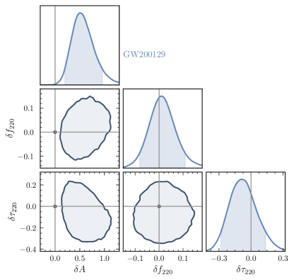
Figure 14: The one- and two-dimensional posterior distribution functions for $\delta A$, $\delta f_{220}$, and $\delta\tau_{220}$ for GW200129. All contours indicate 90% credible regions. We see that while our inferred values for $\delta f_{220}$ and $\delta\tau_{220}$ are consistent with GR, $\delta A$ is not.

VIII Discussions and final remarks

We presented a time-domain IMR waveform model that accommodates parametrized deviations from GR in the plunge-merger-ringdown stage of nonprecessing and quasicircular BBHs. This model generalizes the previous iterations of the pSEOBNRHM model Brito et al. (2018); Ghosh et al. (2021); Mehta et al. (2023), which included deviations from GR in the inspiral phase or modified the QNM frequencies only, by introducing deformations parameters $\bm{\vartheta}^{\rm merger}_{\rm nGR}$ that, for each GW mode, can change the time at which the GW mode peaks, the mode frequency at this instant, and the peak mode amplitude. This new version of pSEOBNRHM reduces to the state-of-the-art SEOBNRHM model Bohé et al. (2017); Cotesta et al. (2018); Mihaylov et al. (2021) for nonprecessing and quasicircular BBHs in the limit in which all deformations parameters are set to zero.

We used pSEOBNRHM to perform a series of injections studies for GW150914-like events exploring (i) the constraints that one could place on these non-GR parameters, (ii) the biases introduced on the intrinsic binary parameters in case nature is not described by GR and we model the signal with a GR template, and, finally, (iii) we studied the measurability of these non-GR parameters.

We also used pSEOBNRHM in a reanalysis of GW150914 and GW200129. For GW150914, we found that the deviations from the GR peak amplitude and the instantaneous GW frequency can already be constrained to about $20\%$ at 90% credible level. For GW200129, we found an interesting interplay between spin precession and false violations of GR that manifests as a $\sim 2\sigma$ deviation from GR in the peak amplitude parameter. By interpreting the evidence for spin precession in this event as due to data-quality issues in the LIGO Livingston detector Payne et al. (2022); Abbott et al. (2021e), we found a further a connection between data-quality issues and false violations of GR Kwok et al. (2022).

These results warrant further studies on the systematic bias due to spin precession in tests of GR. In the context of plunge-merger-ringdown test, this could be achieved by extending the SEOBNRv4PHM waveform model Ossokine et al. (2020) to include the same set of non-GR parameters $\bm{\vartheta}_{\rm nGR}$ used here. It is also natural to explore which systematic effects higher GW modes Pang et al. (2018) and binary eccentricity can introduce in tests of GR. For the latter, see Ref. Bhat et al. (2023) for work in this direction for IMR consistency tests Hughes and Menou (2005); Ghosh et al. (2016) and Ref. Saini et al. (2022) in the context of deviations in the post-Newtonian (PN) GW phasing Yunes and Pretorius (2009); Cornish et al. (2011); Agathos et al. (2014). It would also be interesting to investigate these issues in the context of the ringdown test within the EOB framework employed by LVK Collaboration Abbott et al. (2021b) and which relies on pSEOBNRHM Brito et al. (2018); Ghosh et al. (2021). This could be done by adding non-GR deformations to the SEOBNRv4EHM waveform model of Ref. Ramos-Buades et al. (2022). It would also be important to investigate whether pSEOBNRHM can be used to detect signatures of non-GR physics, as predicted by the rapidly growing field of NR in modified gravity theories (see e.g., Refs. Witek et al. (2019); Okounkova et al. (2017, 2019, 2020); Okounkova (2020); Okounkova et al. (2023); East and Ripley (2021a); Figueras and França (2022); Aresté Saló et al. (2022); Corman et al. (2023)); some of which predict nonperturbative departures from GR only in late-inspiral and merger ringdown Silva et al. (2021); East and Ripley (2021b); Doneva et al. (2022); Elley et al. (2022). One could also study what the theory-agnostic bounds we obtained with GW150914 on the amplitude and GW frequency imply to the free parameters of various modified gravity theories.

The deformations parameters $\bm{\vartheta}^{\rm merger}_{\rm nGR}$ in our pSEOBNRHM model should have an approximate correspondence to the phenomenological deviation parameters (from NR calibrated values) in the “intermediate region” of the IMRPhenom waveform model used in the TIGER pipeline Li et al. (2012); Agathos et al. (2014); Meidam et al. (2018) of the LVK Collaboration Abbott et al. (2016a, 2019a, 2019b, 2021a). Such a mapping could be derived through synthetic injection studies. This work only introduced non-GR parameters in the EOB GW modes and only during the plunge-merger-ringdown. Importantly, and more consistently, in the near future we will extend the parametrization to the EOB conservative and dissipative dynamics.

The interplay between GW waveform systematics, characterization and subtraction of nontransient Gaussian noises in GW detectors, and non-GR physics will become increasingly important in the future. Planned ground-based Punturo et al. (2010); Reitze et al. (2019) and space-borne GW observatories Amaro-Seoane et al. (2017) will detect GW transients with SNRs that may reach the thousands depending on the source. Having all these aspects under control is a daunting task that will need to be faced if one wants to confidently answer the question “Is Einstein still right?” Will and Yunes (2020) in the stage of BBH coalescences where his theory unveils its most outlandish aspects.

Appendix A Estimation of the intrinsic binary parameters

In this Appendix, we compare the posterior distributions on the intrinsic binary parameters obtained using the SEOBNRHM and pSEOBNRHM waveform models. This complements the results shown in Sec. V.2 (Fig. 15) and Sec. VI (Fig. 16). For simplicity, we focus on the total mass $M$, the mass ratio $q$, the effective spin $\chi_{\rm eff}$ and the luminosity distance $D_{\rm L}$.

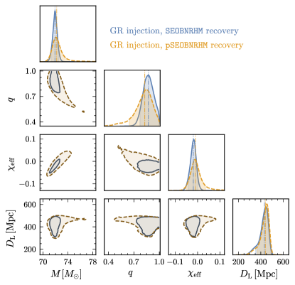
Figure 15: The one- and two-dimensional posterior distributions on the intrinsic binary parameters of the total mas $M$, the mass ratio $q$, the effective spin $\chi_{\rm eff}$ and the luminosity distance $D_{\rm L}$ for a GR injection with the parameters in Table 2. The parameter estimation is performed using SEOBNRHM (solid curves) and pSEOBNRHM (dashed curves) waveform models. All contours indicate 90% credible regions and the vertical lines mark the inferred median values for each parameter.

Figure 15 shows the posterior distributions on the intrinsic binary parameters for a GR signal with the properties shown in Table 2. The solid curves are obtained when the parameter estimation is performed with the GR waveform model SEOBNRHM, whereas the dashed curves are obtained with the parametrized plunge-merger-ringdown waveform model pSEOBNRHM (cf. Sec. V.2). In both cases, the SNR is 98. We see that the 90% confidence intervals of the posterior distributions in the two analyses overlap in the parameter space. The most important difference is that the 90% credible intervals are wider in the pSEOBNRHM analysis. There are also changes to the median values of the binary parameters, as can be seen through the vertical lines in the plot.

To be more precise, the posteriors of the pSEOBNRHM model have a tail, most evidently in the mass ratio $q$. For the mass ratio, at 90% confidence interval, we find $q=0.87^{+0.12}_{-0.10}$ (for the SEOBNRHM recovery) and $q=0.84^{+0.15}_{-0.20}$ (for the pSEOBNRHM recovery). The broader posteriors, and tails, are due to the fact that the pSEOBNRHM model has five additional parameters with respect to SEOBNRHM. Qualitatively, by increasing the number of parameters in the model we increase the number of possible waveforms that match, to some extent, the injected signal. This will be most evidently seen in Fig. 16 which we discuss below.

Figure 16 shows the posterior distributions on the intrinsic binary parameters for our analyses of GW150914 (cf. Sec. VI). The solid curves are obtained when we use SEOBNRHM for parameter estimation, whereas the dashed and dotted curves are obtained when we use pSEOBNRHM with non-GR parameters $\{\delta A,\delta\omega\}$ (“merger test of GR”) and $\{\delta A,\delta f_{220},\delta\tau_{220}\}$ (“merger-ringdown test of GR”), respectively. The figure is similar to Fig. 15, discussed above. Again, we see that the 90% confidence intervals of the posterior distributions in the three analyses overlap in the parameter space. However, here we can see more explicitly how the increase of extra non-GR parameters in the waveform model

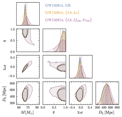
Figure 16: The one- and two-dimensional posterior distributions on the intrinsic binary parameters of the total mass $M$, the mass ratio $q$, the effective spin $\chi_{\rm eff}$ and the luminosity distance $D_{\rm L}$ for GW150914. The parameter estimation is done with SEOBNRHM (solid curves) and pSEOBNRHM waveform model with non-GR parameters $\{\delta A,\delta\omega\}$ (dashed curves) and $\{\delta A,\delta f_{220},\delta\tau_{220}\}$ (dotted curves). All contours indicate 90% credible regions and the vertical lines mark the inferred median values for each parameter.

References

- Will (2014) C. M. Will, “The Confrontation between General Relativity and Experiment,” Living Rev. Rel. 17, 4 (2014), arXiv:1403.7377 [gr-qc] .
- Clifton et al. (2012) T. Clifton, P. G. Ferreira, A. Padilla, and C. Skordis, “Modified Gravity and Cosmology,” Phys. Rept. 513, 1–189 (2012), arXiv:1106.2476 [astro-ph.CO] .
- Kapner et al. (2007) D. J. Kapner, T. S. Cook, E. G. Adelberger, J. H. Gundlach, B. R. Heckel, C. D. Hoyle, and H. E. Swanson, “Tests of the gravitational inverse-square law below the dark-energy length scale,” Phys. Rev. Lett. 98, 021101 (2007), arXiv:hep-ph/0611184 .
- Lee et al. (2020) J. G. Lee, E. G. Adelberger, T. S. Cook, S. M. Fleischer, and B. R. Heckel, “New Test of the Gravitational Law at Separations down to 52 m,” Phys. Rev. Lett. 124, 101101 (2020), arXiv:2002.11761 [hep-ex] .
- Abuter et al. (2020) R. Abuter et al. (GRAVITY), “Detection of the Schwarzschild precession in the orbit of the star S2 near the Galactic centre massive black hole,” Astron. Astrophys. 636, L5 (2020), arXiv:2004.07187 [astro-ph.GA] .
- Kramer et al. (2021) M. Kramer et al., “Strong-Field Gravity Tests with the Double Pulsar,” Phys. Rev. X 11, 041050 (2021), arXiv:2112.06795 [astro-ph.HE] .
- Akiyama et al. (2019) K. Akiyama et al. (Event Horizon Telescope), “First M87 Event Horizon Telescope Results. V. Physical Origin of the Asymmetric Ring,” Astrophys. J. Lett. 875, L5 (2019), arXiv:1906.11242 [astro-ph.GA] .
- Akiyama et al. (2022) K. Akiyama et al. (Event Horizon Telescope), “First Sagittarius A* Event Horizon Telescope Results. VI. Testing the Black Hole Metric,” Astrophys. J. Lett. 930, L17 (2022).
- Abbott et al. (2016a) B. P. Abbott et al. (LIGO Scientific, Virgo), “Tests of general relativity with GW150914,” Phys. Rev. Lett. 116, 221101 (2016a), [Erratum: Phys. Rev. Lett.121,no.12,129902(2018)], arXiv:1602.03841 [gr-qc] .
- Abbott et al. (2019a) B. P. Abbott et al. (LIGO Scientific, Virgo), “Tests of General Relativity with GW170817,” Phys. Rev. Lett. 123, 011102 (2019a), arXiv:1811.00364 [gr-qc] .
- Abbott et al. (2019b) B. P. Abbott et al. (LIGO Scientific, Virgo), “Tests of General Relativity with the Binary Black Hole Signals from the LIGO-Virgo Catalog GWTC-1,” Phys. Rev. D 100, 104036 (2019b), arXiv:1903.04467 [gr-qc] .
- Abbott et al. (2021a) R. Abbott et al. (LIGO Scientific, Virgo), “Tests of general relativity with binary black holes from the second LIGO-Virgo gravitational-wave transient catalog,” Phys. Rev. D 103, 122002 (2021a), arXiv:2010.14529 [gr-qc] .
- Abbott et al. (2021b) R. Abbott et al. (LIGO Scientific, VIRGO, KAGRA), “Tests of General Relativity with GWTC-3,” (2021b), arXiv:2112.06861 [gr-qc] .
- Abbott et al. (2016b) B. P. Abbott et al. (LIGO Scientific, Virgo), “Observation of Gravitational Waves from a Binary Black Hole Merger,” Phys. Rev. Lett. 116, 061102 (2016b), arXiv:1602.03837 [gr-qc] .
- Abbott et al. (2016c) B. P. Abbott et al. (LIGO Scientific, Virgo), “Properties of the Binary Black Hole Merger GW150914,” Phys. Rev. Lett. 116, 241102 (2016c), arXiv:1602.03840 [gr-qc] .
- Abbott et al. (2019c) B. P. Abbott et al. (LIGO Scientific, Virgo), “GWTC-1: A Gravitational-Wave Transient Catalog of Compact Binary Mergers Observed by LIGO and Virgo during the First and Second Observing Runs,” Phys. Rev. X 9, 031040 (2019c), arXiv:1811.12907 [astro-ph.HE] .
- Abbott et al. (2021c) R. Abbott et al. (LIGO Scientific, Virgo), “GWTC-2: Compact Binary Coalescences Observed by LIGO and Virgo During the First Half of the Third Observing Run,” Phys. Rev. X 11, 021053 (2021c), arXiv:2010.14527 [gr-qc] .
- Abbott et al. (2021d) R. Abbott et al. (LIGO Scientific, VIRGO), “GWTC-2.1: Deep Extended Catalog of Compact Binary Coalescences Observed by LIGO and Virgo During the First Half of the Third Observing Run,” (2021d), arXiv:2108.01045 [gr-qc] .
- Abbott et al. (2021e) R. Abbott et al. (LIGO Scientific, VIRGO, KAGRA), “GWTC-3: Compact Binary Coalescences Observed by LIGO and Virgo During the Second Part of the Third Observing Run,” (2021e), arXiv:2111.03606 [gr-qc] .
- Abbott et al. (2021f) R. Abbott et al. (LIGO Scientific, KAGRA, VIRGO), “Observation of Gravitational Waves from Two Neutron Star–Black Hole Coalescences,” Astrophys. J. Lett. 915, L5 (2021f), arXiv:2106.15163 [astro-ph.HE] .
- Abbott et al. (2017) B. P. Abbott et al. (LIGO Scientific, Virgo), “GW170817: Observation of Gravitational Waves from a Binary Neutron Star Inspiral,” Phys. Rev. Lett. 119, 161101 (2017), arXiv:1710.05832 [gr-qc] .
- Abbott et al. (2020) B. P. Abbott et al. (LIGO Scientific, Virgo), “GW190425: Observation of a Compact Binary Coalescence with Total Mass ,” Astrophys. J. Lett. 892, L3 (2020), arXiv:2001.01761 [astro-ph.HE] .
- Aasi et al. (2015) J. Aasi et al. (LIGO Scientific), “Advanced LIGO,” Class. Quant. Grav. 32, 074001 (2015), arXiv:1411.4547 [gr-qc] .
- Acernese et al. (2015) F. Acernese et al. (VIRGO), “Advanced Virgo: a second-generation interferometric gravitational wave detector,” Class. Quant. Grav. 32, 024001 (2015), arXiv:1408.3978 [gr-qc] .
- Saleem et al. (2022a) M. Saleem, S. Datta, K. G. Arun, and B. S. Sathyaprakash, “Parametrized tests of post-Newtonian theory using principal component analysis,” Phys. Rev. D 105, 084062 (2022a), arXiv:2110.10147 [gr-qc] .
- Blanchet and Sathyaprakash (1995) L. Blanchet and B. S. Sathyaprakash, “Detecting the tail effect in gravitational wave experiments,” Phys. Rev. Lett. 74, 1067–1070 (1995).
- Arun et al. (2006a) K. G. Arun, B. R. Iyer, M. S. S. Qusailah, and B. S. Sathyaprakash, “Testing post-Newtonian theory with gravitational wave observations,” Class. Quant. Grav. 23, L37–L43 (2006a), arXiv:gr-qc/0604018 .
- Arun et al. (2006b) K. G. Arun, B. R. Iyer, M. S. S. Qusailah, and B. S. Sathyaprakash, “Probing the non-linear structure of general relativity with black hole binaries,” Phys. Rev. D 74, 024006 (2006b), arXiv:gr-qc/0604067 .
- Pan et al. (2008) Y. Pan, A. Buonanno, J. G. Baker, J. Centrella, B. J. Kelly, S. T. McWilliams, F. Pretorius, and J. R. van Meter, “A Data-analysis driven comparison of analytic and numerical coalescing binary waveforms: Nonspinning case,” Phys. Rev. D 77, 024014 (2008), arXiv:0704.1964 [gr-qc] .
- Ajith et al. (2008) P. Ajith et al., “A Template bank for gravitational waveforms from coalescing binary black holes. I. Non-spinning binaries,” Phys. Rev. D 77, 104017 (2008), [Erratum: Phys.Rev.D 79, 129901 (2009)], arXiv:0710.2335 [gr-qc] .
- Yunes and Pretorius (2009) N. Yunes and F. Pretorius, “Fundamental Theoretical Bias in Gravitational Wave Astrophysics and the Parameterized Post-Einsteinian Framework,” Phys. Rev. D 80, 122003 (2009), arXiv:0909.3328 [gr-qc] .
- Sampson et al. (2014) L. Sampson, N. Cornish, and N. Yunes, “Mismodeling in gravitational-wave astronomy: The trouble with templates,” Phys. Rev. D 89, 064037 (2014), arXiv:1311.4898 [gr-qc] .
- Gossan et al. (2012) S. Gossan, J. Veitch, and B. S. Sathyaprakash, “Bayesian model selection for testing the no-hair theorem with black hole ringdowns,” Phys. Rev. D 85, 124056 (2012), arXiv:1111.5819 [gr-qc] .
- Meidam et al. (2014) J. Meidam, M. Agathos, C. Van Den Broeck, J. Veitch, and B. S. Sathyaprakash, “Testing the no-hair theorem with black hole ringdowns using TIGER,” Phys. Rev. D 90, 064009 (2014), arXiv:1406.3201 [gr-qc] .
- Li et al. (2012) T. G. F. Li, W. Del Pozzo, S. Vitale, C. Van Den Broeck, M. Agathos, J. Veitch, K. Grover, T. Sidery, R. Sturani, and A. Vecchio, “Towards a generic test of the strong field dynamics of general relativity using compact binary coalescence,” Phys. Rev. D 85, 082003 (2012), arXiv:1110.0530 [gr-qc] .
- Agathos et al. (2014) M. Agathos, W. Del Pozzo, T. G. F. Li, C. Van Den Broeck, J. Veitch, and S. Vitale, “TIGER: A data analysis pipeline for testing the strong-field dynamics of general relativity with gravitational wave signals from coalescing compact binaries,” Phys. Rev. D 89, 082001 (2014), arXiv:1311.0420 [gr-qc] .
- Meidam et al. (2018) J. Meidam et al., “Parametrized tests of the strong-field dynamics of general relativity using gravitational wave signals from coalescing binary black holes: Fast likelihood calculations and sensitivity of the method,” Phys. Rev. D 97, 044033 (2018), arXiv:1712.08772 [gr-qc] .
- Mehta et al. (2023) A. K. Mehta, A. Buonanno, R. Cotesta, A. Ghosh, N. Sennett, and J. Steinhoff, “Tests of general relativity with gravitational-wave observations using a flexible theory-independent method,” Phys. Rev. D 107, 044020 (2023), arXiv:2203.13937 [gr-qc] .
- Brito et al. (2018) R. Brito, A. Buonanno, and V. Raymond, “Black-hole Spectroscopy by Making Full Use of Gravitational-Wave Modeling,” Phys. Rev. D 98, 084038 (2018), arXiv:1805.00293 [gr-qc] .
- Ghosh et al. (2021) A. Ghosh, R. Brito, and A. Buonanno, “Constraints on quasinormal-mode frequencies with LIGO-Virgo binary–black-hole observations,” Phys. Rev. D 103, 124041 (2021), arXiv:2104.01906 [gr-qc] .
- Carullo et al. (2018) G. Carullo et al., “Empirical tests of the black hole no-hair conjecture using gravitational-wave observations,” Phys. Rev. D 98, 104020 (2018), arXiv:1805.04760 [gr-qc] .
- Carullo et al. (2019a) G. Carullo, W. Del Pozzo, and J. Veitch, “Observational Black Hole Spectroscopy: A time-domain multimode analysis of GW150914,” Phys. Rev. D 99, 123029 (2019a), [Erratum: Phys.Rev.D 100, 089903 (2019)], arXiv:1902.07527 [gr-qc] .
- Isi et al. (2019a) M. Isi, M. Giesler, W. M. Farr, M. A. Scheel, and S. A. Teukolsky, “Testing the no-hair theorem with GW150914,” Phys. Rev. Lett. 123, 111102 (2019a), arXiv:1905.00869 [gr-qc] .
- Carullo et al. (2019b) G. Carullo, G. Riemenschneider, K. W. Tsang, A. Nagar, and W. Del Pozzo, “GW150914 peak frequency: a novel consistency test of strong-field General Relativity,” Class. Quant. Grav. 36, 105009 (2019b), arXiv:1811.08744 [gr-qc] .
- Isi et al. (2019b) M. Isi, K. Chatziioannou, and W. M. Farr, “Hierarchical test of general relativity with gravitational waves,” Phys. Rev. Lett. 123, 121101 (2019b), arXiv:1904.08011 [gr-qc] .
- Tsang et al. (2020) K. W. Tsang, A. Ghosh, A. Samajdar, K. Chatziioannou, S. Mastrogiovanni, M. Agathos, and C. Van Den Broeck, “A morphology-independent search for gravitational wave echoes in data from the first and second observing runs of Advanced LIGO and Advanced Virgo,” Phys. Rev. D 101, 064012 (2020), arXiv:1906.11168 [gr-qc] .
- Bhagwat and Pacilio (2021) S. Bhagwat and C. Pacilio, “Merger-ringdown consistency: A new test of strong gravity using deep learning,” Phys. Rev. D 104, 024030 (2021), arXiv:2101.07817 [gr-qc] .
- Okounkova et al. (2022) M. Okounkova, W. M. Farr, M. Isi, and L. C. Stein, “Constraining gravitational wave amplitude birefringence and Chern-Simons gravity with GWTC-2,” Phys. Rev. D 106, 044067 (2022), arXiv:2101.11153 [gr-qc] .
- Wang et al. (2022) Y.-F. Wang, S. M. Brown, L. Shao, and W. Zhao, “Tests of gravitational-wave birefringence with the open gravitational-wave catalog,” Phys. Rev. D 106, 084005 (2022), arXiv:2109.09718 [astro-ph.HE] .
- Saleem et al. (2022b) M. Saleem, N. V. Krishnendu, A. Ghosh, A. Gupta, W. Del Pozzo, A. Ghosh, and K. G. Arun, “Population inference of spin-induced quadrupole moments as a probe for nonblack hole compact binaries,” Phys. Rev. D 105, 104066 (2022b), arXiv:2111.04135 [gr-qc] .
- Haegel et al. (2023) L. Haegel, K. O’Neal-Ault, Q. G. Bailey, J. D. Tasson, M. Bloom, and L. Shao, “Search for anisotropic, birefringent spacetime-symmetry breaking in gravitational wave propagation from GWTC-3,” Phys. Rev. D 107, 064031 (2023), arXiv:2210.04481 [gr-qc] .
- Buonanno and Damour (1999) A. Buonanno and T. Damour, “Effective one-body approach to general relativistic two-body dynamics,” Phys. Rev. D 59, 084006 (1999), arXiv:gr-qc/9811091 .
- Buonanno and Damour (2000) A. Buonanno and T. Damour, “Transition from inspiral to plunge in binary black hole coalescences,” Phys. Rev. D 62, 064015 (2000), arXiv:gr-qc/0001013 .
- Damour et al. (2000) T. Damour, P. Jaranowski, and G. Schaefer, “On the determination of the last stable orbit for circular general relativistic binaries at the third postNewtonian approximation,” Phys. Rev. D 62, 084011 (2000), arXiv:gr-qc/0005034 .
- Damour (2001) T. Damour, “Coalescence of two spinning black holes: an effective one-body approach,” Phys. Rev. D 64, 124013 (2001), arXiv:gr-qc/0103018 .
- Buonanno et al. (2006) A. Buonanno, Y. Chen, and T. Damour, “Transition from inspiral to plunge in precessing binaries of spinning black holes,” Phys. Rev. D 74, 104005 (2006), arXiv:gr-qc/0508067 .
- Barausse and Buonanno (2010) E. Barausse and A. Buonanno, “An Improved effective-one-body Hamiltonian for spinning black-hole binaries,” Phys. Rev. D 81, 084024 (2010), arXiv:0912.3517 [gr-qc] .
- Damour et al. (2009) T. Damour, B. R. Iyer, and A. Nagar, “Improved resummation of post-Newtonian multipolar waveforms from circularized compact binaries,” Phys. Rev. D 79, 064004 (2009), arXiv:0811.2069 [gr-qc] .
- Pan et al. (2011a) Y. Pan, A. Buonanno, R. Fujita, E. Racine, and H. Tagoshi, “Post-Newtonian factorized multipolar waveforms for spinning, non-precessing black-hole binaries,” Phys. Rev. D 83, 064003 (2011a), [Erratum: Phys.Rev.D 87, 109901 (2013)], arXiv:1006.0431 [gr-qc] .
- Ghosh et al. (2016) A. Ghosh et al., “Testing general relativity using golden black-hole binaries,” Phys. Rev. D 94, 021101 (2016), arXiv:1602.02453 [gr-qc] .
- Ghosh et al. (2018) A. Ghosh, N. K. Johnson-Mcdaniel, A. Ghosh, C. K. Mishra, P. Ajith, W. Del Pozzo, C. P. L. Berry, A. B. Nielsen, and L. London, “Testing general relativity using gravitational wave signals from the inspiral, merger and ringdown of binary black holes,” Class. Quant. Grav. 35, 014002 (2018), arXiv:1704.06784 [gr-qc] .
- Johnson-McDaniel et al. (2022) N. K. Johnson-McDaniel, A. Ghosh, S. Ghonge, M. Saleem, N. V. Krishnendu, and J. A. Clark, “Investigating the relation between gravitational wave tests of general relativity,” Phys. Rev. D 105, 044020 (2022), arXiv:2109.06988 [gr-qc] .
- Bohé et al. (2017) A. Bohé et al., “Improved effective-one-body model of spinning, nonprecessing binary black holes for the era of gravitational-wave astrophysics with advanced detectors,” Phys. Rev. D 95, 044028 (2017), arXiv:1611.03703 [gr-qc] .
- Cotesta et al. (2018) R. Cotesta, A. Buonanno, A. Bohé, A. Taracchini, I. Hinder, and S. Ossokine, “Enriching the Symphony of Gravitational Waves from Binary Black Holes by Tuning Higher Harmonics,” Phys. Rev. D 98, 084028 (2018), arXiv:1803.10701 [gr-qc] .
- Ossokine et al. (2020) S. Ossokine et al., “Multipolar Effective-One-Body Waveforms for Precessing Binary Black Holes: Construction and Validation,” Phys. Rev. D 102, 044055 (2020), arXiv:2004.09442 [gr-qc] .
- Nagar et al. (2018) A. Nagar et al., “Time-domain effective-one-body gravitational waveforms for coalescing compact binaries with nonprecessing spins, tides and self-spin effects,” Phys. Rev. D 98, 104052 (2018), arXiv:1806.01772 [gr-qc] .
- Nagar et al. (2020) A. Nagar, G. Riemenschneider, G. Pratten, P. Rettegno, and F. Messina, “Multipolar effective one body waveform model for spin-aligned black hole binaries,” Phys. Rev. D 102, 024077 (2020), arXiv:2001.09082 [gr-qc] .
- Gamba et al. (2022) R. Gamba, S. Akçay, S. Bernuzzi, and J. Williams, “Effective-one-body waveforms for precessing coalescing compact binaries with post-Newtonian twist,” Phys. Rev. D 106, 024020 (2022), arXiv:2111.03675 [gr-qc] .
- Boyle et al. (2008) M. Boyle, A. Buonanno, L. E. Kidder, A. H. Mroué, Y. Pan, H. P. Pfeiffer, and M. A. Scheel, “High-accuracy numerical simulation of black-hole binaries: Computation of the gravitational-wave energy flux and comparisons with post-Newtonian approximants,” Phys. Rev. D 78, 104020 (2008), arXiv:0804.4184 [gr-qc] .
- Mihaylov et al. (2021) D. P. Mihaylov, S. Ossokine, A. Buonanno, and A. Ghosh, “Fast post-adiabatic waveforms in the time domain: Applications to compact binary coalescences in LIGO and Virgo,” Phys. Rev. D 104, 124087 (2021), arXiv:2105.06983 [gr-qc] .
- Buonanno et al. (2009) A. Buonanno, Y. Pan, H. P. Pfeiffer, M. A. Scheel, L. T. Buchman, and L. E. Kidder, “Effective-one-body waveforms calibrated to numerical relativity simulations: Coalescence of non-spinning, equal-mass black holes,” Phys. Rev. D 79, 124028 (2009), arXiv:0902.0790 [gr-qc] .
- Pan et al. (2011b) Y. Pan, A. Buonanno, M. Boyle, L. T. Buchman, L. E. Kidder, H. P. Pfeiffer, and M. A. Scheel, “Inspiral-merger-ringdown multipolar waveforms of nonspinning black-hole binaries using the effective-one-body formalism,” Phys. Rev. D 84, 124052 (2011b), arXiv:1106.1021 [gr-qc] .
- Newman and Penrose (1966) E. T. Newman and R. Penrose, “Note on the Bondi-Metzner-Sachs group,” J. Math. Phys. 7, 863–870 (1966).
- Silva et al. (2023) H. O. Silva, A. Ghosh, and A. Buonanno, “Black-hole ringdown as a probe of higher-curvature gravity theories,” Phys. Rev. D 107, 044030 (2023), arXiv:2205.05132 [gr-qc] .
- Buonanno et al. (2007) A. Buonanno, Y. Pan, J. G. Baker, J. Centrella, B. J. Kelly, S. T. McWilliams, and J. R. van Meter, “Toward faithful templates for non-spinning binary black holes using the effective-one-body approach,” Phys. Rev. D 76, 104049 (2007), arXiv:0706.3732 [gr-qc] .
- Abadie et al. (2011) J. Abadie et al. (LIGO Scientific, VIRGO), “Search for gravitational waves from binary black hole inspiral, merger and ringdown,” Phys. Rev. D 83, 122005 (2011), [Erratum: Phys.Rev.D 86, 069903 (2012)], arXiv:1102.3781 [gr-qc] .
- Damour et al. (2013) T. Damour, A. Nagar, and S. Bernuzzi, “Improved effective-one-body description of coalescing nonspinning black-hole binaries and its numerical-relativity completion,” Phys. Rev. D 87, 084035 (2013), arXiv:1212.4357 [gr-qc] .
- Nagar and Rettegno (2019) A. Nagar and P. Rettegno, “Efficient effective one body time-domain gravitational waveforms,” Phys. Rev. D 99, 021501 (2019), arXiv:1805.03891 [gr-qc] .
- Rettegno et al. (2020) P. Rettegno, F. Martinetti, A. Nagar, D. Bini, G. Riemenschneider, and T. Damour, “Comparing Effective One Body Hamiltonians for spin-aligned coalescing binaries,” Phys. Rev. D 101, 104027 (2020), arXiv:1911.10818 [gr-qc] .
- Taracchini et al. (2012) A. Taracchini, Y. Pan, A. Buonanno, E. Barausse, M. Boyle, T. Chu, G. Lovelace, H. P. Pfeiffer, and M. A. Scheel, “Prototype effective-one-body model for nonprecessing spinning inspiral-merger-ringdown waveforms,” Phys. Rev. D 86, 024011 (2012), arXiv:1202.0790 [gr-qc] .
- Damour and Nagar (2007) T. Damour and A. Nagar, “Faithful effective-one-body waveforms of small-mass-ratio coalescing black-hole binaries,” Phys. Rev. D 76, 064028 (2007), arXiv:0705.2519 [gr-qc] .
- Barausse et al. (2012) E. Barausse, A. Buonanno, S. A. Hughes, G. Khanna, S. O’Sullivan, and Y. Pan, “Modeling multipolar gravitational-wave emission from small mass-ratio mergers,” Phys. Rev. D 85, 024046 (2012), arXiv:1110.3081 [gr-qc] .
- Taracchini et al. (2014a) A. Taracchini, A. Buonanno, G. Khanna, and S. A. Hughes, “Small mass plunging into a Kerr black hole: Anatomy of the inspiral-merger-ringdown waveforms,” Phys. Rev. D 90, 084025 (2014a), arXiv:1404.1819 [gr-qc] .
- Price and Khanna (2016) R. H. Price and G. Khanna, “Arrival Times of Gravitational Radiation Peaks for Binary Inspiral,” Phys. Rev. D 94, 104026 (2016), arXiv:1607.04226 [gr-qc] .
- Vishveshwara (1970) C. V. Vishveshwara, “Scattering of Gravitational Radiation by a Schwarzschild Black-hole,” Nature 227, 936–938 (1970).
- Press (1971) W. H. Press, “Long Wave Trains of Gravitational Waves from a Vibrating Black Hole,” Astrophys. J. Lett. 170, L105–L108 (1971).
- Detweiler (1980) S. L. Detweiler, “Black holes and gravitational waves. III. The resonant frequencies of rotating holes,” Astrophys. J. 239, 292–295 (1980).
- Boyle et al. (2019) M. Boyle et al., “The SXS Collaboration catalog of binary black hole simulations,” Class. Quant. Grav. 36, 195006 (2019), arXiv:1904.04831 [gr-qc] .
- Taracchini et al. (2014b) A. Taracchini et al., “Effective-one-body model for black-hole binaries with generic mass ratios and spins,” Phys. Rev. D 89, 061502 (2014b), arXiv:1311.2544 [gr-qc] .
- Isi and Farr (2021) M. Isi and W. M. Farr, “Analyzing black-hole ringdowns,” (2021), arXiv:2107.05609 [gr-qc] .
- Abbott et al. (2016d) B. P. Abbott et al. (LIGO Scientific, Virgo), “Properties of the Binary Black Hole Merger GW150914,” Phys. Rev. Lett. 116, 241102 (2016d), arXiv:1602.03840 [gr-qc] .
- Rover et al. (2006) C. Rover, R. Meyer, and N. Christensen, “Bayesian inference on compact binary inspiral gravitational radiation signals in interferometric data,” Class. Quant. Grav. 23, 4895–4906 (2006), arXiv:gr-qc/0602067 .
- van der Sluys et al. (2008) M. van der Sluys, V. Raymond, I. Mandel, C. Rover, N. Christensen, V. Kalogera, R. Meyer, and A. Vecchio, “Parameter estimation of spinning binary inspirals using Markov-chain Monte Carlo,” Class. Quant. Grav. 25, 184011 (2008), arXiv:0805.1689 [gr-qc] .
- Veitch et al. (2015) J. Veitch et al., “Parameter estimation for compact binaries with ground-based gravitational-wave observations using the LALInference software library,” Phys. Rev. D 91, 042003 (2015), arXiv:1409.7215 [gr-qc] .
- LIGO Scientific Collaboration (2018) LIGO Scientific Collaboration, “LIGO Algorithm Library - LALSuite,” free software (GPL) (2018).
- Barsotti et al. (2018) L. Barsotti, P. Fritschel, M. Evans, and S. Gras, Updated Advanced LIGO sensitivity design curve, Tech. Rep. (2018).
- Vallisneri and Yunes (2013) M. Vallisneri and N. Yunes, “Stealth Bias in Gravitational-Wave Parameter Estimation,” Phys. Rev. D 87, 102002 (2013), arXiv:1301.2627 [gr-qc] .
- Abbott et al. (2021g) R. Abbott et al. (LIGO Scientific, Virgo), “Open data from the first and second observing runs of Advanced LIGO and Advanced Virgo,” SoftwareX 13, 100658 (2021g), arXiv:1912.11716 [gr-qc] .
- Collaboration et al. (2021) L. S. Collaboration, V. Collaboration, and K. Collaboration, “GWTC-3: Compact Binary Coalescences Observed by LIGO and Virgo During the Second Part of the Third Observing Run — Parameter estimation data release,” (2021).
- Pratten et al. (2021) G. Pratten et al., “Computationally efficient models for the dominant and subdominant harmonic modes of precessing binary black holes,” Phys. Rev. D 103, 104056 (2021), arXiv:2004.06503 [gr-qc] .
- Pankow et al. (2015) C. Pankow, P. Brady, E. Ochsner, and R. O’Shaughnessy, “Novel scheme for rapid parallel parameter estimation of gravitational waves from compact binary coalescences,” Phys. Rev. D 92, 023002 (2015), arXiv:1502.04370 [gr-qc] .
- Lange et al. (2017) J. Lange et al., “Parameter estimation method that directly compares gravitational wave observations to numerical relativity,” Phys. Rev. D 96, 104041 (2017), arXiv:1705.09833 [gr-qc] .
- Wysocki et al. (2019) D. Wysocki, R. O’Shaughnessy, J. Lange, and Y.-L. L. Fang, “Accelerating parameter inference with graphics processing units,” Phys. Rev. D 99, 084026 (2019), arXiv:1902.04934 [astro-ph.IM] .
- Ashton et al. (2019) G. Ashton et al., “BILBY: A user-friendly Bayesian inference library for gravitational-wave astronomy,” Astrophys. J. Suppl. 241, 27 (2019), arXiv:1811.02042 [astro-ph.IM] .
- Romero-Shaw et al. (2020) I. M. Romero-Shaw et al., “Bayesian inference for compact binary coalescences with bilby: validation and application to the first LIGO–Virgo gravitational-wave transient catalogue,” Mon. Not. Roy. Astron. Soc. 499, 3295–3319 (2020), arXiv:2006.00714 [astro-ph.IM] .
- Varma et al. (2019) V. Varma, S. E. Field, M. A. Scheel, J. Blackman, D. Gerosa, L. C. Stein, L. E. Kidder, and H. P. Pfeiffer, “Surrogate models for precessing binary black hole simulations with unequal masses,” Phys. Rev. Research. 1, 033015 (2019), arXiv:1905.09300 [gr-qc] .
- Field et al. (2022) S. E. Field, C. R. Galley, J. S. Hesthaven, J. Kaye, M. Tiglio, J. Blackman, B. Szilágyi, M. A. Scheel, D. A. Hemberger, P. Schmidt, R. Smith, C. D. Ott, M. Boyle, L. E. Kidder, H. P. Pfeiffer, and V. Varma, “Binary black-hole surrogate waveform catalog,” (2022).
- Payne et al. (2022) E. Payne, S. Hourihane, J. Golomb, R. Udall, R. Udall, D. Davis, and K. Chatziioannou, “Curious case of GW200129: Interplay between spin-precession inference and data-quality issues,” Phys. Rev. D 106, 104017 (2022), arXiv:2206.11932 [gr-qc] .
- Hannam et al. (2022) M. Hannam, C. Hoy, J. E. Thompson, S. Fairhurst, V. Raymond, et al., “General-relativistic precession in a black-hole binary,” Nature (2022), 10.1038/s41586-022-05212-z, arXiv:2112.11300 [gr-qc] .
- Kwok et al. (2022) J. Y. L. Kwok, R. K. L. Lo, A. J. Weinstein, and T. G. F. Li, “Investigation of the effects of non-Gaussian noise transients and their mitigation in parameterized gravitational-wave tests of general relativity,” Phys. Rev. D 105, 024066 (2022), arXiv:2109.07642 [gr-qc] .
- Pang et al. (2018) P. T. H. Pang, J. Calderón Bustillo, Y. Wang, and T. G. F. Li, “Potential observations of false deviations from general relativity in gravitational wave signals from binary black holes,” Phys. Rev. D 98, 024019 (2018), arXiv:1802.03306 [gr-qc] .
- Bhat et al. (2023) S. A. Bhat, P. Saini, M. Favata, and K. G. Arun, “Systematic bias on the inspiral-merger-ringdown consistency test due to neglect of orbital eccentricity,” Phys. Rev. D 107, 024009 (2023), arXiv:2207.13761 [gr-qc] .
- Hughes and Menou (2005) S. A. Hughes and K. Menou, “Golden binaries for LISA: Robust probes of strong-field gravity,” Astrophys. J. 623, 689–699 (2005), arXiv:astro-ph/0410148 .
- Saini et al. (2022) P. Saini, M. Favata, and K. G. Arun, “Systematic bias on parametrized tests of general relativity due to neglect of orbital eccentricity,” Phys. Rev. D 106, 084031 (2022), arXiv:2203.04634 [gr-qc] .
- Cornish et al. (2011) N. Cornish, L. Sampson, N. Yunes, and F. Pretorius, “Gravitational Wave Tests of General Relativity with the Parameterized Post-Einsteinian Framework,” Phys. Rev. D 84, 062003 (2011), arXiv:1105.2088 [gr-qc] .
- Ramos-Buades et al. (2022) A. Ramos-Buades, A. Buonanno, M. Khalil, and S. Ossokine, “Effective-one-body multipolar waveforms for eccentric binary black holes with nonprecessing spins,” Phys. Rev. D 105, 044035 (2022), arXiv:2112.06952 [gr-qc] .
- Witek et al. (2019) H. Witek, L. Gualtieri, P. Pani, and T. P. Sotiriou, “Black holes and binary mergers in scalar Gauss-Bonnet gravity: scalar field dynamics,” Phys. Rev. D 99, 064035 (2019), arXiv:1810.05177 [gr-qc] .
- Okounkova et al. (2017) M. Okounkova, L. C. Stein, M. A. Scheel, and D. A. Hemberger, “Numerical binary black hole mergers in dynamical Chern-Simons gravity: Scalar field,” Phys. Rev. D 96, 044020 (2017), arXiv:1705.07924 [gr-qc] .
- Okounkova et al. (2019) M. Okounkova, L. C. Stein, M. A. Scheel, and S. A. Teukolsky, “Numerical binary black hole collisions in dynamical Chern-Simons gravity,” Phys. Rev. D 100, 104026 (2019), arXiv:1906.08789 [gr-qc] .
- Okounkova et al. (2020) M. Okounkova, L. C. Stein, J. Moxon, M. A. Scheel, and S. A. Teukolsky, “Numerical relativity simulation of GW150914 beyond general relativity,” Phys. Rev. D 101, 104016 (2020), arXiv:1911.02588 [gr-qc] .
- Okounkova (2020) M. Okounkova, “Numerical relativity simulation of GW150914 in Einstein dilaton Gauss-Bonnet gravity,” Phys. Rev. D 102, 084046 (2020), arXiv:2001.03571 [gr-qc] .
- Okounkova et al. (2023) M. Okounkova, M. Isi, K. Chatziioannou, and W. M. Farr, “Gravitational wave inference on a numerical-relativity simulation of a black hole merger beyond general relativity,” Phys. Rev. D 107, 024046 (2023), arXiv:2208.02805 [gr-qc] .
- East and Ripley (2021a) W. E. East and J. L. Ripley, “Evolution of Einstein-scalar-Gauss-Bonnet gravity using a modified harmonic formulation,” Phys. Rev. D 103, 044040 (2021a), arXiv:2011.03547 [gr-qc] .
- Figueras and França (2022) P. Figueras and T. França, “Black hole binaries in cubic Horndeski theories,” Phys. Rev. D 105, 124004 (2022), arXiv:2112.15529 [gr-qc] .
- Aresté Saló et al. (2022) L. Aresté Saló, K. Clough, and P. Figueras, “Well-Posedness of the Four-Derivative Scalar-Tensor Theory of Gravity in Singularity Avoiding Coordinates,” Phys. Rev. Lett. 129, 261104 (2022), arXiv:2208.14470 [gr-qc] .
- Corman et al. (2023) M. Corman, J. L. Ripley, and W. E. East, “Nonlinear studies of binary black hole mergers in Einstein-scalar-Gauss-Bonnet gravity,” Phys. Rev. D 107, 024014 (2023), arXiv:2210.09235 [gr-qc] .
- Silva et al. (2021) H. O. Silva, H. Witek, M. Elley, and N. Yunes, “Dynamical Descalarization in Binary Black Hole Mergers,” Phys. Rev. Lett. 127, 031101 (2021), arXiv:2012.10436 [gr-qc] .
- East and Ripley (2021b) W. E. East and J. L. Ripley, “Dynamics of Spontaneous Black Hole Scalarization and Mergers in Einstein-Scalar-Gauss-Bonnet Gravity,” Phys. Rev. Lett. 127, 101102 (2021b), arXiv:2105.08571 [gr-qc] .
- Doneva et al. (2022) D. D. Doneva, A. Vañó Viñuales, and S. S. Yazadjiev, “Dynamical descalarization with a jump during a black hole merger,” Phys. Rev. D 106, L061502 (2022), arXiv:2204.05333 [gr-qc] .
- Elley et al. (2022) M. Elley, H. O. Silva, H. Witek, and N. Yunes, “Spin-induced dynamical scalarization, descalarization, and stealthness in scalar-Gauss-Bonnet gravity during a black hole coalescence,” Phys. Rev. D 106, 044018 (2022), arXiv:2205.06240 [gr-qc] .
- Punturo et al. (2010) M. Punturo et al., “The Einstein Telescope: A third-generation gravitational wave observatory,” Class. Quant. Grav. 27, 194002 (2010).
- Reitze et al. (2019) D. Reitze et al., “Cosmic Explorer: The U.S. Contribution to Gravitational-Wave Astronomy beyond LIGO,” Bull. Am. Astron. Soc. 51, 035 (2019), arXiv:1907.04833 [astro-ph.IM] .
- Amaro-Seoane et al. (2017) P. Amaro-Seoane et al. (LISA), “Laser Interferometer Space Antenna,” (2017), arXiv:1702.00786 [astro-ph.IM] .
- Will and Yunes (2020) C. Will and N. Yunes, Is Einstein Still Right?: Black Holes, Gravitational Waves, and the Quest to Verify Einstein’s Greatest Creation (Oxford University Press, 2020).