PHANGS-JWST First Results: Stellar Feedback-Driven Excitation and Dissociation of Molecular Gas in the Starburst Ring of NGC 1365?

Abstract

We compare embedded young massive star clusters (YMCs) to (sub-)millimeter line observations tracing the excitation and dissociation of molecular gas in the starburst ring of NGC 1365. This galaxy hosts one of the strongest nuclear starbursts and richest populations of YMCs within 20 Mpc. Here we combine near-/mid-IR PHANGS-JWST imaging with new ALMA multi-$J$ CO(1–0, 2–1 and 4–3) and [C i](1–0) mapping, which we use to trace CO excitation via ${R_{42}}=I_{\mathrm{CO}\,(4\textnormal{--}3)}/I_{\mathrm{CO}\,(2\textnormal{--}1)}$ and ${R_{21}}=I_{\mathrm{CO}\,(2\textnormal{--}1)}/I_{\mathrm{CO}\,(1\textnormal{--}0)}$ and dissociation via ${R_{\mathrm{C}\text{\sc{i}}\mathrm{CO}}}=I_{[\mathrm{C}\,{\text{\sc{i}}}]\,(1\textnormal{--}0)}/I_{\mathrm{CO}\,(2\textnormal{--}1)}$ at 330 pc resolution. We find that the gas flowing into the starburst ring from northeast to southwest appears strongly affected by stellar feedback, showing decreased excitation (lower ${R_{42}}$) and increased signatures of dissociation (higher ${R_{\mathrm{C}\text{\sc{i}}\mathrm{CO}}}$) in the downstream regions. There, radiative transfer modelling suggests that the molecular gas density decreases and temperature and $[\mathrm{C}{\text{\sc{i}}/\mathrm{CO}]}$ abundance ratio increase. We compare ${R_{42}}$ and ${R_{\mathrm{C}\text{\sc{i}}\mathrm{CO}}}$ with local conditions across the regions and find that both correlate with near-IR 2 ${\mu\mathrm{m}}$ emission tracing the YMCs and with both PAH (11.3 ${\mu\mathrm{m}}$) and dust continuum (21 ${\mu\mathrm{m}}$) emission. In general, ${R_{\mathrm{C}\text{\sc{i}}\mathrm{CO}}}$ exhibits $\sim 0.1$ dex tighter correlations than ${R_{42}}$, suggesting C i to be a more sensitive tracer of changing physical conditions in the NGC 1365 starburst than CO(4–3). Our results are consistent with a scenario where gas flows into the two arm regions along the bar, becomes condensed/shocked, forms YMCs, and then these YMCs heat and dissociate the gas.

1 Introduction

The interplay between star formation and the interstellar medium (ISM) is a key topic in our understanding of galaxy evolution. Star formation happens in cold molecular gas (e.g., review by Kennicutt & Evans, 2012) and then young massive stars (often found in young massive clusters, or YMCs) drive energetic winds and radiation that may heat up or destroy giant molecular clouds (GMCs), a process known as stellar feedback (e.g., see reviews by Chevance et al. 2020, 2022). An active galactic nucleus (AGN), if present, can also have a significant impact on the host galaxy’s ISM and star formation, known as the AGN feedback (see e.g. the reviews by Cicone et al. 2018; Harrison et al. 2018). Across the universe, much star formation occurs in gas-rich, turbulent, and high surface density regions (e.g., Tacconi et al., 2020). To understand how feedback processes operate in such intense environments, the local starburst galaxy population, and especially starbursting galaxy centers, represent key targets where we can observe the physical state of the molecular gas and the impact of stellar feedback in the greatest detail.

Thanks to high resolution optical (e.g., LEGUS: Calzetti et al. 2015; PHANGS-HST: Lee et al. 2022; PHANGS-MUSE: Emsellem et al. 2022; MAD: Erroz-Ferrer et al. 2019; TIMER: Gadotti et al. 2019) and mm-wave imaging (e.g., NUGA: Combes et al. 2019; PHANGS-ALMA: Leroy et al. 2021a; GATOS: García-Burillo et al. 2021), we have made great strides in understanding the interplay of molecular gas, star formation, and stellar feedback in normal galaxy disks (e.g., feedback timescales: Grasha et al. 2018; Kruijssen et al. 2019; Chevance et al. 2020; Kim et al. 2022; Pan et al. 2022, pressure and turbulence: Sun et al. 2020; Barnes et al. 2021, 2022; outflows of AGNs: Audibert et al. 2019; García-Burillo et al. 2021; Saito et al. 2022a, b; to name a few). However, the nuclear starbursts, which contain a significant to dominant fraction of host galaxy’s star formation and especially the most massive ($M_{\star}\gtrsim 10^{6}\;\mathrm{M_{\odot}}$) YMCs, are still far from being well understood.

NGC 1365 among the most actively star-forming local galaxies ($\mathrm{SFR}=16.9\;\mathrm{M_{\odot}\,yr^{-1}}$; Leroy et al. 2021a) and hosts the richest populations of YMCs in the local $\sim 20$ Mpc Universe (Kristen et al., 1997; Galliano et al., 2008; Whitmore et al., subm.). At a distance of $19.57\pm 0.78$ Mpc (Anand et al. 2021a, b; $1^{\prime\prime}=95$ pc), its nuclear starbursting ring ($R\sim 1.8$ kpc; Schinnerer et al. subm.) is fed by gas flowing inward along bar lanes of its well-known 17 kpc-long stellar bar (Lindblad, 1999). An optical/radio/X-ray AGN is also well-known at its center (e.g., Veron et al. 1980; Turner et al. 1993; Morganti et al. 1999; Fazeli et al. 2019). Based on the first data of PHANGS-JWST (Lee et al. subm.), 37 $M_{\star}\gtrsim 10^{6}\;\mathrm{M_{\odot}}$ and $\mathrm{age}\lesssim 10\;\mathrm{Myr}$ YMCs are found within the central $\sim 3\,\mathrm{kpc}\times 2.5\,\mathrm{kpc}$ area (Whitmore et al., subm.), more numerous than in any other galaxy within $\sim 20$ Mpc.

In this work, we utilize the first PHANGS-JWST mid-IR imaging along with new and archival ALMA multi-$J$ (1–0, 2–1 and 4–3) CO and [C i](1–0) line mapping to assess how tracers of CO excitation, dissociation, and other molecular gas properties relate to the location and likely evolution of embedded YMCs in this rich inner region of NGC 1365.

The spectral line energy distribution (SLED) of CO is a powerful tool to constrain gas temperature and density (e.g., Goldreich & Kwan 1974; Israel et al. 1995; Bayet et al. 2004, 2006; Papadopoulos et al. 2007, 2010; Greve et al. 2014; Zhang et al. 2014; Liu et al. 2015; Rosenberg et al. 2015; Israel et al. 2015; Kamenetzky et al. 2014, 2016, 2017). The CO(4–3) transition has more than an order of magnitude higher critical density and upper level energy ($E_{u=4}/k_{\mathrm{B}}=55.32\ \mathrm{K}$, $n_{\mathrm{crit.}}\sim 4\times 10^{4}\ \mathrm{cm^{-3}}$; Meijerink et al. 2007) than the ground 1–0 transition ($E_{u=1}/k_{\mathrm{B}}=5.53\ \mathrm{K}$, $n_{\mathrm{crit.}}\sim 3\times 10^{3}\ \mathrm{cm^{-3}}$) . Therefore, a higher ${R_{41}}\equiv I_{\mathrm{CO}\,(4\textnormal{--}3)}/I_{\mathrm{CO}\,(1\textnormal{--}0)}$ line ratio generally means a higher density and temperature of gas, but the actual shape of CO SLED (e.g., traced by both a mid-$J$ ratio ${R_{42}}\equiv I_{\mathrm{CO}\,(4\textnormal{--}3)}/I_{\mathrm{CO}\,(2\textnormal{--}1)}$ and a low-$J$ ratio ${R_{21}}\equiv I_{\mathrm{CO}\,(2\textnormal{--}1)}/I_{\mathrm{CO}\,(1\textnormal{--}0)}$) is important to distinguish the effects of changing density, temperature and other ISM properties (e.g., turbulent line width) that may relate to the stellar feedback.

Meanwhile, the C i offers an additional potential diagnostic on the feedback affecting the dissociation of CO. C i originates from a thin dissociation layer in photon-dominated regions (PDRs; Langer 1976; de Jong et al. 1980; Tielens & Hollenbach 1985a, b; Hollenbach et al. 1991) exposed to the UV radiation of H ii regions (Hollenbach & Tielens 1997; Kaufman et al. 1999; Wolfire et al. 2022). Cosmic rays and X-rays from YMCs and AGN, known as the cosmic-ray dominated regions (CRDR; Papadopoulos 2010; Papadopoulos et al. 2011, 2018) and X-ray dominated regions (XDR; Maloney et al. 1996; Meijerink & Spaans 2005; Meijerink et al. 2007; Wolfire et al. 2022), respectively, can drastically increase C i abundances and lead to a high C i/CO line ratio (${R_{\mathrm{C}\text{\sc{i}}\mathrm{CO}}}$; Israel et al. 2015; Salak et al. 2019; Izumi et al. 2020).

Because embedded YMCs and AGN exert intense radiative and mechanical feedback, they should in principle have a strong effect on the surrounding gas, which should manifest as observable variations in the CO SLED and the C i/CO ratios. However, isolating the effects of this feedback is challenging due to the lack of high-resolution, multi-$J$ CO and C i observations and high-resolution, sensitivity mid-IR imaging in the past. Therefore, in this Letter, we use the new JWST+ALMA data and present the first multi-$J$ CO and C i + embedded YMC study to trace the molecular gas properties and feedback in the bar-fed central starbursting environment in NGC 1365.

2 Observations & Data

2.1 JWST observations

Full descriptions of the PHANGS-JWST observations (Program ID: 02107; PI: J. Lee) are given by Lee et al. (subm.). We provide a brief summary of the observations and processing used for NGC 1365 here. The galaxy was observed during two NIRCam and four MIRI visits. The resulting NIRCam mosaic covers the central $\sim 4.6^{\prime}\times 2.9^{\prime}$ ($26.2\times 16.5$ kpc) and the MIRI mosaic covers $\sim 3.8^{\prime}\times 2.6^{\prime}$ ($21.6\times 14.8$ kpc). The NIRCam F200W, F300M and F360M filters cover primarily the stellar continuum. The MIRI F1000W and F2100W filters primarily cover dust continuum imaging. In addition, the NIRCam F335M and MIRI F770W and F1130W filters recover mostly emission associated with Polycyclic Aromatic Hydrogen (PAH) bands in addition to an underlying stellar and dust continuum. Hereafter we refer to the bands by their corresponding wavelengths: 2 ${\mu\mathrm{m}}$ for F200W, 11.3 ${\mu\mathrm{m}}$ for F1130W, and 21 ${\mu\mathrm{m}}$ for F2100W.

We use PHANGS-JWST internal release versions “v0p4p2” for NIRCam and “v0p5” for MIRI. Lee et al. (subm.) describe the data reduction used for these first results, including modifications to the default JWST pipeline  parameters, our customized $1/f$ noise reduction (destriping) and background subtraction for the NIRCam images, the subtraction of MIRI “off” images, and how we set the absolute background level in the MIRI images.

JWST’s high sensitivity results in saturation of pixels on top of the AGN and the brightest star-forming complexes. In this work, because we convolve the JWST images to the $3.5^{\prime\prime}$ resolution of CO(4–3) and [C i](1–0) lines, the saturation of brightest emission needs to be fixed. Here we use a point spread function (PSF) curve-of-growth analysis to match the unsaturated outskirts of each bright saturated spot, i.e., the center of NGC 1365 (where the AGN is located) and the three bright star-forming complexes to the north.

Next, these images are PSF-matched to our common resolution of $3.5^{\prime\prime}$ corresponding to the ALMA CO(4–3) beam in this work. We use the WebbPSF software to generate the PSFs and the photutils software to create convolution kernels (with fine-tuned TopHatWindow). The images are then resampled with the reprojection software in Python to the same world coordinate system and pixel scale.

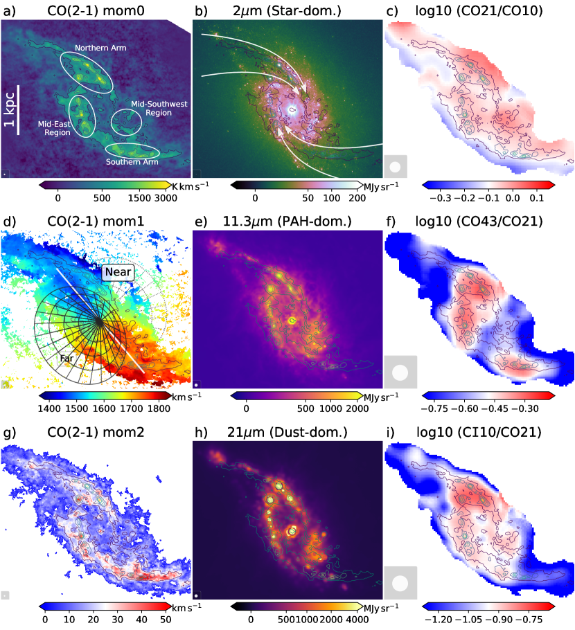
Fig. 1: ALMA and JWST images of NGC 1365. Left column (a, d, g): Native-resolution ($0.3^{\prime\prime}$) ALMA CO(2-1) integrated intensity (mom0), line-of-sight velocity (mom1) and velocity dispersion (mom2); see also Schinnerer et al. (subm.). Middle column (b, e, h): JWST stellar continuum dominated NIRCam 2 $\mu\mathrm{m}$, PAH-dominated MIRI 11.3 $\mu\mathrm{m}$, and dust continuum dominated MIRI 21 $\mu\mathrm{m}$, all at native resolutions; see also Whitmore et al. (subm.). Right column (c, f, i): Ratio maps in logarithmic scale for ${R_{21}}=I_{\mathrm{CO}\,(2\textnormal{--}1)}/I_{\mathrm{CO}\,(1\textnormal{--}0)}$, ${R_{42}}=I_{\mathrm{CO}\,(4\textnormal{--}3)}/I_{\mathrm{CO}\,(2\textnormal{--}1)}$ and ${R_{\mathrm{C}\text{\sc{i}}\mathrm{CO}}}=I_{[\mathrm{C}\,{\text{\sc{i}}}]\,(1\textnormal{--}0)}/I_{\mathrm{CO}\,(2\textnormal{--}1)}$ at the common resolution of $3.5^{\prime\prime}$ (beam is shown in bottom left). Same contours of $I_{\mathrm{CO}\,(2\textnormal{--}1)}$ at 400, 1000, 1500, 2000 and 3000 $\mathrm{K\,km\,s^{-1}}$ are shown in all panels. Four regions mentioned in this work are highlighted in panel a). The cone in panel d) represents the known ionized gas outflow with a half-opening angle $50^{\circ}$, cone axis inclination $35^{\circ}$ and PA $126^{\circ}$ (Hjelm & Lindblad 1996; see also Sandqvist et al. 1995; Lindblad 1999; Venturi et al. 2018; Gao et al. 2021) and the white line indicates the disk kinematic major axis at PA $220^{\circ}$ (Jorsater & van Moorsel 1995; Lindblad 1999).

2.2 ALMA observations of CO(1–0), (2–1) and (4–3), and [C i](1–0)

We have obtained new ALMA ACA (7m) Band 8 observations (program 2019.1.01635.S, PI: D. Liu) that map the CO(4–3) and [C i](1–0) from the inner part of NGC 1365. The CO(4–3) observations at 458.53 GHz cover the inner $75^{\prime\prime}\times 22^{\prime\prime}$ ($7.3\times 2.1$ kpc²) using a 19-pointing mosaic and on-source integration time of $\sim 1$ hour and had $T_{\mathrm{sys}}\sim 550$ K. The [C i](1–0) observations at 489.48 GHz covered the same area using a 23-pointing mosaic and an on-source integration time of $\sim 8$ hours with $T_{\mathrm{sys}}\sim 500\text{--}1000$ K. The raw data were reduced using the standard ALMA calibration pipeline with CASA software (CASA Team et al., 2022).

We also reduced archival ALMA 12m+7m observations of CO(1–0) (2015.1.01135.S, PI: F. Egusa; 2017.1.00129.S, PI: K. Morokuma), 12m+7m observations of CO(2–1) (2013.1.01161.S, PI: K. Sakamoto), including the CO(1–0) and (2–1) total power (TP) data.

After running the ALMA pipeline, we imaged and processed our data into data cubes using the PHANGS–ALMA pipeline  (Leroy et al., 2021b). Then we used the spectral_cube software to convolve our cubes to the common beam of $3.5^{\prime\prime}$ matching the coarsest C i data.

The native resolution of the CO(1–0) and (2–1) data are $2.4^{\prime\prime}$ and $0.31^{\prime\prime}$. Based on the arrays used, these images have maximum recoverable scales (MRS) of $\sim 80^{\prime\prime}$ and $40^{\prime\prime}$, respectively. Our CO(4–3) and [C i](1–0) data have $3.4\text{--}3.5^{\prime\prime}$ beams and $15\text{--}20^{\prime\prime}$ MRSs. For CO(1–0) and (2–1) the short-spacing is corrected with the PHANGS–ALMA pipeline using their total power data, however, other lines lack the short-spacing correction. We considered using the archival 12m-only ALMA CO(3–2) data for this galaxy but found that its poor $u-v$ coverage made it not useful in the analysis presented.

We expect only a minor percentage of missing flux for our CO(4–3) and [C i](1–0) data (e.g., $\lesssim 25\%$). Indeed, our total CO(4–3) line luminosity within a radius $\sim 14^{\prime\prime}$ is $5.3\times 10^{8}\ \mathrm{K\,km\,s^{-1}\,pc^{2}}$, which is more than half of the total Herschel SPIRE FTS CO(4–3) luminosity within a $\sim 43^{\prime\prime}$ beam ($7.3\times 10^{9}\pm 1.2\times 10^{7}\ \mathrm{K\,km\,s^{-1}\,pc^{2}}$; Liu et al. 2015; scaled to the same distance). Simulations of visibilities mimicking similar ACA Band 8 observations also reveal that the missing flux is minimal at relatively bright line emission spots ($\lesssim 10\%$; D. Liu et al. submitted).

We collapsed the data cubes into moment maps using the PHANGS-ALMA imaging and post-processing pipeline. We specifically focus on the “strict,” high-confidence mask, which is constructed using a watershed algorithm with relatively high clipping values (Rosolowsky & Leroy 2006; Rosolowsky et al. 2021) and so expected to include only significant detections. We build a single common strict mask by combining the individual masks for CO(1–0), CO(2–1), CO(4–3) and $[\mathrm{C}\,{\text{\sc{i}}}]\,(1\textnormal{--}0)$, then we extracted moment maps for each line therein. The error maps are also measured from the data cube, then computed for moment maps following the standard procedures implemented in the PHANGS–ALMA pipeline. In our final moment-0 maps, the S/N is 5–200 for CO(4–3), 5–100 for $[\mathrm{C}\,{\text{\sc{i}}}]\,(1\textnormal{--}0)$, and much higher (20–250) for CO(1–0) and CO(2–1). We create line ratio maps from every pair or lines at the best common resolution of $3.5^{\prime\prime}$ and use them to compute correlations and CO SLEDs.

2.3 Auxiliary data products and complementary information

We use the YMC catalog from Whitmore et al. (subm., this Issue) to determine the locations where CO and C i line fluxes are extracted and studied. It contains 37 YMCs with HST or JWST photometry derived masses $M_{\star}\sim 1\times 10^{6}\ \text{--}\ 2\times 10^{7}\ \mathrm{M_{\odot}}$ and ages $\sim 1\ \text{--}\ 8\ \mathrm{Myr}$.

We use the CO(2–1) line-of-sight decomposition and orbital time information from Schinnerer et al. (subm., this Issue) for discussions relating to line velocity dispersion. Schinnerer et al. (subm.) present the $0.3^{\prime\prime}$-resolution CO(2–1) data and decomposition of each line-of-sight spectrum into multiple Gaussian components with the ScousePy software (Henshaw et al., 2016, 2019). They find that multiple velocity components exists in the system, and individual components have a typical line width $\sigma\sim 19\ \mathrm{km\,s^{-1}}$. We use this value as the microturbulent line width $\sigma$ for our later radiative transfer calculation. They derive a dynamical timescale $t_{\mathrm{dyn}}\sim 20\ \mathrm{Myr}$ at $R=5^{\prime\prime}\approx 475\,\mathrm{pc}$, which is roughly the radius of the dynamically cold inner gas disk in this starburst ring system. This time scale is used as a context for discussion in this work.

3 Results & Discussion

3.1 Spatial and kinematic structure

In Fig. 1 we present the ALMA and JWST data at their native resolution ($\sim 6$ pc at 2 $\mu\mathrm{m}$, $\sim 30$ pc for CO(2–1) and $\sim 60$ pc at 21 $\mu\mathrm{m}$) and the multi-$J$ CO and C i ratio maps at their common resolution of $3.5^{\prime\prime}$ ($\sim 330$ pc). We define ${R_{21}}=I_{\mathrm{CO}\,(2\textnormal{--}1)}/I_{\mathrm{CO}\,(1\textnormal{--}0)}$ to trace the low-$J$ CO excitation, ${R_{42}}=I_{\mathrm{CO}\,(4\textnormal{--}3)}/I_{\mathrm{CO}\,(2\textnormal{--}1)}$ for the mid-$J$ excitation, and ${R_{\mathrm{C}\text{\sc{i}}\mathrm{CO}}}=I_{[\mathrm{C}\,{\text{\sc{i}}}]\,(1\textnormal{--}0)}/I_{\mathrm{CO}\,(2\textnormal{--}1)}$ as a tentative tracer of CO dissociation.

We also label four regions in this study to facilitate the later discussion: i) the “Northern Arm”, which is where the gas flows in from northeast along the bar; ii) the “Mid-Southwest” region, which is the downstream location of the gas coming from the Northern Arm (and we call the Northern Arm the upstream of the Mid-Southwest region); iii) the “Southern Arm”, similar to the Northern Arm, is the location of gas flowing in from the southeast along the bar; iv) the “Mid-East” region, considered as the downstream of the Southern Arm. The Northern Arm and Mid-Southwest both belong to the “northern bar lane” as defined in Schinnerer et al. (subm.), and the Southern Arm and Mid-East correspond to the “southern bar lane” therein. The Northern Arm alone is also emphasized as the “region 1” in Whitmore et al. (subm.).

The CO emission mostly arises from the prominent starburst ring, oriented from northeast to southwest, but exhibits a highly asymmetric distribution within this ring. The 2 $\mu\mathrm{m}$  stellar emission, which is much less affected by dust attenuation than HST optical images, reveals a more symmetric distribution than CO. We show the azimuthal profiles of the CO, 2 $\mu\mathrm{m}$, 11.3 $\mu\mathrm{m}$ and 21 $\mu\mathrm{m}$ emission along the starburst ring in Fig. 2. These profiles are measured from the radially-averaged emission at each azimuthal angle $\theta$ using a common annulus at our working resolution of $3.5^{\prime\prime}$. Here, $\theta=0^{\circ}$ corresponds to the receding side of major kinematic axis with PA of $220^{\circ}$, and $\theta=180^{\circ}$ ($-180^{\circ}$) to the approaching side. All azimuthal profiles show a peak at $\theta_{\mathrm{max}}\sim 150^{\circ}$, corresponding to the Northern Arm region. The 2 $\mu\mathrm{m}$ profile shows the least azimuthal variation of about 50% (with a maxima-to-minima ratio of 1.9), whereas the other three profiles show large variations $\sim 80\%\text{--}95\%$, with a maxima-to-minima ratio of 8.5, 6.0 and 19.4, for CO, 11.3 $\mu\mathrm{m}$ and 21 $\mu\mathrm{m}$  respectively.

The Northern Arm peak ($\theta\sim 150^{\circ}$) in the azimuthal profiles mainly consists of three extremely massive star clusters, YMC 29, 33 and 28, corresponding to Galliano et al. (2005, 2008) mid-IR ID M4, M5 and M6, and Sandqvist et al. (1995) radio 20 cm/6 cm ID D, E and G, respectively.

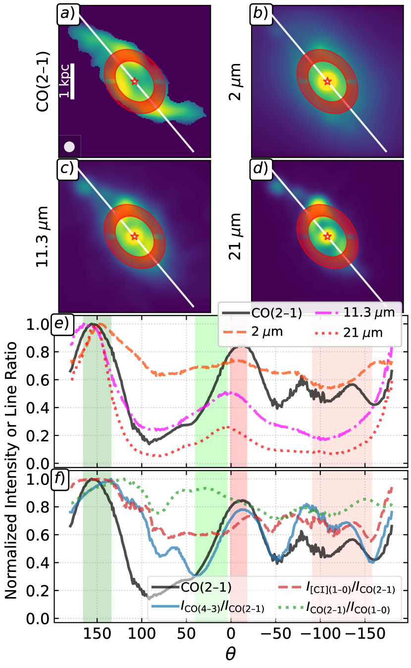
Fig. 2: Panels a)–d) are the CO(2–1) line integrated intensity, 2 $\mu\mathrm{m}$, 11.3 $\mu\mathrm{m}$ and 21 $\mu\mathrm{m}$ images, PSF-matched to our $3.5^{\prime\prime}$ resolution. A common annulus is shown in all panels with radius $=0.9\pm 0.2$ kpc, inclination $40^{\circ}$ and PA $220^{\circ}$ (white solid line Lindblad, 1999). Panels e)–f) show the normalized azimuthal profiles of the four upper panels and ${R_{42}}$, ${R_{\mathrm{C}\text{\sc{i}}\mathrm{CO}}}$ and ${R_{21}}$ line ratios as a function of azimuthal angle $\theta$ measured from the PA of the receding side of kinematic major axis. Dark green, light green, dark red and light red shading represents the Northern Arm, Mid-Southwest, Southern Arm and the Mid-East regions, respectively.

In Fig. 3 we show the distribution of YMCs on the HST RGB and JWST 2 $\mu\mathrm{m}$ image and indicate the dust lanes by two pairs of curved arrows. The CO(2–1) emission contours broadly match the dust lanes in the Northern and Southern Arm regions but appear to be narrow at the edge of dust lanes. Such dust lanes in barred galaxies are usually seen as a result of dissipative processes in the gaseous component, and the widely accepted view is that they delineate shocks in the interstellar gas (e.g., see reviews by Sellwood & Wilkinson 1993; Buta & Combes 1996; Lindblad 1999; see also Pastras et al. 2022 for detailed simulations).

In addition to the gas and dust lanes, we also highlight in Fig. 3 the YMCs younger than $\sim 3$ Myr and more attenuated than $A_{V}\sim 8$ magnitude with cyan squares and yellow stars, respectively. The majority of the most massive, young and attenuated YMCs sit in the Mid-Southwest and Mid-East regions.

The multi-$J$ CO and C i line ratio maps exhibit a significant asymmetry as well. The Northern Arm region shows a factor of 1.5–2$\times$ higher excitation and dissociation than other regions, as traced by $R_{42}$ and $R_{\mathrm{C}\text{\sc{i}}\mathrm{CO}}$. In particular, the $R_{42}$ and $R_{\mathrm{C}\text{\sc{i}}\mathrm{CO}}$ peaks coincide with the YMC ID 29 in the Northern Arm, which also corresponds to the mid-IR source M4 in Galliano et al. (2005, 2008). It has the highest CO excitation (${R_{42}}\sim 0.51\pm 0.01$, ${R_{21}}\sim 0.92\pm 0.01$) and shows the most signs of dissociation (${R_{\mathrm{C}\text{\sc{i}}\mathrm{CO}}}\sim 0.17$). The distributions of low-$J$ excitation, $R_{21}$, mid-$J$ excitation $R_{42}$, and our photodissociation tracer $R_{\mathrm{C}\text{\sc{i}}\mathrm{CO}}$ also appear distinct from one another. $R_{21}$ shows a more symmetric, smooth distribution than the other two line ratios. The $\log{R_{21}}$ is above $-0.1$ in most regions, indicating that CO(2–1) is almost thermalized in the regions we study. The $R_{42}$ and $R_{\mathrm{C}\text{\sc{i}}\mathrm{CO}}$ ratios have much larger dynamical ranges, and both peak in the Northern Arm. However, $R_{42}$ is depressed whereas $R_{\mathrm{C}\text{\sc{i}}\mathrm{CO}}$ is enhanced in the Mid-Southwest region, and their trends are the opposite in the Southern Arm region.

The molecular gas has complex, rapidly-changing kinematics in these regions. Panels (d) and (g) in Fig. 1 show the line-of-sight velocity and line velocity dispersion maps. The Northern and Southern Arm regions correspond to locations where molecular gas flows inward along the bar. The dissipative gas flow in such a strong bar potential can trigger shocks at the leading edge of the bar, appearing as dust lanes following the orbital skeleton (e.g., Athanassoula 1992; Sellwood & Wilkinson 1993; Buta & Combes 1996; Lindblad 1999; Sellwood & Masters 2022; Pastras et al. 2022; see also Fig. 1 of Maciejewski et al. 2002). In the Southern Arm, the enhanced $R_{42}$, non-enhanced $R_{\mathrm{C}\text{\sc{i}}\mathrm{CO}}$, lack of YMCs and elevated velocity dispersion $\sigma\sim 50\ \mathrm{km\,s^{-1}}$ (Fig. 1 g) may suggest a scenario where shocks triggered at the edge of dust lanes are compressing the gas and hence highly-exciting the mid-$J$ CO, but not leading to significant CO dissociation or higher C i abundance in this region. However, in other cases, e.g., the Northern Arm, when the gas is so dense and even fragments to trigger intensive star formation and hence stellar feedback, the effect of shocks can be mixed with the stellar feedback effect. Future observations of shock tracers like SiO or HNCO for less destructive shocks (e.g. Usero et al., 2006; García-Burillo et al., 2010; Meier et al., 2015; Kelly et al., 2017) will be the key to shed light on this shock scenario.

In the panel (d) of Fig. 1 we also highlight the well-known ionized gas outflow (Phillips et al., 1983; Hjelm & Lindblad, 1996; Lindblad, 1999; Sandqvist et al., 1995; Sakamoto et al., 2007; Lena et al., 2016; Venturi et al., 2018; Gao et al., 2021). We do not find a high ${R_{42}}$ nor enhanced ${R_{\mathrm{C}\text{\sc{i}}\mathrm{CO}}}$ peaking at the center and extending along the outflow cone, unlike the cases of known C i molecular outflows in AGN host galaxies (e.g., Saito et al. 2022a, b; with ${R_{\mathrm{C}\text{\sc{i}}\mathrm{CO}}}\sim 1$). This agrees with Schinnerer et al. (subm.) who find no evidence for the ionized outflow to intersect the molecular gas disk, and with Combes et al. (2019) who find that this region lacks a molecular gas outflow (and instead shows evidence for inflow).

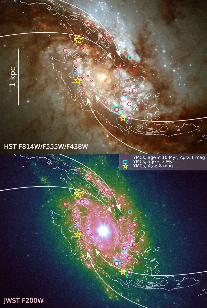
Fig. 3: YMCs (Whitmore et al., subm.) overlaid on HST RGB (F814W/F555W/F438W) image (top) and JWST F200W (2 $\mu\mathrm{m}$) image (bottom). All YMCs are shown as red circles. Symbol sizes from smallest to largest indicate masses from $\sim 10^{6.0}\;\mathrm{M}_{\odot}$ to $\sim 10^{7.1}\;\mathrm{M}_{\odot}$. Cyan squares are YMCs with an age less than $\sim 3$ Myrs, and yellow stars are YMCs with an attenuation $A_{V}>8$ magnitude. We show these YMCs for the context of the discussion in Sect. 3.1 of this work. See Whitmore et al. (subm.) for the original and detailed study of these YMCs.

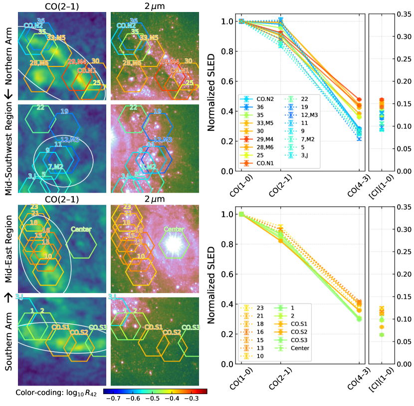
Fig. 4: Left panels: CO(2–1) and 2 ${\mu\mathrm{m}}$ zoom-in images of the Northern Arm, Mid-Southwest, Mid-East and Southern Arm regions (from top to bottom). Hexagons indicate YMCs identified by Whitmore et al. (subm.) (with numbers indicating their ID from that paper), YMC-free CO peaks (labelled “CO.N1–N2” and“CO.S1–S3” in Northern and Southern regions, respectively, visually identified from this work), and the galaxy center. The “M2”–“M6” labels indicate YMCs that have a mid-IR counterpart from Galliano et al. (2005). The “J” label indicates that YMC 3 has a radio counterpart from Sandqvist et al. (1995). All images have the same field of view of $10^{\prime\prime}$ ($\sim 950$ pc) and color scaling as in Fig. 1. Hexagons have the same diameter of $3.5^{\prime\prime}$ ($\sim 330$ pc). The black arrows at left indicate the up-to-down-stream directions. Right panels: CO and C i SLEDs of the hexagons centered at YMCs or YMC-free CO peaks in the corresponding upper/lower four left image panels. Hexagons and SLEDs are color-coded by their $R_{42}$ (see the bottom color bar). Solid and dotted lines represent up- and downstream regions, respectively. The Center’s CO SLED is shown as the dashed line in the lower panel. These CO and C i SLEDs are used for the radiative transfer modeling fitting in Sect. 3.2 with gas properties reported in Table 2.

3.2 Zoom-in views and CO and C i excitation

We examine the aforementioned regions in more detail in Fig. 4. We first draw hexagonal apertures centered on bright YMCs (Whitmore et al., subm.), CO peaks that do not coincide with a YMC (based on Fig. 4, hereafter YMC-free CO peaks, labeled as CO.N1/N2 and CO.S1/S2/S3 for those in the Northern and Southern Arms, respectively), and the galaxy center, each with a 330 pc diameter. Then, we take the pixel value at the hexagon center from the $3.5^{\prime\prime}$-resolution moment-0 map for each line, and show their normalized CO and C i SLED in the right panels of Fig. 4. The hexagons in the left panels are then color-coded by their mid-$J$ excitation ${R_{42}}$. In this way we can clearly see how gas in the apertures is excited.

The most (mid-$J$) excited aperture is YMC 29 (M4) coinciding with the brightest CO peak in the Northern Arm, with ${R_{42}}=0.50\pm 0.01$ (and ${R_{21}}=0.92\pm 0.01$, ${R_{41}}=0.46\pm 0.01$). Its stellar age is estimated as $\sim 3$ Myr (with a $\sim 0.4$–0.6 dex uncertainty; Whitmore et al. subm.). The least (mid-$J$) excited aperture we analyzed is YMC 12 (M3) in the Mid-Southwest region, with ${R_{42}}=0.24\pm 0.02$. However, its low-$J$ excitation is still quite high, with ${R_{21}}=\ 0.98\pm 0.02$. It is also very young, with a stellar age $\sim 3$ Myr (with a similarly large uncertainty; Whitmore et al. subm.). Other YMCs and YMC-free CO peaks have ${R_{42}}$ values in-between these two extreme cases.

Based on the motion of gas along the dust lanes and starburst ring (Figs. 1–3), the Northern Arm is upstream of the Mid-Southwest region, and the Southern Arm is upstream of the Mid-East region. Gas enters the system first via the Northern/Southern Arms then moves to the Mid-Southwest/Mid-East regions, forming the starburst ring. Along the Northern Arm, gas moves from the less-excited CO.N2 location to the highly-excited CO.N1 position. Then, in about a quarter of the orbital time, e.g., $\sim 5$ Myr, the gas will arrive in the Mid-Southwest region, where the CO excitation is decreasing again. It is expected that gas will move from the Mid-Southwest region towards the Southern Arm and possibly trigger collision and compression. Similarly, starting from the Southern Arm, the gas moves from CO.S3 to CO.S2 and CO.S1 positions, then circles to the Mid-East region, and heads towards the Norther Arm. The youngest YMCs are found in these possibly colliding areas, i.e., YMC 3 (J) and YMC 28 (M6, G), which both have an age $\sim 1$ Myr and are highlighted as yellow stars in Fig. 3. 

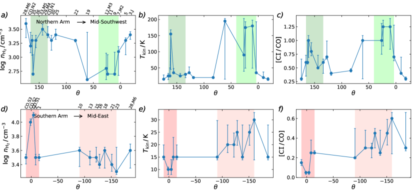
Fig. 5: Non-LTE LVG model fitting results for CO and C i SLEDs in hexagon apertures (see Fig. 4) in the Northern Arm to Mid-Southwest regions (upper panels) and Southern Arm to Mid-East regions (lower panels), respectively. The $x$-axis is the azimuthal angle starting clockwise from the PA $=220^{\circ}$ direction, same as in Fig. 2. Dark/light green and red shadings indicate the $\theta$ range of the corresponding regions. The $y$-axes show (from left to right) gas volume density ($\mathrm{log}\,n_{\mathrm{H_{2}}}$), kinetic temperature ($T_{\mathrm{kin}}$) and the $[\mathrm{C}{\text{\sc{i}}/\mathrm{CO}]}$ abundance ratio. Hexagon IDs are indicated at the top of the left panels at their corresponding $\theta$. Error bars are the $\pm 1\sigma$ uncertainty from the fitting (based on MICHI2; Liu et al. 2021; see also Appendix A). We discuss the trends of decreasing $\mathrm{log}\,n_{\mathrm{H_{2}}}$ and increasing $T_{\mathrm{kin}}$ and $[\mathrm{C}{\text{\sc{i}}/\mathrm{CO}]}$ from the upstream (dark green/red, left part of each panel) to the downstream regions (light green/red, right part of each panel) in Sect. 3.2.

To obtain a quantitative description of the gas excitation and photodissociation along the starburst ring, we perform a non-local thermodynamic (non-LTE) large velocity gradient (LVG) radiative transfer modeling of the CO and C i SLEDs for the YMC apertures and CO peaks to evaluate the gas density and temperature and $[\mathrm{C}{\text{\sc{i}}/\mathrm{CO}]}$ abundance ratio. We use the MICHI2 Monte Carlo fitting tool (Liu et al. 2021), with templates generated by the RADEX software (van der Tak et al., 2007) with a grid of gas kinetic temperature $T_{\mathrm{kin}}\sim 5\textit{--}200\ \mathrm{K}$, H₂ volume density ($\log n_{\mathrm{H_{2}}}/\mathrm{cm^{-3}}=2.0\text{--}5.0$), $[\mathrm{C}{\text{\sc{i}}/\mathrm{CO}]}$ abundance ratio 0.05–3.0, and a fixed line turbulence FWHM ${\Delta v}=45\ \mathrm{km\,s^{-1}}$ (matching the average CO line width of $\sigma\sim 19\ \mathrm{km\,s^{-1}}$ inferred at 30 pc resolution; Schinnerer et al. subm.; and Fig. 1), as well as a free beam filling factor . We show examples of our LVG fitting to the most and least excited YMC apertures, YMC 29 (M4) and YMC 12 (M3), respectively, in Appendix A. We find $\log(n_{\mathrm{H_{2}}}/\mathrm{cm^{-3}})\sim 3.50^{+0.09}_{-0.11}$ and $\sim 2.80^{+0.27}_{-0.20}$, and $T_{\mathrm{kin}}\sim 25^{+8}_{-2}$ K and $\sim 90^{+113}_{-51}$ K, respectively. Table 2 reports the best-fit parameters and 1-$\sigma$ uncertainties for all apertures.

In Fig. 5 we present the LVG fitting results for all apertures whose CO plus C i SLEDs are shown in Fig. 4. The fitted $\mathrm{log}\,n_{\mathrm{H_{2}}}$, $T_{\mathrm{kin}}$ and $[\mathrm{C}{\text{\sc{i}}/\mathrm{CO}]}$ are plotted as functions of azimuthal angle $\theta$ (see Fig. 2). In the upper panels of Fig. 5, $\theta$ ranges from $\sim 160^{\circ}$ to $\sim 10^{\circ}$, in clockwise direction tracking the gas movement from the Northern Arm (dark green shading) to the Mid-Southwest region (light green shading). Similarly, in the lower panels of Fig. 5, $\theta$ spans $\sim 0^{\circ}$ to $\sim-150^{\circ}$, in clockwise direction from the Southern Arm (dark red shading) to the Mid-East region (light red shading). We find tentative trends that $\mathrm{log}\,n_{\mathrm{H_{2}}}$ is lower, $T_{\mathrm{kin}}$ is higher and $[\mathrm{C}{\text{\sc{i}}/\mathrm{CO}]}$ is higher downstream the gas flow. The $[\mathrm{C}{\text{\sc{i}}/\mathrm{CO}]}$ ratio increases up to $\sim 1.4$ at the Mid-Southwest YMC 13, YMC 12 (M3) and YMC 10 locations. Such a high C i abundance relative to CO is likely due to the strong radiation field created by the YMCs in a relatively diffuse molecular gas.

Therefore, we propose a scenario where gas arriving from the dust lanes is piled up, compressed and shocked at the Arm regions, and YMCs are formed; then gas and YMCs travel to the downstream region during about a quarter of the orbital period (a few Myrs); the gas may continue forming stars (clusters) on the way, but must undergo strong stellar feedback, so that it is heated and C i-enriched upon its arrival in the Mid-Southwest/Mid-East regions, as our LVG fitting results suggest.

We caution that the above picture still needs higher-resolution observational supports. The trends are only significant in the Northern Arm to Mid-Southwest side ($T_{\mathrm{kin}}$ increases from below $50$ K to above $100$ K and $[\mathrm{C}{\text{\sc{i}}/\mathrm{CO}]}$ increases by a factor of two). The other side of the starburst ring from Southern Arm to Mid-East region indeed has much weaker temperature and $[\mathrm{C}{\text{\sc{i}}/\mathrm{CO}]}$ variations. The variations of $n_{\mathrm{H}_{2}}$, $T_{\mathrm{kin}}$ and $[\mathrm{C}{\text{\sc{i}}/\mathrm{CO}]}$ along the ring are also highly non-monotonous. We note that the environment in this starburst ring system is highly dynamic and stochastic. The density of the inflow cold gas feeding the starburst ring likely has an impact on how much the stellar feedback can affect the natal molecular gas. The Southern Arm gas density is much higher than that of the Northern Arm from our fitting, in line with the gas in the Southern Arm/Mid East regions being more shielded and less affected by the stellar feedback.

Finally, although the galaxy center hosts a Seyfert 1.5 AGN and a prominent [O iii] ionized gas outflow (Phillips et al. 1983; Lindblad 1999; Sandqvist et al. 1995; Hjelm & Lindblad 1996; Venturi et al. 2018; Sakamoto et al. 2007; Gao et al. 2021), it shows only moderately excited CO and C i. As shown in the next section, the center’s line ratios tracing CO excitation and dissociation are consistent with other regions when correlating these line ratios with mid-IR emission. At our resolution, we do not find any evidence of an extreme XDR such as a highly-excited CO SLED as seen in, e.g., Mrk 231 (van der Werf et al. 2010), NGC 1068 (Spinoglio et al. 2012), and other local ultra-luminous IR galaxies whose global ${R_{41}}$ are highly-excited or even close to being thermalized ($\sim 0.85\text{--}1.1$; see also Rangwala et al. 2011; Meijerink et al. 2013; Kamenetzky et al. 2014, 2016, 2017; Glenn et al. 2015; Liu et al. 2015; Rosenberg et al. 2015; Lu et al. 2017). We observe $I_{[\mathrm{C}\,{\text{\sc{i}}}]\,(1\textnormal{--}0)}/I_{\mathrm{CO}\,(1\textnormal{--}0)}=0.10$ and $I_{[\mathrm{C}\,{\text{\sc{i}}}]\,(1\textnormal{--}0)}/I_{\mathrm{CO}\,(2\textnormal{--}1)}=0.11$ in NGC 1365’s center at 330 pc-resolution. The fitted $[\mathrm{C}{\text{\sc{i}}/\mathrm{CO}]}$ is $0.25^{+0.23}_{-0.01}$ (Table 2). These line ratios and abundance ratio are much lower than those measured in the more powerful AGNs in NGC 7469 (Izumi et al., 2020) and NGC 1068 (Saito et al., 2022a, b), which have $I_{[\mathrm{C}\,{\text{\sc{i}}}]\,(1\textnormal{--}0)}/I_{\mathrm{CO}\,(1\textnormal{--}0)}\sim 0.5\text{--}1$ and $[\mathrm{C}{\text{\sc{i}}/\mathrm{CO}]}\gtrsim 1$.

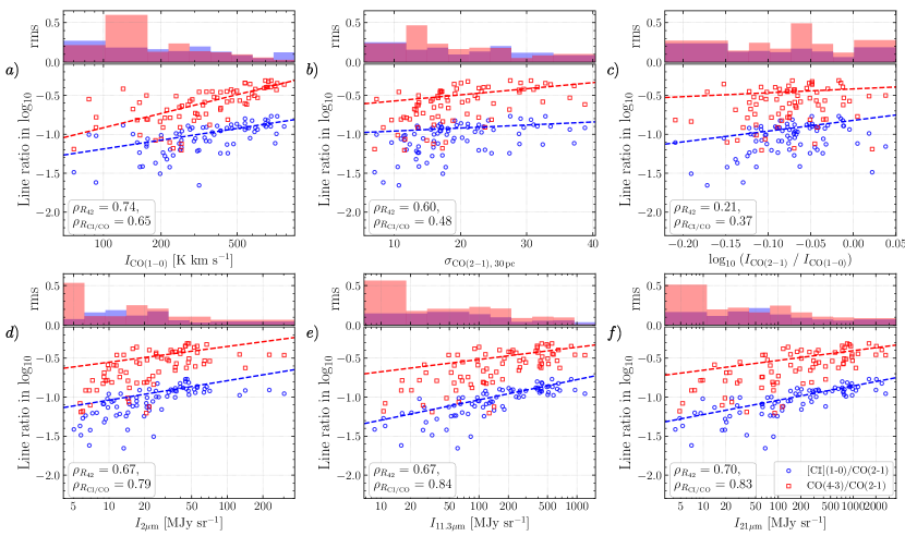
Fig. 6: Panels a) to f): $R_{42}$ in red and $R_{\mathrm{C}\text{\sc{i}}\mathrm{CO}}$ in blue as functions of six variables at 330 pc resolution across the inner part of NGC 1365: a) CO(1–0) line-integrated intensity, b) velocity dispersion, c) $R_{21}$ line ratio, d) 2 ${\mu\mathrm{m}}$, e) 11.3 ${\mu\mathrm{m}}$, and f) 21 ${\mu\mathrm{m}}$ emission. Dashed lines are the best-fit trends and legends show the Spearman rank correlation coefficients, which are also reported in Table 1. Each inset upper panel shows the rms distribution of the data after subtracting the best-fit trend in bins of the horizontal-axis variable.

	$\log_{10}I_{[\mathrm{C}\tt{I}](1\text{--}0)}/I_{\mathrm{CO}(2\text{--}1)}$					$\log_{10}I_{\mathrm{CO}(4\text{--}3)}/I_{\mathrm{CO}(2\text{--}1)}$
$x$ variable	$N$	$A$	$\rho$	$P_{0}$	rms	$N$	$A$	$\rho$	$P_{0}$	rms
1) $\log_{10}I_{\mathrm{CO}(1\text{--}0)}$	$0.38$	$-1.94$	$0.65$	$<0.001$	$0.16$	$0.61$	$-2.13$	$0.74$	$<0.001$	$0.25$
2) $\sigma_{\mathrm{CO}(2\text{--}1),\;30\,\mathrm{pc}}$	$0.00$	$-1.00$	$0.48$	$<0.001$	$0.19$	$0.01$	$-0.65$	$0.60$	$<0.001$	$0.28$
3) $\log_{10}(I_{\mathrm{CO}(2\text{--}1)}/I_{\mathrm{CO}(1\text{--}0)})$	$1.38$	$-0.82$	$0.37$	$0.001$	$0.18$	$0.50$	$-0.42$	$0.21$	$0.064$	$0.30$
4) $\log_{10}I_{\mathrm{2\mu\mathrm{m}}}$	$0.25$	$-1.29$	$0.79$	$<0.001$	$0.15$	$0.20$	$-0.75$	$0.67$	$<0.001$	$0.27$
5) $\log_{10}I_{\mathrm{11.3\mu\mathrm{m}}}$	$0.26$	$-1.56$	$0.84$	$<0.001$	$0.12$	$0.16$	$-0.83$	$0.67$	$<0.001$	$0.26$
6) $\log_{10}I_{\mathrm{21\mu\mathrm{m}}}$	$0.18$	$-1.41$	$0.83$	$<0.001$	$0.13$	$0.13$	$-0.78$	$0.70$	$<0.001$	$0.25$

Table 1: Best-fit slope $N$ and intercept $A$ of the $y=N\cdot x+A$ lines shown in Fig. 6, where $y$ is one of the $\log_{10}{R_{\mathrm{C}\text{\sc{i}}\mathrm{CO}}}\equiv\log_{10}(I_{\mathrm{[C{\tt{I}}](1\text{--}0)}}/I_{\mathrm{CO(2\text{--}1)}})$ and $\log_{10}{R_{42}}\equiv\log_{10}(I_{\mathrm{CO(4\text{--}3)}}/I_{\mathrm{CO(2\text{--}1)}})$ line ratios, and $x$ is one of the variables to correlate with: 1) the CO(1–0) integrated intensity $\log_{10}I_{\mathrm{CO(1\text{--}0)}}$; 2) the high-resolution ($\sim 30$ pc) CO(2–1) moment-2 map, convolved to the $3.5^{\prime\prime}$ ($\sim 330$ pc) resolution $\sigma_{\mathrm{CO(2\text{--}1)},\;30\,\mathrm{pc}}$; 3) the low-$J$ CO line ratio $\log_{10}(I_{\mathrm{CO(2\text{--}1)}}/I_{\mathrm{CO(1\text{--}0)}})$; 4) the stellar continuum dominated 2 $\mu\mathrm{m}$ emission $\log_{10}I_{\mathrm{2\mu\mathrm{m}}}$; 5) the PAH dominated 11.3 $\mu\mathrm{m}$ emission $\log_{10}I_{\mathrm{11.3\mu\mathrm{m}}}$; and 6) the dust continuum dominated 21 $\mu\mathrm{m}$ emission $\log_{10}I_{\mathrm{21\mu\mathrm{m}}}$. For each of ${R_{\mathrm{C}\text{\sc{i}}\mathrm{CO}}}$ and ${R_{42}}$, we list five fitting result parameters: the best-fit slope $N$, the intercept $A$, the Spearman correlation coefficient $\rho$, the null hypothesis probability $P_{0}$, and the rms scatter of data points after subtracting the best-fit line. See Sect. 3.3 for details.

3.3 Correlations of CO and C i line ratios

We investigate what star formation and ISM properties correlate with the CO and C i line ratios in Fig. 6. We examine CO(1–0) line-integrated intensity ($I_{\mathrm{CO}\,(1\textnormal{--}0)}$), molecular gas velocity dispersion ($\sigma_{\mathrm{CO(2\text{--}1),\,30~{}pc}}$ ), $R_{21}$, 21 ${\mu\mathrm{m}}$, PAH-dominated 11.3 ${\mu\mathrm{m}}$, and stellar continuum dominated 2 ${\mu\mathrm{m}}$ intensities, all at PSF-matched $3.5^{\prime\prime}$ ($\sim 330$ pc) resolution and sampled in independent resolution units (by binning in hexagons with diameter equaling the beam FWHM $3.5^{\prime\prime}$ then taking the aperture center value). For each pair of variables, we perform a linear fitting in log-log space with the scipy.optimize.curve_fit code, including errors on the line ratio propagated the original moment and uncertainty maps (Sect. 2.2). We obtain a best-fit slope $N$ and intercept $A$ for each fit and calculate the rms of the data points around the best-fitting line. We also calculate the Spearman correlation coefficient, $\rho$, and null hypothesis probability, $P_{0}$, using the pingouin code. The resulting parameters are summarized in Table 1.

The properties that correlate the most strongly with $R_{42}$ and $R_{\mathrm{C}\text{\sc{i}}\mathrm{CO}}$ are the PAH-dominated 11.3 ${\mu\mathrm{m}}$, the dust continuum dominated 21 ${\mu\mathrm{m}}$ and the stellar dominated 2 ${\mu\mathrm{m}}$ emission, with $\rho>0.7$. The $I_{\mathrm{CO}\,(1\textnormal{--}0)}$ is the next strongly correlated variable. The velocity dispersion, $\sigma_{\mathrm{CO(2\text{--}1),\,30~{}pc}}$, and ${R_{21}}$ show weak or no correlation, with $\rho\lesssim 0.3$.

For each scatter plot panel in Fig. 6, we show the rms distribution of the data in bins of the horizontal-axis variable. In all cases (except for ${R_{21}}$, panel $c$) the rms is higher at lower $x$-axis values. For all variables except $I_{\mathrm{CO}\,(1\textnormal{--}0)}$ (panel $a$), $R_{42}$ and $R_{\mathrm{C}\text{\sc{i}}\mathrm{CO}}$ tend to lie below the fitted line at the faint end. In regions with low CO intensities, the CO(4–3) line can still be as highly excited as CO-brightest regions, despite a factor of $\sim 10$ weaker CO(1–0) emission. This may be surprising if the CO(1–0) emission indeed indicates lower gas surface density and perhaps volume density, but these regions might also simply show low CO(1–0) at 330 pc resolution because of a low area filling fraction. Obtaining higher-resolution high-$J$ CO and C i observations is critical to understanding the scenarios in the future.

In panel $b)$ of Fig. 6, we find no correlations of ${R_{42}}$ or ${R_{\mathrm{C}\text{\sc{i}}\mathrm{CO}}}$ versus $\sigma_{\mathrm{CO}}$, with slope $\sim 0$. This indicates that CO excitation and C i enrichment correlate more strongly with radiation properties than with gas dynamics in this starburst ring. Indeed, in Fig. 1 (g), we find a peak $\sigma_{\mathrm{CO}}\sim 50\;\mathrm{km\,s^{-1}}$ at the Southern Arm, whereas the Northern Arm with the strongest star formation and most numerous YMCs has nearly half that value, i.e., $\sigma_{\mathrm{CO}}\sim 20\text{--}30\;\mathrm{km\,s^{-1}}$. Schinnerer et al. (subm.) find that the CO emission in this system is usually composed of multiple (e.g. 2–4) line-of-sight velocity components, with individual component having a similar line width $\sigma\sim 19\;\mathrm{km\,s^{-1}}$. Therefore, this geometry effect may well blend out any $\sigma_{\mathrm{CO}}$ versus line ratios trends in this study.

In panel $c)$ of Fig. 6, the poor correlation between $R_{21}$ and $R_{42}$ at our $\sim 330$ pc resolution indicates that the low-$J$ and mid-$J$ CO SLED shapes are largely decoupled. ${R_{21}}$ is mostly saturated/thermalized in environments like the center of NGC 1365. It is therefore necessary to obtain higher-$J$ CO lines to trace the CO excitation.

The stellar dominated 2 $\mu\mathrm{m}$, PAH-dominated 11.3 $\mu\mathrm{m}$, and warm dust continuum dominated 21 $\mu\mathrm{m}$ emission all show tight, positive correlations with the line ratios as seen in panels $d)$ to $f)$ of Fig. 6. These correlations are robust (i.e., tighter than about 0.2 dex) in the range of $10\lesssim I_{2\,{\mu\mathrm{m}}}/[\mathrm{MJy\,sr^{-1}}]\lesssim 80$, $20\lesssim I_{11.3\,{\mu\mathrm{m}}}/[\mathrm{MJy\,sr^{-1}}]\lesssim 1000$, and $20\lesssim I_{21\,{\mu\mathrm{m}}}/[\mathrm{MJy\,sr^{-1}}]\lesssim 2000$, respectively. The 2 $\mu\mathrm{m}$ correlation has the smallest valid range, only less than a decade, whereas the dust correlations are valid over nearly two decades. The galaxy center and its surrounding apertures are outliers in the line ratio versus $I_{2\,{\mu\mathrm{m}}}$ plot even at our $\sim 330$ pc resolution, but not for the line ratios versus PAH or dust continuum. We caution that the statistics is based on only one starburst ring system at a coarse resolution. Larger-sample studies will be critical to deeper understanding of the statistics.

Comparing the trends in $R_{42}$ to those in $R_{\mathrm{C}\text{\sc{i}}\mathrm{CO}}$, we find similar correlations relating each line ratio to the other variables. The trends with $R_{\mathrm{C}\text{\sc{i}}\mathrm{CO}}$ do tend to be tighter, with scatter about $\sim 0.05$–0.1 dex smaller than we find for $R_{42}$. This likely relates to the fact that $[\mathrm{C}\,{\text{\sc{i}}}]\,(1\textnormal{--}0)$ has a $>30\times$ lower critical density and $2\times$ lower upper level energy temperature ($E_{u}$) than CO(4–3) (e.g., Crocker et al., 2019, Table 3). This makes $[\mathrm{C}\,{\text{\sc{i}}}]\,(1\textnormal{--}0)$ more sensitive to the temperature and low-density part of the medium, which is substantially affected by the stellar feedback from embedded star formation traced by the YMCs, PAH emission, and warm dust continuum.

4 Summary

In this Letter we use multi-$J$ CO and C i line ratios to trace the CO excitation and dissociation and infer molecular gas temperature, density and feedback under the impact of YMCs in the bar-fed starbursting ring of NGC 1365. The mid-$J$ CO SLED up to CO(4–3), and the $[\mathrm{C}\,{\text{\sc{i}}}]\,(1\textnormal{--}0)$ line, together with the distribution of young ($<10\ \mathrm{Myr}$), massive ($M_{\star}\gtrsim 10^{6}\ \mathrm{M_{\odot}}$) star clusters revealed by JWST allow us to infer how the molecular gas properties are impacted by stellar feedback from YMCs as the gas enters and circulates in the starburst ring. We summarize our findings below.

• The Northern and Southern Arms have a high molecular gas density, relatively low temperature and $[\mathrm{C}{\text{\sc{i}}/\mathrm{CO}]}$ abundance ratio, with observed line ratios ${R_{21}}\sim 0.8\text{--}1$, ${R_{42}}\sim 0.45\text{--}0.51$ and ${R_{\mathrm{C}\text{\sc{i}}\mathrm{CO}}}\sim 0.1\text{--}0.2$. These are in line with the scenario where the Northern and Southern Arm regions are the locations where molecular gas flows into the starburst ring along the bar and dust lanes. Bar-induced shocks may play a key role in affecting the gas there, but further observational support is needed.

• The molecular gas in the Mid-Southwest region seems largely impacted by the stellar feedback (i.e., low ${R_{42}}$ but high ${R_{21}}$ and ${R_{\mathrm{C}\text{\sc{i}}\mathrm{CO}}}$), exhibiting a low gas density ($\log(n_{\mathrm{H}_{2}}/\mathrm{cm^{-3}})\sim 2.9$), high temperature ($\sim 100$ K) and enhanced $[\mathrm{C}{\text{\sc{i}}/\mathrm{CO}]}$ abundance ratio ($\gtrsim 1$) compared to the upstream Northern Arm ($\log(n_{\mathrm{H}_{2}}/\mathrm{cm^{-3}})\sim 3.4$, $T_{\mathrm{kin}}\sim 40$ K and $[\mathrm{C}{\text{\sc{i}}/\mathrm{CO}]}\sim 0.7$) as inferred from our LVG fitting.

• The molecular gas in the Mid-East region exhibits both a high ${R_{42}}$ and ${R_{\mathrm{C}\text{\sc{i}}\mathrm{CO}}}$, possibly due to its much higher density than that of the Mid-Southwest region and thus less impacted by the stellar feedback. Our LVG fitting infer that there is only a moderate decrease in gas density ($\log(n_{\mathrm{H}_{2}}/\mathrm{cm^{-3}})\sim 3.4$) or weak increase in temperature ($\sim 25$ K) and $[\mathrm{C}{\text{\sc{i}}/\mathrm{CO}]}$ ($\sim 0.5$) compared to the upstream Southern Arm region ($\log(n_{\mathrm{H}_{2}}/\mathrm{cm^{-3}})\sim 4.0$, $T_{\mathrm{kin}}\sim 15$ K and $[\mathrm{C}{\text{\sc{i}}/\mathrm{CO}]}\sim 0.2$).

• Through a correlation analysis, we find that the mid-$J$ CO excitation ${R_{42}}$ or the CO dissociation tracer ${R_{\mathrm{C}\text{\sc{i}}\mathrm{CO}}}$ does not obviously correlate with the low-$J$ CO excitation ${R_{21}}$, likely because the ${R_{21}}$ shows high ratios and appears nearly thermalized across the whole region. We also find little correlation between the line ratios and the apparent CO line velocity dispersion, implying that the complex gas dynamics does not affect the CO excitation and photodissociation in the starburst ring.

• We find tightest correlations between ${R_{42}}$ or ${R_{\mathrm{C}\text{\sc{i}}\mathrm{CO}}}$ and the mid-IR PAH-dominated 11.3 $\mu\mathrm{m}$ and dust continuum dominated 21 $\mu\mathrm{m}$ emission ($\rho\sim 0.67$–0.84, $\mathrm{rms}\sim 0.12$–0.27 dex). The stellar continuum dominated 2 $\mu\mathrm{m}$ emission correlates with ${R_{42}}$ and ${R_{\mathrm{C}\text{\sc{i}}\mathrm{CO}}}$ well too ($\rho\sim 0.67$–0.79, $\mathrm{rms}\sim 0.15$–0.27 dex) but the very center does not follow the trend.

• The ${R_{\mathrm{C}\text{\sc{i}}\mathrm{CO}}}$ correlations with mid-IR dust/PAH and near-IR stellar emission properties are in general slightly tighter ($\sim 0.1$ higher in $\rho$) and less scattered ($\sim-0.5$ dex smaller rms) than those of ${R_{42}}$. This may relate to the significantly lower critical density of $[\mathrm{C}\,{\text{\sc{i}}}]\,(1\textnormal{--}0)$ than $\mathrm{CO}\,(4\textnormal{--}3)$ and to CO dissociation which make C i more sensitive to the mid-IR traced bulk of star-forming gas and stellar feedback.

• Despite hosting an Seyfert 1.5 AGN and having an ionized gas outflow, NGC 1365’s central $\sim 330$ pc area (our resolution unit) exhibits only moderate CO excitation and C i/CO line ratio comparable to or even less highly excited than other regions that we studied.

Appendix A LVG model fitting

We illustrate our Monte Carlo LVG model fitting in Fig. A.1. We first use RADEX (van der Tak et al., 2007) with the Leiden Atomic and Molecular Database (Schöier et al., 2005) to build a library of LVG models with the parameter grids as described in Sect. 3.2. Then, we use the MICHI2 code (Liu et al., 2021) to run Monte Carlo fitting and obtain the $1/\chi^{2}$ posterior distribution for each parameter (following the statistical criterion of $\pm 1\sigma$ in Press et al. 1992). Blue squares with error bars are the CO and C i line fluxes to be fitted, and black to gray dots are model data points with different reduced $\chi^{2}$. Our free model parameters are $\mathrm{log}\,n_{\mathrm{H_{2}}}$, $T_{\mathrm{kin}}$, $[\mathrm{C}{\text{\sc{i}}/\mathrm{CO}]}$, and normalization (beam filling factor). Their $1/\chi^{2}$ distributions and the $\pm 1\sigma$ ranges are shown in the lower panels. All fitting results are presented in Table 2.

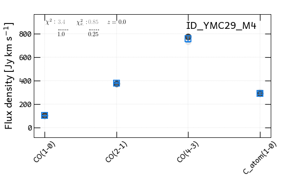
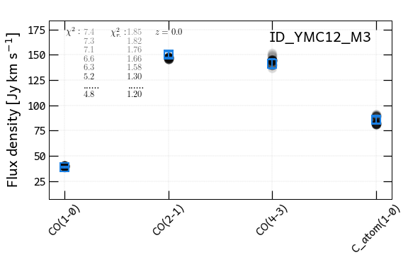
Fig. A.1: Upper row: the CO and C i SLED of YMC 29 (M4, the most excited YMC aperture in the Northern Arm; left panel) and that of YMC 12 (M3, the least excited YMC aperture in the Mid-Southwest region; right panel). Observed line fluxes are shown as blue squares with error bars. Black to gray solid circles are fitted points from a series of fitting within $1\sigma$ with an increasing $\chi^{2}$ (and reduced $\chi^{2}$, $\chi_{r}^{2}$). Bottom panels: corresponding $1/\chi^{2}$ distributions of model fitting parameters $T_{\mathrm{kin}}$, $\mathrm{log}\,n_{\mathrm{H_{2}}}$, $\log N_{\mathrm{H_{2}}}$ (non-independent) and $[\mathrm{C}{\text{\sc{i}}/\mathrm{CO}]}$ from the MICHI2 code. Yellow shading indicates the $\pm 1\sigma$ parameter range.

Aperture	RA (J2000)	DEC (J2000)	$\log n_{\mathrm{H_{2}}}/\mathrm{cm^{-3}}$	$\log N_{\mathrm{H_{2}}}/\mathrm{cm^{-2}}$	$T_{\mathrm{kin}}/\mathrm{K}$	$[\mathrm{C}\text{\sc{i}}/\mathrm{CO}]$
Northern Arm
CO.N2	$53.40340917$	$-36.13729972$	$3.20_{-0.12}^{+0.25}$	$22.44_{-0.12}^{+0.26}$	$25.0_{-11.2}^{+8.0}$	$0.60_{-0.25}^{+0.13}$
36	$53.40311543$	$-36.13715197$	$2.70_{-0.02}^{+0.35}$	$21.94_{-0.01}^{+0.36}$	$155.0_{-110.0}^{+12.9}$	$1.00_{-0.31}^{+0.09}$
35	$53.40306629$	$-36.13749402$	$3.30_{-0.26}^{+0.09}$	$22.54_{-0.25}^{+0.06}$	$25.0_{-2.3}^{+24.7}$	$0.60_{-0.03}^{+0.40}$
33,M5	$53.40251420$	$-36.13768031$	$3.30_{-0.13}^{+0.09}$	$22.54_{-0.16}^{+0.06}$	$35.0_{-3.4}^{+13.0}$	$0.80_{-0.08}^{+0.16}$
30	$53.40098220$	$-36.13841668$	$3.30_{-0.17}^{+0.09}$	$22.54_{-0.16}^{+0.06}$	$35.0_{-3.4}^{+18.0}$	$0.70_{-0.04}^{+0.29}$
29,M4	$53.40170236$	$-36.13843398$	$3.50_{-0.11}^{+0.09}$	$22.74_{-0.16}^{+0.07}$	$25.0_{-2.3}^{+8.0}$	$0.50_{-0.02}^{+0.23}$
28,M6	$53.40318107$	$-36.13847524$	$3.60_{-0.25}^{+0.09}$	$22.84_{-0.20}^{+0.07}$	$15.0_{-1.2}^{+12.9}$	$0.30_{-0.03}^{+0.36}$
25	$53.40092801$	$-36.13910029$	$3.40_{-0.08}^{+0.10}$	$22.64_{-0.09}^{+0.04}$	$20.0_{-3.1}^{+2.9}$	$0.40_{-0.04}^{+0.02}$
CO.N1	$53.40132208$	$-36.13871556$	$3.40_{-0.05}^{+0.14}$	$22.64_{-0.06}^{+0.17}$	$30.0_{-10.2}^{+3.0}$	$0.60_{-0.20}^{+0.06}$
Mid-Southwest Region
22	$53.40046102$	$-36.13984982$	$3.30_{-0.03}^{+0.02}$	$22.54_{-0.06}^{+0.01}$	$20.0_{-3.1}^{+2.9}$	$0.45_{-0.03}^{+0.03}$
19	$53.39952417$	$-36.14009082$	$2.60_{-0.01}^{+0.85}$	$21.84_{+0.00}^{+0.87}$	$195.0_{-180.0}^{+7.9}$	$1.00_{-0.70}^{+0.09}$
12,M3	$53.39955255$	$-36.14112108$	$2.80_{-0.20}^{+0.27}$	$22.04_{-0.20}^{+0.30}$	$90.0_{-50.6}^{+112.9}$	$1.00_{-0.25}^{+0.31}$
11	$53.39977124$	$-36.14112797$	$2.70_{-0.02}^{+0.35}$	$21.94_{-0.01}^{+0.36}$	$175.0_{-125.8}^{+17.9}$	$1.25_{-0.35}^{+0.12}$
9	$53.40018429$	$-36.14131523$	$2.70_{-0.02}^{+0.39}$	$21.94_{-0.08}^{+0.36}$	$180.0_{-130.8}^{+17.9}$	$1.25_{-0.41}^{+0.15}$
7,M2	$53.39987072$	$-36.14183303$	$3.10_{-0.42}^{+0.09}$	$22.34_{-0.41}^{+0.06}$	$35.0_{-3.4}^{+157.9}$	$0.70_{-0.07}^{+0.58}$
5	$53.40033806$	$-36.14207205$	$3.30_{-0.26}^{+0.04}$	$22.54_{-0.30}^{+0.06}$	$20.0_{-0.2}^{+17.4}$	$0.40_{-0.01}^{+0.30}$
3,J	$53.40069177$	$-36.14212741$	$3.40_{-0.08}^{+0.05}$	$22.64_{-0.09}^{+0.04}$	$15.0_{-4.0}^{+4.9}$	$0.30_{-0.03}^{+0.03}$
Mid-East Region
23	$53.40337423$	$-36.13956883$	$3.30_{-0.04}^{+0.35}$	$22.54_{-0.03}^{+0.36}$	$30.0_{-16.1}^{+3.0}$	$0.60_{-0.36}^{+0.06}$
21	$53.40333174$	$-36.13986047$	$3.40_{-0.10}^{+0.14}$	$22.64_{-0.06}^{+0.17}$	$25.0_{-5.2}^{+2.9}$	$0.45_{-0.12}^{+0.14}$
18	$53.40339461$	$-36.14021144$	$3.60_{-0.25}^{+0.05}$	$22.84_{-0.20}^{+0.07}$	$15.0_{-1.2}^{+12.9}$	$0.25_{-0.03}^{+0.23}$
16	$53.40291154$	$-36.14045529$	$3.40_{-0.05}^{+0.14}$	$22.64_{-0.06}^{+0.17}$	$25.0_{-5.2}^{+4.7}$	$0.45_{-0.15}^{+0.05}$
15	$53.40321229$	$-36.14061030$	$3.50_{-0.06}^{+0.14}$	$22.74_{-0.05}^{+0.16}$	$20.0_{-5.0}^{+4.7}$	$0.30_{-0.10}^{+0.05}$
13	$53.40293504$	$-36.14082502$	$3.50_{-0.11}^{+0.09}$	$22.74_{-0.10}^{+0.07}$	$20.0_{-3.2}^{+7.9}$	$0.30_{+0.00}^{+0.18}$
10	$53.40283403$	$-36.14127466$	$3.60_{-0.23}^{+0.05}$	$22.84_{-0.25}^{+0.07}$	$15.0_{-1.2}^{+14.7}$	$0.20_{+0.00}^{+0.30}$
Southern Arm
1	$53.40028097$	$-36.14257775$	$3.50_{-0.05}^{+0.05}$	$22.74_{-0.06}^{+0.00}$	$15.0_{-1.1}^{+4.9}$	$0.25_{-0.01}^{+0.02}$
2	$53.39989135$	$-36.14257526$	$3.50_{-0.11}^{+0.04}$	$22.74_{-0.10}^{+0.07}$	$15.0_{-1.2}^{+7.9}$	$0.25_{-0.01}^{+0.13}$
CO.S1	$53.39917000$	$-36.14308806$	$4.10_{-0.01}^{+0.04}$	$23.34_{-0.01}^{+0.06}$	$10.0_{-2.0}^{+3.9}$	$0.05_{-0.02}^{+0.01}$
CO.S2	$53.39845708$	$-36.14325417$	$4.00_{-0.05}^{+0.05}$	$23.24_{-0.04}^{+0.03}$	$10.0_{-2.0}^{+1.0}$	$0.05_{-0.02}^{+0.01}$
CO.S3	$53.39761333$	$-36.14309889$	$3.50_{-0.09}^{+0.05}$	$22.74_{-0.06}^{+0.00}$	$15.0_{-1.1}^{+4.9}$	$0.15_{-0.03}^{+0.03}$
Center
Center	$53.40154167$	$-36.14041694$	$3.50_{-0.24}^{+0.04}$	$22.74_{-0.23}^{+0.07}$	$15.0_{-1.2}^{+12.9}$	$0.25_{-0.01}^{+0.23}$

Table 2: Results of MICHI2 LVG fitting to the CO and C i SLED of YMC, CO peak and galaxy center apertures. YMC IDs and R.A. and Declination coordinates are from Whitmore et al. (subm.). See description of the fitting in Sect. 3.2. See also Fig. 5 for the illustration of the fitted parameters along the starburst ring.

References

- Anand et al. (2021a) Anand, G. S., Rizzi, L., Tully, R. B., et al. 2021a, AJ, 162, 80, doi: 10.3847/1538-3881/ac0440
- Anand et al. (2021b) Anand, G. S., Lee, J. C., Van Dyk, S. D., et al. 2021b, MNRAS, 501, 3621, doi: 10.1093/mnras/staa3668
- Astropy Collaboration et al. (2013) Astropy Collaboration, Robitaille, T. P., Tollerud, E. J., et al. 2013, A&A, 558, A33, doi: 10.1051/0004-6361/201322068
- Astropy Collaboration et al. (2018) Astropy Collaboration, Price-Whelan, A. M., Sipőcz, B. M., et al. 2018, AJ, 156, 123, doi: 10.3847/1538-3881/aabc4f
- Astropy Collaboration et al. (2022) Astropy Collaboration, Price-Whelan, A. M., Lim, P. L., et al. 2022, apj, 935, 167, doi: 10.3847/1538-4357/ac7c74
- Athanassoula (1992) Athanassoula, E. 1992, MNRAS, 259, 345, doi: 10.1093/mnras/259.2.345
- Audibert et al. (2019) Audibert, A., Combes, F., García-Burillo, S., et al. 2019, A&A, 632, A33, doi: 10.1051/0004-6361/201935845
- Barnes et al. (2021) Barnes, A. T., Glover, S. C. O., Kreckel, K., et al. 2021, MNRAS, 508, 5362, doi: 10.1093/mnras/stab2958
- Barnes et al. (2022) Barnes, A. T., Chandar, R., Kreckel, K., et al. 2022, A&A, 662, L6, doi: 10.1051/0004-6361/202243766
- Bayet et al. (2004) Bayet, E., Gerin, M., Phillips, T. G., & Contursi, A. 2004, A&A, 427, 45, doi: 10.1051/0004-6361:20035614
- Bayet et al. (2006) —. 2006, A&A, 460, 467, doi: 10.1051/0004-6361:20053872
- Bradley et al. (2020) Bradley, L., Sipőcz, B., Robitaille, T., et al. 2020, astropy/photutils: 1.0.0, 1.0.0, Zenodo, Zenodo, doi: 10.5281/zenodo.4044744
- Buta & Combes (1996) Buta, R., & Combes, F. 1996, Fund. Cosmic Phys., 17, 95
- Calzetti et al. (2015) Calzetti, D., Lee, J. C., Sabbi, E., et al. 2015, AJ, 149, 51, doi: 10.1088/0004-6256/149/2/51
- CASA Team et al. (2022) CASA Team, Bean, B., Bhatnagar, S., et al. 2022, PASP, 134, 114501, doi: 10.1088/1538-3873/ac9642
- Chevance et al. (2022) Chevance, M., Krumholz, M. R., McLeod, A. F., et al. 2022, arXiv e-prints, arXiv:2203.09570. https://arxiv.org/abs/2203.09570
- Chevance et al. (2020) Chevance, M., Kruijssen, J. M. D., Hygate, A. P. S., et al. 2020, MNRAS, 493, 2872, doi: 10.1093/mnras/stz3525
- Cicone et al. (2018) Cicone, C., Brusa, M., Ramos Almeida, C., et al. 2018, Nature Astronomy, 2, 176, doi: 10.1038/s41550-018-0406-3
- Combes et al. (2019) Combes, F., García-Burillo, S., Audibert, A., et al. 2019, A&A, 623, A79, doi: 10.1051/0004-6361/201834560
- Crocker et al. (2019) Crocker, A. F., Pellegrini, E., Smith, J. D. T., et al. 2019, ApJ, 887, 105, doi: 10.3847/1538-4357/ab4196
- Curran et al. (2001) Curran, S. J., Polatidis, A. G., Aalto, S., & Booth, R. S. 2001, A&A, 368, 824, doi: 10.1051/0004-6361:20010091
- de Jong et al. (1980) de Jong, T., Boland, W., & Dalgarno, A. 1980, A&A, 91, 68
- Emsellem et al. (2022) Emsellem, E., Schinnerer, E., Santoro, F., et al. 2022, A&A, 659, A191, doi: 10.1051/0004-6361/202141727
- Erroz-Ferrer et al. (2019) Erroz-Ferrer, S., Carollo, C. M., den Brok, M., et al. 2019, MNRAS, 484, 5009, doi: 10.1093/mnras/stz194
- Fazeli et al. (2019) Fazeli, N., Busch, G., Valencia-S., M., et al. 2019, A&A, 622, A128, doi: 10.1051/0004-6361/201834255
- Fukui et al. (2016) Fukui, Y., Torii, K., Ohama, A., et al. 2016, ApJ, 820, 26, doi: 10.3847/0004-637X/820/1/26
- Gadotti et al. (2019) Gadotti, D. A., Sánchez-Blázquez, P., Falcón-Barroso, J., et al. 2019, MNRAS, 482, 506, doi: 10.1093/mnras/sty2666
- Galliano et al. (2008) Galliano, E., Alloin, D., Pantin, E., et al. 2008, A&A, 492, 3, doi: 10.1051/0004-6361:20077621
- Galliano et al. (2005) Galliano, E., Alloin, D., Pantin, E., Lagage, P. O., & Marco, O. 2005, A&A, 438, 803, doi: 10.1051/0004-6361:20053049
- Gao et al. (2021) Gao, Y., Egusa, F., Liu, G., et al. 2021, ApJ, 913, 139, doi: 10.3847/1538-4357/abf738
- García-Burillo et al. (2010) García-Burillo, S., Usero, A., Fuente, A., et al. 2010, A&A, 519, A2, doi: 10.1051/0004-6361/201014539
- García-Burillo et al. (2021) García-Burillo, S., Alonso-Herrero, A., Ramos Almeida, C., et al. 2021, A&A, 652, A98, doi: 10.1051/0004-6361/202141075
- Ginsburg et al. (2019) Ginsburg, A., Koch, E., Robitaille, T., et al. 2019, radio-astro-tools/spectral-cube: v0.4.4, v0.4.4, Zenodo, Zenodo, doi: 10.5281/zenodo.2573901
- Glenn et al. (2015) Glenn, J., Rangwala, N., Maloney, P. R., & Kamenetzky, J. R. 2015, ApJ, 800, 105, doi: 10.1088/0004-637X/800/2/105
- Goldreich & Kwan (1974) Goldreich, P., & Kwan, J. 1974, ApJ, 189, 441, doi: 10.1086/152821
- Grasha et al. (2018) Grasha, K., Calzetti, D., Bittle, L., et al. 2018, MNRAS, 481, 1016, doi: 10.1093/mnras/sty2154
- Greve et al. (2014) Greve, T. R., Leonidaki, I., Xilouris, E. M., et al. 2014, ApJ, 794, 142, doi: 10.1088/0004-637X/794/2/142
- Harrison et al. (2018) Harrison, C. M., Costa, T., Tadhunter, C. N., et al. 2018, Nature Astronomy, 2, 198, doi: 10.1038/s41550-018-0403-6
- Henshaw et al. (2016) Henshaw, J. D., Longmore, S. N., Kruijssen, J. M. D., et al. 2016, MNRAS, 457, 2675, doi: 10.1093/mnras/stw121
- Henshaw et al. (2019) Henshaw, J. D., Ginsburg, A., Haworth, T. J., et al. 2019, MNRAS, 485, 2457, doi: 10.1093/mnras/stz471
- Hjelm & Lindblad (1996) Hjelm, M., & Lindblad, P. O. 1996, A&A, 305, 727
- Hollenbach et al. (1991) Hollenbach, D. J., Takahashi, T., & Tielens, A. G. G. M. 1991, ApJ, 377, 192, doi: 10.1086/170347
- Hollenbach & Tielens (1997) Hollenbach, D. J., & Tielens, A. G. G. M. 1997, ARA&A, 35, 179, doi: 10.1146/annurev.astro.35.1.179
- Hunter (2007) Hunter, J. D. 2007, Computing in Science & Engineering, 9, 90, doi: 10.1109/MCSE.2007.55
- Israel et al. (2015) Israel, F. P., Rosenberg, M. J. F., & van der Werf, P. 2015, A&A, 578, A95, doi: 10.1051/0004-6361/201425175
- Israel et al. (1995) Israel, F. P., White, G. J., & Baas, F. 1995, A&A, 302, 343
- Izumi et al. (2020) Izumi, T., Nguyen, D. D., Imanishi, M., et al. 2020, ApJ, 898, 75, doi: 10.3847/1538-4357/ab9cb1
- Jorsater & van Moorsel (1995) Jorsater, S., & van Moorsel, G. A. 1995, AJ, 110, 2037, doi: 10.1086/117668
- Kamenetzky et al. (2017) Kamenetzky, J., Rangwala, N., & Glenn, J. 2017, MNRAS, 471, 2917, doi: 10.1093/mnras/stx1595
- Kamenetzky et al. (2014) Kamenetzky, J., Rangwala, N., Glenn, J., Maloney, P. R., & Conley, A. 2014, ApJ, 795, 174, doi: 10.1088/0004-637X/795/2/174
- Kamenetzky et al. (2016) —. 2016, ApJ, 829, 93, doi: 10.3847/0004-637X/829/2/93
- Kaufman et al. (1999) Kaufman, M. J., Wolfire, M. G., Hollenbach, D. J., & Luhman, M. L. 1999, ApJ, 527, 795, doi: 10.1086/308102
- Kelly et al. (2017) Kelly, G., Viti, S., García-Burillo, S., et al. 2017, A&A, 597, A11, doi: 10.1051/0004-6361/201628946
- Kennicutt & Evans (2012) Kennicutt, R. C., & Evans, N. J. 2012, ARA&A, 50, 531, doi: 10.1146/annurev-astro-081811-125610
- Kim et al. (2022) Kim, J., Chevance, M., Kruijssen, J. M. D., et al. 2022, MNRAS, doi: 10.1093/mnras/stac2339
- Kristen et al. (1997) Kristen, H., Jorsater, S., Lindblad, P. O., & Boksenberg, A. 1997, A&A, 328, 483
- Kruijssen et al. (2019) Kruijssen, J. M. D., Schruba, A., Chevance, M., et al. 2019, Nature, 569, 519, doi: 10.1038/s41586-019-1194-3
- Langer (1976) Langer, W. 1976, ApJ, 206, 699, doi: 10.1086/154430
- Lee et al. (subm.) Lee, J., et al. subm., ApJ
- Lee et al. (2022) Lee, J. C., Whitmore, B. C., Thilker, D. A., et al. 2022, ApJS, 258, 10, doi: 10.3847/1538-4365/ac1fe5
- Lena et al. (2016) Lena, D., Robinson, A., Storchi-Bergmann, T., et al. 2016, MNRAS, 459, 4485, doi: 10.1093/mnras/stw896
- Leroy et al. (2021a) Leroy, A. K., Schinnerer, E., Hughes, A., et al. 2021a, ApJS, 257, 43, doi: 10.3847/1538-4365/ac17f3
- Leroy et al. (2021b) Leroy, A. K., Hughes, A., Liu, D., et al. 2021b, ApJS, 255, 19, doi: 10.3847/1538-4365/abec80
- Lindblad (1999) Lindblad, P. O. 1999, A&A Rev., 9, 221, doi: 10.1007/s001590050018
- Liu (2020) Liu, D. 2020, michi2: SED and SLED fitting tool, Astrophysics Source Code Library, record ascl:2005.002. http://ascl.net/2005.002
- Liu et al. (2015) Liu, D., Gao, Y., Isaak, K., et al. 2015, ApJ, 810, L14, doi: 10.1088/2041-8205/810/2/L14
- Liu et al. (2021) Liu, D., Daddi, E., Schinnerer, E., et al. 2021, ApJ, 909, 56, doi: 10.3847/1538-4357/abd801
- Lu et al. (2017) Lu, N., Zhao, Y., Díaz-Santos, T., et al. 2017, ApJS, 230, 1, doi: 10.3847/1538-4365/aa6476
- Maciejewski et al. (2002) Maciejewski, W., Teuben, P. J., Sparke, L. S., & Stone, J. M. 2002, MNRAS, 329, 502, doi: 10.1046/j.1365-8711.2002.04957.x
- Maloney et al. (1996) Maloney, P. R., Hollenbach, D. J., & Tielens, A. G. G. M. 1996, ApJ, 466, 561, doi: 10.1086/177532
- Meier et al. (2015) Meier, D. S., Walter, F., Bolatto, A. D., et al. 2015, ApJ, 801, 63, doi: 10.1088/0004-637X/801/1/63
- Meijerink & Spaans (2005) Meijerink, R., & Spaans, M. 2005, A&A, 436, 397, doi: 10.1051/0004-6361:20042398
- Meijerink et al. (2007) Meijerink, R., Spaans, M., & Israel, F. P. 2007, A&A, 461, 793, doi: 10.1051/0004-6361:20066130
- Meijerink et al. (2013) Meijerink, R., Kristensen, L. E., Weiß, A., et al. 2013, ApJ, 762, L16, doi: 10.1088/2041-8205/762/2/L16
- Morganti et al. (1999) Morganti, R., Tsvetanov, Z. I., Gallimore, J., & Allen, M. G. 1999, A&AS, 137, 457, doi: 10.1051/aas:1999258
- Pan et al. (2022) Pan, H.-A., Schinnerer, E., Hughes, A., et al. 2022, ApJ, 927, 9, doi: 10.3847/1538-4357/ac474f
- Papadopoulos (2010) Papadopoulos, P. P. 2010, ApJ, 720, 226, doi: 10.1088/0004-637X/720/1/226
- Papadopoulos et al. (2018) Papadopoulos, P. P., Bisbas, T. G., & Zhang, Z.-Y. 2018, MNRAS, 478, 1716, doi: 10.1093/mnras/sty1077
- Papadopoulos et al. (2007) Papadopoulos, P. P., Isaak, K. G., & van der Werf, P. P. 2007, ApJ, 668, 815, doi: 10.1086/520671
- Papadopoulos et al. (2011) Papadopoulos, P. P., Thi, W.-F., Miniati, F., & Viti, S. 2011, MNRAS, 414, 1705, doi: 10.1111/j.1365-2966.2011.18504.x
- Papadopoulos et al. (2010) Papadopoulos, P. P., van der Werf, P., Isaak, K., & Xilouris, E. M. 2010, ApJ, 715, 775, doi: 10.1088/0004-637X/715/2/775
- Pastras et al. (2022) Pastras, S., Patsis, P. A., & Athanassoula, E. 2022, Universe, 8, 290, doi: 10.3390/universe8050290
- Phillips et al. (1983) Phillips, M. M., Turtle, A. J., Edmunds, M. G., & Pagel, B. E. J. 1983, MNRAS, 203, 759, doi: 10.1093/mnras/203.3.759
- Press et al. (1992) Press, W. H., Teukolsky, S. A., Vetterling, W. T., & Flannery, B. P. 1992, Numerical recipes in C. The art of scientific computing (2nd edition) (Cambridge University Press)
- Rangwala et al. (2011) Rangwala, N., Maloney, P. R., Glenn, J., et al. 2011, ApJ, 743, 94, doi: 10.1088/0004-637X/743/1/94
- Rosenberg et al. (2015) Rosenberg, M. J. F., van der Werf, P. P., Aalto, S., et al. 2015, ApJ, 801, 72, doi: 10.1088/0004-637X/801/2/72
- Rosolowsky & Leroy (2006) Rosolowsky, E., & Leroy, A. 2006, PASP, 118, 590, doi: 10.1086/502982
- Rosolowsky et al. (2021) Rosolowsky, E., Hughes, A., Leroy, A. K., et al. 2021, MNRAS, 502, 1218, doi: 10.1093/mnras/stab085
- Saito et al. (2022a) Saito, T., Takano, S., Harada, N., et al. 2022a, ApJ, 927, L32, doi: 10.3847/2041-8213/ac59ae
- Saito et al. (2022b) —. 2022b, ApJ, 935, 155, doi: 10.3847/1538-4357/ac80ff
- Sakamoto et al. (2007) Sakamoto, K., Ho, P. T. P., Mao, R.-Q., Matsushita, S., & Peck, A. B. 2007, ApJ, 654, 782, doi: 10.1086/509775
- Salak et al. (2019) Salak, D., Nakai, N., Seta, M., & Miyamoto, Y. 2019, ApJ, 887, 143, doi: 10.3847/1538-4357/ab55dc
- Sandqvist et al. (1995) Sandqvist, A., Joersaeter, S., & Lindblad, P. O. 1995, A&A, 295, 585
- Schinnerer et al. (subm.) Schinnerer, E., et al. subm., ApJ
- Schöier et al. (2005) Schöier, F. L., van der Tak, F. F. S., van Dishoeck, E. F., & Black, J. H. 2005, A&A, 432, 369, doi: 10.1051/0004-6361:20041729
- Scoville (2013) Scoville, N. Z. 2013, in Secular Evolution of Galaxies, ed. J. Falcón-Barroso & J. H. Knapen (Cambridge University Press), 491
- Sellwood & Masters (2022) Sellwood, J. A., & Masters, K. L. 2022, ARA&A, 60, doi: 10.1146/annurev-astro-052920-104505
- Sellwood & Wilkinson (1993) Sellwood, J. A., & Wilkinson, A. 1993, Reports on Progress in Physics, 56, 173, doi: 10.1088/0034-4885/56/2/001
- Shirley (2015) Shirley, Y. L. 2015, PASP, 127, 299, doi: 10.1086/680342
- Spinoglio et al. (2012) Spinoglio, L., Pereira-Santaella, M., Busquet, G., et al. 2012, ApJ, 758, 108, doi: 10.1088/0004-637X/758/2/108
- Sun et al. (2020) Sun, J., Leroy, A. K., Schinnerer, E., et al. 2020, ApJ, 901, L8, doi: 10.3847/2041-8213/abb3be
- Tacconi et al. (2020) Tacconi, L. J., Genzel, R., & Sternberg, A. 2020, ARA&A, 58, 157, doi: 10.1146/annurev-astro-082812-141034
- Tielens & Hollenbach (1985a) Tielens, A. G. G. M., & Hollenbach, D. 1985a, ApJ, 291, 722, doi: 10.1086/163111
- Tielens & Hollenbach (1985b) —. 1985b, ApJ, 291, 747, doi: 10.1086/163112
- Turner et al. (1993) Turner, T. J., Urry, C. M., & Mushotzky, R. F. 1993, ApJ, 418, 653, doi: 10.1086/173425
- Usero et al. (2006) Usero, A., García-Burillo, S., Martín-Pintado, J., Fuente, A., & Neri, R. 2006, A&A, 448, 457, doi: 10.1051/0004-6361:20054033
- van der Tak et al. (2007) van der Tak, F. F. S., Black, J. H., Schöier, F. L., Jansen, D. J., & van Dishoeck, E. F. 2007, A&A, 468, 627, doi: 10.1051/0004-6361:20066820
- van der Werf et al. (2010) van der Werf, P. P., Isaak, K. G., Meijerink, R., et al. 2010, A&A, 518, L42, doi: 10.1051/0004-6361/201014682
- Venturi et al. (2018) Venturi, G., Nardini, E., Marconi, A., et al. 2018, A&A, 619, A74, doi: 10.1051/0004-6361/201833668
- Veron et al. (1980) Veron, P., Lindblad, P. O., Zuiderwijk, E. J., Veron, M. P., & Adam, G. 1980, A&A, 87, 245
- Virtanen et al. (2020) Virtanen, P., Gommers, R., Oliphant, T. E., et al. 2020, Nature Methods, 17, 261, doi: 10.1038/s41592-019-0686-2
- Weiß et al. (2007) Weiß, A., Downes, D., Neri, R., et al. 2007, A&A, 467, 955, doi: 10.1051/0004-6361:20066117
- Whitmore et al. (subm.) Whitmore, B., et al. subm., ApJ
- Wolfire et al. (2022) Wolfire, M. G., Vallini, L., & Chevance, M. 2022, ARA&A, 60, 247, doi: 10.1146/annurev-astro-052920-010254
- Zhang et al. (2014) Zhang, Z.-Y., Henkel, C., Gao, Y., et al. 2014, A&A, 568, A122, doi: 10.1051/0004-6361/201322639