Three-family supersymmetric Pati-Salam models with symplectic groups from intersecting D6-branes

Adeel Mansha Email: adeelmansha@zjnu.edu.cn Affiliation: Department of Physics, Zhejiang Normal University, Jinhua 321004, P. R. China Affiliation: Zhejiang Institute of Photoelectronics, Zhejiang Normal University, Jinhua 321004, P. R. China Affiliation: Zhejiang Institute for Advanced Light Source, Zhejiang Normal University, Jinhua 321004, P. R. China    Tianjun Li Email: tli@itp.ac.cn Affiliation: CAS Key Laboratory of Theoretical Physics, Institute of Theoretical Physics, Chinese Academy of Sciences, Beijing 100190, P. R. China Affiliation: School of Physical Sciences, University of Chinese Academy of Sciences, Beijing, P. R. China    Mudassar Sabir Thanks: Corresponding author Email: mudassar.sabir@uestc.edu.cn Affiliation: School of Physics, University of Electronic Science and Technology of China, Chengdu, Sichuan 611731, P. R. China    Lina Wu Email: wulina@xatu.edu.cn Affiliation: School of Sciences, Xi’an Technological University, Xi’an, Shaanxi 710021, P. R. China
Abstract

We construct new three-family 𝒩=1{\cal N}=1 supersymmetric Pati-Salam models from intersecting D6-branes with original gauge group U(4)C×USp(2)L×U(2)R{\rm U}(4)_{C}\times{\rm USp}(2)_{L}\times{\rm U}(2)_{R} on a Type IIA 𝕋6/(2×2)\mathbb{T}^{6}/(\mathbb{Z}_{2}\times\mathbb{Z}_{2}) orientifold. We find that replacing a U(2){\rm U}(2) with a USp(2){\rm USp}(2) group severely restricts the number of three-generation supersymmetric models such that there are only five inequivalent models. Exchanging the left and right sectors, we obtain five dual models with gauge group U(4)C×U(2)L×USp(2)R{\rm U}(4)_{C}\times{\rm U}(2)_{L}\times{\rm USp}(2)_{R}. These ten models have different gauge coupling relations at string scale. The highest wrapping number is 4, and one of the models contains no filler O6-planes. Moreover, we discuss in detail the particle spectra, the composite particles through strong coupling dynamics, and the exotic particle decouplings. Also, we study how to realize the string-scale gauge coupling relations in some models.

I Introduction

String theory phenomenology is a top-down approach to understand the known particle physics standard model (SM) from a certain Calabi-Yau compactification of extra dimensions. Intersecting D6-branes in type IIA string theory provide a geometric framework to generate the gauge structures, the chiral spectrum and various couplings. For example, the four-dimensional gauge couplings depend on the volume of the cycles wrapped by the D-branes and the gravitational coupling is determined by their total internal volume. Similarly, the cubic Yukawa couplings depend exponentially on the triangular areas of open worldsheet intersections. The general flavor structure and selection rules for intersecting D-brane models has been investigated in Chamoun et al. 2004; Higaki et al. 2005.

Fermions in the standard model (SM) correspond to the chiral representations of the gauge group SU(3)C×SU(2)W×U(1)Y{\rm SU}(3)_{C}\times{\rm SU}(2)_{W}\times{\rm U}(1)_{Y} such that all gauge anomalies are canceled. Simply placing parallel D-branes in flat space does not yield chiral fermions. Instead, to realize the chiral fermions we need to either place D-branes on orbifold singularities Aldazabal et al. 2000 or else consider intersecting D-branes on generalized orbifolds called orientifolds Shiu and Tye 1998; Cvetic et al. 2001a. In orientifolds, both the discrete internal symmetries of the world-sheet theory and the products of internal symmetries with world-sheet parity reversal become gauged.

Several supersymmetric Pati-Salam models from intersecting D6-branes on a 𝕋6/(2×2)\mathbbm{T}^{6}/(\mathbbm{Z}_{2}\times\mathbbm{Z}_{2}) orientifold from IIA string theory were constructed in ref. Cvetic et al. 2004 up to the wrapping number 3. Recently, utilizing machine learning algorithm in ref. Li et al. 2021a several new models up to the wrapping number 5 were constructed. The phenomenology of models up to the wrapping number of 3 was first studied in refs. Chen et al. 2008a; Chen et al. 2008b while the phenomenology of a newly found model with a wrapping number 5 was explored in Sabir et al. 2022. In ref. He et al. 2022a; He et al. 2022b, a mathematical search algorithm was used to possibly obtain the complete landscape of supersymmetric Pati-Salam models, where again the highest wrapping number turned out to be 5 as already indicated from the random search. However, an interesting variation of the Pati-Salam gauge group that was not taken into account in previous searches Cvetic et al. 2004; Li et al. 2021a; He et al. 2022a; He et al. 2022b; Li et al. 2021b is the SU(4)C×USp(2)L×SU(2)R{\rm SU}(4)_{C}\times{\rm USp}(2)_{L}\times{\rm SU}(2)_{R} and SU(4)C×USp(2)L×USp(2)R{\rm SU}(4)_{C}\times{\rm USp}(2)_{L}\times{\rm USp}(2)_{R} where either one or both of the usual SU(2)s are replaced by USp(2) groups. The construction of USp(2) groups can be readily achieved by taking the corresponding stacks of D6-branes parallel to any of the O6-planes or their 2\mathbbm{Z}_{2} images as exemplified in ref. Cvetic et al. 2005.

In this paper, we present results for the search of 𝒩=1\mathcal{N}=1 supersymmetric Pati-Salam models with the gauge group SU(4)C×USp(2)L×SU(2)R{\rm SU}(4)_{C}\times{\rm USp}(2)_{L}\times{\rm SU}(2)_{R} in intersecting D-branes for the first time. Unlike Cvetic et al. 2005, we replace only one of the unitary gauge group with the symplectic group. Unlike the U(2) gauge group, the USp(2) group is simpler to deal with because there is no associated global anomalous U(1) group which is generic in the unitary groups. We have found 53 models out of which there are only five inequivalent models. By swapping the left and the right sectors yields dual models with the gauge group SU(4)C×SU(2)L×USp(2)R{\rm SU}(4)_{C}\times{\rm SU}(2)_{L}\times{\rm USp}(2)_{R} having completely different low energy spectra and new gauge coupling relations. Thus, we can have ten different gauge coupling unification relations taking into account the exchange of the left and right sectors. The highest wrapping number was found to be 4 and one of the models contains no filler O6-planes. We detail out the complete particle spectra and also discuss the decoupling of exotic particles through strong coupling dynamics.

The plan of the paper is as follows. In section II, we review the model building rules for 𝒩=1\mathcal{N}=1 supersymmetric Pati-Salam models with the gauge group SU(4)C×USp(2)L×SU(2)R{\rm SU}(4)_{C}\times{\rm USp}(2)_{L}\times{\rm SU}(2)_{R} on a 𝕋6/(2×2)\mathbbm{T}^{6}/(\mathbbm{Z}_{2}\times\mathbbm{Z}_{2}) orientifold. We discuss the gauge symmetry breaking via the brane-splitting mechanism to yield the standard model gauge group. In section III we discuss the salient phenomenological features and elaborate upon the decoupling of the various exotic particles from the low energy spectra. In section IV we discuss the gauge coupling relations and display the results of two-loop RGE running by adding vector-like particles to achieve string-scale gauge coupling relations at 5×10175\times 10^{17} GeV. Finally, we conclude in section V by summarizing the main findings and the limitations of the phenomenologically interesting models.

II The Pati-Salam model building from 𝕋6/(2×2)\mathbb{T}^{6}/(\mathbb{Z}_{2}\times\mathbb{Z}_{2}) orientifold

In the orientifold 𝕋6/(2×2)\mathbbm{T}^{6}/(\mathbbm{Z}_{2}\times\mathbbm{Z}_{2}), 𝕋6\mathbbm{T}^{6} is a factorizable product of three two-tori with the orbifold group (2×2)(\mathbbm{Z}_{2}\times\mathbbm{Z}_{2}) having the generators θ\theta and ω\omega which are respectively associated with the twist vectors (1/2,1/2,0)(1/2,-1/2,0) and (0,1/2,1/2)(0,1/2,-1/2) such that their action on complex coordinates ziz_{i} is given by,

θ:(z1,z2,z3)\displaystyle\theta:\quad(z_{1},z_{2},z_{3}) (z1,z2,z3),\displaystyle\to(-z_{1},-z_{2},z_{3}),
ω:(z1,z2,z3)\displaystyle\omega:\quad(z_{1},z_{2},z_{3}) (z1,z2,z3).\displaystyle\to(z_{1},-z_{2},-z_{3}). (1)

Orientifold projection is the gauged Ω\Omega{\cal R} symmetry, where Ω\Omega is world-sheet parity that interchanges the left- and right-moving sectors of a closed string and swaps the two ends of an open string as,

Closed:\displaystyle\textrm{Closed}: Ω:(σ1,σ2)(2πσ1,σ2),\displaystyle\quad\Omega:(\sigma_{1},\sigma_{2})\mapsto(2\pi-\sigma_{1},\sigma_{2}),
Open:\displaystyle\textrm{Open}: Ω:(τ,σ)(τ,πσ),\displaystyle\quad\Omega:(\tau,\sigma)\mapsto(\tau,\pi-\sigma), (2)

and {\cal R} acts as complex conjugation on coordinates ziz_{i}. This results in four different kinds of orientifold 6-planes (O6-planes) corresponding to Ω\Omega{\cal R}, Ωθ\Omega{\cal R}\theta, Ωω\Omega{\cal R}\omega, and Ωθω\Omega{\cal R}\theta\omega respectively. These orientifold projections are only consistent with either the rectangular or the tilted complex structures of the factorized two-tori. Denoting the wrapping numbers for the rectangular and tilted tori as nai[ai]+mai[bi]n_{a}^{i}[a_{i}]+m_{a}^{i}[b_{i}] and nai[ai]+mai[bi]n_{a}^{i}[a^{\prime}_{i}]+m_{a}^{i}[b_{i}] respectively, where [ai]=[ai]+12[bi][a_{i}^{\prime}]=[a_{i}]+\frac{1}{2}[b_{i}]. Then a generic 1-cycle (nai,lai)(n_{a}^{i},l_{a}^{i}) satisfies laimail_{a}^{i}\equiv m_{a}^{i} for the rectangular two-torus and lai2m~ai=2mai+nail_{a}^{i}\equiv 2\tilde{m}_{a}^{i}=2m_{a}^{i}+n_{a}^{i} for the tilted two-torus such that lainail_{a}^{i}-n_{a}^{i} is even for the tilted tori.

The homology cycles for a stack aa of NaN_{a} D6-branes along the cycle (nai,lai)(n_{a}^{i},l_{a}^{i}) and their Ω\Omega{\cal R} images a{a^{\prime}} stack of NaN_{a} D6-branes with cycles (nai,lai)(n_{a}^{i},-l_{a}^{i}) are respectively given as,

[Πa]\displaystyle[\Pi_{a}] =i=13(nai[ai]+2βilai[bi]),\displaystyle=\prod_{i=1}^{3}\left(n_{a}^{i}[a_{i}]+2^{-\beta_{i}}l_{a}^{i}[b_{i}]\right),
[Πa]\displaystyle[\Pi_{a^{\prime}}] =i=13(nai[ai]2βilai[bi]),\displaystyle=\prod_{i=1}^{3}\left(n_{a}^{i}[a_{i}]-2^{-\beta_{i}}l_{a}^{i}[b_{i}]\right), (3)

where βi=0\beta_{i}=0 or βi=1\beta_{i}=1 for the rectangular or tilted ithi^{\rm th} two-torus, respectively. The homology three-cycles, which are wrapped by the four O6-planes, are given by

Ω:\displaystyle\Omega{\cal R}: [ΠΩ]\displaystyle[\Pi_{\Omega{\cal R}}] =23[a1]×[a2]×[a3],\displaystyle=2^{3}[a_{1}]\times[a_{2}]\times[a_{3}],
Ωω:\displaystyle\Omega{\cal R}\omega: [ΠΩω]\displaystyle[\Pi_{\Omega{\cal R}\omega}] =23β2β3[a1]×[b2]×[b3],\displaystyle=-2^{3-\beta_{2}-\beta_{3}}[a_{1}]\times[b_{2}]\times[b_{3}],
Ωθω:\displaystyle\Omega{\cal R}\theta\omega: [ΠΩθω]\displaystyle[\Pi_{\Omega{\cal R}\theta\omega}] =23β1β3[b1]×[a2]×[b3],\displaystyle=-2^{3-\beta_{1}-\beta_{3}}[b_{1}]\times[a_{2}]\times[b_{3}],
Ωθ:\displaystyle\Omega{\cal R}\theta: [ΠΩθ]\displaystyle[\Pi_{\Omega{\cal R}\theta}] =23β1β2[b1]×[b2]×[a3].\displaystyle=-2^{3-\beta_{1}-\beta_{2}}[b_{1}]\times[b_{2}]\times[a_{3}]. (4)

The intersection numbers can be calculated in terms of wrapping numbers as,

Iab\displaystyle I_{ab} =[Πa][Πb]=2ki=13(nailbinbilai),\displaystyle=[\Pi_{a}][\Pi_{b}]=2^{-k}\prod_{i=1}^{3}(n_{a}^{i}l_{b}^{i}-n_{b}^{i}l_{a}^{i}),
Iab\displaystyle I_{ab^{\prime}} =[Πa][Πb]=2ki=13(nailbi+nbilai),\displaystyle=[\Pi_{a}]\left[\Pi_{b^{\prime}}\right]=-2^{-k}\prod_{i=1}^{3}(n_{a}^{i}l_{b}^{i}+n_{b}^{i}l_{a}^{i}),
Iaa\displaystyle I_{aa^{\prime}} =[Πa][Πa]=23ki=13(nailai),\displaystyle=[\Pi_{a}]\left[\Pi_{a^{\prime}}\right]=-2^{3-k}\prod_{i=1}^{3}(n_{a}^{i}l_{a}^{i}),
IaO6\displaystyle I_{aO6} =[Πa][ΠO6]=23k(la1la2la3+la1na2na3+na1la2na3+na1na2la3),\displaystyle=[\Pi_{a}][\Pi_{\rm O6}]=2^{3-k}(-l_{a}^{1}l_{a}^{2}l_{a}^{3}+l_{a}^{1}n_{a}^{2}n_{a}^{3}+n_{a}^{1}l_{a}^{2}n_{a}^{3}+n_{a}^{1}n_{a}^{2}l_{a}^{3}), (5)

where k=i=13βik=\sum_{i=1}^{3}\beta_{i} and [ΠO6]=[ΠΩ]+[ΠΩω]+[ΠΩθω]+[ΠΩθ][\Pi_{\rm O6}]=[\Pi_{\Omega{\cal R}}]+[\Pi_{\Omega{\cal R}\omega}]+[\Pi_{\Omega{\cal R}\theta\omega}]+[\Pi_{\Omega{\cal R}\theta}].

II.1 Constraints from tadpole cancellation and supersymmetry

Since D6-branes and O6-orientifold planes are the sources of Ramond-Ramond charges they are constrained by the Gauss’s law in compact space implying that the sum of D-brane and cross-cap RR-charges must vanish Gimon and Polchinski 1996

aNa[Πa+Πa]4[ΠO6]=0,\displaystyle\sum_{a}N_{a}\left[\Pi_{a}+\Pi_{a^{\prime}}\right]-4[\Pi_{\rm O6}]=0, (6)

where the second term arises from the O6-planes, which have 4-4 RR charges in D6-brane charge units. RR tadpole constraint is sufficient to cancel the SU(Na)3{\rm SU}(N_{a})^{3} cubic non-Abelian anomaly while U(1) mixed gauge and gravitational anomaly or [SU(Na)]2U(1)[{\rm SU}(N_{a})]^{2}{\rm U}(1) gauge anomaly can be cancelled by the Green-Schwarz mechanism, mediated by untwisted RR fields Green and Schwarz 1984.

Let us define the following products of wrapping numbers,

Aa\displaystyle A_{a} na1na2na3,\displaystyle\equiv-n_{a}^{1}n_{a}^{2}n_{a}^{3}, Ba\displaystyle\quad B_{a} na1la2la3,\displaystyle\equiv n_{a}^{1}l_{a}^{2}l_{a}^{3}, Ca\displaystyle\quad C_{a} la1na2la3,\displaystyle\equiv l_{a}^{1}n_{a}^{2}l_{a}^{3},\quad Da\displaystyle D_{a} la1la2na3,\displaystyle\equiv l_{a}^{1}l_{a}^{2}n_{a}^{3},
A~a\displaystyle\tilde{A}_{a} la1la2la3,\displaystyle\equiv-l_{a}^{1}l_{a}^{2}l_{a}^{3}, B~a\displaystyle\tilde{B}_{a} la1na2na3,\displaystyle\equiv l_{a}^{1}n_{a}^{2}n_{a}^{3}, C~a\displaystyle\tilde{C}_{a} na1la2na3,\displaystyle\equiv n_{a}^{1}l_{a}^{2}n_{a}^{3}, D~a\displaystyle\tilde{D}_{a} na1na2la3.\displaystyle\equiv n_{a}^{1}n_{a}^{2}l_{a}^{3}.\, (7)

Cancellation of RR tadpoles requires introducing a number of orientifold planes also called “filler branes” that trivially satisfy the four-dimensional 𝒩=1{\cal N}=1 supersymmetry conditions. The no-tadpole condition is given as,

2kN(1)+aNaAa\displaystyle-2^{k}N^{(1)}+\sum_{a}N_{a}A_{a} =2kN(2)+aNaBa=\displaystyle=-2^{k}N^{(2)}+\sum_{a}N_{a}B_{a}=
2kN(3)+aNaCa\displaystyle-2^{k}N^{(3)}+\sum_{a}N_{a}C_{a} =2kN(4)+aNaDa=16,\displaystyle=-2^{k}N^{(4)}+\sum_{a}N_{a}D_{a}=-16,\, (8)

where 2N(i)2N^{(i)} is the number of filler branes wrapping along the ithi^{\rm th} O6-plane. The filler branes belong to the hidden sector USp group and carry the same wrapping numbers as one of the O6-planes as shown in table 1. USp group is hence referred with respect to the non-zero AA, BB, CC or DD-type.

Table 1: The wrapping numbers for four O6-planes.
Orientifold actionO6-plane(n1,l1)×(n2,l2)×(n3,l3)Ω1(2β1,0)×(2β2,0)×(2β3,0)Ωω2(2β1,0)×(0,2β2)×(0,2β3)Ωθω3(0,2β1)×(2β2,0)×(0,2β3)Ωθ4(0,2β1)×(0,2β2)×(2β3,0)\begin{array}[]{|c|c|c|}\hline\cr\text{Orientifold action}&\text{O6-plane}&(n^{1},l^{1})\times(n^{2},l^{2})\times(n^{3},l^{3})\\ \hline\cr\hline\cr\Omega{\cal R}&1&(2^{\beta_{1}},0)\times(2^{\beta_{2}},0)\times(2^{\beta_{3}},0)\\ \hline\cr\Omega{\cal R}\omega&2&(2^{\beta_{1}},0)\times(0,-2^{\beta_{2}})\times(0,2^{\beta_{3}})\\ \hline\cr\Omega{\cal R}\theta\omega&3&(0,-2^{\beta_{1}})\times(2^{\beta_{2}},0)\times(0,2^{\beta_{3}})\\ \hline\cr\Omega{\cal R}\theta&4&(0,-2^{\beta_{1}})\times(0,2^{\beta_{2}})\times(2^{\beta_{3}},0)\\ \hline\cr\end{array}

Preserving 𝒩=1{\cal N}=1 supersymmetry in four dimensions after compactification from ten-dimensions restricts the rotation angle of any D6-brane with respect to the orientifold plane to be an element of SU(3){\rm SU}(3), i.e.

θ1a+θ2a+θ3a=0mod2π,\theta^{a}_{1}+\theta^{a}_{2}+\theta^{a}_{3}=0\mod 2\pi, (9)

with θja=arctan(2βjχjlja/nja)\theta^{a}_{j}=\arctan(2^{-\beta_{j}}\chi_{j}l^{a}_{j}/n^{a}_{j}). θi\theta_{i} is the angle between the D6-brane and orientifold-plane in the ithi^{\rm th} two-torus and χi=Ri2/Ri1\chi_{i}=R^{2}_{i}/R^{1}_{i} are the complex structure moduli for the ithi^{\rm th} two-torus. 𝒩=1{\cal N}=1 supersymmetry conditions are given as,

xAA~a+xBB~a+xCC~a+xDD~a=0,\displaystyle x_{A}\tilde{A}_{a}+x_{B}\tilde{B}_{a}+x_{C}\tilde{C}_{a}+x_{D}\tilde{D}_{a}=0,
AaxA+BaxB+CaxC+DaxD<0,\displaystyle\frac{A_{a}}{x_{A}}+\frac{B_{a}}{x_{B}}+\frac{C_{a}}{x_{C}}+\frac{D_{a}}{x_{D}}<0, (10)

where xA=λ,xB=2β2+β3λ/χ2χ3,xC=2β1+β3λ/χ1χ3,xD=2β1+β2λ/χ1χ2x_{A}=\lambda,\;x_{B}=2^{\beta_{2}+\beta_{3}}\cdot\lambda/\chi_{2}\chi_{3},\;x_{C}=2^{\beta_{1}+\beta_{3}}\cdot\lambda/\chi_{1}\chi_{3},\;x_{D}=2^{\beta_{1}+\beta_{2}}\cdot\lambda/\chi_{1}\chi_{2}.

Orientifolds also have discrete D-brane RR charges classified by the 2\mathbbm{Z}_{2} K-theory groups, which are subtle and invisible by the ordinary homology Witten 1998; Cascales and Uranga 2003; Marchesano and Shiu 2005; Marchesano and Shiu 2004, which should also be taken into account Uranga 2001. The K-theory conditions are,

aNaA~a=aNaB~a=aNaC~a=aNaD~a=0mod4.\displaystyle\sum_{a}N_{a}\tilde{A}_{a}=\sum_{a}N_{a}\tilde{B}_{a}=\sum_{a}N_{a}\tilde{C}_{a}=\sum_{a}N_{a}\tilde{D}_{a}=0\mod 4~. (11)

In our case, we avoid the nonvanishing torsion charges by taking an even number of D-branes, i.e., Na2N_{a}\in 2\mathbbm{Z}.

Table 2: General spectrum for intersecting D6-branes at generic angles, where {\cal M} is the multiplicity, and a


a_{\hskip 0.0pt{\vbox{\vbox{\hrule height=0.4pt\hbox{\vrule height=4.56001pt,width=0.4pt,depth=1.13998pt\hbox to5.70001pt{\hfil}\vrule height=4.56001pt,width=0.4pt,depth=1.13998pt\hbox to5.70001pt{\hfil}\vrule height=4.56001pt,width=0.4pt,depth=1.13998pt}\hrule height=0.4pt}\vskip-0.4pt}}\hskip 0.0pt}
and a                             a_{\hskip 0.0pt{\vbox{\vbox{\hrule height=0.4pt\hbox{\vrule height=4.56001pt,width=0.4pt,depth=1.13998pt\hbox to5.70001pt{\hfil}\vrule height=4.56001pt,width=0.4pt,depth=1.13998pt}\hrule height=0.4pt}\vskip-0.4pt\vbox{\hrule height=0.4pt\hbox{\vrule height=4.56001pt,width=0.4pt,depth=1.13998pt\hbox to5.70001pt{\hfil}\vrule height=4.56001pt,width=0.4pt,depth=1.13998pt}\hrule height=0.4pt}\vskip-0.4pt}}\hskip 0.0pt} denote respectively the symmetric and antisymmetric representations of U(Na/2){\rm U}(N_{a}/2). Positive intersection numbers in our convention refer to the left-handed chiral supermultiplets.
Sector𝐑𝐞𝐩𝐫𝐞𝐬𝐞𝐧𝐭𝐚𝐭𝐢𝐨𝐧aaU(Na/2) vector multiplet3 adjoint chiral multipletsab+ba(Na2,Nb¯2)=Iab(


a
,


¯
b
)
ab+ba(Na2,Nb2)=Iab(


a
,


b
)
aa+aa(a


)
=12(Iaa12IaO6)
(a                       )=12(Iaa+12IaO6)
\begin{array}[]{|c|c|}\hline\cr\text{\bf Sector}&\phantom{morespaceinsidethisbox}{\bf Representation}\\ \hline\cr\hline\cr aa&{\rm U}(N_{a}/2)\text{ vector multiplet}\\ &\text{3 adjoint chiral multiplets}\\ \hline\cr ab+ba&{\cal M}(\frac{N_{a}}{2},\frac{\overline{N_{b}}}{2})=I_{ab}(\hskip 0.0pt{\vbox{\vbox{\hrule height=0.4pt\hbox{\vrule height=4.56001pt,width=0.4pt,depth=1.13998pt\hbox to5.70001pt{\hfil}\vrule height=4.56001pt,width=0.4pt,depth=1.13998pt}\hrule height=0.4pt}\vskip-0.4pt}}\hskip 0.0pt_{a},\overline{\hskip 0.0pt{\vbox{\vbox{\hrule height=0.4pt\hbox{\vrule height=4.56001pt,width=0.4pt,depth=1.13998pt\hbox to5.70001pt{\hfil}\vrule height=4.56001pt,width=0.4pt,depth=1.13998pt}\hrule height=0.4pt}\vskip-0.4pt}}\hskip 0.0pt}_{b})\\ \hline\cr ab^{\prime}+b^{\prime}a&{\cal M}(\frac{N_{a}}{2},\frac{N_{b}}{2})=I_{ab^{\prime}}(\hskip 0.0pt{\vbox{\vbox{\hrule height=0.4pt\hbox{\vrule height=4.56001pt,width=0.4pt,depth=1.13998pt\hbox to5.70001pt{\hfil}\vrule height=4.56001pt,width=0.4pt,depth=1.13998pt}\hrule height=0.4pt}\vskip-0.4pt}}\hskip 0.0pt_{a},\hskip 0.0pt{\vbox{\vbox{\hrule height=0.4pt\hbox{\vrule height=4.56001pt,width=0.4pt,depth=1.13998pt\hbox to5.70001pt{\hfil}\vrule height=4.56001pt,width=0.4pt,depth=1.13998pt}\hrule height=0.4pt}\vskip-0.4pt}}\hskip 0.0pt_{b})\\ \hline\cr aa^{\prime}+a^{\prime}a&{\cal M}(a_{\hskip 0.0pt{\vbox{\vbox{\hrule height=0.4pt\hbox{\vrule height=4.56001pt,width=0.4pt,depth=1.13998pt\hbox to5.70001pt{\hfil}\vrule height=4.56001pt,width=0.4pt,depth=1.13998pt\hbox to5.70001pt{\hfil}\vrule height=4.56001pt,width=0.4pt,depth=1.13998pt}\hrule height=0.4pt}\vskip-0.4pt}}\hskip 0.0pt})=\frac{1}{2}(I_{aa^{\prime}}-\frac{1}{2}I_{aO6})\\ &{\cal M}(a_{\hskip 0.0pt{\vbox{\vbox{\hrule height=0.4pt\hbox{\vrule height=4.56001pt,width=0.4pt,depth=1.13998pt\hbox to5.70001pt{\hfil}\vrule height=4.56001pt,width=0.4pt,depth=1.13998pt}\hrule height=0.4pt}\vskip-0.4pt\vbox{\hrule height=0.4pt\hbox{\vrule height=4.56001pt,width=0.4pt,depth=1.13998pt\hbox to5.70001pt{\hfil}\vrule height=4.56001pt,width=0.4pt,depth=1.13998pt}\hrule height=0.4pt}\vskip-0.4pt}}\hskip 0.0pt})=\frac{1}{2}(I_{aa^{\prime}}+\frac{1}{2}I_{aO6})\\ \hline\cr\end{array}

The general particle representations for intersecting D6-branes models at angles are shown in table 2. Following the convention of Cvetic et al. 2004 the NN number of D6-brane stacks corresponds to U(N/2N/2) and USp(NN) respectively. A positive intersection number in our convention refers to the left-chiral supermultiplet. To have three families of the SM fermions, we need one torus to be tilted, which is chosen to be the third torus. So we have β1=β2=0\beta_{1}=\beta_{2}=0 and β3=1\beta_{3}=1.

Higgs arise as vector-like pairs from the massless open string states from the bcbc sector. The anomalies from three global U(1)s of U(4)C{\rm U}(4)_{C}, U(2)R{\rm U}(2)_{R} and U(2)d{\rm U}(2)_{d} are cancelled by the Green-Schwarz mechanism, and the gauge fields of these U(1)s obtain masses via the linear BFB\wedge F couplings. Thus, the effective gauge symmetry is SU(4)C×USp(2)L×SU(2)R{\rm SU}(4)_{C}\times{\rm USp}(2)_{L}\times{\rm SU}(2)_{R}.

II.2 Gauge symmetry breaking

To obtain SM or standard-like models via the mechanism of intersecting D6-branes, there should be at least two extra U(1) gauge symmetries for either supersymmetric models or non-supersymmetric models, as a result of the constraints on the quantum number of the right handed electron Ibanez et al. 2001; Cvetic et al. 2001b; Cvetic et al. 2003a; Cvetic and Papadimitriou 2003. Among these two U(1) gauge symmetries, one is lepton number symmetry U(1)L{\rm U}(1)_{L} and another U(1)I3R{\rm U}(1)_{I_{3R}} is an analogy for right-hand weak isospin. We have the hypercharge QYQ_{Y} expressed in the form

QY=QI3R+QBQL2.Q_{Y}=Q_{I_{3R}}+\frac{Q_{B}-Q_{L}}{2}. (12)

The baryonic charge QBQ_{B} arises from U(1)B{\rm U}(1)_{B}, via the decomposition U(3)CSU(3)C×U(1)B{\rm U}(3)_{C}\simeq{\rm SU}(3)_{C}\times{\rm U}(1)_{B}. On the other hand, since the U(1)I3R{\rm U}(1)_{I3R} gauge field should be massless, the gauge group U(1)I3R{\rm U}(1)_{I3R} must come from the non-abelian component of U(2)R{\rm U}(2)_{R} or USp(2)R{\rm USp}(2)_{R} symmetry, otherwise the U(1)I3R{\rm U}(1)_{I3R} will acquire mass from the BFB\wedge F couplings. To get an anomaly free U(1)BL{\rm U}(1)_{B-L}, the U(1)L{\rm U}(1)_{L} symmetry should come from some non-abelian group for similar reasons. In previous studies of supersymmetric model building Cvetic et al. 2001b; Cvetic and Papadimitriou 2003, U(1)I3R{\rm U}(1)_{I3R} comes from USp\mathrm{USp} groups. These models indeed have two extra anomaly-free U(1) symmetries, and have at least 88 Higgs doublets. One could in principal break their symmetry groups down to the SM symmetry, but cannot do this without violating the D-flatness and F-flatness, thus the supersymmetry.

For each stack of the stacks aa, cc, and dd of D6-branes comprising U(4)C{\rm U}(4)_{C}, U(2)R{\rm U}(2)_{R} and U(2){\rm U}(2) gauge groups, there is an overall U(1) gauge symmetry. The anomalies of the overall U(1) symmetries are canceled by the generalized Green-Schwarz mechanism Aldazabal et al. 2001; Ibanez et al. 2001; Cvetic et al. 2001b, while their fields get massive from the linear BFB\wedge F couplings. The gauge symmetry SU(4)C×USp(2)L×SU(2)R{\rm SU}(4)_{C}\times{\rm USp}(2)_{L}\times{\rm SU}(2)_{R} can be further broken down to SM gauge symmetry by D6-brane splitting and Higgs mechanism. Firstly, one can split stack aa of Na=8N_{a}=8 D6-branes into stack a1a_{1} of Na1=6N_{a_{1}}=6 D6-branes and stack a2a_{2} Na2=2N_{a_{2}}=2 D6-branes. Then the U(4)C{\rm U}(4)_{C} symmetry breaks down to U(3)×U(1){\rm U}(3)\times{\rm U}(1).

We denote the numbers of symmetric and anti-symmetric representations for SU(4)C{\rm SU}(4)_{C} , USp(2)L{\rm USp}(2)_{L} and SU(2)R{\rm SU}(2)_{R} by na


n^{a}_{\hskip 0.0pt{\vbox{\vbox{\hrule height=0.4pt\hbox{\vrule height=4.56001pt,width=0.4pt,depth=1.13998pt\hbox to5.70001pt{\hfil}\vrule height=4.56001pt,width=0.4pt,depth=1.13998pt\hbox to5.70001pt{\hfil}\vrule height=4.56001pt,width=0.4pt,depth=1.13998pt}\hrule height=0.4pt}\vskip-0.4pt}}\hskip 0.0pt}
and na                             n^{a}_{\hskip 0.0pt{\vbox{\vbox{\hrule height=0.4pt\hbox{\vrule height=4.56001pt,width=0.4pt,depth=1.13998pt\hbox to5.70001pt{\hfil}\vrule height=4.56001pt,width=0.4pt,depth=1.13998pt}\hrule height=0.4pt}\vskip-0.4pt\vbox{\hrule height=0.4pt\hbox{\vrule height=4.56001pt,width=0.4pt,depth=1.13998pt\hbox to5.70001pt{\hfil}\vrule height=4.56001pt,width=0.4pt,depth=1.13998pt}\hrule height=0.4pt}\vskip-0.4pt}}\hskip 0.0pt}, nb


,nb                            
n^{b}_{\hskip 0.0pt{\vbox{\vbox{\hrule height=0.4pt\hbox{\vrule height=4.56001pt,width=0.4pt,depth=1.13998pt\hbox to5.70001pt{\hfil}\vrule height=4.56001pt,width=0.4pt,depth=1.13998pt\hbox to5.70001pt{\hfil}\vrule height=4.56001pt,width=0.4pt,depth=1.13998pt}\hrule height=0.4pt}\vskip-0.4pt}}\hskip 0.0pt},n^{b}_{\hskip 0.0pt{\vbox{\vbox{\hrule height=0.4pt\hbox{\vrule height=4.56001pt,width=0.4pt,depth=1.13998pt\hbox to5.70001pt{\hfil}\vrule height=4.56001pt,width=0.4pt,depth=1.13998pt}\hrule height=0.4pt}\vskip-0.4pt\vbox{\hrule height=0.4pt\hbox{\vrule height=4.56001pt,width=0.4pt,depth=1.13998pt\hbox to5.70001pt{\hfil}\vrule height=4.56001pt,width=0.4pt,depth=1.13998pt}\hrule height=0.4pt}\vskip-0.4pt}}\hskip 0.0pt}
and nc


,nc                            
n^{c}_{\hskip 0.0pt{\vbox{\vbox{\hrule height=0.4pt\hbox{\vrule height=4.56001pt,width=0.4pt,depth=1.13998pt\hbox to5.70001pt{\hfil}\vrule height=4.56001pt,width=0.4pt,depth=1.13998pt\hbox to5.70001pt{\hfil}\vrule height=4.56001pt,width=0.4pt,depth=1.13998pt}\hrule height=0.4pt}\vskip-0.4pt}}\hskip 0.0pt},n^{c}_{\hskip 0.0pt{\vbox{\vbox{\hrule height=0.4pt\hbox{\vrule height=4.56001pt,width=0.4pt,depth=1.13998pt\hbox to5.70001pt{\hfil}\vrule height=4.56001pt,width=0.4pt,depth=1.13998pt}\hrule height=0.4pt}\vskip-0.4pt\vbox{\hrule height=0.4pt\hbox{\vrule height=4.56001pt,width=0.4pt,depth=1.13998pt\hbox to5.70001pt{\hfil}\vrule height=4.56001pt,width=0.4pt,depth=1.13998pt}\hrule height=0.4pt}\vskip-0.4pt}}\hskip 0.0pt}
. After splitting, the symmetric and anti-symmetric representations of SU(4)C{\rm SU}(4)_{C} descend to symmetric representations of SU(3)C{\rm SU}(3)_{C} and U(1)BL{\rm U}(1)_{B-L}, and anti-symmetric representations of SU(3)C{\rm SU}(3)_{C}. Note that there are Ia1a2I_{a_{1}a^{\prime}_{2}} new fields, arising from the intersection of a1a_{1} stack and a2a_{2} stack of D6-branes. The anomaly-free gauge symmetry is SU(3)C×U(1)BL{\rm SU}(3)_{C}\times{\rm U}(1)_{B-L}, a subgroup of SU(4)C{\rm SU}(4)_{C}.

Similarly, the stack cc of Nc=4N_{c}=4 D6-branes can be broken into stack c1c_{1} of Na1=2N_{a_{1}}=2 D6-branes and stack c2c_{2} Na2=2N_{a_{2}}=2 D6-branes. Then the U(2)R{\rm U}(2)_{R} symmetry breaks down to U(1)I3R{\rm U}(1)_{I3R}. The symmetric representations of SU(2)R{\rm SU}(2)_{R} descend to the symmetric representations of U(1)I3R{\rm U}(1)_{I3R} only. Also, there are Ic1c2I_{c_{1}c^{\prime}_{2}} new fields, arising from the intersection of c1c_{1} stack and c2c_{2} stack of D6-branes. The anomaly-free gauge symmetry is U(1)I3R{\rm U}(1)_{I3R}, a subgroup of SU(2)R{\rm SU}(2)_{R}. After splitting, the gauge symmetry of our model breaks down to SU(3)C×USp(2)L×U(1)BL×U(1)I3R{\rm SU}(3)_{C}\times{\rm USp}(2)_{L}\times{\rm U}(1)_{B-L}\times{\rm U}(1)_{I3R} .

To get just the SM gauge symmetry, we assume the minimal squared distance Za2c12Z^{2}_{a_{2}c^{\prime}_{1}} between a2a_{2} stack and the orientifold image of c1c_{1} stack of D6-branes to be very small. Then there are Ia2c1I_{a_{2}c^{\prime}_{1}} chiral multiplets of light fermions, arising from the open string stretching between a2a_{2} stack of D6-branes and the orientifold image of c1c_{1} stack of D6-branes. These particles break down SU(3)C×USp(2)L×U(1)BL×U(1)I3R{\rm SU}(3)_{C}\times{\rm USp}(2)_{L}\times{\rm U}(1)_{B-L}\times{\rm U}(1)_{I3R} to the SM gauge symmetry, playing the same role as the right-handed neutrinos and their complex conjugates. Meanwhile, they preserve the D-flatness and F-flatness, thus the supersymmetry. In conclusion, the whole symmetry-breaking chain is

SU(4)C×USp(2)L×SU(2)Raa1+a2SU(3)C×USp(2)L×SU(2)R×U(1)BLcc1+c2SU(3)C×USp(2)L×U(1)I3R×U(1)BLHiggs MechanismSU(3)C×USp(2)L×U(1)Y.\begin{split}{\rm SU}(4)_{C}\times{\rm USp}(2)_{L}\times{\rm SU}(2)_{R}&\xrightarrow{a\to a_{1}+a_{2}}{\rm SU}(3)_{C}\times{\rm USp}(2)_{L}\times{\rm SU}(2)_{R}\times{\rm U}(1)_{B-L}\\ &\xrightarrow{c\to c_{1}+c_{2}}{\rm SU}(3)_{C}\times{\rm USp}(2)_{L}\times{\rm U}(1)_{I3R}\times{\rm U}(1)_{B-L}\\ &\xrightarrow{\text{Higgs Mechanism}}{\rm SU}(3)_{C}\times{\rm USp}(2)_{L}\times{\rm U}(1)_{Y}\,.\end{split} (13)

The process of dynamical supersymmetry breaking has been studied in Cvetic et al. 2003b for D6-brane models from Type IIA orientifolds. The complex structure moduli UU can be obtained from the supersymmetry conditions as Sabir et al. 2022,

Ui\displaystyle U^{i} =iR2iR1i+βi2iR2i=4iχi+2βi2χi24+βi2χi2,χiR2iR1i.\displaystyle=\frac{iR_{2}^{i}}{R_{1}^{i}+\frac{\beta_{i}}{2}iR_{2}^{i}}=\frac{4i\chi^{i}+2\beta_{i}^{2}\chi_{i}^{2}}{4+\beta_{i}^{2}\chi_{i}^{2}},\qquad\because\chi^{i}\equiv\frac{R_{2}^{i}}{R_{1}^{i}}. (14)

These upper case moduli in string theory basis can be transformed in to lower case ss, tt, uu moduli in field theory basis as Lust et al. 2004,

Re(s)=eϕ42πIm(U1)Im(U2)Im(U3)|U1U2U3|,Re(u1)=eϕ42πIm(U1)Im(U2)Im(U3)|U2U3U1|,Re(u2)=eϕ42πIm(U2)Im(U1)Im(U3)|U1U3U2|,Re(u3)=eϕ42πIm(U3)Im(U1)Im(U2)|U1U2U3|.\begin{split}{\rm Re}(s)&=\frac{e^{-\phi_{4}}}{2\pi}\frac{\sqrt{{\rm Im}(U^{1})\,{\rm Im}(U^{2})\,{\rm Im}(U^{3})}}{\left\lvert U^{1}U^{2}U^{3}\right\rvert}\,,\\ {\rm Re}(u^{1})&=\frac{e^{-\phi_{4}}}{2\pi}\sqrt{\frac{{\rm Im}(U^{1})}{{\rm Im}(U^{2})\,{\rm Im}(U^{3})}}\left\lvert\frac{U^{2}U^{3}}{U^{1}}\right\rvert\,,\\ {\rm Re}(u^{2})&=\frac{e^{-\phi_{4}}}{2\pi}\sqrt{\frac{{\rm Im}(U^{2})}{{\rm Im}(U^{1})\,{\rm Im}(U^{3})}}\left\lvert\frac{U^{1}U^{3}}{U^{2}}\right\rvert\,,\\ {\rm Re}(u^{3})&=\frac{e^{-\phi_{4}}}{2\pi}\sqrt{\frac{{\rm Im}(U^{3})}{{\rm Im}(U^{1})\,{\rm Im}(U^{2})}}\left\lvert\frac{U^{1}U^{2}}{U^{3}}\right\rvert\,.\end{split} (15)

where ϕ4\phi_{4} is the four dimensional dilaton which is related to the supergravity moduli as

2πeϕ4=(Re(s)Re(u1)Re(u2)Re(u3))1/4.2\pi e^{\phi_{4}}=\Big(\mathrm{Re}(s)\,\mathrm{Re}(u_{1})\,\mathrm{Re}(u_{2})\,\mathrm{Re}(u_{3})\Big)^{-1/4}. (16)

Note that the three moduli parameter χ1\chi_{1}, χ2\chi_{2}, χ3\chi_{3} are not independent, as they can be expressed in terms of xA,xB,xC,xDx_{A},x_{B},x_{C},x_{D} and the latter parameters are related by the supersymmetric condition (10). Actually, one can determine χ1,χ2,χ3\chi_{1},\chi_{2},\chi_{3} up to an overall coefficient, namely an action of dilation on these parameters. So one has to stabilize this dilation to determine all the moduli parameters. The holomorphic gauge kinetic function for any D6-brane stack xx wrapping a calibrated 3-cycle is given as Blumenhagen et al. 2007a,

fx=12πs3[eϕΠxRe(eiθxΩ3)iΠxC3],f_{x}=\frac{1}{2\pi\ell_{s}^{3}}\left[e^{-\phi}\int_{\Pi_{x}}\mbox{Re}(e^{-i\theta_{x}}\Omega_{3})-i\int_{\Pi_{x}}C_{3}\right], (17)

where the integral involving 3-form Ω3\Omega_{3} gives,

ΠxΩ3=14i=13(nxiR1i+2βiilxiR2i).\int_{\Pi_{x}}\Omega_{3}=\frac{1}{4}\prod_{i=1}^{3}(n_{x}^{i}R_{1}^{i}+2^{-\beta_{i}}il_{x}^{i}R_{2}^{i}). (18)

It can then be shown that,

fx\displaystyle f_{x} =14κx(nx1nx2nx3snx1lx2lx3u12(β2+β3)lx1nx2lx3u22(β1+β3)lx1lx2nx3u32(β1+β2)),\displaystyle=\frac{1}{4\kappa_{x}}(n_{x}^{1}\,n_{x}^{2}\,n_{x}^{3}\,s-\frac{n_{x}^{1}\,l_{x}^{2}\,l_{x}^{3}\,u^{1}}{2^{(\beta_{2}+\beta_{3})}}-\frac{l_{x}^{1}\,n_{x}^{2}\,l_{x}^{3}\,u^{2}}{2^{(\beta_{1}+\beta_{3})}}-\frac{l_{x}^{1}\,l_{x}^{2}\,n_{x}^{3}\,u^{3}}{2^{(\beta_{1}+\beta_{2})}}), (19)

where the factor κx{\kappa}_{x} is the Kac-Moody level of the corresponding gauge Kac-Moody algebra associated to the D6-brane stacks such that κx=1{\kappa}_{x}=1 for U(Nx){\rm U}(N_{x}) and κx=2{\kappa}_{x}=2 for USp(2Nx2N_{x}) or SO(2Nx2N_{x}) Ginsparg 1987; Hamada et al. 2015. The gauge coupling constant related to any stack xx of D6-branes is

gx2=|Re(fx)|,g_{x}^{-2}=\left\lvert{\rm Re}(f_{x})\right\rvert\,, (20)

Since, the standard model hypercharge U(1)Y{\rm U}(1)_{Y} is a linear combination of several U(1){\rm U}(1)s,

QY=23QaQc.Q_{Y}=\frac{2}{3}Q_{a}-Q_{c}. (21)

Therefore, the holomorphic gauge kinetic function for the hypercharge is also taken as a linear combination of the kinetic gauge functions from all of the stacks as Blumenhagen et al. 2003; Ibanez et al. 2001,

fY=23fa+fc,f_{Y}=\frac{2}{3}f_{a}+f_{c}, (22)

where we have taken into account that our U(1)s are not canonically normalized. And the coupling constant for the hypercharge gYg_{Y} can be determined as,

gY2=|Re(fY)|.g^{-2}_{Y}=\left\lvert{\rm Re}(f_{Y})\right\rvert\,. (23)

Hence, the tree-level gauge couplings have the relation,

ga2=k2gb2=ky(53)gY2=γ(πeϕ4),g_{a}^{2}=k_{2}\,g_{b}^{2}=k_{y}\left(\frac{5}{3}\right)g_{Y}^{2}=\gamma(\pi e^{-\phi_{4}}), (24)

where gag_{a}, gbg_{b} and gYg_{Y} denote the strengths of the strong coupling, the weak coupling, and the hypercharge coupling respectively. Moreover, the Kähler potential takes the following form,

K=ln(S+S¯)i=13ln(Ui+U¯i).K=-\ln(S+\overline{S})-\sum_{i=1}^{3}\ln(U^{i}+\overline{U}^{i}). (25)

And the one-loop beta functions for each USp(N(i))\mathrm{USp}(N^{(i)}) arising from 2N(i)2N^{(i)} filler branes are Cvetic et al. 2004,

βig=3(N(i)2+1)+2|Iai|+|Ibi|+|Ici|+|Idi|+3(N(i)21)=6+2|Iai|+|Ibi|+|Ici|+|Idi|.\begin{split}\beta^{g}_{i}&=-3\left(\frac{N^{(i)}}{2}+1\right)+2\left\lvert I_{ai}\right\rvert+\left\lvert I_{bi}\right\rvert+\left\lvert I_{ci}\right\rvert+\left\lvert I_{di}\right\rvert+3\left(\frac{N^{(i)}}{2}-1\right)\\ &=-6+2\left\lvert I_{ai}\right\rvert+\left\lvert I_{bi}\right\rvert+\left\lvert I_{ci}\right\rvert+\left\lvert I_{di}\right\rvert.\end{split} (26)

III Phenomenological features and particle spectra

Employing novel random and supervised scanning algorithm Li et al. 2021a we systematically scanned for the 𝒩=1{\cal N}=1 supersymmetric Pati-Salam models with the gauge group SU(4)C×USp(2)L×SU(2)R×SU(2)hidden×USp(N)hidden{\rm SU}(4)_{C}\times{\rm USp}(2)_{L}\times{\rm SU}(2)_{R}\times{\rm SU}(2)_{\rm hidden}\times{\rm USp}(N)_{\rm hidden}. We obtained a total of 53 new models where the largest wrapping number was 4. After imposing various type I and type II T-duality equivalence conditions Cvetic et al. 2004, there only remain five unique models as listed in the appendix A. In particular, the Model 1 has no USp group. Models 2 and 3 each have a USp(2){\rm USp}(2) group from the stack 1 and stack 2 respectively. Similarly Model 4 possesses a USp(4){\rm USp}(4) group while Model 5 contains a USp(6){\rm USp}(6) group in the hidden sector.

Table 3: The spectrum of chiral and vector-like superfields, and their quantum numbers under the gauge symmetry SU(4)×USp(2)L×SU(2)R×SU(2){\rm SU}(4)\times{\rm USp}(2)_{L}\times{\rm SU}(2)_{R}\times{\rm SU}(2) for the Model 1.
Model 1Quantum NumberQ4Q2LQ2RQemBLFieldab3×(4,2¯,1,1)11013,23,1,013,1QL,LLac3×(4¯,1,2,1)10113,23,1,013,1QR,LRbc4×(1,2¯,2,1)0111,0,0,10Hui,Hdibc4×(1,2¯,2¯,1)0111,0,0,10Hiad4×(4,1,1,2¯)10016,1213,1ad4×(4,1,1,2)10016,1213,1bd2×(1,2,1,2¯)010±120bd2×(1,2¯,1,2¯)010120cd4×(1,1,2,2¯)001±120cd10×(1,1,2¯,2¯)001120a


¯
2×(10¯,1,1,1)20013,13,123,2
a                       2×(6,1,1,1)20013,123,2c


1×(1,1,3,1)0020,±10
c                       ¯1×(1,1,1¯,1)00200d


¯
2×(1,1,1,3¯)00000
d                       ¯22×(1,1,1,1¯)00000
\begin{array}[]{|c|c||r|r|r||c|c|c|}\hline\cr\text{Model~\hyperref@@ii[model0]{1}}&\text{Quantum Number}&Q_{4}&Q_{2L}&Q_{2R}&Q_{em}&B-L&\text{Field}\\ \hline\cr\hline\cr ab&3\times(4,\overline{2},1,1)&1&-1&0&-\frac{1}{3},\frac{2}{3},-1,0&\frac{1}{3},-1&Q_{L},L_{L}\\ ac&3\times(\overline{4},1,2,1)&-1&0&1&\frac{1}{3},-\frac{2}{3},1,0&-\frac{1}{3},1&Q_{R},L_{R}\\ bc&4\times(1,\overline{2},2,1)&0&-1&1&1,0,0,-1&0&H^{i}_{u},H^{i}_{d}\\ bc^{\prime}&4\times(1,\overline{2},\overline{2},1)&0&-1&-1&-1,0,0,1&0&H^{\prime i}\\ ad&4\times(4,1,1,\overline{2})&1&0&0&\frac{1}{6},-\frac{1}{2}&\frac{1}{3},-1&\\ ad^{\prime}&4\times(4,1,1,2)&1&0&0&\frac{1}{6},-\frac{1}{2}&\frac{1}{3},-1&\\ bd&2\times(1,2,1,\overline{2})&0&1&0&\pm\frac{1}{2}&0&\\ bd^{\prime}&2\times(1,\overline{2},1,\overline{2})&0&-1&0&\mp\frac{1}{2}&0&\\ cd&4\times(1,1,2,\overline{2})&0&0&1&\pm\frac{1}{2}&0&\\ cd^{\prime}&10\times(1,1,\overline{2},\overline{2})&0&0&-1&\mp\frac{1}{2}&0&\\ a_{\overline{\hskip 0.0pt{\vbox{\vbox{\hrule height=0.4pt\hbox{\vrule height=4.56001pt,width=0.4pt,depth=1.13998pt\hbox to5.70001pt{\hfil}\vrule height=4.56001pt,width=0.4pt,depth=1.13998pt\hbox to5.70001pt{\hfil}\vrule height=4.56001pt,width=0.4pt,depth=1.13998pt}\hrule height=0.4pt}\vskip-0.4pt}}\hskip 0.0pt}}&2\times(\overline{10},1,1,1)&-2&0&0&\frac{1}{3},-\frac{1}{3},-1&\frac{2}{3},-2&\\ a_{\hskip 0.0pt{\vbox{\vbox{\hrule height=0.4pt\hbox{\vrule height=4.56001pt,width=0.4pt,depth=1.13998pt\hbox to5.70001pt{\hfil}\vrule height=4.56001pt,width=0.4pt,depth=1.13998pt}\hrule height=0.4pt}\vskip-0.4pt\vbox{\hrule height=0.4pt\hbox{\vrule height=4.56001pt,width=0.4pt,depth=1.13998pt\hbox to5.70001pt{\hfil}\vrule height=4.56001pt,width=0.4pt,depth=1.13998pt}\hrule height=0.4pt}\vskip-0.4pt}}\hskip 0.0pt}&2\times(6,1,1,1)&2&0&0&\frac{1}{3},-1&\frac{2}{3},-2&\\ c_{\hskip 0.0pt{\vbox{\vbox{\hrule height=0.4pt\hbox{\vrule height=4.56001pt,width=0.4pt,depth=1.13998pt\hbox to5.70001pt{\hfil}\vrule height=4.56001pt,width=0.4pt,depth=1.13998pt\hbox to5.70001pt{\hfil}\vrule height=4.56001pt,width=0.4pt,depth=1.13998pt}\hrule height=0.4pt}\vskip-0.4pt}}\hskip 0.0pt}&1\times(1,1,3,1)&0&0&2&0,\pm 1&0&\\ c_{\overline{\hskip 0.0pt{\vbox{\vbox{\hrule height=0.4pt\hbox{\vrule height=4.56001pt,width=0.4pt,depth=1.13998pt\hbox to5.70001pt{\hfil}\vrule height=4.56001pt,width=0.4pt,depth=1.13998pt}\hrule height=0.4pt}\vskip-0.4pt\vbox{\hrule height=0.4pt\hbox{\vrule height=4.56001pt,width=0.4pt,depth=1.13998pt\hbox to5.70001pt{\hfil}\vrule height=4.56001pt,width=0.4pt,depth=1.13998pt}\hrule height=0.4pt}\vskip-0.4pt}}\hskip 0.0pt}}&1\times(1,1,\overline{1},1)&0&0&-2&0&0&\\ d_{\overline{\hskip 0.0pt{\vbox{\vbox{\hrule height=0.4pt\hbox{\vrule height=4.56001pt,width=0.4pt,depth=1.13998pt\hbox to5.70001pt{\hfil}\vrule height=4.56001pt,width=0.4pt,depth=1.13998pt\hbox to5.70001pt{\hfil}\vrule height=4.56001pt,width=0.4pt,depth=1.13998pt}\hrule height=0.4pt}\vskip-0.4pt}}\hskip 0.0pt}}&2\times(1,1,1,\overline{3})&0&0&0&0&0&\\ d_{\overline{\hskip 0.0pt{\vbox{\vbox{\hrule height=0.4pt\hbox{\vrule height=4.56001pt,width=0.4pt,depth=1.13998pt\hbox to5.70001pt{\hfil}\vrule height=4.56001pt,width=0.4pt,depth=1.13998pt}\hrule height=0.4pt}\vskip-0.4pt\vbox{\hrule height=0.4pt\hbox{\vrule height=4.56001pt,width=0.4pt,depth=1.13998pt\hbox to5.70001pt{\hfil}\vrule height=4.56001pt,width=0.4pt,depth=1.13998pt}\hrule height=0.4pt}\vskip-0.4pt}}\hskip 0.0pt}}&22\times(1,1,1,\overline{1})&0&0&0&0&0&\\ \hline\cr\end{array}
Table 4: The spectrum of chiral and vector-like superfields, and their quantum numbers under the gauge symmetry SU(4)×SU(2)L×USp(2)R×SU(2){\rm SU}(4)\times{\rm SU}(2)_{L}\times{\rm USp}(2)_{R}\times{\rm SU}(2) for the Model 1.
Model 1-dualQuantum NumberQ4Q2LQ2RQemBLFieldab3×(4¯,2,1,1)11013,23,1,013,1QL,LLac3×(4,1,2¯,1)10113,23,1,013,1QR,LRbc4×(1,2,2¯,1)0111,0,0,10Hui,Hdiad4×(4,1,1,2¯)10016,1213,1ad4×(4,1,1,2)10016,1213,1bd4×(1,2,1,2¯)010±120bd10×(1,2¯,1,2¯)010120cd2×(1,1,2,2¯)001±120cd2×(1,1,2¯,2¯)001120a


¯
2×(10¯,1,1,1)20013,13,123,2
a                       2×(6,1,1,1)20013,123,2b


1×(1,3,1,1)0200,±10
b                       ¯1×(1,1¯,1,1)02000d


¯
2×(1,1,1,3¯)00000
d                       ¯22×(1,1,1,1¯)00000
\begin{array}[]{|c|c||r|r|r||c|c|c|}\hline\cr\text{Model~\hyperref@@ii[model0dual]{1-dual}}&\text{Quantum Number}&Q_{4}&Q_{2L}&Q_{2R}&Q_{em}&B-L&\text{Field}\\ \hline\cr\hline\cr ab&3\times(\overline{4},2,1,1)&-1&1&0&\frac{1}{3},-\frac{2}{3},1,0&-\frac{1}{3},1&Q_{L},L_{L}\\ ac&3\times(4,1,\overline{2},1)&1&0&-1&-\frac{1}{3},\frac{2}{3},-1,0&\frac{1}{3},-1&Q_{R},L_{R}\\ bc&4\times(1,2,\overline{2},1)&0&1&-1&1,0,0,-1&0&H^{i}_{u},H^{i}_{d}\\ ad&4\times(4,1,1,\overline{2})&1&0&0&\frac{1}{6},-\frac{1}{2}&\frac{1}{3},-1&\\ ad^{\prime}&4\times(4,1,1,2)&1&0&0&\frac{1}{6},-\frac{1}{2}&\frac{1}{3},-1&\\ bd&4\times(1,2,1,\overline{2})&0&1&0&\pm\frac{1}{2}&0&\\ bd^{\prime}&10\times(1,\overline{2},1,\overline{2})&0&-1&0&\mp\frac{1}{2}&0&\\ cd&2\times(1,1,2,\overline{2})&0&0&1&\pm\frac{1}{2}&0&\\ cd^{\prime}&2\times(1,1,\overline{2},\overline{2})&0&0&-1&\mp\frac{1}{2}&0&\\ a_{\overline{\hskip 0.0pt{\vbox{\vbox{\hrule height=0.4pt\hbox{\vrule height=4.56001pt,width=0.4pt,depth=1.13998pt\hbox to5.70001pt{\hfil}\vrule height=4.56001pt,width=0.4pt,depth=1.13998pt\hbox to5.70001pt{\hfil}\vrule height=4.56001pt,width=0.4pt,depth=1.13998pt}\hrule height=0.4pt}\vskip-0.4pt}}\hskip 0.0pt}}&2\times(\overline{10},1,1,1)&-2&0&0&\frac{1}{3},-\frac{1}{3},-1&\frac{2}{3},-2&\\ a_{\hskip 0.0pt{\vbox{\vbox{\hrule height=0.4pt\hbox{\vrule height=4.56001pt,width=0.4pt,depth=1.13998pt\hbox to5.70001pt{\hfil}\vrule height=4.56001pt,width=0.4pt,depth=1.13998pt}\hrule height=0.4pt}\vskip-0.4pt\vbox{\hrule height=0.4pt\hbox{\vrule height=4.56001pt,width=0.4pt,depth=1.13998pt\hbox to5.70001pt{\hfil}\vrule height=4.56001pt,width=0.4pt,depth=1.13998pt}\hrule height=0.4pt}\vskip-0.4pt}}\hskip 0.0pt}&2\times(6,1,1,1)&2&0&0&\frac{1}{3},-1&\frac{2}{3},-2&\\ b_{\hskip 0.0pt{\vbox{\vbox{\hrule height=0.4pt\hbox{\vrule height=4.56001pt,width=0.4pt,depth=1.13998pt\hbox to5.70001pt{\hfil}\vrule height=4.56001pt,width=0.4pt,depth=1.13998pt\hbox to5.70001pt{\hfil}\vrule height=4.56001pt,width=0.4pt,depth=1.13998pt}\hrule height=0.4pt}\vskip-0.4pt}}\hskip 0.0pt}&1\times(1,3,1,1)&0&2&0&0,\pm 1&0&\\ b_{\overline{\hskip 0.0pt{\vbox{\vbox{\hrule height=0.4pt\hbox{\vrule height=4.56001pt,width=0.4pt,depth=1.13998pt\hbox to5.70001pt{\hfil}\vrule height=4.56001pt,width=0.4pt,depth=1.13998pt}\hrule height=0.4pt}\vskip-0.4pt\vbox{\hrule height=0.4pt\hbox{\vrule height=4.56001pt,width=0.4pt,depth=1.13998pt\hbox to5.70001pt{\hfil}\vrule height=4.56001pt,width=0.4pt,depth=1.13998pt}\hrule height=0.4pt}\vskip-0.4pt}}\hskip 0.0pt}}&1\times(1,\overline{1},1,1)&0&-2&0&0&0&\\ d_{\overline{\hskip 0.0pt{\vbox{\vbox{\hrule height=0.4pt\hbox{\vrule height=4.56001pt,width=0.4pt,depth=1.13998pt\hbox to5.70001pt{\hfil}\vrule height=4.56001pt,width=0.4pt,depth=1.13998pt\hbox to5.70001pt{\hfil}\vrule height=4.56001pt,width=0.4pt,depth=1.13998pt}\hrule height=0.4pt}\vskip-0.4pt}}\hskip 0.0pt}}&2\times(1,1,1,\overline{3})&0&0&0&0&0&\\ d_{\overline{\hskip 0.0pt{\vbox{\vbox{\hrule height=0.4pt\hbox{\vrule height=4.56001pt,width=0.4pt,depth=1.13998pt\hbox to5.70001pt{\hfil}\vrule height=4.56001pt,width=0.4pt,depth=1.13998pt}\hrule height=0.4pt}\vskip-0.4pt\vbox{\hrule height=0.4pt\hbox{\vrule height=4.56001pt,width=0.4pt,depth=1.13998pt\hbox to5.70001pt{\hfil}\vrule height=4.56001pt,width=0.4pt,depth=1.13998pt}\hrule height=0.4pt}\vskip-0.4pt}}\hskip 0.0pt}}&22\times(1,1,1,\overline{1})&0&0&0&0&0&\\ \hline\cr\end{array}

Model 1 is a rare case without any filler branes and the hidden sector group SU(2) only comes from the dd-stack of D6-branes. Its detailed particle spectrum is shown in table 3. There arise 4 Higgs particles from the bcbc sector.

In addition to SM particles, we find several exotic particles charged under the hidden sector gauge group. However, in analogy with the quark condensation in QCD, the strong coupling dynamics of the hidden sector at some intermediate scale can provide a confining mechanism without affecting the anomaly matching conditions Cvetic et al. 2002. The resulting confined particle spectrum will be charged under the SM gauge group. Depending upon the type of the hidden sector gauge group, the particles can either self-confine to form composites of the meson-type or can mix with other gauge group factor to form particles of the baryon-type11 1 Recall that in QCD, a meson is an inner product of a fundamental representation and an anti-fundamental representation while a baryon is a rank 33 anti-symmetric representation of SU(3)C{\rm SU}(3)_{C}.. Group theoretically, the meson-type composite is the pseudo inner product of two fundamental representations while the baryon-type composite is the rank 2N anti-symmetric representation for USp(2N){\rm USp}(2N) group with N2N\geq 2. Both kinds of these bound states transform as singlets under USp(2N){\rm USp}(2N).

By swapping the stacks bb and cc we can also obtain the dual models with the gauge group SU(4)C×SU(2)L×USp(2)R{\rm SU}(4)_{C}\times{\rm SU}(2)_{L}\times{\rm USp}(2)_{R} where the left and right sectors are exchanged. This results in a completely different model after brane splitting as can be seen from the spectrum of the particles shown in table 4 for the case of Model 1-dual.

Table 5: The chiral and vector-like superfields, and their quantum numbers under the gauge symmetry SU(4)×USp(2)L×SU(2)R×SU(2)×USp(2){\rm SU}(4)\times{\rm USp}(2)_{L}\times{\rm SU}(2)_{R}\times{\rm SU}(2)\times{\rm USp}(2) for the Model 2.
Model2Quantum NumberQ4Q2LQ2RQemBLFieldab3×(4,2¯,1,1,1)11013,23,1,013,1QL,LLac3×(4¯,1,2¯,1,1)10113,23,1,013,1QR,LRbc1×(1,2,2¯,1,1)0111,0,0,10Hu,Hdbc1×(1,2¯,2¯,1,1)0111,0,0,10Had4×(4,1,1,2¯,1)10016,1213,1ad4×(4,1,1,2,1)10016,1213,1bd1×(1,2¯,1,2,1)010120bd1×(1,2,1,2,1)010±120cd4×(1,1,2,2¯,1)001±120cd4×(1,1,2¯,2¯,1)001120c13×(1,1,2¯,1,2)001120d13×(1,1,1,2¯,2)00000a


¯
2×(10¯,1,1,1,1)20013,13,123,2
a                       2×(6,1,1,1,1)20013,123,2c


2×(1,1,3,1,1)0020,±10
c                       ¯2×(1,1,1¯,1,1)00200d                       ¯12×(1,1,1,1¯,1)00000
\begin{array}[]{|c|c||r|r|r||c|c|c|}\hline\cr\rm{Model~\hyperref@@ii[model2.1]{2}}&\text{Quantum Number}&Q_{4}&Q_{2L}&Q_{2R}&Q_{em}&B-L&\text{Field}\\ \hline\cr\hline\cr ab&3\times(4,\overline{2},1,1,1)&1&-1&0&-\frac{1}{3},\frac{2}{3},-1,0&\frac{1}{3},-1&Q_{L},L_{L}\\ ac^{\prime}&3\times(\overline{4},1,\overline{2},1,1)&-1&0&-1&\frac{1}{3},-\frac{2}{3},1,0&-\frac{1}{3},1&Q_{R},L_{R}\\ bc&1\times(1,2,\overline{2},1,1)&0&1&-1&1,0,0,-1&0&H_{u},H_{d}\\ bc^{\prime}&1\times(1,\overline{2},\overline{2},1,1)&0&-1&-1&-1,0,0,1&0&H^{\prime}\\ ad&4\times(4,1,1,\overline{2},1)&1&0&0&\frac{1}{6},-\frac{1}{2}&\frac{1}{3},-1&\\ ad^{\prime}&4\times(4,1,1,2,1)&1&0&0&\frac{1}{6},-\frac{1}{2}&\frac{1}{3},-1&\\ bd&1\times(1,\overline{2},1,2,1)&0&-1&0&\mp\frac{1}{2}&0&\\ bd^{\prime}&1\times(1,2,1,2,1)&0&1&0&\pm\frac{1}{2}&0&\\ cd&4\times(1,1,2,\overline{2},1)&0&0&1&\pm\frac{1}{2}&0&\\ cd^{\prime}&4\times(1,1,\overline{2},\overline{2},1)&0&0&-1&\mp\frac{1}{2}&0&\\ c1&3\times(1,1,\overline{2},1,2)&0&0&-1&\mp\frac{1}{2}&0&\\ d1&3\times(1,1,1,\overline{2},2)&0&0&0&0&0&\\ a_{\overline{\hskip 0.0pt{\vbox{\vbox{\hrule height=0.4pt\hbox{\vrule height=4.56001pt,width=0.4pt,depth=1.13998pt\hbox to5.70001pt{\hfil}\vrule height=4.56001pt,width=0.4pt,depth=1.13998pt\hbox to5.70001pt{\hfil}\vrule height=4.56001pt,width=0.4pt,depth=1.13998pt}\hrule height=0.4pt}\vskip-0.4pt}}\hskip 0.0pt}}&2\times(\overline{10},1,1,1,1)&-2&0&0&\frac{1}{3},-\frac{1}{3},-1&\frac{2}{3},-2&\\ a_{\hskip 0.0pt{\vbox{\vbox{\hrule height=0.4pt\hbox{\vrule height=4.56001pt,width=0.4pt,depth=1.13998pt\hbox to5.70001pt{\hfil}\vrule height=4.56001pt,width=0.4pt,depth=1.13998pt}\hrule height=0.4pt}\vskip-0.4pt\vbox{\hrule height=0.4pt\hbox{\vrule height=4.56001pt,width=0.4pt,depth=1.13998pt\hbox to5.70001pt{\hfil}\vrule height=4.56001pt,width=0.4pt,depth=1.13998pt}\hrule height=0.4pt}\vskip-0.4pt}}\hskip 0.0pt}&2\times(6,1,1,1,1)&2&0&0&\frac{1}{3},-1&\frac{2}{3},-2&\\ c_{\hskip 0.0pt{\vbox{\vbox{\hrule height=0.4pt\hbox{\vrule height=4.56001pt,width=0.4pt,depth=1.13998pt\hbox to5.70001pt{\hfil}\vrule height=4.56001pt,width=0.4pt,depth=1.13998pt\hbox to5.70001pt{\hfil}\vrule height=4.56001pt,width=0.4pt,depth=1.13998pt}\hrule height=0.4pt}\vskip-0.4pt}}\hskip 0.0pt}&2\times(1,1,3,1,1)&0&0&2&0,\pm 1&0&\\ c_{\overline{\hskip 0.0pt{\vbox{\vbox{\hrule height=0.4pt\hbox{\vrule height=4.56001pt,width=0.4pt,depth=1.13998pt\hbox to5.70001pt{\hfil}\vrule height=4.56001pt,width=0.4pt,depth=1.13998pt}\hrule height=0.4pt}\vskip-0.4pt\vbox{\hrule height=0.4pt\hbox{\vrule height=4.56001pt,width=0.4pt,depth=1.13998pt\hbox to5.70001pt{\hfil}\vrule height=4.56001pt,width=0.4pt,depth=1.13998pt}\hrule height=0.4pt}\vskip-0.4pt}}\hskip 0.0pt}}&2\times(1,1,\overline{1},1,1)&0&0&-2&0&0&\\ d_{\overline{\hskip 0.0pt{\vbox{\vbox{\hrule height=0.4pt\hbox{\vrule height=4.56001pt,width=0.4pt,depth=1.13998pt\hbox to5.70001pt{\hfil}\vrule height=4.56001pt,width=0.4pt,depth=1.13998pt}\hrule height=0.4pt}\vskip-0.4pt\vbox{\hrule height=0.4pt\hbox{\vrule height=4.56001pt,width=0.4pt,depth=1.13998pt\hbox to5.70001pt{\hfil}\vrule height=4.56001pt,width=0.4pt,depth=1.13998pt}\hrule height=0.4pt}\vskip-0.4pt}}\hskip 0.0pt}}&12\times(1,1,1,\overline{1},1)&0&0&0&0&0&\\ \hline\cr\end{array}

Model 2 has the hidden sector group SU(2)×USp(2){\rm SU(2)}\times{\rm USp(2)} coming from the dd-stack of D6-branes and the 11-stack of O6-planes. Its detailed particle spectrum is shown in table 5. There is single pair of Higgs from the bcbc sector.

Table 6: The chiral and vector-like superfields, and their quantum numbers under the gauge symmetry SU(4)×USp(2)L×SU(2)R×SU(2)×USp(2){\rm SU}(4)\times{\rm USp}(2)_{L}\times{\rm SU}(2)_{R}\times{\rm SU}(2)\times{\rm USp}(2) for the Model 3.
Model3Quantum NumberQ4Q2LQ2RQemBLFieldab3×(4,2¯,1,1,1)11013,23,1,013,1QL,LLac3×(4¯,1,2,1,1)10113,23,1,013,1QR,LRbc1×(1,2¯,2,1,1)0111,0,0,10Hu,Hdbc1×(1,2¯,2¯,1,1)0111,0,0,10Hbd6×(1,2,1,2¯,1)010120bd6×(1,2¯,1,2¯,1)010120cd3×(1,1,2,2¯,1)001±120d21×(1,1,1,2,2¯)00000c


¯
2×(1,1,3¯,1,1)0020,±10
c                       2×(1,1,1,1,1)00200d


¯
16×(1,1,1,1¯,1)00000
d                       ¯56×(1,1,1,1¯,1)00000
\begin{array}[]{|c|c||r|r|r||c|c|c|}\hline\cr\rm{Model~\hyperref@@ii[model2.2]{3}}&\text{Quantum Number}&Q_{4}&Q_{2L}&Q_{2R}&Q_{em}&B-L&\text{Field}\\ \hline\cr\hline\cr ab&3\times(4,\overline{2},1,1,1)&1&-1&0&-\frac{1}{3},\frac{2}{3},-1,0&\frac{1}{3},-1&Q_{L},L_{L}\\ ac&3\times(\overline{4},1,2,1,1)&-1&0&1&\frac{1}{3},-\frac{2}{3},1,0&-\frac{1}{3},1&Q_{R},L_{R}\\ bc&1\times(1,\overline{2},2,1,1)&0&-1&1&1,0,0,-1&0&H_{u},H_{d}\\ bc^{\prime}&1\times(1,\overline{2},\overline{2},1,1)&0&-1&-1&-1,0,0,1&0&H^{\prime}\\ bd&6\times(1,2,1,\overline{2},1)&0&-1&0&\mp\frac{1}{2}&0&\\ bd^{\prime}&6\times(1,\overline{2},1,\overline{2},1)&0&-1&0&\mp\frac{1}{2}&0&\\ cd&3\times(1,1,2,\overline{2},1)&0&0&1&\pm\frac{1}{2}&0&\\ d2&1\times(1,1,1,2,\overline{2})&0&0&0&0&0&\\ c_{\overline{\hskip 0.0pt{\vbox{\vbox{\hrule height=0.4pt\hbox{\vrule height=4.56001pt,width=0.4pt,depth=1.13998pt\hbox to5.70001pt{\hfil}\vrule height=4.56001pt,width=0.4pt,depth=1.13998pt\hbox to5.70001pt{\hfil}\vrule height=4.56001pt,width=0.4pt,depth=1.13998pt}\hrule height=0.4pt}\vskip-0.4pt}}\hskip 0.0pt}}&2\times(1,1,\overline{3},1,1)&0&0&-2&0,\pm 1&0&\\ c_{\hskip 0.0pt{\vbox{\vbox{\hrule height=0.4pt\hbox{\vrule height=4.56001pt,width=0.4pt,depth=1.13998pt\hbox to5.70001pt{\hfil}\vrule height=4.56001pt,width=0.4pt,depth=1.13998pt}\hrule height=0.4pt}\vskip-0.4pt\vbox{\hrule height=0.4pt\hbox{\vrule height=4.56001pt,width=0.4pt,depth=1.13998pt\hbox to5.70001pt{\hfil}\vrule height=4.56001pt,width=0.4pt,depth=1.13998pt}\hrule height=0.4pt}\vskip-0.4pt}}\hskip 0.0pt}&2\times(1,1,1,1,1)&0&0&2&0&0&\\ d_{\overline{\hskip 0.0pt{\vbox{\vbox{\hrule height=0.4pt\hbox{\vrule height=4.56001pt,width=0.4pt,depth=1.13998pt\hbox to5.70001pt{\hfil}\vrule height=4.56001pt,width=0.4pt,depth=1.13998pt\hbox to5.70001pt{\hfil}\vrule height=4.56001pt,width=0.4pt,depth=1.13998pt}\hrule height=0.4pt}\vskip-0.4pt}}\hskip 0.0pt}}&16\times(1,1,1,\overline{1},1)&0&0&0&0&0&\\ d_{\overline{\hskip 0.0pt{\vbox{\vbox{\hrule height=0.4pt\hbox{\vrule height=4.56001pt,width=0.4pt,depth=1.13998pt\hbox to5.70001pt{\hfil}\vrule height=4.56001pt,width=0.4pt,depth=1.13998pt}\hrule height=0.4pt}\vskip-0.4pt\vbox{\hrule height=0.4pt\hbox{\vrule height=4.56001pt,width=0.4pt,depth=1.13998pt\hbox to5.70001pt{\hfil}\vrule height=4.56001pt,width=0.4pt,depth=1.13998pt}\hrule height=0.4pt}\vskip-0.4pt}}\hskip 0.0pt}}&56\times(1,1,1,\overline{1},1)&0&0&0&0&0&\\ \hline\cr\end{array}
Table 7: The composite particle spectrum for Model 3 formed due to the strong forces in hidden sector.
Model 3SU(4)×USp(2)L×SU(2)R×SU(2)×USp(2)Confining ForceIntersectionExotic ParticleConfined Particle SpectrumUSp(2)bd6×(1,2,1,2¯,1)6×(1,22,1,1,1), 18×(1,2¯,2,1,1),bd6×(1,2¯,1,2¯,1)6×(1,2¯2,1,1,1), 18×(1,2,2,1,1),cd3×(1,1,2,2¯,1)3×(1,1,22,1,1)\begin{array}[]{|c|c||c|c|}\hline\cr\vrule\lx@intercol\hfil\text{Model~\hyperref@@ii[model2.2]{3}}\hfil\lx@intercol\vrule\lx@intercol\vrule\lx@intercol&\lx@intercol\hfil{\rm SU}(4)\times{\rm USp}(2)_{L}\times{\rm SU}(2)_{R}\times{\rm SU}(2)\times{\rm USp}(2)\hfil\lx@intercol\vrule\lx@intercol\\ \hline\cr\text{Confining Force}&\text{Intersection}&\text{Exotic Particle}&\text{Confined Particle Spectrum}\\ \hline\cr\hline\cr{\rm USp}(2)&bd&6\times(1,2,1,\overline{2},1)&6\times(1,2^{2},1,1,1),\,18\times(1,\overline{2},2,1,1),\\ &bd^{\prime}&6\times(1,\overline{2},1,\overline{2},1)&6\times(1,\overline{2}^{2},1,1,1),\,18\times(1,2,2,1,1),\\ &cd&3\times(1,1,2,\overline{2},1)&3\times(1,1,2^{2},1,1)\\ \hline\cr\end{array}

Model 3 has the hidden sector group SU(2)×USp(2){\rm SU(2)}\times{\rm USp(2)} coming from the dd-stack of D6-branes and the 22-stack of O6-planes. Its detailed particle spectrum is shown in table 6. Again, there is only a single pair of Higgs from the bcbc sector. Various exotic particles can be decoupled either via self-confinement or mixed-confinement as shown in table 7.

Table 8: The chiral and vector-like superfields, and their quantum numbers under the gauge symmetry SU(4)×SU(2)L×USp(2)R×SU(2)×USp(2){\rm SU}(4)\times{\rm SU}(2)_{L}\times{\rm USp}(2)_{R}\times{\rm SU}(2)\times{\rm USp}(2) for the Model 3-dual.
Model 3-dualQuantum NumberQ4Q2LQ2RQemBLFieldab3×(4,2¯,1,1,1)11013,23,1,013,1QL,LLac3×(4¯,1,2,1,1)10113,23,1,013,1QR,LRbc1×(1,2,2¯,1,1)0111,0,0,10Hu,Hdbd3×(1,2,1,2¯,1)010±120cd6×(1,1,2,2¯,1)001120cd6×(1,1,2¯,2¯,1)001120d21×(1,1,1,2,2¯)00000b


¯
2×(1,3¯,1,1,1)0200,±10
b                       2×(1,1,1,1,1)02000d


¯
16×(1,1,1,1¯,1)00000
d                       ¯56×(1,1,1,1¯,1)00000
\begin{array}[]{|c|c||r|r|r||c|c|c|}\hline\cr\text{Model~\hyperref@@ii[model2.2dual]{3-dual}}&\text{Quantum Number}&Q_{4}&Q_{2L}&Q_{2R}&Q_{em}&B-L&\text{Field}\\ \hline\cr\hline\cr ab&3\times(4,\overline{2},1,1,1)&1&-1&0&-\frac{1}{3},\frac{2}{3},-1,0&\frac{1}{3},-1&Q_{L},L_{L}\\ ac&3\times(\overline{4},1,2,1,1)&-1&0&1&\frac{1}{3},-\frac{2}{3},1,0&-\frac{1}{3},1&Q_{R},L_{R}\\ bc&1\times(1,2,\overline{2},1,1)&0&1&-1&-1,0,0,1&0&H_{u},H_{d}\\ bd&3\times(1,2,1,\overline{2},1)&0&1&0&\pm\frac{1}{2}&0&\\ cd&6\times(1,1,2,\overline{2},1)&0&0&-1&\mp\frac{1}{2}&0&\\ cd^{\prime}&6\times(1,1,\overline{2},\overline{2},1)&0&0&-1&\mp\frac{1}{2}&0&\\ d2&1\times(1,1,1,2,\overline{2})&0&0&0&0&0&\\ b_{\overline{\hskip 0.0pt{\vbox{\vbox{\hrule height=0.4pt\hbox{\vrule height=4.56001pt,width=0.4pt,depth=1.13998pt\hbox to5.70001pt{\hfil}\vrule height=4.56001pt,width=0.4pt,depth=1.13998pt\hbox to5.70001pt{\hfil}\vrule height=4.56001pt,width=0.4pt,depth=1.13998pt}\hrule height=0.4pt}\vskip-0.4pt}}\hskip 0.0pt}}&2\times(1,\overline{3},1,1,1)&0&-2&0&0,\pm 1&0&\\ b_{\hskip 0.0pt{\vbox{\vbox{\hrule height=0.4pt\hbox{\vrule height=4.56001pt,width=0.4pt,depth=1.13998pt\hbox to5.70001pt{\hfil}\vrule height=4.56001pt,width=0.4pt,depth=1.13998pt}\hrule height=0.4pt}\vskip-0.4pt\vbox{\hrule height=0.4pt\hbox{\vrule height=4.56001pt,width=0.4pt,depth=1.13998pt\hbox to5.70001pt{\hfil}\vrule height=4.56001pt,width=0.4pt,depth=1.13998pt}\hrule height=0.4pt}\vskip-0.4pt}}\hskip 0.0pt}&2\times(1,1,1,1,1)&0&2&0&0&0&\\ d_{\overline{\hskip 0.0pt{\vbox{\vbox{\hrule height=0.4pt\hbox{\vrule height=4.56001pt,width=0.4pt,depth=1.13998pt\hbox to5.70001pt{\hfil}\vrule height=4.56001pt,width=0.4pt,depth=1.13998pt\hbox to5.70001pt{\hfil}\vrule height=4.56001pt,width=0.4pt,depth=1.13998pt}\hrule height=0.4pt}\vskip-0.4pt}}\hskip 0.0pt}}&16\times(1,1,1,\overline{1},1)&0&0&0&0&0&\\ d_{\overline{\hskip 0.0pt{\vbox{\vbox{\hrule height=0.4pt\hbox{\vrule height=4.56001pt,width=0.4pt,depth=1.13998pt\hbox to5.70001pt{\hfil}\vrule height=4.56001pt,width=0.4pt,depth=1.13998pt}\hrule height=0.4pt}\vskip-0.4pt\vbox{\hrule height=0.4pt\hbox{\vrule height=4.56001pt,width=0.4pt,depth=1.13998pt\hbox to5.70001pt{\hfil}\vrule height=4.56001pt,width=0.4pt,depth=1.13998pt}\hrule height=0.4pt}\vskip-0.4pt}}\hskip 0.0pt}}&56\times(1,1,1,\overline{1},1)&0&0&0&0&0&\\ \hline\cr\end{array}
Table 9: The composite particle spectrum for Model 3-dual formed due to the strong forces in hidden sector.
Model 3-dualSU(4)×SU(2)L×USp(2)R×SU(2)×USp(2)Confining ForceIntersectionExotic ParticleConfined Particle SpectrumUSp(2)bd3×(1,2,1,2¯,1)3×(1,22,1,1,1)cd6×(1,1,2,2¯,1)6×(1,1,22,1,1), 18×(1,2,2,1,1),cd6×(1,1,2¯,2¯,1)6×(1,1,2¯2,1,1), 18×(1,2,2¯,1,1),\begin{array}[]{|c|c||c|c|}\hline\cr\vrule\lx@intercol\hfil\text{Model~\hyperref@@ii[model2.2dual]{3-dual}}\hfil\lx@intercol\vrule\lx@intercol\vrule\lx@intercol&\lx@intercol\hfil{\rm SU}(4)\times{\rm SU}(2)_{L}\times{\rm USp}(2)_{R}\times{\rm SU}(2)\times{\rm USp}(2)\hfil\lx@intercol\vrule\lx@intercol\\ \hline\cr\text{Confining Force}&\text{Intersection}&\text{Exotic Particle}&\text{Confined Particle Spectrum}\\ \hline\cr\hline\cr{\rm USp}(2)&bd&3\times(1,2,1,\overline{2},1)&3\times(1,2^{2},1,1,1)\\ &cd&6\times(1,1,2,\overline{2},1)&6\times(1,1,2^{2},1,1),\,18\times(1,2,2,1,1),\\ &cd^{\prime}&6\times(1,1,\overline{2},\overline{2},1)&6\times(1,1,\overline{2}^{2},1,1),\,18\times(1,2,\overline{2},1,1),\\ \hline\cr\end{array}

By swapping the stacks bb and cc we obtain the Model 3-dual with the gauge group SU(4)C×SU(2)L×USp(2)R{\rm SU}(4)_{C}\times{\rm SU}(2)_{L}\times{\rm USp}(2)_{R}. The hidden sector group SU(2)×USp(2){\rm SU(2)}\times{\rm USp(2)} comes from the dd-stack of D6-branes and the 22-stack of O6-planes. Its detailed particle spectrum is shown in table 8. Again, there is only a single pair of Higgs from the bcbc sector. Various exotic particles can be decoupled either via self-confinement or mixed-confinement as shown in table 9.

Table 10: The chiral and vector-like superfields, and their quantum numbers under the gauge symmetry SU(4)×USp(2)L×SU(2)R×SU(2)×USp(4){\rm SU}(4)\times{\rm USp}(2)_{L}\times{\rm SU}(2)_{R}\times{\rm SU}(2)\times{\rm USp}(4) for the Model 4.
Model4Quantum NumberQ4Q2LQ2RQemBLFieldab3×(4,2¯,1,1,1)11013,23,1,013,1QL,LLac3×(4¯,1,2,1,1)10113,23,1,013,1QR,LRbc2×(1,2¯,2,1,1)0111,0,0,10Hui,Hdibc2×(1,2¯,2¯,1,1)0111,0,0,10Hiad4×(4,1,1,2¯,1)10016,1213,1ad4×(4,1,1,2,1)10016,1213,1bd2×(1,2,1,2¯,1)010±120bd2×(1,2¯,1,2¯,1)010120cd8×(1,1,2,2¯,1)001±120cd8×(1,1,2¯,2¯,1)001120d21×(1,1,1,2,4¯)00000a


¯
2×(10¯,1,1,1,1)20013,13,123,2
a                       2×(6,1,1,1,1)20013,123,2c


¯
1×(1,1,3¯,1,1)0020,±10
c                       1×(1,1,1¯,1,1)00200d


¯
2×(1,1,1,3¯,1)00000
d                       ¯22×(1,1,1,1¯,1)00000
\begin{array}[]{|c|c||r|r|r||c|c|c|}\hline\cr\rm{Model~\hyperref@@ii[model4]{4}}&\text{Quantum Number}&Q_{4}&Q_{2L}&Q_{2R}&Q_{em}&B-L&\text{Field}\\ \hline\cr\hline\cr ab&3\times(4,\overline{2},1,1,1)&1&-1&0&-\frac{1}{3},\frac{2}{3},-1,0&\frac{1}{3},-1&Q_{L},L_{L}\\ ac&3\times(\overline{4},1,2,1,1)&-1&0&1&\frac{1}{3},-\frac{2}{3},1,0&-\frac{1}{3},1&Q_{R},L_{R}\\ bc&2\times(1,\overline{2},2,1,1)&0&-1&1&1,0,0,-1&0&H^{i}_{u},H^{i}_{d}\\ bc^{\prime}&2\times(1,\overline{2},\overline{2},1,1)&0&-1&-1&-1,0,0,1&0&H^{\prime i}\\ ad&4\times(4,1,1,\overline{2},1)&1&0&0&\frac{1}{6},-\frac{1}{2}&\frac{1}{3},-1&\\ ad^{\prime}&4\times(4,1,1,2,1)&1&0&0&\frac{1}{6},-\frac{1}{2}&\frac{1}{3},-1&\\ bd&2\times(1,2,1,\overline{2},1)&0&1&0&\pm\frac{1}{2}&0&\\ bd^{\prime}&2\times(1,\overline{2},1,\overline{2},1)&0&-1&0&\mp\frac{1}{2}&0&\\ cd&8\times(1,1,2,\overline{2},1)&0&0&1&\pm\frac{1}{2}&0&\\ cd^{\prime}&8\times(1,1,\overline{2},\overline{2},1)&0&0&-1&\mp\frac{1}{2}&0&\\ d2&1\times(1,1,1,2,\overline{4})&0&0&0&0&0&\\ a_{\overline{\hskip 0.0pt{\vbox{\vbox{\hrule height=0.4pt\hbox{\vrule height=4.56001pt,width=0.4pt,depth=1.13998pt\hbox to5.70001pt{\hfil}\vrule height=4.56001pt,width=0.4pt,depth=1.13998pt\hbox to5.70001pt{\hfil}\vrule height=4.56001pt,width=0.4pt,depth=1.13998pt}\hrule height=0.4pt}\vskip-0.4pt}}\hskip 0.0pt}}&2\times(\overline{10},1,1,1,1)&-2&0&0&\frac{1}{3},-\frac{1}{3},-1&\frac{2}{3},-2&\\ a_{\hskip 0.0pt{\vbox{\vbox{\hrule height=0.4pt\hbox{\vrule height=4.56001pt,width=0.4pt,depth=1.13998pt\hbox to5.70001pt{\hfil}\vrule height=4.56001pt,width=0.4pt,depth=1.13998pt}\hrule height=0.4pt}\vskip-0.4pt\vbox{\hrule height=0.4pt\hbox{\vrule height=4.56001pt,width=0.4pt,depth=1.13998pt\hbox to5.70001pt{\hfil}\vrule height=4.56001pt,width=0.4pt,depth=1.13998pt}\hrule height=0.4pt}\vskip-0.4pt}}\hskip 0.0pt}&2\times(6,1,1,1,1)&2&0&0&\frac{1}{3},-1&\frac{2}{3},-2&\\ c_{\overline{\hskip 0.0pt{\vbox{\vbox{\hrule height=0.4pt\hbox{\vrule height=4.56001pt,width=0.4pt,depth=1.13998pt\hbox to5.70001pt{\hfil}\vrule height=4.56001pt,width=0.4pt,depth=1.13998pt\hbox to5.70001pt{\hfil}\vrule height=4.56001pt,width=0.4pt,depth=1.13998pt}\hrule height=0.4pt}\vskip-0.4pt}}\hskip 0.0pt}}&1\times(1,1,\overline{3},1,1)&0&0&-2&0,\pm 1&0&\\ c_{\hskip 0.0pt{\vbox{\vbox{\hrule height=0.4pt\hbox{\vrule height=4.56001pt,width=0.4pt,depth=1.13998pt\hbox to5.70001pt{\hfil}\vrule height=4.56001pt,width=0.4pt,depth=1.13998pt}\hrule height=0.4pt}\vskip-0.4pt\vbox{\hrule height=0.4pt\hbox{\vrule height=4.56001pt,width=0.4pt,depth=1.13998pt\hbox to5.70001pt{\hfil}\vrule height=4.56001pt,width=0.4pt,depth=1.13998pt}\hrule height=0.4pt}\vskip-0.4pt}}\hskip 0.0pt}&1\times(1,1,\overline{1},1,1)&0&0&2&0&0&\\ d_{\overline{\hskip 0.0pt{\vbox{\vbox{\hrule height=0.4pt\hbox{\vrule height=4.56001pt,width=0.4pt,depth=1.13998pt\hbox to5.70001pt{\hfil}\vrule height=4.56001pt,width=0.4pt,depth=1.13998pt\hbox to5.70001pt{\hfil}\vrule height=4.56001pt,width=0.4pt,depth=1.13998pt}\hrule height=0.4pt}\vskip-0.4pt}}\hskip 0.0pt}}&2\times(1,1,1,\overline{3},1)&0&0&0&0&0&\\ d_{\overline{\hskip 0.0pt{\vbox{\vbox{\hrule height=0.4pt\hbox{\vrule height=4.56001pt,width=0.4pt,depth=1.13998pt\hbox to5.70001pt{\hfil}\vrule height=4.56001pt,width=0.4pt,depth=1.13998pt}\hrule height=0.4pt}\vskip-0.4pt\vbox{\hrule height=0.4pt\hbox{\vrule height=4.56001pt,width=0.4pt,depth=1.13998pt\hbox to5.70001pt{\hfil}\vrule height=4.56001pt,width=0.4pt,depth=1.13998pt}\hrule height=0.4pt}\vskip-0.4pt}}\hskip 0.0pt}}&22\times(1,1,1,\overline{1},1)&0&0&0&0&0&\\ \hline\cr\end{array}

Model 4 has the hidden sector group SU(2)×USp(4){\rm SU(2)}\times{\rm USp(4)} coming from the dd-stack of D6-branes and the 22-stack of O6-planes. Its detailed particle spectrum is shown in table 10. There arise two pairs of Higgs from the bcbc sector.

Table 11: The chiral and vector-like superfields, and their quantum numbers under the gauge symmetry SU(4)×USp(2)L×SU(2)R×SU(2)×USp(6){\rm SU}(4)\times{\rm USp}(2)_{L}\times{\rm SU}(2)_{R}\times{\rm SU}(2)\times{\rm USp}(6) for the Model 5.
Model5Quantum NumberQ4Q2LQ2RQemBLFieldab3×(4,2¯,1,1,1)11013,23,1,013,1QL,LLac3×(4¯,1,2,1,1)10113,23,1,013,1QR,LRbc1×(1,2,2¯,1,1)0111,0,0,10Hu,Hdbc1×(1,2,2,1,1)0111,0,0,10Had4×(4,1,1,2¯,1)10016,1213,1ad4×(4,1,1,2,1)10016,1213,1bd2×(1,2,1,2¯,1)010±120bd2×(1,2¯,1,2¯,1)010120cd7×(1,1,2,2¯,1)001±120cd10×(1,1,2¯,2¯,1)001±120d31×(1,1,1,2¯,6)00000a


¯
2×(10¯,1,1,1,1)20013,13,123,2
a                       2×(6,1,1,1,1)20013,123,2c


1×(1,1,3,1,1)0020,±10
c                       1×(1,1,1¯,1,1)00200d


¯
2×(1,1,1,3¯,1)00000
d                       ¯22×(1,1,1,1¯,1)00000
\begin{array}[]{|c|c||r|r|r||c|c|c|}\hline\cr\rm{Model~\hyperref@@ii[model6]{5}}&\text{Quantum Number}&Q_{4}&Q_{2L}&Q_{2R}&Q_{em}&B-L&\text{Field}\\ \hline\cr\hline\cr ab&3\times(4,\overline{2},1,1,1)&1&-1&0&-\frac{1}{3},\frac{2}{3},-1,0&\frac{1}{3},-1&Q_{L},L_{L}\\ ac&3\times(\overline{4},1,2,1,1)&-1&0&1&\frac{1}{3},-\frac{2}{3},1,0&-\frac{1}{3},1&Q_{R},L_{R}\\ bc&1\times(1,2,\overline{2},1,1)&0&1&-1&1,0,0,-1&0&H_{u},H_{d}\\ bc^{\prime}&1\times(1,2,2,1,1)&0&-1&-1&-1,0,0,1&0&H^{\prime}\\ ad&4\times(4,1,1,\overline{2},1)&1&0&0&\frac{1}{6},-\frac{1}{2}&\frac{1}{3},-1&\\ ad^{\prime}&4\times(4,1,1,2,1)&1&0&0&\frac{1}{6},-\frac{1}{2}&\frac{1}{3},-1&\\ bd&2\times(1,2,1,\overline{2},1)&0&1&0&\pm\frac{1}{2}&0&\\ bd^{\prime}&2\times(1,\overline{2},1,\overline{2},1)&0&-1&0&\mp\frac{1}{2}&0&\\ cd&7\times(1,1,2,\overline{2},1)&0&0&1&\pm\frac{1}{2}&0&\\ cd^{\prime}&10\times(1,1,\overline{2},\overline{2},1)&0&0&1&\pm\frac{1}{2}&0&\\ d3&1\times(1,1,1,\overline{2},6)&0&0&0&0&0&\\ a_{\overline{\hskip 0.0pt{\vbox{\vbox{\hrule height=0.4pt\hbox{\vrule height=4.56001pt,width=0.4pt,depth=1.13998pt\hbox to5.70001pt{\hfil}\vrule height=4.56001pt,width=0.4pt,depth=1.13998pt\hbox to5.70001pt{\hfil}\vrule height=4.56001pt,width=0.4pt,depth=1.13998pt}\hrule height=0.4pt}\vskip-0.4pt}}\hskip 0.0pt}}&2\times(\overline{10},1,1,1,1)&-2&0&0&\frac{1}{3},-\frac{1}{3},-1&\frac{2}{3},-2&\\ a_{\hskip 0.0pt{\vbox{\vbox{\hrule height=0.4pt\hbox{\vrule height=4.56001pt,width=0.4pt,depth=1.13998pt\hbox to5.70001pt{\hfil}\vrule height=4.56001pt,width=0.4pt,depth=1.13998pt}\hrule height=0.4pt}\vskip-0.4pt\vbox{\hrule height=0.4pt\hbox{\vrule height=4.56001pt,width=0.4pt,depth=1.13998pt\hbox to5.70001pt{\hfil}\vrule height=4.56001pt,width=0.4pt,depth=1.13998pt}\hrule height=0.4pt}\vskip-0.4pt}}\hskip 0.0pt}&2\times(6,1,1,1,1)&2&0&0&\frac{1}{3},-1&\frac{2}{3},-2&\\ c_{\hskip 0.0pt{\vbox{\vbox{\hrule height=0.4pt\hbox{\vrule height=4.56001pt,width=0.4pt,depth=1.13998pt\hbox to5.70001pt{\hfil}\vrule height=4.56001pt,width=0.4pt,depth=1.13998pt\hbox to5.70001pt{\hfil}\vrule height=4.56001pt,width=0.4pt,depth=1.13998pt}\hrule height=0.4pt}\vskip-0.4pt}}\hskip 0.0pt}&1\times(1,1,3,1,1)&0&0&2&0,\pm 1&0&\\ c_{\hskip 0.0pt{\vbox{\vbox{\hrule height=0.4pt\hbox{\vrule height=4.56001pt,width=0.4pt,depth=1.13998pt\hbox to5.70001pt{\hfil}\vrule height=4.56001pt,width=0.4pt,depth=1.13998pt}\hrule height=0.4pt}\vskip-0.4pt\vbox{\hrule height=0.4pt\hbox{\vrule height=4.56001pt,width=0.4pt,depth=1.13998pt\hbox to5.70001pt{\hfil}\vrule height=4.56001pt,width=0.4pt,depth=1.13998pt}\hrule height=0.4pt}\vskip-0.4pt}}\hskip 0.0pt}&1\times(1,1,\overline{1},1,1)&0&0&2&0&0&\\ d_{\overline{\hskip 0.0pt{\vbox{\vbox{\hrule height=0.4pt\hbox{\vrule height=4.56001pt,width=0.4pt,depth=1.13998pt\hbox to5.70001pt{\hfil}\vrule height=4.56001pt,width=0.4pt,depth=1.13998pt\hbox to5.70001pt{\hfil}\vrule height=4.56001pt,width=0.4pt,depth=1.13998pt}\hrule height=0.4pt}\vskip-0.4pt}}\hskip 0.0pt}}&2\times(1,1,1,\overline{3},1)&0&0&0&0&0&\\ d_{\overline{\hskip 0.0pt{\vbox{\vbox{\hrule height=0.4pt\hbox{\vrule height=4.56001pt,width=0.4pt,depth=1.13998pt\hbox to5.70001pt{\hfil}\vrule height=4.56001pt,width=0.4pt,depth=1.13998pt}\hrule height=0.4pt}\vskip-0.4pt\vbox{\hrule height=0.4pt\hbox{\vrule height=4.56001pt,width=0.4pt,depth=1.13998pt\hbox to5.70001pt{\hfil}\vrule height=4.56001pt,width=0.4pt,depth=1.13998pt}\hrule height=0.4pt}\vskip-0.4pt}}\hskip 0.0pt}}&22\times(1,1,1,\overline{1},1)&0&0&0&0&0&\\ \hline\cr\end{array}

Model 5 has the hidden sector group SU(2)×USp(6){\rm SU(2)}\times{\rm USp(6)} coming from the dd-stack of D6-branes and the 33-stack of O6-planes. Its detailed particle spectrum is shown in table 11. There only arises a single pair of Higgs from the bcbc sector.

In general, there exist exotic particles in the string model building, and thus we need to discuss how to decouple these exotics from the low energy spectrum. For the Models 3 and 3-dual, similar to refs. Chen et al. 2008a; Chen et al. 2008b, we can decouple all the exotic particles. However, because there exist the chiral multiplets under SU(4)C{\rm SU}(4)_{C} symmetric representation in the rest of the models, it seems to us that we might not decouple all the exotic particles in these models, i.e., Models 1, 2, 4, 5 and their duals. In the subsequent section IV, we will study how to realize the string-scale gauge coupling relations in Models 1 and 3, and assume that all the exotic particles in Model 1 can be decoupled for simplicity.

IV Gauge coupling relations

Let us point out an interesting subtlety under the exchange of left and right sectors by swapping the stacks bb and cc to yield the gauge group SU(4)C×SU(2)L×USp(2)R{\rm SU}(4)_{C}\times{\rm SU}(2)_{L}\times{\rm USp}(2)_{R}. Although this results in an equivalent Pati-Salam model with similar22 2 The low energy spectrum is obviously different since standard model is chiral. high energy particle spectra, however the gauge coupling relation does not remain invariant unless the model exhibits exact gauge coupling unification. None of the models in our search exhibits exact gauge coupling relation as shown in the captions of the tables listed in the appendix A. For instance in Model 1 the gauge coupling relation under the exchange of left and the right sectors will be transformed as,

Model1ga2\displaystyle{\rm Model}~\hyperref@@ii[model0]{1}\qquad g^{2}_{a} =87gb2=43gc2=65(53gY2)=327234πeϕ4\displaystyle=\frac{8}{7}\,g^{2}_{b}=\frac{4}{3}\,g_{c}^{2}=\frac{6}{5}\,\left(\frac{5}{3}\,g^{2}_{Y}\right)=\frac{32}{7}\sqrt[4]{\frac{2}{3}}\,\pi\,e^{\phi_{4}}
bcga2\displaystyle\xrightarrow{~b\leftrightarrow c~}g^{2}_{a} =43gb2=87gc2=3835(53gY2)=327234πeϕ4.\displaystyle=\frac{4}{3}\,g^{2}_{b}=\frac{8}{7}\,g_{c}^{2}=\frac{38}{35}\,\left(\frac{5}{3}\,g^{2}_{Y}\right)=\frac{32}{7}\sqrt[4]{\frac{2}{3}}\,\pi\,e^{\phi_{4}}. (27)

Therefore, in models with approximate gauge coupling unification this asymmetry under the exchange of left and right sectors may be exploited to refine the gauge coupling relations as exemplified in He et al. 2022a. Similarly, the gauge coupling relations for other models are given as follows:

Model2ga2\displaystyle{\rm Model}~\hyperref@@ii[model2.1]{2}\qquad g^{2}_{a} =1136gb2=13gc2=35(53gY2)=229113/4πeϕ4\displaystyle=\frac{11}{36}\,g^{2}_{b}=\frac{1}{3}\,g_{c}^{2}=\frac{3}{5}\,\left(\frac{5}{3}\,g^{2}_{Y}\right)=\frac{2\sqrt{2}}{9}11^{3/4}\,\pi\,e^{\phi_{4}}
bcga2\displaystyle\xrightarrow{~b\leftrightarrow c~}g^{2}_{a} =13gb2=1136gc2=712(53gY2)=229113/4πeϕ4,\displaystyle=\frac{1}{3}\,g^{2}_{b}=\frac{11}{36}\,g_{c}^{2}=\frac{7}{12}\,\left(\frac{5}{3}\,g^{2}_{Y}\right)=\frac{2\sqrt{2}}{9}11^{3/4}\,\pi\,e^{\phi_{4}}, (28)
Model3ga2\displaystyle{\rm Model}~\hyperref@@ii[model2.2]{3}\qquad g^{2}_{a} =518gb2=13gc2=35(53gY2)=42953/4πeϕ4\displaystyle=\frac{5}{18}\,g^{2}_{b}=\frac{1}{3}\,g_{c}^{2}=\frac{3}{5}\,\left(\frac{5}{3}\,g^{2}_{Y}\right)=\frac{4\sqrt{2}}{9}5^{3/4}\,\pi\,e^{\phi_{4}}
bcga2\displaystyle\xrightarrow{~b\leftrightarrow c~}g^{2}_{a} =13gb2=518gc2=1730(53gY2)=42953/4πeϕ4,\displaystyle=\frac{1}{3}\,g^{2}_{b}=\frac{5}{18}\,g_{c}^{2}=\frac{17}{30}\,\left(\frac{5}{3}\,g^{2}_{Y}\right)=\frac{4\sqrt{2}}{9}5^{3/4}\,\pi\,e^{\phi_{4}}, (29)
Model4ga2\displaystyle{\rm Model}~\hyperref@@ii[model4]{4}\qquad g^{2}_{a} =1118gb2=23gc2=45(53gY2)=49 113/4πeϕ4\displaystyle=\frac{11}{18}\,g^{2}_{b}=\frac{2}{3}\,g_{c}^{2}=\frac{4}{5}\,\left(\frac{5}{3}\,g^{2}_{Y}\right)=\frac{4}{9}\,11^{3/4}\,\pi\,e^{\phi_{4}}
bcga2\displaystyle\xrightarrow{~b\leftrightarrow c~}g^{2}_{a} =23gb2=1118gc2=2330(53gY2)=49 113/4πeϕ4,\displaystyle=\frac{2}{3}\,g^{2}_{b}=\frac{11}{18}\,g_{c}^{2}=\frac{23}{30}\,\left(\frac{5}{3}\,g^{2}_{Y}\right)=\frac{4}{9}\,11^{3/4}\,\pi\,e^{\phi_{4}}, (30)
Model5ga2\displaystyle{\rm Model}~\hyperref@@ii[model6]{5}\qquad g^{2}_{a} =722gb2=13gc2=35(53gY2)=421173/434πeϕ4\displaystyle=\frac{7}{22}\,g^{2}_{b}=\frac{1}{3}\,g_{c}^{2}=\frac{3}{5}\,\left(\frac{5}{3}\,g^{2}_{Y}\right)=\frac{4\sqrt{2}}{11}\frac{7^{3/4}}{\sqrt[4]{3}}\,\pi\,e^{\phi_{4}}
bcga2\displaystyle\xrightarrow{~b\leftrightarrow c~}g^{2}_{a} =13gb2=722gc2=1322(53gY2)=421173/434πeϕ4.\displaystyle=\frac{1}{3}\,g^{2}_{b}=\frac{7}{22}\,g_{c}^{2}=\frac{13}{22}\,\left(\frac{5}{3}\,g^{2}_{Y}\right)=\frac{4\sqrt{2}}{11}\frac{7^{3/4}}{\sqrt[4]{3}}\,\pi\,e^{\phi_{4}}. (31)

Gauge coupling unification has been extensively studied in refs. Bachas et al. 1996; Lopez et al. 1996; Blumenhagen et al. 2003; Barger et al. 2005; Jiang et al. 2007; Barger et al. 2008; Jiang et al. 2009; Jiang et al. 2010; Kokorelis 2016; Chen et al. 2018; Chen et al. 2020; He et al. 2022b. In the minimal supersymmetric standard model (MSSM), the gauge couplings unify at the GUT scale, 2×10162\times 10^{16} GeV which is one order smaller than string scale Mstring5×1017GeVM_{\rm string}\simeq 5\times 10^{17}~{\rm GeV} Ellis et al. 1991; Langacker and Luo 1991; Amaldi et al. 1991. Realizing string-scale gauge coupling thus becomes an important question in string phenomenology.

Among the five models and their duals under the bcb\leftrightarrow c exchange, Model 1, Model 1-dual, Model 3 and Model 3-dual are particularly interesting. While the Models 1 and 1-dual contain the largest wrapping number of 4, the exotic particles in Models 3 and  3-dual can be decoupled via Higgs mechanism and instanton effects Blumenhagen et al. 2007b; Haack et al. 2007; Florea et al. 2007; Chen et al. 2008a; Chen et al. 2008b as discussed earlier. Henceforth, we choose these four models viz. Model 1, Model 1-dual, Model 3 and Model 3-dual to illustrate the string-scale gauge coupling relations in the supersymmetric Pati-Salam models utilizing two-loop renormalization group equations (RGEs) Barger et al. 2005; Barger et al. 2008.

In order to achieve the string-scale gauge coupling unification, we generally introduce new particles at the intermediate scale either from the adjoint representations of SU(4)C{\rm SU}(4)_{C} and SU(2)L{\rm SU}(2)_{L} gauge symmetries, SM vector-like particles from four-dimensional chiral sectors, or from vector-like particles from 𝒩=2{\cal N}=2 subsector. These extra particles naturally emerge from string model building.
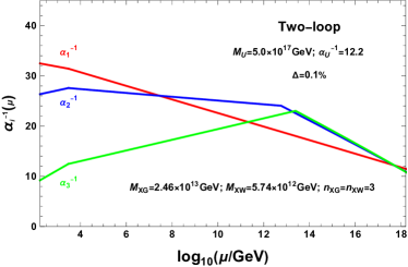
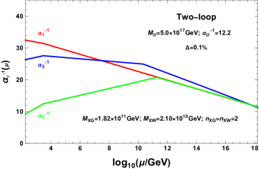
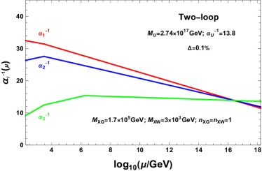
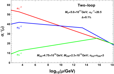
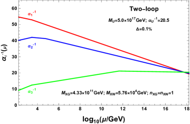
Figure 1: String-scale gauge coupling relations for Model 1 with XG+XWXG+XW. The number of added particle pairs is (a) 3, (b) 2, and (c) 1.
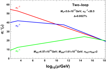
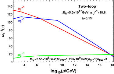
Figure 2: String-scale gauge coupling relations for Model 1-dual with XG+XWXG+XW. The number of added particle pairs is (a) 3, (b) 2, and (c) 1.

Following the conventions in refs. Chen et al. 2018; Chen et al. 2020; He et al. 2022a; Li et al. 2023 and taking the supersymmetry breaking scale at 33 TeV, the gauge couplings unify close to the string scale, 5×10175\times 10^{17} GeV. It is customary to redefine the set of parameters as,

α1kYgY2/4π,α2k2gb2/4π,α3ga2/4π.\alpha_{1}\equiv k_{Y}g_{Y}^{2}/4\pi,\quad\alpha_{2}\equiv k_{2}g_{b}^{2}/4\pi,\quad\alpha_{3}\equiv g_{a}^{2}/4\pi. (32)

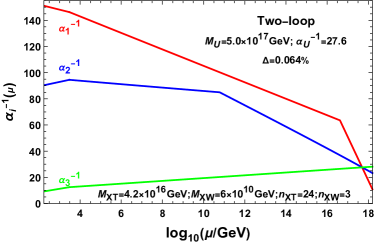
where kYk_{Y} is canonically chosen to be 5/35/3. In our calculations, the The string-scale gauge coupling relation in the evolution is realized via αU1α11=(α21+α31)/2\alpha_{\text{U}}^{-1}\equiv\alpha_{1}^{-1}=(\alpha_{2}^{-1}+\alpha_{3}^{-1})/2 and the deviation Δ=|α11α21|/α11\Delta=|\alpha_{1}^{-1}-\alpha_{2}^{-1}|/\alpha_{1}^{-1} is limited to within 0.1%.

Figure 3: String-scale gauge coupling relations for Model 3 (a) and Model 3-dual (b) with vector-like particles. (a) VV represents XD+XD¯XD+\overline{XD}, XU+XU¯XU+\overline{XU}, and XE+XE¯XE+\overline{XE}; (b) XTXT represents XT+XT¯XT+\overline{XT}.

For Model 1 and Model 1-dual we use XGXG and XWXW particles coming from the chiral adjoints associated with the special unitary group factors in the gauge group having the quantum numbers, XG=(𝟖,𝟏,𝟎)XG=(\mathbf{8,1,0}) and XW=(𝟏,𝟑,𝟎)XW=(\mathbf{1,3,0}), respectively. The one-loop contributions from these two particles to the beta function are Δb(XG)=(0,0,3)\Delta b(XG)=(0,0,3) and Δb(XW)=(0,2,0)\Delta b(XW)=(0,2,0) respectively Jiang et al. 2007; Barger et al. 2008. As the number of particles nXV(XV=XG,XW)n_{XV}(XV=XG,XW) increases, the mass of the particles MXVM_{XV} increases and the splitting between the XWXW and XGXG masses decreases.

In figure 1 and figure 2 we display the results of two-loop RGE running of the gauge couplings for Model 1 and Model 1-dual by adding 3 pairs, 2 pairs and 1 pair of XGXG and XWXW particles respectively. Above MXVM_{XV}, the running of SU(3)C{\rm SU}(3)_{C} coupling and SU(2)L{\rm SU}(2)_{L} coupling are reducing due to the non-zero beta functions Δb3(XG)\Delta b_{3}(XG) and Δb2(XW)\Delta b_{2}(XW).

Similarly in figure 3 we show the corresponding results of two-loop RGE running of the gauge couplings for Model 3 and Model 3-dual by adding vector-like particles. For the Model 3, the exotic particles are XD+XD¯XD+\overline{XD}, XU+XU¯XU+\overline{XU}, XE+XE¯XE+\overline{XE} and XWXW particles. Under the SU(3)C×SU(2)L×U(1)YSU(3)_{C}\times SU(2)_{L}\times U(1)_{Y} gauge symmetry, the corresponding quantum numbers and the contributions to one-loop level beta functions are

XD\displaystyle XD =(𝟑,𝟏,𝟏𝟑),\displaystyle=\mathbf{({3},1,-{1\over 3})}, XD¯\displaystyle\quad\overline{XD} =(𝟑¯,𝟏,𝟏𝟑),\displaystyle=\mathbf{({\bar{3}},1,{1\over 3})}, Δb\displaystyle\qquad\Delta b =(25,0,1);\displaystyle=({2\over 5},0,1)\,;
XU\displaystyle XU =(𝟑,𝟏,𝟐𝟑),\displaystyle=\mathbf{({3},1,{2\over 3})}, XU¯\displaystyle\quad\overline{XU} =(𝟑¯,𝟏,𝟐𝟑),\displaystyle=\mathbf{({\bar{3}},1,-{2\over 3})}, Δb\displaystyle\qquad\Delta b =(85,0,1);\displaystyle=({8\over 5},0,1)\,;
XE\displaystyle XE =(𝟏,𝟏,𝟏),\displaystyle=\mathbf{({1},1,{1})}, XE¯\displaystyle\quad\overline{XE} =(𝟏,𝟏,𝟏),\displaystyle=\mathbf{({1},1,-{1})}, Δb\displaystyle\qquad\Delta b =(65,0,0).\displaystyle=({6\over 5},0,0)\,. (33)

In the supersymmetric Pati-Salam models, these vector-like particles emerge from 𝒩=2{\cal N}=2 subsector intersections between aa and cc^{\prime} stacks of D6-brane. The number of these particles is thus nV=Iacn_{V}=I_{ac^{\prime}}. The XT+XT¯XT+\overline{XT} from cdcd and cdcd^{\prime} sectors are added to Model 3-dual to achieve the string-scale gauge coupling relations. The quantum numbers of XT+XT¯XT+\overline{XT} under the U(4)×USp(2)L×U(2)R×U(2)U(4)\times USp(2)_{L}\times U(2)_{R}\times U(2) gauge symmetry are (𝟏,𝟏,𝟐,𝟐,𝟏)+(𝟏,𝟏,𝟐,𝟐¯,𝟏)\mathbf{(1,1,2,2,1)+(1,1,2,\bar{2},1)}, and under the SU(3)C×SU(2)L×U(1)YSU(3)_{C}\times SU(2)_{L}\times U(1)_{Y} gauge symmetry are (𝟏,𝟏,𝟏𝟐)+(𝟏,𝟏,𝟏𝟐)\mathbf{(1,1,{1\over 2})+(1,1,-{1\over 2})}. The contributions to one-loop level beta functions are Δb=(65,0,0)\Delta b=({6\over 5},0,0). Since Icd=Icd=6I_{cd}=I_{cd^{\prime}}=6, we have 6×2×2=246\times 2\times 2=24 pairs of XT+XT¯XT+\overline{XT}. Therefore, we are able to show string-scale gauge coupling relations for each of the four chosen models.

V Discussion and conclusion

We have found new three-family supersymmetric Pati-Salam models with the gauge group SU(4)C×USp(2)L×SU(2)R{\rm SU}(4)_{C}\times{\rm USp}(2)_{L}\times{\rm SU}(2)_{R} on a 𝕋6/(2×2)\mathbbm{T}^{6}/(\mathbbm{Z}_{2}\times\mathbbm{Z}_{2}) orientifold from intersecting D6-branes at angles from the perspective of from IIA string theory without fluxes for the first time. Unlike the special unitary group, the symplectic group is a simpler choice as there is no associated global anomalous U(1) group. The unitary symplectic group arises by placing the D6-brane stack parallel to any of the four O6-planes. This seemingly minor change from SU(2) to USp(2) group is quite restrictive and drastically reduces the number of consistent three-family models. Therefore, while the number of three-family models with SU(4)C×SU(2)L×SU(2)R{\rm SU}(4)_{C}\times{\rm SU}(2)_{L}\times{\rm SU}(2)_{R} groups is found to be 202,752 He et al. 2022a; He et al. 2022b, the similar models by replacing either one of the SU(2) factors with a USp(2) is only 5. It is interesting to compare our search with ref. Cvetic et al. 2005 where one of us (TL) found only a single consistent three-family supersymmetric Pati-Salam model with the specific gauge group SU(4)C×USp(2)L×USp(2)R{\rm SU}(4)_{C}\times{\rm USp}(2)_{L}\times{\rm USp}(2)_{R}.

We have displayed the perturbative particle spectra of all the five inequivalent representative models and also discussed the duality under the exchange of the left and the right sectors. In particular, one of models (Model 1) does not contain any filler O6-planes whereas the other four models contain a single stack of filler branes each. The highest wrapping number is found to be 4 and all models contain extra exotic particles. We have shown the decoupling of such exotic particles originating from the hidden sector through the mechanism of strong coupling dynamics for the Model 3 and Model 3-dual. We have also calculated the tree-level gauge coupling relations for all models. By running the two-loop RGEs with the appropriate addition of SU(4)C{\rm SU}(4)_{C}/SU(2)L{\rm SU}(2)_{L} chiral adjoints and vector-like particle pairs, the gauge couplings are shown to be unified at the string-scale for some of the models.

Among the five models, the highest number of Higgs pairs is found to be 4 for Model 1 whereas all other models either contain a double or a single pair each. Thus, Model 1 may be the only viable candidate to explain the Yukawa couplings and fermion masses. However, we note that the two exotic symmetric representations corresponding to the SU(4)C{\rm SU}(4)_{C} group in Model 1 cannot be decoupled from the visible spectrum. It is Model 3 and Model 3-dual where all exotic states can be decoupled from the visible spectrum since there exist no exotic symmetric representations corresponding to the SU(4)C{\rm SU}(4)_{C} group. However, both Model 3 and Model 3-dual suffer from the rank-1 problem as the number of Higgs pair is only one each. In a related paper Mansha et al. 2023, we also discuss similar construction of supersymmetric Pati-Salam models with symplectic group from the perspective of possible hidden sector variations that can also affect the gauge coupling relations at the string-scale.

Acknowledgements.
TL is supported in part by the National Key Research and Development Program of China Grant No. 2020YFC2201504, by the Projects No. 11875062, No. 11947302, No. 12047503, and No. 12275333 supported by the National Natural Science Foundation of China, by the Key Research Program of the Chinese Academy of Sciences, Grant No. XDPB15, by the Scientific Instrument Developing Project of the Chinese Academy of Sciences, Grant No. YJKYYQ20190049, and by the International Partnership Program of Chinese Academy of Sciences for Grand Challenges, Grant No. 112311KYSB20210012. L Wu is supported in part by the Natural Science Basic Research Program of Shaanxi, Program No. 2024JC-YBMS-039.

Appendix A Three-family Pati-Salam models with a symplectic group

In this appendix, we list all representative three-family supersymmetric Pati-Salam models with a symplectic group obtained from random scanning method. a,b,c,da,b,c,d in the first column in every table represent the four stacks of D6-branes, respectively. Similarly, 1,2,3,41,2,3,4 in the first columns is a short-handed notation for the filler branes along the Ω\Omega{\cal R}, Ωω\Omega{\cal R}\omega, Ωθω\Omega{\cal R}\theta\omega and Ωθ\Omega{\cal R}\theta O6-planes, respectively. The second column in each table lists the numbers of D6-branes in the respective stack. In the third column we record the wrapping numbers of each D6-brane configuration. The rest of the columns record the intersection numbers between various stacks. For instance, in the bb column of table 12, from top to bottom, the numbers represent intersection numbers Iab,Ibc,IbdI_{ab},I_{bc},I_{bd}, etc. As usual, bb^{\prime} and cc^{\prime} are the orientifold Ω\Omega{\cal R} image of bb and cc stacks of D6-branes. We also list the relation between xA,xB,xC,xDx_{A},x_{B},x_{C},x_{D}, which are determined by the supersymmetry conditions (10), as well as the relation between the moduli parameter χ1,χ2,χ3\chi_{1},\,\chi_{2},\,\chi_{3}. The one loop beta functions βig\beta^{g}_{i} for each of the hidden sector stack is also listed. The gauge coupling relations are given in the caption of each table.

Table 12: D6-brane configurations and intersection numbers of Model 1, and its gauge coupling relation is ga2=87gb2=43gc2=65(53gY2)=327234πeϕ4g^{2}_{a}=\frac{8}{7}\,g^{2}_{b}=\frac{4}{3}\,g_{c}^{2}=\frac{6}{5}\,\left(\frac{5}{3}\,g^{2}_{Y}\right)=\frac{32}{7}\sqrt[4]{\frac{2}{3}}\,\pi\,e^{\phi_{4}}.
Model 1U(4)×USp(2)L×U(2)R×U(2)stackN(n1,l1)×(n2,l2)×(n3,l3)n


n                       bccdd1234
a8(1,3)×(0,1)×(1,1)22330440000b2(1,0)×(1,0)×(2,0)00-44220000c4(0,1)×(3,4)×(1,1)11---4100000d4(1,1)×(1,2)×(3,1)222-----0000βdg=8,xA=34xB=13xC=124xDχ1=6/18,χ2=6/8,χ3=26
\begin{array}[]{|c|c|c |r|r|r| r|r|r| r|r|r| r|r|r|}\hline\cr\vrule\lx@intercol\hfil\text{Model~\hyperref@@ii[model0]{1}}\hfil\lx@intercol\vrule\lx@intercol&\lx@intercol\hfil{\rm U}(4)\times{\rm USp}(2)_{L}\times{\rm U}(2)_{R}\times{\rm U}(2)\hfil\lx@intercol\vrule\lx@intercol\\ \hline\cr\hline\cr\rm{stack}&N&(n^{1},l^{1})\times(n^{2},l^{2})\times(n^{3},l^{3})&n_{\hskip 0.0pt{\vbox{\vbox{\hrule height=0.4pt\hbox{\vrule height=4.56001pt,width=0.4pt,depth=1.13998pt\hbox to5.70001pt{\hfil}\vrule height=4.56001pt,width=0.4pt,depth=1.13998pt\hbox to5.70001pt{\hfil}\vrule height=4.56001pt,width=0.4pt,depth=1.13998pt}\hrule height=0.4pt}\vskip-0.4pt}}\hskip 0.0pt}&n_{\hskip 0.0pt{\vbox{\vbox{\hrule height=0.4pt\hbox{\vrule height=4.56001pt,width=0.4pt,depth=1.13998pt\hbox to5.70001pt{\hfil}\vrule height=4.56001pt,width=0.4pt,depth=1.13998pt}\hrule height=0.4pt}\vskip-0.4pt\vbox{\hrule height=0.4pt\hbox{\vrule height=4.56001pt,width=0.4pt,depth=1.13998pt\hbox to5.70001pt{\hfil}\vrule height=4.56001pt,width=0.4pt,depth=1.13998pt}\hrule height=0.4pt}\vskip-0.4pt}}\hskip 0.0pt}&b&c&c^{\prime}&d&d^{\prime}&1&2&3&4\\ \hline\cr a&8&(-1,-3)\times(0,-1)\times(-1,-1)&-2&2&3&-3&0&4&4&0&0&0&0\\ b&2&(1,0)\times(1,0)\times(2,0)&0&0&\text{-}&4&-4&2&-2&0&0&0&0\\ c&4&(0,1)\times(3,-4)\times(1,-1)&1&-1&\text{-}&\text{-}&\text{-}&4&-10&0&0&0&0\\ d&4&(-1,1)\times(1,-2)\times(-3,-1)&-2&-22&\text{-}&\text{-}&\text{-}&\text{-}&\text{-}&0&0&0&0\\ \hline\cr&&&\lx@intercol\hfil\beta^{g}_{d}=8,\hskip 8.50012ptx_{A}=\frac{3}{4}x_{B}=\frac{1}{3}x_{C}=\frac{1}{24}x_{D}\hfil\lx@intercol\vrule\lx@intercol\\ &&&\lx@intercol\hfil\chi_{1}=\sqrt{6}/18,\hskip 8.50012pt\chi_{2}=\sqrt{6}/8,\hskip 8.50012pt\chi_{3}=2\sqrt{6}\hfil\lx@intercol\vrule\lx@intercol\\ \hline\cr\end{array}
Table 13: D6-brane configurations and intersection numbers of Model 1-dual, and its gauge coupling relation is ga2=43gb2=87gc2=3835(53gY2)=327234πeϕ4g^{2}_{a}=\frac{4}{3}\,g^{2}_{b}=\frac{8}{7}\,g_{c}^{2}=\frac{38}{35}\,\left(\frac{5}{3}\,g^{2}_{Y}\right)=\frac{32}{7}\sqrt[4]{\frac{2}{3}}\,\pi\,e^{\phi_{4}}.
Model 1-dualU(4)×U(2)L×USp(2)R×U(2)stackN(n1,l1)×(n2,l2)×(n3,l3)n


n                       bbcdd1234
a8(1,3)×(0,1)×(1,1)22303440000b4(0,1)×(3,4)×(1,1)11--44100000c2(1,0)×(1,0)×(2,0)00---220000d4(1,1)×(1,2)×(3,1)222-----0000βdg=8,xA=34xB=13xC=124xDχ1=6/18,χ2=6/8,χ3=26
\begin{array}[]{|c|c|c |r|r|r| r|r|r| r|r|r| r|r|r|}\hline\cr\vrule\lx@intercol\hfil\text{Model~\hyperref@@ii[model0dual]{1-dual}}\hfil\lx@intercol\vrule\lx@intercol&\lx@intercol\hfil{\rm U}(4)\times{\rm U}(2)_{L}\times{\rm USp}(2)_{R}\times{\rm U}(2)\hfil\lx@intercol\vrule\lx@intercol\\ \hline\cr\hline\cr\rm{stack}&N&(n^{1},l^{1})\times(n^{2},l^{2})\times(n^{3},l^{3})&n_{\hskip 0.0pt{\vbox{\vbox{\hrule height=0.4pt\hbox{\vrule height=4.56001pt,width=0.4pt,depth=1.13998pt\hbox to5.70001pt{\hfil}\vrule height=4.56001pt,width=0.4pt,depth=1.13998pt\hbox to5.70001pt{\hfil}\vrule height=4.56001pt,width=0.4pt,depth=1.13998pt}\hrule height=0.4pt}\vskip-0.4pt}}\hskip 0.0pt}&n_{\hskip 0.0pt{\vbox{\vbox{\hrule height=0.4pt\hbox{\vrule height=4.56001pt,width=0.4pt,depth=1.13998pt\hbox to5.70001pt{\hfil}\vrule height=4.56001pt,width=0.4pt,depth=1.13998pt}\hrule height=0.4pt}\vskip-0.4pt\vbox{\hrule height=0.4pt\hbox{\vrule height=4.56001pt,width=0.4pt,depth=1.13998pt\hbox to5.70001pt{\hfil}\vrule height=4.56001pt,width=0.4pt,depth=1.13998pt}\hrule height=0.4pt}\vskip-0.4pt}}\hskip 0.0pt}&b&b^{\prime}&c&d&d^{\prime}&1&2&3&4\\ \hline\cr a&8&(-1,-3)\times(0,-1)\times(-1,-1)&-2&2&-3&0&3&4&4&0&0&0&0\\ b&4&(0,1)\times(3,-4)\times(1,-1)&1&-1&\text{-}&\text{-}&-4&4&-10&0&0&0&0\\ c&2&(1,0)\times(1,0)\times(2,0)&0&0&\text{-}&\text{-}&\text{-}&2&-2&0&0&0&0\\ d&4&(-1,1)\times(1,-2)\times(-3,-1)&-2&-22&\text{-}&\text{-}&\text{-}&\text{-}&\text{-}&0&0&0&0\\ \hline\cr&&&\lx@intercol\hfil\beta^{g}_{d}=8,\hskip 8.50012ptx_{A}=\frac{3}{4}x_{B}=\frac{1}{3}x_{C}=\frac{1}{24}x_{D}\hfil\lx@intercol\vrule\lx@intercol\\ &&&\lx@intercol\hfil\chi_{1}=\sqrt{6}/18,\hskip 8.50012pt\chi_{2}=\sqrt{6}/8,\hskip 8.50012pt\chi_{3}=2\sqrt{6}\hfil\lx@intercol\vrule\lx@intercol\\ \hline\cr\end{array}
Table 14: D6-brane configurations and intersection numbers of Model 2, and its gauge coupling relation is ga2=1136gb2=13gc2=35(53gY2)=229113/4πeϕ4g^{2}_{a}=\frac{11}{36}\,g^{2}_{b}=\frac{1}{3}\,g_{c}^{2}=\frac{3}{5}\,\left(\frac{5}{3}\,g^{2}_{Y}\right)=\frac{2\sqrt{2}}{9}11^{3/4}\,\pi\,e^{\phi_{4}}.
Model2U(4)×USp(2)L×U(2)R×U(2)×USp(2)stackN(n1,l1)×(n2,l2)×(n3,l3)n


n                       bccdd1234
a8(1,3)×(1,0)×(1,1)22303440000b2(1,0)×(0,1)×(0,2)00-11110000c4(0,1)×(1,3)×(1,1)22---443000d4(1,1)×(1,1)×(1,3)012-----300012(1,0)×(1,0)×(2,0)βdg=7,β1g=0,xA=13xB=133xC=19xDχ1=11/33,χ2=11/3,χ3=211/11
\begin{array}[]{|c|c|c |r|r|r| r|r|r| r|r|r| r|r|r|}\hline\cr\vrule\lx@intercol\hfil\rm{Model~\hyperref@@ii[model2.1]{2}}\hfil\lx@intercol\vrule\lx@intercol&\lx@intercol\hfil{\rm U}(4)\times{\rm USp}(2)_{L}\times{\rm U}(2)_{R}\times{\rm U}(2)\times{\rm USp}(2)\hfil\lx@intercol\vrule\lx@intercol\\ \hline\cr\hline\cr\rm{stack}&N&(n^{1},l^{1})\times(n^{2},l^{2})\times(n^{3},l^{3})&n_{\hskip 0.0pt{\vbox{\vbox{\hrule height=0.4pt\hbox{\vrule height=4.56001pt,width=0.4pt,depth=1.13998pt\hbox to5.70001pt{\hfil}\vrule height=4.56001pt,width=0.4pt,depth=1.13998pt\hbox to5.70001pt{\hfil}\vrule height=4.56001pt,width=0.4pt,depth=1.13998pt}\hrule height=0.4pt}\vskip-0.4pt}}\hskip 0.0pt}&n_{\hskip 0.0pt{\vbox{\vbox{\hrule height=0.4pt\hbox{\vrule height=4.56001pt,width=0.4pt,depth=1.13998pt\hbox to5.70001pt{\hfil}\vrule height=4.56001pt,width=0.4pt,depth=1.13998pt}\hrule height=0.4pt}\vskip-0.4pt\vbox{\hrule height=0.4pt\hbox{\vrule height=4.56001pt,width=0.4pt,depth=1.13998pt\hbox to5.70001pt{\hfil}\vrule height=4.56001pt,width=0.4pt,depth=1.13998pt}\hrule height=0.4pt}\vskip-0.4pt}}\hskip 0.0pt}&b&c&c^{\prime}&d&d^{\prime}&1&2&3&4\\ \hline\cr a&8&(-1,-3)\times(-1,0)\times(1,-1)&-2&2&3&0&-3&4&4&0&0&0&0\\ b&2&(1,0)\times(0,1)\times(0,-2)&0&0&\text{-}&-1&1&1&-1&0&0&0&0\\ c&4&(0,1)\times(1,-3)\times(1,-1)&2&-2&\text{-}&\text{-}&\text{-}&4&-4&-3&0&0&0\\ d&4&(-1,1)\times(-1,-1)\times(1,-3)&0&-12&\text{-}&\text{-}&\text{-}&\text{-}&\text{-}&-3&0&0&0\\ \hline\cr 1&2&(1,0)\times(1,0)\times(2,0)&\lx@intercol\hfil\beta^{g}_{d}=7,~\beta^{g}_{1}=0,\hskip 8.50012ptx_{A}=\frac{1}{3}x_{B}=\frac{1}{33}x_{C}=\frac{1}{9}x_{D}\hfil\lx@intercol\vrule\lx@intercol\\ &&&\lx@intercol\hfil\chi_{1}=\sqrt{11}/33,\hskip 8.50012pt\chi_{2}=\sqrt{11}/3,\hskip 8.50012pt\chi_{3}=2\sqrt{11}/11\hfil\lx@intercol\vrule\lx@intercol\\ \hline\cr\end{array}
Table 15: D6-brane configurations and intersection numbers of Model 3, and its gauge coupling relation is ga2=518gb2=13gc2=35(53gY2)=42953/4πeϕ4g^{2}_{a}=\frac{5}{18}\,g^{2}_{b}=\frac{1}{3}\,g_{c}^{2}=\frac{3}{5}\,\left(\frac{5}{3}\,g^{2}_{Y}\right)=\frac{4\sqrt{2}}{9}5^{3/4}\,\pi\,e^{\phi_{4}}.
Model3U(4)×USp(2)L×U(2)R×U(2)×USp(2)stackN(n1,l1)×(n2,l2)×(n3,l3)n


n                       bccdd1234
a8(1,0)×(1,3)×(1,3)00330000000b2(0,1)×(1,0)×(0,2)00-11660000c4(1,1)×(0,1)×(1,3)22---300000d4(2,1)×(1,3)×(1,3)1656-----010022(1,0)×(0,1)×(0,2)βdg=3,β2g=5,xA=145xB=13xC=13xDχ1=5,χ2=5/15,χ3=25/15
\begin{array}[]{|c|c|c |r|r|r| r|r|r| r|r|r| r|r|r|}\hline\cr\vrule\lx@intercol\hfil\rm{Model~\hyperref@@ii[model2.2]{3}}\hfil\lx@intercol\vrule\lx@intercol&\lx@intercol\hfil{\rm U}(4)\times{\rm USp}(2)_{L}\times{\rm U}(2)_{R}\times{\rm U}(2)\times{\rm USp}(2)\hfil\lx@intercol\vrule\lx@intercol\\ \hline\cr\hline\cr\rm{stack}&N&(n^{1},l^{1})\times(n^{2},l^{2})\times(n^{3},l^{3})&n_{\hskip 0.0pt{\vbox{\vbox{\hrule height=0.4pt\hbox{\vrule height=4.56001pt,width=0.4pt,depth=1.13998pt\hbox to5.70001pt{\hfil}\vrule height=4.56001pt,width=0.4pt,depth=1.13998pt\hbox to5.70001pt{\hfil}\vrule height=4.56001pt,width=0.4pt,depth=1.13998pt}\hrule height=0.4pt}\vskip-0.4pt}}\hskip 0.0pt}&n_{\hskip 0.0pt{\vbox{\vbox{\hrule height=0.4pt\hbox{\vrule height=4.56001pt,width=0.4pt,depth=1.13998pt\hbox to5.70001pt{\hfil}\vrule height=4.56001pt,width=0.4pt,depth=1.13998pt}\hrule height=0.4pt}\vskip-0.4pt\vbox{\hrule height=0.4pt\hbox{\vrule height=4.56001pt,width=0.4pt,depth=1.13998pt\hbox to5.70001pt{\hfil}\vrule height=4.56001pt,width=0.4pt,depth=1.13998pt}\hrule height=0.4pt}\vskip-0.4pt}}\hskip 0.0pt}&b&c&c^{\prime}&d&d^{\prime}&1&2&3&4\\ \hline\cr a&8&(-1,0)\times(-1,-3)\times(1,-3)&0&0&3&-3&0&0&0&0&0&0&0\\ b&2&(0,1)\times(1,0)\times(0,-2)&0&0&\text{-}&1&-1&6&-6&0&0&0&0\\ c&4&(1,1)\times(0,1)\times(-1,-3)&-2&2&\text{-}&\text{-}&\text{-}&3&0&0&0&0&0\\ d&4&(2,1)\times(1,-3)\times(1,-3)&-16&-56&\text{-}&\text{-}&\text{-}&\text{-}&\text{-}&0&1&0&0\\ \hline\cr 2&2&(1,0)\times(0,-1)\times(0,2)&\lx@intercol\hfil\beta^{g}_{d}=3,~\beta^{g}_{2}=-5,\hskip 8.50012ptx_{A}=\frac{1}{45}x_{B}=\frac{1}{3}x_{C}=\frac{1}{3}x_{D}\hfil\lx@intercol\vrule\lx@intercol\\ &&&\lx@intercol\hfil\chi_{1}=\sqrt{5},\hskip 8.50012pt\chi_{2}=\sqrt{5}/15,\hskip 8.50012pt\chi_{3}=2\sqrt{5}/15\hfil\lx@intercol\vrule\lx@intercol\\ \hline\cr\end{array}
Table 16: D6-brane configurations and intersection numbers of Model 3-dual, and its gauge coupling relation is ga2=13gb2=518gc2=1730(53gY2)=42953/4πeϕ4g^{2}_{a}=\frac{1}{3}\,g^{2}_{b}=\frac{5}{18}\,g_{c}^{2}=\frac{17}{30}\,\left(\frac{5}{3}\,g^{2}_{Y}\right)=\frac{4\sqrt{2}}{9}5^{3/4}\,\pi\,e^{\phi_{4}}.
Model 3-dualU(4)×U(2)L×USp(2)R×U(2)×USp(2)stackN(n1,l1)×(n2,l2)×(n3,l3)n


n                       bbcdd1234
a8(1,0)×(1,3)×(1,3)00303000000b4(1,1)×(0,1)×(1,3)22--1300000c2(0,1)×(1,0)×(0,2)00---660000d4(2,1)×(1,3)×(1,3)1656-----010022(1,0)×(0,1)×(0,2)βdg=3,β2g=5,xA=145xB=13xC=13xDχ1=5,χ2=5/15,χ3=25/15
\begin{array}[]{|c|c|c |r|r|r| r|r|r| r|r|r| r|r|r|}\hline\cr\vrule\lx@intercol\hfil\text{Model~\hyperref@@ii[model2.2dual]{3-dual}}\hfil\lx@intercol\vrule\lx@intercol&\lx@intercol\hfil{\rm U}(4)\times{\rm U}(2)_{L}\times{\rm USp}(2)_{R}\times{\rm U}(2)\times{\rm USp}(2)\hfil\lx@intercol\vrule\lx@intercol\\ \hline\cr\hline\cr\rm{stack}&N&(n^{1},l^{1})\times(n^{2},l^{2})\times(n^{3},l^{3})&n_{\hskip 0.0pt{\vbox{\vbox{\hrule height=0.4pt\hbox{\vrule height=4.56001pt,width=0.4pt,depth=1.13998pt\hbox to5.70001pt{\hfil}\vrule height=4.56001pt,width=0.4pt,depth=1.13998pt\hbox to5.70001pt{\hfil}\vrule height=4.56001pt,width=0.4pt,depth=1.13998pt}\hrule height=0.4pt}\vskip-0.4pt}}\hskip 0.0pt}&n_{\hskip 0.0pt{\vbox{\vbox{\hrule height=0.4pt\hbox{\vrule height=4.56001pt,width=0.4pt,depth=1.13998pt\hbox to5.70001pt{\hfil}\vrule height=4.56001pt,width=0.4pt,depth=1.13998pt}\hrule height=0.4pt}\vskip-0.4pt\vbox{\hrule height=0.4pt\hbox{\vrule height=4.56001pt,width=0.4pt,depth=1.13998pt\hbox to5.70001pt{\hfil}\vrule height=4.56001pt,width=0.4pt,depth=1.13998pt}\hrule height=0.4pt}\vskip-0.4pt}}\hskip 0.0pt}&b&b^{\prime}&c&d&d^{\prime}&1&2&3&4\\ \hline\cr a&8&(-1,0)\times(-1,-3)\times(1,-3)&0&0&-3&0&3&0&0&0&0&0&0\\ b&4&(1,1)\times(0,1)\times(-1,-3)&-2&2&\text{-}&\text{-}&-1&3&0&0&0&0&0\\ c&2&(0,1)\times(1,0)\times(0,-2)&0&0&\text{-}&\text{-}&\text{-}&6&-6&0&0&0&0\\ d&4&(2,1)\times(1,-3)\times(1,-3)&-16&-56&\text{-}&\text{-}&\text{-}&\text{-}&\text{-}&0&1&0&0\\ \hline\cr 2&2&(1,0)\times(0,-1)\times(0,2)&\lx@intercol\hfil\beta^{g}_{d}=3,~\beta^{g}_{2}=-5,\hskip 8.50012ptx_{A}=\frac{1}{45}x_{B}=\frac{1}{3}x_{C}=\frac{1}{3}x_{D}\hfil\lx@intercol\vrule\lx@intercol\\ &&&\lx@intercol\hfil\chi_{1}=\sqrt{5},\hskip 8.50012pt\chi_{2}=\sqrt{5}/15,\hskip 8.50012pt\chi_{3}=2\sqrt{5}/15\hfil\lx@intercol\vrule\lx@intercol\\ \hline\cr\end{array}
Table 17: D6-brane configurations and intersection numbers of Model 4, and its gauge coupling relation is ga2=1118gb2=23gc2=45(53gY2)=49 113/4πeϕ4g^{2}_{a}=\frac{11}{18}\,g^{2}_{b}=\frac{2}{3}\,g_{c}^{2}=\frac{4}{5}\,\left(\frac{5}{3}\,g^{2}_{Y}\right)=\frac{4}{9}\,11^{3/4}\,\pi\,e^{\phi_{4}}.
Model4U(4)×USp(2)L×U(2)R×U(2)×USp(4)stackN(n1,l1)×(n2,l2)×(n3,l3)n


n                       bccdd1234
a8(1,0)×(1,3)×(1,1)22330440000b2(0,1)×(1,0)×(0,2)00-22220000c4(2,3)×(0,1)×(1,1)11---880000d4(2,1)×(1,1)×(1,3)222-----010024(1,0)×(0,1)×(0,2)βdg=12,β2g=5,xA=133xB=23xC=29xDχ1=211/3,χ2=11/33,χ3=211/11
\begin{array}[]{|c|c|c |r|r|r| r|r|r| r|r|r| r|r|r|}\hline\cr\vrule\lx@intercol\hfil\rm{Model~\hyperref@@ii[model4]{4}}\hfil\lx@intercol\vrule\lx@intercol&\lx@intercol\hfil{\rm U}(4)\times{\rm USp}(2)_{L}\times{\rm U}(2)_{R}\times{\rm U}(2)\times{\rm USp}(4)\hfil\lx@intercol\vrule\lx@intercol\\ \hline\cr\hline\cr\rm{stack}&N&(n^{1},l^{1})\times(n^{2},l^{2})\times(n^{3},l^{3})&n_{\hskip 0.0pt{\vbox{\vbox{\hrule height=0.4pt\hbox{\vrule height=4.56001pt,width=0.4pt,depth=1.13998pt\hbox to5.70001pt{\hfil}\vrule height=4.56001pt,width=0.4pt,depth=1.13998pt\hbox to5.70001pt{\hfil}\vrule height=4.56001pt,width=0.4pt,depth=1.13998pt}\hrule height=0.4pt}\vskip-0.4pt}}\hskip 0.0pt}&n_{\hskip 0.0pt{\vbox{\vbox{\hrule height=0.4pt\hbox{\vrule height=4.56001pt,width=0.4pt,depth=1.13998pt\hbox to5.70001pt{\hfil}\vrule height=4.56001pt,width=0.4pt,depth=1.13998pt}\hrule height=0.4pt}\vskip-0.4pt\vbox{\hrule height=0.4pt\hbox{\vrule height=4.56001pt,width=0.4pt,depth=1.13998pt\hbox to5.70001pt{\hfil}\vrule height=4.56001pt,width=0.4pt,depth=1.13998pt}\hrule height=0.4pt}\vskip-0.4pt}}\hskip 0.0pt}&b&c&c^{\prime}&d&d^{\prime}&1&2&3&4\\ \hline\cr a&8&(-1,0)\times(-1,-3)\times(1,-1)&-2&2&3&-3&0&4&4&0&0&0&0\\ b&2&(0,1)\times(1,0)\times(0,-2)&0&0&\text{-}&2&-2&2&-2&0&0&0&0\\ c&4&(2,3)\times(0,1)\times(-1,-1)&-1&1&\text{-}&\text{-}&\text{-}&8&-8&0&0&0&0\\ d&4&(2,1)\times(1,-1)\times(1,-3)&-2&-22&\text{-}&\text{-}&\text{-}&\text{-}&\text{-}&0&1&0&0\\ \hline\cr 2&4&(1,0)\times(0,-1)\times(0,2)&\lx@intercol\hfil\beta^{g}_{d}=12,~\beta^{g}_{2}=-5,\hskip 8.50012ptx_{A}=\frac{1}{33}x_{B}=\frac{2}{3}x_{C}=\frac{2}{9}x_{D}\hfil\lx@intercol\vrule\lx@intercol\\ &&&\lx@intercol\hfil\chi_{1}=2\sqrt{11}/3,\hskip 8.50012pt\chi_{2}=\sqrt{11}/33,\hskip 8.50012pt\chi_{3}=2\sqrt{11}/11\hfil\lx@intercol\vrule\lx@intercol\\ \hline\cr\end{array}
Table 18: D6-brane configurations and intersection numbers of Model 5, and its gauge coupling relation is ga2=722gb2=13gc2=35(53gY2)=421173/434πeϕ4g^{2}_{a}=\frac{7}{22}\,g^{2}_{b}=\frac{1}{3}\,g_{c}^{2}=\frac{3}{5}\,\left(\frac{5}{3}\,g^{2}_{Y}\right)=\frac{4\sqrt{2}}{11}\frac{7^{3/4}}{\sqrt[4]{3}}\,\pi\,e^{\phi_{4}}.
Model5U(4)×USp(2)L×U(2)R×U(2)×USp(6)stackN(n1,l1)×(n2,l2)×(n3,l3)n


n                       bccdd1234
a8(1,3)×(1,0)×(1,1)22303440000b2(1,0)×(0,1)×(0,2)00-11220000c4(0,1)×(1,3)×(1,1)22---7100000d4(1,1)×(2,1)×(1,3)222-----001036(0,1)×(1,0)×(0,2)βdg=11,β3g=5,xA=13xB=163xC=19xDχ1=21/63,χ2=21/3,χ3=22/21
\begin{array}[]{|c|c|c |r|r|r| r|r|r| r|r|r| r|r|r|}\hline\cr\vrule\lx@intercol\hfil\rm{Model~\hyperref@@ii[model6]{5}}\hfil\lx@intercol\vrule\lx@intercol&\lx@intercol\hfil{\rm U}(4)\times{\rm USp}(2)_{L}\times{\rm U}(2)_{R}\times{\rm U}(2)\times{\rm USp}(6)\hfil\lx@intercol\vrule\lx@intercol\\ \hline\cr\hline\cr\rm{stack}&N&(n^{1},l^{1})\times(n^{2},l^{2})\times(n^{3},l^{3})&n_{\hskip 0.0pt{\vbox{\vbox{\hrule height=0.4pt\hbox{\vrule height=4.56001pt,width=0.4pt,depth=1.13998pt\hbox to5.70001pt{\hfil}\vrule height=4.56001pt,width=0.4pt,depth=1.13998pt\hbox to5.70001pt{\hfil}\vrule height=4.56001pt,width=0.4pt,depth=1.13998pt}\hrule height=0.4pt}\vskip-0.4pt}}\hskip 0.0pt}&n_{\hskip 0.0pt{\vbox{\vbox{\hrule height=0.4pt\hbox{\vrule height=4.56001pt,width=0.4pt,depth=1.13998pt\hbox to5.70001pt{\hfil}\vrule height=4.56001pt,width=0.4pt,depth=1.13998pt}\hrule height=0.4pt}\vskip-0.4pt\vbox{\hrule height=0.4pt\hbox{\vrule height=4.56001pt,width=0.4pt,depth=1.13998pt\hbox to5.70001pt{\hfil}\vrule height=4.56001pt,width=0.4pt,depth=1.13998pt}\hrule height=0.4pt}\vskip-0.4pt}}\hskip 0.0pt}&b&c&c^{\prime}&d&d^{\prime}&1&2&3&4\\ \hline\cr a&8&(1,3)\times(1,0)\times(1,-1)&-2&2&3&0&-3&4&4&0&0&0&0\\ b&2&(1,0)\times(0,1)\times(0,-2)&0&0&\text{-}&-1&1&2&-2&0&0&0&0\\ c&4&(0,-1)\times(-1,3)\times(1,-1)&2&-2&\text{-}&\text{-}&\text{-}&7&-10&0&0&0&0\\ d&4&(1,-1)\times(2,1)\times(1,-3)&-2&-22&\text{-}&\text{-}&\text{-}&\text{-}&\text{-}&0&0&1&0\\ \hline\cr 3&6&(0,-1)\times(1,0)\times(0,2)&\lx@intercol\hfil\beta^{g}_{d}=11,~\beta^{g}_{3}=-5,\hskip 8.50012ptx_{A}=\frac{1}{3}x_{B}=\frac{1}{63}x_{C}=\frac{1}{9}x_{D}\hfil\lx@intercol\vrule\lx@intercol\\ &&&\lx@intercol\hfil\chi_{1}=\sqrt{21}/63,\hskip 8.50012pt\chi_{2}=\sqrt{21}/3,\hskip 8.50012pt\chi_{3}=2\sqrt{2}/21\hfil\lx@intercol\vrule\lx@intercol\\ \hline\cr\end{array}

References