On the synchronization of the Kuramoto-type model of oscillators with lossy couplings

Abstract

We consider the problem of synchronization of coupled oscillators in a Kuramoto-type model with lossy couplings. Kuramoto models have been used to gain insight on the stability of power networks which are usually nonlinear and involve large scale interconnections. Such models commonly assume lossless couplings and Lyapunov functions have predominantly been employed to prove stability. However, coupling conductances can impact synchronization. We therefore consider a more advanced Kuramoto model that includes coupling conductances, and is characterized by nonhomogeneous coupling weights and noncomplete coupling graphs. Lyapunov analysis once such coupling conductances and aforementioned properties are included becomes nontrivial and more conventional energy-like Lyapunov functions are not applicable or are conservative. Small-signal analysis has been performed for such models, but due to the fact that we have convergence to a manifold, stability analysis via a linearization is on its own inconclusive for the nonlinear model. In this paper, we provide a formal derivation using centre manifold theory that if a particular condition on the equilibrium point associated with the coupling conductances and susceptances holds, then the synchronization manifold for the nonlinear system considered is asymptotically stable. Our analysis is demonstrated with simulations.

I Introduction

Stability analysis of power networks is a problem that has received a considerable amount of attention. Power networks are generally a complex interconnection of subsystems that include also nonlinear dynamics. These include controllable inverter-based microgrids which have been identified to offer good prospects for the integration of renewable energy sources in future grids. Considering the nonlinear and complex dynamics associated with power systems, simple models which are valid on slow timescales have been used to gain insight into the stability of their synchronized motion. Such a model is the Kuramoto model of coupled oscillators [1]. This was initially used to study chemical oscillators [1], and has since been employed in investigating the stability of power networks [2, 3, 4] as well as consensus protocols of multi-agent systems [5, 6]. Generally, Kuramoto models can be classified into the first-order type [7, 8, 9, 10, 3] and second-order type [2, 4].

The stability problem of coupled oscillators in Kuramoto models is a particular form of a synchronization problem. This is characterized by the synchronization of the frequencies of coupled oscillators to a common constant value. For power networks, this implies that the frequency of the generators (inverters) converge to a synchronous value. The synchronization of coupled Kuramoto oscillators has been widely reported in the literature, e.g. [7, 8, 9, 10] and with particular application to inverter-based microgrids [3, 4].

Kuramoto-type models have been used in the literature to provide intuition on the behaviour of power networks at slow timescales, by providing analytical results that hold in general network topologies. Such models have commonly been used to describe oscillators interconnected via lossless couplings [7, 8, 9, 10, 3], and thus the analysis of these Kuramoto-type models has been predominantly performed via Lyapunov functions. However, the line conductances (or resistances) in e.g. inverter-based grids are important as they can inhibit synchronization. Also, these power networks are usually characterized by nonhomogeneous coupling weights and noncomplete coupling graphs. Hence, here we consider a more advanced Kuramoto model that includes coupling conductances together with heterogeneous coupling weights and noncomplete coupling graphs, in contrast to those in e.g. [8, 7, 11]. Lyapunov analysis once such conductances and aforementioned coupling properties are included becomes nontrivial as more conventional energy-like Lyapunov functions are not applicable or are conservative, as reported in [2]. Small-signal analysis for this case exists in the literature, e.g [4]; however, since the system converges to a manifold a small-signal analysis is on its own inconclusive for the nonlinear system [12].

In this paper, we study the stability of the system using centre manifold theory [12, 13, 14]. Centre manifold theory allows to study the stability of nonlinear systems when linearization fails [12]. Using this theory, we provide a formal derivation that if a particular condition involving the coupling conductances and susceptances of the lossy Kuramoto-type model holds at an equilibrium point, the synchronization manifold for the system considered is asymptotically stable. A numerical example is also provided to demonstrate the results of our analysis.

The remainder of the paper is organized as follows. Preliminaries and the problem setup are given in section II. Section III presents our main results. A simulation example is given in section IV and conclusions are drawn in section V.

II Preliminaries and Problem Setup

Let $\mathbb{R}_{\geq 0}=\{x\in\mathbb{R}|x\geq 0\}$, $\mathbb{R}_{>0}=\{x\in\mathbb{R}|x>0\}$. We denote by $\mathbf{1}_{n}$ $(\mathbf{0}_{n})$ the $n$-dimensional column vector of ones (zeros), and $\mathbf{I}_{n}$ is the identity matrix of size $n$, and $\mathbf{j}$ a complex number. Given an $n$-tuple $(x_{1},\ldots,x_{n})$, $x=\text{col}(x_{i})\in\mathbb{R}^{n}$ is a column vector, $\text{diag}(x_{i})\in\mathbb{R}^{n\times n}$ is an $n\times n$ diagonal matrix, and $\|x\|$ denotes the 2-norm of $x$ and $\|x\|_{\infty}$ its infinity norm. Given $A\in\mathbb{R}^{n\times m}$, let $A^{\top}$ denote its transpose. Let $\mathbb{T}^{1}:=[-\pi,\pi]$, a phase angle $\delta_{i}$ is a point $\delta_{i}\in\mathbb{T}^{1}$, and an arc with length $\gamma$ is a connected subset of $\mathbb{T}^{1}$.

II-A Graph theory

We denote a directed graph by $\mathcal{G}=(\mathcal{V},\mathcal{E})$, where $\mathcal{V}=\{1,2,\ldots,N\},\,N=|\mathcal{V}|$ is the set of vertices (nodes), and $\mathcal{E}\subseteq\mathcal{V}\times\mathcal{V}$ is the set of directed edges with $E=|\mathcal{E}|$. Node $j\in\mathcal{V}$ is a neighbour of a node $i\in\mathcal{V}$ if $(i,j)\in\mathcal{E}$, and the set of neighbours of a node $i\in\mathcal{V}$ is denoted by $\mathcal{N}_{i}$. For each edge $(i,j)\in\mathcal{E}$, a number $z\in\{1,\ldots,E\}$ and an arbitrary direction are assigned and the entries of the incidence matrix $\mathcal{B}\in\mathbb{R}^{N\times E}$ are defined as $\mathcal{B}_{iz}=1$ if node $i$ is the source of edge $z$ and $\mathcal{B}_{iz}=-1$ if node $i$ is the sink of edge $z$, with all other elements being zero. Let the graph $\mathcal{G}$ be connected, i.e. for all $i,j\in\mathcal{V}$, there exists a path from $i$ to $j$. Hence, $\text{span}(\mathbf{1}_{N})\in\ker(\mathcal{B}^{\top})$. Let ${\mathbf{\hat{B}}}\in\mathbb{R}^{N\times E}$ be the element-wise absolute value of $\mathcal{B}$.

II-B Problem setup

We consider in this paper a Kuramoto-type model that takes coupling conductances into account. This is briefly described as follows ([2] can be consulted for an analogous derivation from first principles). Let the interconnection of the oscillators be described by the connected graph $\mathcal{G}$. Let each oscillator and load be connected at each node $i\in\mathcal{V}$, and the coupling between every node pair $(i,j)\in\mathcal{E}$ be characterized by an admittance $Y_{ij}=G_{ij}+\mathbf{j}B_{ij}$, where $G_{ij},B_{ij}\in\mathbb{R}_{>{0}}$ are the coupling conductance (losses) and susceptance respectively. Note that in the case of nodes to which only loads are connected, these can be eliminated using Kron-reduction [15, 16] leading to a lower dimensional representation of the original model where each node has an oscillator connected to it. We define

$$\begin{matrix}&\varpi_{i}=P^{d}_{i}-P_{L_{i}}-\sum_{j\in\mathcal{N}_{i}}G_{ij}V^{2}_{i},\\ &a_{ij}=V_{i}V_{j}G_{ij},~{}~{}b_{ij}=V_{i}V_{j}B_{ij},~{}~{}\delta_{ij}(t)=\delta_{i}(t)-\delta_{j}(t),\vspace{-0.125cm}\end{matrix}$$ (1)

where $V_{i},V_{j}\in\mathbb{R}_{>0}$ are the internal voltages of the oscillators at nodes $i,j$; $a_{ij}$, $b_{ij}\in\mathbb{R}_{>0}$ are respectively the lossy and lossless coupling weights; $P^{d}_{i},P_{L_{i}}\in\mathbb{R}_{>0}$ are respectively the desired power injection and the constant power load at a node $i$; and $\varpi_{i}$ denotes the effective power injection at node $i$ which is often referred to in Kuramoto models as the natural frequency [2] at that node. Variables $\delta_{i}(t),\delta_{j}(t)\in\mathbb{T}^{1}$ denote the phase angle of the oscillators at node $i$ and $j$, respectively; $\delta_{ij}(t)$ is the phase difference between the node pair $(i,j)\in\mathcal{E}$. Therefore, the dynamics of the Kuramoto model considered in this paper describing the interconnection of oscillators via lossy couplings are given by

$$\dot{\delta}_{i}(t)=k_{pi}\varpi_{i}-k_{pi}\displaystyle\sum_{j\in\mathcal{N}_{i}}(b_{ij}\sin(\delta_{ij}(t))-a_{ij}\cos(\delta_{ij}(t)))\vspace{-0.125cm}$$ (2)

for all $i\in\mathcal{V}$, with gain $k_{pi}\in\mathbb{R}_{>0}$. Note that the coupling weights $a_{ij},b_{ij}$ in (2) are allowed to be nonhomogeneous, i.e. the weights are not necessarily the same for every edge $(i,j)\in\mathcal{E}$ (as assumed in e.g. [8, 7, 11]). Also, each node is not required to be connected to all other nodes, i.e. each node $i\in\mathcal{V}$ connects to its neighbouring nodes $j\in\mathcal{N}_{i}$ where $\mathcal{N}_{i}\subset\mathcal{V}$. Furthermore, the term $a_{ij}$ being associated with the coupling conductance $G_{ij}$ in (1) allows the Kuramoto-type model (2) to take into account the coupling losses. Model (2) is also referred to as a first-order Kuramoto-type model.

Note that $a_{ij}$, $b_{ij}$ are respectively associated with the coupling conductance $G_{ij}$ and susceptance $B_{ij}$. Thus the term $b_{ij}\sin(\delta_{ij}(t))$ usually enables synchronization given its negative feedback role in (2) while $a_{ij}\cos(\delta_{ij}(t))$ can inhibit synchronization due to its positive feedback role in (2).

Remark 1

System (2) is a simplified model relevant for studying inverter-based power networks at slower timescales [3, 17]. This can be related to such networks as follows. Let $V_{i},V_{j}$ denote the inverter voltages at the corresponding buses and the couplings represented by power lines with conductances $G_{ij}$ and susceptances $B_{ij}$. The phase angle $\delta_{i}(t)$ is associated with the angle at each bus, and its derivative is defined as the deviation between the local frequency $\omega_{i}(t)\in\mathbb{R}_{>0}$ and a common frequency $\omega_{0}\in\mathbb{R}_{>0}$ [17], i.e., $\dot{\delta}_{i}(t)=\omega_{i}(t)-\omega_{0}:=u_{i}^{\omega}(t),\,\forall i\in\mathcal{V}$. Suppose the control input $u_{i}^{\omega}(t)$ is generated via a droop law $u_{i}^{\omega}(t)=-k_{pi}(P_{i}(t)-P^{d}_{i})$ [17] where the gain $k_{p_{i}}\in\mathbb{R}_{>0}$ is now the droop gain, and $P_{i}(t)\in\mathbb{R}_{>0}$ is the overall active power injection at a node $i\in\mathcal{V}$ given by [15, 17, 18] $P_{i}(t)=P_{L_{i}}+\sum_{j\in\mathcal{N}_{i}}[G_{ij}V^{2}_{i}-G_{ij}V_{i}V_{j}\cos(\delta_{i}(t)-\delta_{j}(t))+B_{ij}V_{i}V_{j}\sin(\delta_{i}(t)-\delta_{j}(t))]$. Then setting $\dot{\delta}_{i}(t):=u_{i}^{\omega}(t)$ leads to the Kuramoto-type model in (2).

In the subsequent analysis, we use (2) to investigate the synchronization of the coupled oscillators.

We note that in the remainder of this paper, the arguments $t$ of all signals are omitted to simplify the notation.

III Main Results

We present in this section our main results. In particular, using centre manifold theory we show that if a particular condition associated with the line conductances and susceptances is satisfied by an equilibrium point, then local asymptotic stability of the corresponding synchronization manifold holds.

To this end, we recall the definitions for frequency synchronization (Definition 1) and the synchronization (Definition 2) set that will be considered in our analysis.

Definition 1 (Frequency synchronization)

Let $\delta=\text{col}(\delta_{i})\in\mathbb{T}^{n}$. The oscillators in (2) have achieved synchronization if there exists a constant frequency deviation $\dot{\delta}_{\text{syn}}$ such that $\dot{\delta}(t)=\mathbf{1}_{N}{\color[rgb]{0,0,0}\dot{\delta}_{\text{syn}}}$.

Definition 2 (Synchronization set [2])

For some $\gamma\in[0,\pi/2-\psi_{\max})$, $\psi_{\max}=\max_{(i,j)\in\mathcal{E}}\arctan(G_{ij}/B_{ij})$, we define the set $\mathcal{C}(\gamma){:=}\{\delta:\|\mathcal{B}^{\top}\delta\|_{\infty}\leq\gamma\}\subset\mathbb{T}^{n}$, i.e. this is the closed set of angles $\delta=\text{col}(\delta_{1},\ldots,\delta_{N})$ with any neighbouring angle pair $\delta_{ij},\,\forall(i,j)\in\mathcal{E}$, no further than $\gamma$ apart.

Before presenting our main result on the synchronization of system (2), we illustrate the limitations of existing approaches when considering lossy interconnections. For lossless interconnections, i.e. $a_{ij}=0$, the only trigonometric term that appears in (2) is $b_{ij}\sin(\delta_{ij})$. This term has the property $b_{ij}\sin(\delta_{ij})=-b_{ij}\sin(\delta_{ji})$ which allows to find Lyapunov functions and simplifies significantly the analysis. However, this property is not satisfied by the other term $a_{ij}\cos(\delta_{ij})$ which is associated with $G_{ij}$. The nonhomogeneous parameters and noncomplete interconnection graph in (2) further complicates the analysis, and Lyapunov analysis once coupling conductances $G_{ij}$ are included can be conservative [4].

Theorem 1 is therefore based on a different approach, whereby the centre manifold theorem is used to analyze the stability properties of the nonlinear system. In particular, we show that the synchronization manifold for system (2) is locally asymptotically stable if a particular condition associated with the line conductances and susceptances is satisfied at an equilibrium point.

Theorem 1 (Frequency synchronization)

Consider system (2), together with (1). Assume there exists an equilibrium point $\delta^{*}$ that satisfies $\delta^{*}\in\mathcal{C}(\gamma)$ for some $\gamma\in[0,\pi/2-\psi_{\max})$ with $\psi_{\max}=\max_{(i,j)\in\mathcal{E}}\arctan(G_{ij}/B_{ij})$, and consider the manifold

$${\color[rgb]{0,0,0}{\mathcal{Y}_{\delta^{*}}=\left\{\delta^{*}+\delta_{0}\mathbf{1}_{N}{\color[rgb]{0,0,0}\ |\ \delta_{0}\in\mathbb{T}^{1}}\right\}.}}\vspace{-0.125cm}$$ (3)

Then the synchronization manifold $\mathcal{Y}_{\delta^{*}}$ is locally asymptotically stable. Furthermore, there exists a neighbourhood $\Xi$ of $\mathcal{Y}_{\delta^{*}}$ such that for every $\delta(0)\in\Xi$, $\lim_{t\to\infty}\|\delta(t)-\delta^{\dagger}\|\to 0$ for some $\delta^{\dagger}\in\mathcal{Y}_{\delta^{*}}$.

The proof can be found in Appendix A.

Remark 2

Using the centre manifold theorem, Theorem 1 shows that the synchronization manifold for the lossy case (2) is asymptotically stable for an equilibrium point $\delta^{*}$ that satisfies a condition associated with the line conductances and susceptances, i.e. for $\delta^{*}\in\mathcal{C}(\gamma)$ for some $\gamma\in[0,\pi/2-\psi_{\max})$ with $\psi_{\max}=\max_{(i,j)\in\mathcal{E}}\arctan(G_{ij}/B_{ij})$. This is a condition analogous to that for the lossless case e.g. [7, 8, 9, 19, 10] where Lyapunov analysis is used to show asymptotic stability for an equilibrium point $\delta^{*}\in\mathcal{C}(\gamma)$ with $\gamma\in[0,\pi/2)$.

Remark 3

We would like to note that system (2) has the following equivalent representation (stated as Lemma 1 in Appendix D).

$$\dot{\delta}_{i}=k_{pi}\varpi_{i}-k_{pi}\sum_{j\in\mathcal{N}_{i}}\sqrt{a^{2}_{ij}+b^{2}_{ij}}\,\sin(\delta_{ij}-\psi_{ij}),\hskip 5.69054pt\forall i\in\mathcal{V}\vspace{-0.125cm}$$ (4)

where $\psi_{ij}=\arctan(a_{ij}/b_{ij})=\arctan(G_{ij}/B_{ij})$. Therefore $\psi_{ij}$ correspond to phase shifts and $\psi_{\max}$ used in Theorem 1 is the maximum of these phase shifts. Since $G_{ij},B_{ij}>0$ (or $a_{ij},b_{ij}>0$), practical values of $\psi_{ij}$ are in the range $0<\psi_{ij}<\pi/2$. The implication of the phase shifts $\psi_{ij}$ is discussed in Remark 4 below.

Remark 4

It is a well-known fact that asymptotic stability of the synchronization manifold is guaranteed in lossless networks when the magnitude of the phase differences $|\delta_{ij}|$ at equilibrium do not exceed $\pi/2$ [15, 3, 19]. However, the presence of the phase shifts $\psi_{ij}$ in (2), as revealed by its equivalent representation (4), imposes additional constraints on the values that $|\delta_{ij}|$ can take to guarantee frequency synchronization in system (2). This provides insight into why power networks such as small-scale inverter-based microgrids can often encounter stability issues. For these networks, the resistances of their couplings (interconnecting power lines) can be significant and thus $\psi_{ij}$ can take large values close to $\pi/2$. This results in high resistance to the flow necessary for synchronization since the conductance $G_{ij}$ responsible for inhibiting synchronization is large, thus explaining why these networks can often encounter stability issues.

This is the problem design approaches such as the use of inductors to couple inverters (oscillators) to the nodes (buses) [20, 21, 22] and the implementation of virtual impedances in inverters [23, 24, 25], aim to solve. Being chosen to be predominantly inductive, these coupling inductors and virtual impedances allow to increase the line susceptances $B_{ij}$ (which supports synchronization), thereby rendering $\psi_{ij}$ (as well as $\psi_{\max}$) sufficiently small. This allows large values of for the parameter $\gamma$ in Theorem 1. This means that the equilibrium phases $\delta^{*}$ can be farther apart and still belong to the set $\mathcal{C}(\gamma)$, as required in Theorem 1. Thus this implies that the condition in Theorem 1 would become even easier to satisfy.

In what follows, we show the uniqueness of the phase differences for any equilibrium point $\delta^{*}\in\mathcal{C}(\gamma)$.

Proposition 1

Consider system (2) and the phase differences $\delta^{*}_{ij}\,\forall(i,j)\in\mathcal{E}$ at any equilibrium point $\delta^{*}\in\mathcal{C}(\gamma)$ for some $\gamma\in[0,\pi/2-\psi_{\max})$, with $\psi_{\max}=\max_{(i,j)\in\mathcal{E}}\arctan(G_{ij}/B_{ij})$. Then for each $(i,j)\in\mathcal{E}$ the phase difference $\delta^{\ast}_{ij}$ has a unique value for all such equilibrium points.

The proof can be found in Appendix B.

IV Simulation Results

To validate our theoretical analysis, we simulate an example associated with (2). The network we consider has $N$=$10$ oscillators and $E$=$15$ coupling lines. The voltages $V_{i},i\in\mathcal{V}$ are uniformly distributed in $[0.9,1]\,\text{pu}$, which we denote as $V_{i}\in\text{uni}(0.9,1)\,\text{pu}$. The coupling parameters are $G_{ij}\in\text{uni}(0.3,0.9)\,\text{S},B_{ij}\in\text{uni}(1.2,2.9)\,\text{S}$, $\forall(i,j)\in\mathcal{E}$, $\psi_{\max}=0.48\,\text{rad}$. The local loads are $P_{L_{i}}=\hat{G}_{ii}V_{i}^{2}~{}\,\forall i\in\mathcal{V}$ with load conductances $\hat{G}_{ii}\in\text{uni}(0.02,0.05)\,\text{S},\,\forall i\in\mathcal{V}$. The gains are $k_{pi}$=$0.1\,\text{Hz$/$pu}$ for $i=1$-$4,6,7$, $k_{pi}={\color[rgb]{0,0,0}2\times 0.1}\,\text{Hz$/$pu}$ for $i=5,8$, and $k_{pi}={\color[rgb]{0,0,0}3\times 0.1}\,\text{Hz$/$pu}$ for $i=10$. We start the simulation from initial phases which satisfy $\delta(0)\in\mathcal{C}(\gamma),\,\gamma<\pi/2-\psi_{\max}$. Fig. 1(a) shows the phase angles and Fig. 1(b) the frequency deviations. The phase angles converge to the set $\mathcal{Y}_{\delta^{*}}$ in $\mathcal{C}(\gamma)$ with $\|\mathcal{B}^{\top}\delta^{*}(t)\|_{\infty}=0.14\,\text{rad}<\gamma^{\prime}$, $\gamma^{\prime}=\pi/2-\psi_{\max}=1.09~{}\text{rad}$. Moreover, the frequency deviations $\dot{\delta}(t)$ converge to zero, which shows that the network synchronizes. This is achieved with the condition in Theorem 1 satisfied, i.e $\delta^{*}\in\mathcal{C}(\gamma)$, $\gamma\in[0,\pi/2-\psi_{\max})$. Moreover, the simulation shows that the nonlinear system is stable when the initial phases $\delta(0)$ also satisfy this condition.

Furthermore, we compare our result to the condition in [2, Theorem $4.4$] that involves a bound by the algebraic connectivity $\lambda_{2}$. We compute $\lambda_{2}(\mathcal{L}_{y})=2.02$ where $\mathcal{L}_{y}=\mathcal{B}\text{diag}\left(\sqrt{a^{2}_{ij}+b^{2}_{ij}}\,\cos(\psi_{ij})\right)\mathcal{B}^{\top}$, and parameter $\lambda_{\text{critical}}$ in [2, Theorem $4.4$] is computed as $1.7\times 10^{4}$. We have that $\lambda_{2}(\mathcal{L}_{y})$ is less than $\lambda_{\text{critical}}$, which shows that the condition in [2, Theorem $4.4$] fails even though the system synchronizes. This is similarly observed for other network sizes. Hence, the condition in Theorem 1 is less conservative compared to that in [2, Theorem $4.4$] when local asymptotic stability of the synchronization manifold is deduced.

V Conclusion

We have considered in this paper the problem of frequency synchronization of interconnected oscillators in a Kuramoto-type model that takes coupling conductances into account. We have provided a formal derivation using centre manifold theory of a stability result associated with such systems. In particular, if a certain condition on the equilibrium point associated with the coupling conductances and susceptances is satisfied, then the synchronization manifold for the system considered is locally asymptotically stable. The results have been demonstrated with simulations.

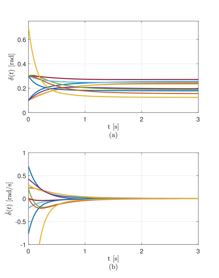
Figure 1: System responses: (a) phase angles; (b) frequency deviations

Appendix A Proof of Theorem 1

We first note a property of the Jacobian associated with (2) which follows from Proposition 2 in Appendix C. In particular, let system (2) be written as $\dot{\delta}_{i}=-k_{pi}H_{i}(\delta)$  $\forall i\in\,\mathcal{V}$, where

$$H_{i}(\delta):=\varpi_{i}+{\sum}_{j\in\mathcal{N}_{i}}(b_{ij}\sin(\delta_{ij})-a_{ij}\cos(\delta_{ij})).$$ (5)

Let the Jacobian $\tilde{\mathcal{L}}(\delta^{*})$ of the matrix of $\begin{bmatrix}H_{1}(\delta)&\cdots&H_{N}(\delta)\end{bmatrix}^{T}$ be defined as follows

$$\small\tilde{\mathcal{L}}{(\delta^{*})}=\begin{bmatrix}\small\tilde{\mathcal{L}}_{11}{(\delta^{*})}&\ldots&\tilde{\mathcal{L}}_{1N}{(\delta^{*})}\\ \vdots&\ddots&\vdots\\ \tilde{\mathcal{L}}_{N1}{(\delta^{*})}&\ldots&\tilde{\mathcal{L}}_{NN}{(\delta^{*})}\end{bmatrix}\vspace{-0.125cm}$$ (6)

where $\tilde{\mathcal{L}}_{ij}{(\delta^{*})}=\dfrac{\partial H_{i}(\delta)}{\partial\delta_{j}}\bigg{|}_{\delta=\delta^{*}}$, and $\delta^{*}\in\mathbb{T}^{n}$ is a fixed point. In Proposition 2 we show that $\tilde{\mathcal{L}}(\delta^{*})$ is a non-symmetric Laplacian matrix if the condition on the equilibrium point in Theorem 1 is satisfied. Note that by Laplacian matrix we mean that $\tilde{\mathcal{L}}_{ii}{\color[rgb]{0,0,0}(\delta^{*})}+{\sum}_{j\in\mathcal{N}_{i}}\tilde{\mathcal{L}}_{ij}{\color[rgb]{0,0,0}(\delta^{*})}=0,\,\forall i\in\mathcal{V}$ and $\tilde{\mathcal{L}}_{ii}{\color[rgb]{0,0,0}(\delta^{*})}>0,\tilde{\mathcal{L}}_{ij}{\color[rgb]{0,0,0}(\delta^{*})}<0,\,\forall j\in\mathcal{N}_{i}$.

We now proceed to prove Theorem 1. We apply centre manifold theory as described in [12, Chapter $8$], and we invoke arguments similar to those in [13, Theorem $18.1.3$] and [14, Theorem IV.$3$]. Let $\delta^{*}$ be a point generating the manifold $\mathcal{Y}_{\delta^{*}}$ in (3), and we denote by $\tilde{\delta}=\delta-\delta^{*}$ any deviation from $\delta^{*}$. We rewrite (2) as a shifted function as follows,

$${\color[rgb]{0,0,0}\dot{\tilde{\delta}}}=f(\tilde{\delta}+\delta^{*})-f(\delta^{*})\vspace{-0.125cm}$$ (7)

where $f(\tilde{\delta}+\delta^{*}):=\text{col}({\color[rgb]{0,0,0}-k_{pi}\tilde{H}_{i}(\tilde{\delta}+\delta^{*})})\in\mathbb{R}^{N}$, $f(\delta^{*}):=\text{col}({\color[rgb]{0,0,0}-k_{pi}\tilde{H}_{i}(\delta^{*})})\in\mathbb{R}^{N}$, and

$$\begin{split}\tilde{H}_{i}(\tilde{\delta}+\delta^{*})&={\sum}_{j\in\mathcal{N}_{i}}(b_{ij}\sin(\tilde{\delta}_{ij}+\delta^{*}_{ij})-a_{ij}\cos(\tilde{\delta}_{ij}+\delta^{*}_{ij})),\\ \tilde{H}_{i}(\delta^{*})&={\sum}_{j\in\mathcal{N}_{i}}(b_{ij}\sin(\delta^{*}_{ij})-a_{ij}\cos(\delta^{*}_{ij})).\vspace{-0.125cm}\end{split}$$ (8)

Model (7) is then rewritten as

$$\dot{\tilde{\delta}}=-k_{p}\tilde{\mathcal{L}}{(\delta^{*})}\tilde{\delta}+\underbrace{f(\tilde{\delta}+\delta^{*})-f(\delta^{*})+k_{p}\tilde{\mathcal{L}}{(\delta^{*})}\tilde{\delta}}_{\tilde{f}(\tilde{\delta})}\vspace{-0.125cm}$$ (9)

where $\tilde{f}(0)=0,\frac{\partial\tilde{f}}{\partial\tilde{\delta}}(0)=0$. As noted above, by Proposition 2 $\tilde{\mathcal{L}}{(\delta^{*})}$ is a Laplacian matrix, and let $k_{p}=\text{diag}(k_{pi})\in\mathbb{R}_{>0}^{N\times N}$. Noting that $k_{p}$ is diagonal with positive entries, the product $k_{p}\tilde{\mathcal{L}}{(\delta^{*})}$ has only one zero eigenvalue and all others are positive. Hence there exists a transformation matrix ${\color[rgb]{0,0,0}{\mathcal{T}}}\in\mathbb{R}^{N\times N}$ which is the eigenbasis of $k_{p}\tilde{\mathcal{L}}{(\delta^{*})}$ such that $-{\color[rgb]{0,0,0}{\mathcal{T}}}k_{p}\tilde{\mathcal{L}}{(\delta^{*})}\mathcal{T}^{-1}=\begin{bmatrix}A_{1}&0\\ 0&A_{2}\end{bmatrix}$, with $A_{1}=0$ being the single zero eigenvalue and the second block diagonal matrix $A_{2}\in\mathbb{R}^{(N-1)\times(N-1)}$ contains all the remaining negative eigenvalues (i.e. $A_{2}$ is Hurwitz). Using the coordinate transformation $[\tilde{y}~{}\tilde{z}]^{\top}={\color[rgb]{0,0,0}{\mathcal{T}}}\tilde{\delta}$, and noting that $[y~{}z]^{\top}={\color[rgb]{0,0,0}{\mathcal{T}}}\delta$, $[y^{*}~{}z^{*}]^{\top}={\color[rgb]{0,0,0}{\mathcal{T}}}\delta^{*}$, $\tilde{y}=y-y^{*},\tilde{z}=z-z^{*}$, the normal form of (9) is obtained as

$$\small\begin{split}&\begin{bmatrix}\dot{\tilde{y}}\\ \dot{\tilde{z}}\end{bmatrix}=-\mathcal{T}k_{p}\tilde{\mathcal{L}}{\left(\mathcal{T}^{-1}\begin{bmatrix}y^{*}\\ z^{*}\end{bmatrix}\right)}\mathcal{T}^{-1}\begin{bmatrix}\tilde{y}\\ \tilde{z}\end{bmatrix}+\mathcal{T}S(\tilde{y},\tilde{z})\\ \end{split}$$ (10)

where

$$\small\begin{split}S(\tilde{y},\tilde{z}):=&f\left(\mathcal{T}^{-1}\begin{bmatrix}\tilde{y}+y^{*}\\ \tilde{z}+z^{*}\end{bmatrix}\right)-f\left(\mathcal{T}^{-1}\begin{bmatrix}y^{*}\\ z^{*}\end{bmatrix}\right)\\ &+k_{p}\tilde{\mathcal{L}}{\left(\mathcal{T}^{-1}\begin{bmatrix}y^{*}\\ z^{*}\end{bmatrix}\right)}\mathcal{T}^{-1}\begin{bmatrix}\tilde{y}\\ \tilde{z}\end{bmatrix},\vspace{-0.125cm}\end{split}$$ (11)

which is compactly expressed as

$$\dot{\tilde{y}} =S_{1}(\tilde{y},\tilde{z})\vspace{-0.125cm}$$ (12a)

$$\dot{\tilde{z}} =A_{2}\tilde{z}+S_{2}(\tilde{y},\tilde{z})$$ (12b)

where similarly to $\tilde{f}$ we must have $S_{i}(0,0)=0,\frac{\partial S_{i}}{\partial\tilde{y}}(0,0)=0,\frac{\partial S_{i}}{\partial\tilde{z}}(0,0)=0,\,\text{for}\,\,i=1,2$. Since $A_{1}=0$ and $A_{2}$ is Hurwitz, then by [12, Theorem $8.1$] there exists a sufficiently small constant $\eta>0$ and a continuously differentiable function $\chi(\tilde{y})$, defined for all $\|\tilde{y}\|<\eta$, such that the invariant manifold $\tilde{z}=\chi(\tilde{y})$ for (12) is a centre manifold $W^{c}$ for (12), that is,

$$\begin{split}W^{c}=&\left\{(\tilde{y},\tilde{z})~{}\left|~{}\begin{matrix}\tilde{z}=\chi(\tilde{y}),\|\tilde{y}\|<\eta~{},\\ \chi(0)=0,\frac{\partial\chi}{\partial\tilde{y}}(0)=0\end{matrix}\right.\right\}.\vspace{-0.125cm}\end{split}$$ (13)

The reduced system restricted to the centre manifold $W^{c}$ is then given by [13, Theorem $18.1.2$]

$$\dot{\tilde{y}}=S_{1}(\tilde{y},\chi(\tilde{y})).\vspace{-0.125cm}$$ (14)

We now show that

$$W^{c}=\left\{(\tilde{y},\tilde{z})\left|\begin{matrix}&\tilde{y}=y-y^{*},\tilde{z}=z-z^{*},\\ &[y~{}z]^{\top}={\color[rgb]{0,0,0}{\mathcal{T}}}\delta,\,[y^{*}~{}z^{*}]^{\top}=\mathcal{T}\delta^{*},\delta\in\mathcal{Y}_{\delta^{*}}\end{matrix}\right.\right\}$$ (15)

is a centre manifold for (12). To show this, note that (13) implies that $W^{c}$ is tangential to the $\tilde{y}$-axis in the neighbourhood of $\tilde{y}=0$. Hence we show that $W^{c}$ in (15) has these properties. First, $W^{c}$ in (15) is invariant because it contains the steady states of (12), which follows from the fact that $\dot{\tilde{\delta}}=\mathbf{0}_{N}$ since $\delta\in\mathcal{Y}_{\delta^{*}}$. Second, $W^{c}$ in (15) is tangential to the $\tilde{y}$-axis at $\tilde{y}=0$. To see this, for sufficiently small neighbourhood of the origin we want to satisfy $S(0,0)=0$ and $\frac{\partial S}{\partial\tilde{y}}(0,0)=0$. The condition $S(0,0)=0$ trivially holds from (11). Using (11), to ensure that $\frac{\partial S}{\partial\tilde{y}}(0,0)=0$, the Jacobian of $f\left(\mathcal{T}^{-1}\begin{bmatrix}\tilde{y}+y^{*}\\ \tilde{z}+z^{*}\end{bmatrix}\right)-f\left({\color[rgb]{0,0,0}{\mathcal{T}}}^{-1}\begin{bmatrix}y^{*}\\ z^{*}\end{bmatrix}\right)=:\hat{S}(\tilde{y},\tilde{z})$ at $(\tilde{y},\tilde{z})=(0,0)$ defined by

$$\small\begin{split}\frac{\partial\hat{S}(\tilde{y},\tilde{z})}{\partial(\tilde{y},\tilde{z})}\bigg{|}_{(0,0)}&=\left.\begin{bmatrix}\frac{\partial\hat{S}_{1}(\tilde{y},\tilde{z})}{\partial\tilde{y}}&\frac{\partial\hat{S}_{1}(\tilde{y},\tilde{z})}{\partial\tilde{z}}\\ \vdots&\vdots\\ \frac{\partial\hat{S}_{N}(\tilde{y},\tilde{z})}{\partial\tilde{y}}&\frac{\partial\hat{S}_{N}(\tilde{y},\tilde{z})}{\partial\tilde{z}}\end{bmatrix}\right|_{(0,0)}\end{split}\vspace{-0.125cm}$$

must be equal to $-k_{p}\tilde{\mathcal{L}}{\left(\mathcal{T}^{-1}\begin{bmatrix}y^{*}\\ z^{*}\end{bmatrix}\right)}{\color[rgb]{0,0,0}{\mathcal{T}}}^{-1}$. We note that the columns of the right eigenvector $\mathcal{T}^{-1}$ are given by $\mathcal{T}^{-1}=[\text{span}(\mathbf{1}_{N}),v_{2},\ldots,v_{N}]$ where $v_{i}\in\mathbb{R}^{n}$, $i=2,...,N$ are the column eigenvectors. Since $\tilde{\mathcal{L}}{\left(\mathcal{T}^{-1}\begin{bmatrix}y^{*}\\ z^{*}\end{bmatrix}\right)}\text{span}(\mathbf{1}_{N})=\mathbf{0}_{N}$, then $-k_{p}\tilde{\mathcal{L}}{\left(\mathcal{T}^{-1}\begin{bmatrix}y^{*}\\ z^{*}\end{bmatrix}\right)}{\color[rgb]{0,0,0}{\mathcal{T}}}^{-1}$ has a zero first column. This means that the Jacobian entry corresponding to the $y$-component, i.e. $\left.\begin{bmatrix}\frac{\partial\hat{S}_{1}(\tilde{y},\tilde{z})}{\partial\tilde{y}}\ldots\frac{\partial\hat{S}_{N}(\tilde{y},\tilde{z})}{\partial\tilde{y}}\end{bmatrix}^{\top}\right|_{(0,0)}=\mathbf{0}_{N}$, which shows that $W^{c}$ is tangent to the $\tilde{y}$-axis at the origin $(\tilde{y},\tilde{z})=(0,0)$. Therefore, for sufficiently small neighbourhood of the origin there exists a function $\tilde{z}=\chi(\tilde{y})$ that satisfies the properties in (13), and $W^{c}$ is a centre manifold. Hence the solutions of (14) in a sufficiently small neighbourhood of the origin are in $W^{c}$ [13, Theorem $18.1.2$]. Since $W^{c}$ is composed of equilibrium points we have $\dot{\tilde{y}}=0$, thus the reduced system (14) becomes $S_{1}(\tilde{y},\chi(\tilde{y}))=0$. This implies that $\tilde{y}_{\chi}(t)=\tilde{y}_{\chi}(0)\,\forall t$, where $\tilde{y}_{\chi}(t)$ is the solution of (14), hence the origin is stable in (14). By applying [13, Theorem $18.1.3$], the origin in (14) being stable implies that $\tilde{y}(t)=\tilde{y}_{\chi}(t)+w_{1}(t)$, $\tilde{z}(t)=\chi(\tilde{y}_{\chi}(t))+w_{2}(t)$ for some solution $\tilde{y}_{\chi}(t)$ in the centre manifold $W^{c}$, and some $w_{i}(t)$ with $\|w_{i}(t)\|<k_{i}e^{-{\color[rgb]{0,0,0}\rho_{i}}t},\,i=1,2,$ and $k_{i},{\color[rgb]{0,0,0}\rho_{i}}>0$. Consequently, $\lim_{t\to\infty}(\tilde{y}(t),\tilde{z}(t))=(\tilde{y}_{\chi}(0),\chi(\tilde{y}_{\chi}(0))){\color[rgb]{0,0,0}\in W^{c}}$ and $\lim_{t\to\infty}\tilde{\delta}(t)={\color[rgb]{0,0,0}{\mathcal{T}}}^{-1}{\color[rgb]{0,0,0}[\tilde{y}_{\chi}(0)~{}~{}\chi(\tilde{y}_{\chi}(0))]^{\top}}$.

Therefore all solutions $\delta$ starting in a sufficiently small neighbourhood of $\delta^{*}$ satisfy $\lim_{t\to\infty}\|\delta(t)-\delta^{\dagger}\|\to 0$ for some $\delta^{\dagger}\in\mathcal{Y}_{\delta^{*}}$. The same also holds for solutions starting in a sufficiently small neighbourhood of any point in $\mathcal{Y}_{\delta^{*}}$, which follows from the same arguments as the ones that have been used for solutions with initial conditions in a neighbourhood of $\delta^{\ast}$. Therefore all solutions $\delta$ starting in a sufficiently small neighbourhood $\Xi$ of $\mathcal{Y}_{\delta^{*}}$ satisfy $\lim_{t\to\infty}\|\delta(t)-\delta^{\dagger}\|\to 0$ for some $\delta^{\dagger}\in\mathcal{Y}_{\delta^{*}}$.

From the boundedness of trajectories starting in $\Xi$, which can be chosen to be compact, we can also deduce the stability of $\mathcal{Y}_{\delta^{*}}$. This hence also implies its asymptotic stability using the convergence property mentioned in the previous paragraph.   $\hfill\blacksquare$

Appendix B Proof of Proposition 1

Since $\sin(\cdot)$ and $\cos(\cdot)$ are real analytic, the right-hand side of (2) is real analytic. For $f_{{\color[rgb]{0,0,0}i}}:\mathcal{C}(\gamma)\to\mathbb{R}$, let the right-hand side of (2) be $f_{{\color[rgb]{0,0,0}i}}(\delta)$. Then the right-hand side of (2) is injective in the domain $\mathcal{C}(\gamma),\gamma\in[0,\pi/2-\psi_{\max})$, that is, $f_{{\color[rgb]{0,0,0}i}}({\color[rgb]{0,0,0}\kappa}^{*}_{1})=f_{{\color[rgb]{0,0,0}i}}({\color[rgb]{0,0,0}\kappa}^{*}_{2})$ if and only if ${\color[rgb]{0,0,0}\kappa}^{*}_{1}={\color[rgb]{0,0,0}\kappa}^{*}_{2}$. Thus, $f_{{\color[rgb]{0,0,0}i}}({\color[rgb]{0,0,0}\delta})$ is a one-to-one function for ${\color[rgb]{0,0,0}\delta}^{*}\in\mathcal{C}(\gamma),\gamma\in[0,\pi/2-\psi_{\max})$ and the uniqueness of the angle differences in $\mathcal{C}{(\gamma)}$ follows. $\hfill\blacksquare$

Appendix C Proposition 2 and its proof

Proposition 2 (System expanded Laplacian matrix)

Consider system (2) together with (6). For a fixed point $\delta^{*}\in\mathbb{T}^{n}$, the Jacobian $\tilde{\mathcal{L}}{(\delta^{*})}$ in (6) is given by

$$\tilde{\mathcal{L}}{(\delta^{*})}=\mathcal{B}\text{diag}\left(\sqrt{a^{2}_{ij}+b^{2}_{ij}}\,\cos(\delta^{*}_{ij}-\psi_{ij})\right)\mathcal{B}^{\top}.\vspace{-0.125cm}$$ (16)

which can be rewritten as

$$\tilde{\mathcal{L}}{(\delta^{*})}=\mathcal{B}\text{diag}(b_{ij}\cos(\delta^{*}_{ij}))\mathcal{B}^{\top}+\mathbf{\hat{B}}\text{diag}(a_{ij}\sin(\delta^{*}_{ij}))\mathcal{B}^{\top}\vspace{-0.125cm}$$ (17)

Moreover, if $\delta^{\ast}$ is an equilibrium point that satisfies $\delta^{*}\in\mathcal{C}(\gamma)$ for some $\gamma\in[0,\pi/2-\psi_{\max})$ with $\psi_{\max}=\max_{(i,j)\in\mathcal{E}}\arctan(G_{ij}/B_{ij})$, then $\tilde{\mathcal{L}}{(\delta^{*})}$ is a non-symmetric Laplacian matrix.

Proof: The proof makes use of Lemma 1 in Appendix D. Lemma 1 shows that (2) is equivalent to

$$\dot{\delta}_{i}=k_{pi}\varpi_{i}-k_{pi}\sum_{j\in\mathcal{N}_{i}}\sqrt{a^{2}_{ij}+b^{2}_{ij}}\,\sin(\delta_{ij}-\psi_{ij}),\hskip 5.69054pt\forall i\in\mathcal{V}\vspace{-0.125cm}$$ (18)

where $\psi_{ij}=\arctan(a_{ij}/b_{ij})=\arctan(G_{ij}/B_{ij})$.

We now write (2), (18) as $\dot{\delta}_{i}=-k_{pi}H_{i}(\delta)$ as in (5) where

$$H_{i}(\delta) :=\varpi_{i}+{\sum}_{j\in\mathcal{N}_{i}}(b_{ij}\sin(\delta_{ij})-a_{ij}\cos(\delta_{ij})),$$ (19)

$$=\varpi_{i}+{\sum}_{j\in\mathcal{N}_{i}}\sqrt{a^{2}_{ij}+b^{2}_{ij}}\,\sin(\delta_{ij}-\psi_{ij}).\vspace{-0.125cm}$$ (20)

Considering (19), we have the diagonal and off-diagonal entries of $\tilde{\mathcal{L}}{(\delta^{*})}$ as

$$\begin{split}&\tilde{\mathcal{L}}_{ii}{(\delta^{*})}={\sum}_{j\in\mathcal{N}_{i}}b_{ij}\cos(\delta^{*}_{ij})+{\sum}_{j\in\mathcal{N}_{i}}a_{ij}\sin(\delta^{*}_{ij})\vspace{-0.125cm}\\ &\tilde{\mathcal{L}}_{ij}{(\delta^{*})}=-b_{ij}\cos(\delta^{*}_{ij})-a_{ij}\sin(\delta^{*}_{ij})~{}~{}~{}~{}~{}~{}~{}~{}j\in\mathcal{N}_{i}.\end{split}\vspace{-0.125cm}$$ (21)

Similarly, we obtain by considering (20)

$$\begin{split}&\tilde{\mathcal{L}}_{ii}{(\delta^{*})}={\sum}_{j\in\mathcal{N}_{i}}\sqrt{a^{2}_{ij}+b^{2}_{ij}}\,\cos(\delta^{*}_{ij}-\psi_{ij})\\ &\tilde{\mathcal{L}}_{ij}{(\delta^{*})}=-\sqrt{a^{2}_{ij}+b^{2}_{ij}}\,\cos(\delta^{*}_{ij}-\psi_{ij})~{}~{}~{}~{}~{}~{}j\in\mathcal{N}_{i}.\end{split}\vspace{-0.125cm}$$ (22)

Noting that $a_{ji}=a_{ij}$, $b_{ji}=b_{ij}$, $\cos(\delta^{*}_{ji})=\cos(\delta^{*}_{ij})$, $\sin(\delta^{*}_{ji})=-\sin(\delta^{*}_{ij})$, using (21) for all the entries of (6) gives the form (17). Likewise, using (22) for all the entries of (6) and separating the $\cos(\cdot)$ and $\sin(\cdot)$ terms gives the form (16). This completes the first part.

Note that $\tilde{\mathcal{L}}_{ii}{\color[rgb]{0,0,0}(\delta^{*})}+{\sum}_{j\in\mathcal{N}_{i}}\tilde{\mathcal{L}}_{ij}{\color[rgb]{0,0,0}(\delta^{*})}=0,\,\forall i\in\mathcal{V}$ which shows that $\tilde{\mathcal{L}}{\color[rgb]{0,0,0}(\delta^{*})}\mathbf{1}_{N}=\mathbf{0}_{N}$. Consider now $\delta^{*}\in\mathcal{C}(\gamma)$, $\gamma\in[0,\pi/2-\psi_{\max})$; then we have $\tilde{\mathcal{L}}_{ii}{\color[rgb]{0,0,0}(\delta^{*})}>0,\,\forall i\in\mathcal{V}$ and $\tilde{\mathcal{L}}_{ij}{\color[rgb]{0,0,0}(\delta^{*})}<0,\,\forall j\in\mathcal{N}_{i}$. Furthermore, we have that $\tilde{\mathcal{L}}_{ii}{\color[rgb]{0,0,0}(\delta^{*})}=-{\sum}_{j\in\mathcal{N}_{i}}\tilde{\mathcal{L}}_{ij}{\color[rgb]{0,0,0}(\delta^{*})}$ hence $\tilde{\mathcal{L}}{\color[rgb]{0,0,0}(\delta^{*})}$ is a Laplacian. The fact that $\tilde{\mathcal{L}}{(\delta^{*})}^{\top}\neq\tilde{\mathcal{L}}{(\delta^{*})}$ since $\hat{\mathbf{B}}^{\top}\neq\mathcal{B}^{\top}$ shows that $\tilde{\mathcal{L}}{(\delta^{*})}$ is a non-symmetric Laplacian matrix.

Appendix D Lemma 1 and its proof

Lemma 1 (Sine representation)

System (2) has the following equivalent representation

$$\dot{\delta}_{i}=k_{pi}\varpi_{i}-k_{pi}\sum_{j\in\mathcal{N}_{i}}\sqrt{a^{2}_{ij}+b^{2}_{ij}}\,\sin(\delta_{ij}-\psi_{ij}),\hskip 5.69054pt\forall i\in\mathcal{V}$$

where $\psi_{ij}=\arctan(a_{ij}/b_{ij})=\arctan(G_{ij}/B_{ij})$.

Proof: Considering (2), we rewrite $P_{ij}{\color[rgb]{0,0,0}:=}b_{ij}\sin(\delta_{ij})-a_{ij}\cos(\delta_{ij})$ as ${\scriptsize P_{ij}=\left(\frac{b_{ij}\sin(\delta_{ij})}{\sqrt{a^{2}_{ij}+b^{2}_{ij}}}-\frac{a_{ij}\cos(\delta_{ij})}{\sqrt{a^{2}_{ij}+b^{2}_{ij}}}\right)\sqrt{a^{2}_{ij}+b^{2}_{ij}}}$. Let $\scriptsize{\cos(\psi_{ij})=\frac{b_{ij}}{\sqrt{a^{2}_{ij}+b^{2}_{ij}}}}$, $\scriptsize{\sin(\psi_{ij})}=\frac{a_{ij}}{\sqrt{b^{2}_{ij}+b^{2}_{ij}}}$, thus $\scriptsize{\psi_{ij}=\arctan(\frac{\sin(\psi_{ij})}{\cos(\psi_{ij})})}=\arctan(G_{ij}/B_{ij})$. Then ${\scriptsize P_{ij}=\sqrt{a^{2}_{ij}+b^{2}_{ij}}\,\left(\cos(\psi_{ij})\sin(\delta_{ij})-\sin(\psi_{ij})\cos(\delta_{ij})\right)}$ or ${\scriptsize P_{ij}=}$${\sqrt{a^{2}_{ij}+b^{2}_{ij}}\,\sin(\delta_{ij}-\psi_{ij})}$ which transforms (2) into $\dot{\delta}_{i}$ of Lemma 1.

References

- [1] Y. Kuramoto, “Chemical oscillations, waves and turbulence. mineola,” 2003.
- [2] F. Dorfler and F. Bullo, “Synchronization and transient stability in power networks and nonuniform kuramoto oscillators,” SIAM Journal on Control and Optimization, vol. 50, no. 3, pp. 1616–1642, 2012.
- [3] J. W. Simpson-Porco, F. Dörfler, and F. Bullo, “Synchronization and power sharing for droop-controlled inverters in islanded microgrids,” Automatica, vol. 49, no. 9, pp. 2603–2611, 2013.
- [4] J. Schiffer, D. Goldin, J. Raisch, and T. Sezi, “Synchronization of droop-controlled microgrids with distributed rotational and electronic generation,” in 52nd IEEE Conference on Decision and Control. IEEE, 2013, pp. 2334–2339.
- [5] R. Olfati-Saber, J. A. Fax, and R. M. Murray, “Consensus and cooperation in networked multi-agent systems,” Proceedings of the IEEE, vol. 95, no. 1, pp. 215–233, 2007.
- [6] Z. Lin, B. Francis, and M. Maggiore, “State agreement for continuous-time coupled nonlinear systems,” SIAM Journal on Control and Optimization, vol. 46, no. 1, pp. 288–307, 2007.
- [7] A. Jadbabaie, N. Motee, and M. Barahona, “On the stability of the kuramoto model of coupled nonlinear oscillators,” in Proceedings of the 2004 American Control Conference, vol. 5. IEEE, 2004, pp. 4296–4301.
- [8] N. Chopra and M. W. Spong, “On exponential synchronization of kuramoto oscillators,” IEEE transactions on Automatic Control, vol. 54, no. 2, pp. 353–357, 2009.
- [9] F. Dörfler and F. Bullo, “On the critical coupling for kuramoto oscillators,” SIAM Journal on Applied Dynamical Systems, vol. 10, no. 3, pp. 1070–1099, 2011.
- [10] ——, “Exploring synchronization in complex oscillator networks,” in 2012 IEEE 51st IEEE Conference on Decision and Control (CDC). IEEE, 2012, pp. 7157–7170.
- [11] S.-Y. Ha, Y. Kim, and Z. Li, “Large-time dynamics of kuramoto oscillators under the effects of inertia and frustration,” SIAM Journal on Applied Dynamical Systems, vol. 13, no. 1, pp. 466–492, 2014.
- [12] H. K. Khalil, Nonlinear Systems, 3rd ed. Pearson New York, 2015.
- [13] S. Wiggins and M. Golubitsky, Introduction to applied nonlinear dynamical systems and chaos. Springer, 2003, vol. 2, no. 3.
- [14] T. Jouini and Z. Sun, “Frequency synchronization of a high-order multi-converter system,” IEEE Transactions on Control of Network Systems, 2021.
- [15] P. Kundur, N. J. Balu, and M. G. Lauby, Power system stability and control. McGraw-hill New York, 1994, vol. 7.
- [16] F. Dorfler and F. Bullo, “Kron reduction of graphs with applications to electrical networks,” IEEE Transactions on Circuits and Systems I: Regular Papers, vol. 60, no. 1, pp. 150–163, 2012.
- [17] J. Schiffer, R. Ortega, A. Astolfi, J. Raisch, and T. Sezi, “Conditions for stability of droop-controlled inverter-based microgrids,” Automatica, vol. 50, no. 10, pp. 2457–2469, 2014.
- [18] J. Schiffer, D. Zonetti, R. Ortega, A. M. Stanković, T. Sezi, and J. Raisch, “A survey on modeling of microgrids—from fundamental physics to phasors and voltage sources,” Automatica, vol. 74, pp. 135 – 150, 2016.
- [19] F. Dörfler, M. Chertkov, and F. Bullo, “Synchronization in complex oscillator networks and smart grids,” Proceedings of the National Academy of Sciences, vol. 110, no. 6, pp. 2005–2010, 2013.
- [20] N. Pogaku, M. Prodanovic, and T. C. Green, “Modeling, analysis and testing of autonomous operation of an inverter-based microgrid,” IEEE Transactions on Power Electronics, vol. 22, no. 2, pp. 613–625, 2007.
- [21] Y. Ojo, J. Watson, and I. Lestas, “An improved control scheme for grid-forming inverters,” in 2019 IEEE PES Innovative Smart Grid Technologies Europe (ISGT-Europe). IEEE, 2019, pp. 1–5.
- [22] Y. Ojo, J. Watson, K. Laib, and I. Lestas, “A decentralized frequency and voltage control scheme for grid-forming inverters,” 2021 IEEE PES Innovative Smart Grid Technologies Europe (ISGT Europe), pp. 1–5, 2021.
- [23] J. M. Guerrero, L. G. de Vicuna, J. Matas, M. Castilla, and J. Miret, “Output impedance design of parallel-connected ups inverters with wireless load-sharing control,” IEEE Transactions on Industrial Electronics, vol. 52, no. 4, pp. 1126–1135, 2005.
- [24] J. He, Y. W. Li, J. M. Guerrero, F. Blaabjerg, and J. C. Vasquez, “An islanding microgrid power sharing approach using enhanced virtual impedance control scheme,” IEEE Transactions on Power Electronics, vol. 28, no. 11, pp. 5272–5282, 2013.
- [25] Y. Sun, X. Hou, J. Yang, H. Han, M. Su, and J. M. Guerrero, “New perspectives on droop control in ac microgrid,” IEEE Transactions on Industrial Electronics, vol. 64, no. 7, pp. 5741–5745, 2017.