Optimal Transport for Unsupervised Hallucination Detection
in Neural Machine Translation

Abstract

Neural machine translation (NMT) has become the de-facto standard in real-world machine translation applications. However, NMT models can unpredictably produce severely pathological translations, known as hallucinations, that seriously undermine user trust. It becomes thus crucial to implement effective preventive strategies to guarantee their proper functioning. In this paper, we address the problem of hallucination detection in NMT by following a simple intuition: as hallucinations are detached from the source content, they exhibit cross-attention patterns that are statistically different from those of good quality translations. We frame this problem with an optimal transport formulation and propose a fully unsupervised, plug-in detector that can be used with any attention-based NMT model. Experimental results show that our detector not only outperforms all previous model-based detectors, but is also competitive with detectors that employ external models trained on millions of samples for related tasks such as quality estimation and cross-lingual sentence similarity.

1 Introduction

Neural machine translation (NMT) has achieved tremendous success (Vaswani et al., 2017; Kocmi et al., 2022), becoming the mainstream method in real-world applications and production systems for automatic translation. Although these models are becoming evermore accurate, especially in high-resource settings, they may unpredictably produce hallucinations. These are severely pathological translations that are detached from the source sequence content (Lee et al., 2018; Müller et al., 2020; Raunak et al., 2021; Guerreiro et al., 2023). Crucially, these errors have the potential to seriously harm user trust in hard-to-predict ways Perez et al. (2022), hence the evergrowing need to develop security mechanisms. One appealing strategy to address this issue is to develop effective on-the-fly detection systems.

In this work, we focus on leveraging the cross-attention mechanism to develop a novel hallucination detector. This mechanism is responsible for selecting and combining the information contained in the source sequence that is relevant to retain during translation. Therefore, as hallucinations are translations whose content is detached from the source sequence, it is no surprise that connections between anomalous attention patterns and hallucinations have been drawn before in the literature (Berard et al., 2019; Raunak et al., 2021; Ferrando et al., 2022). These patterns usually exhibit scattered source attention mass across the different tokens in the translation (e.g. most source attention mass is concentrated on a few irrelevant tokens such as punctuation and the end-of-sequence token). Inspired by such observations, previous work has designed ad-hoc heuristics to detect hallucinations that specifically target the anomalous maps. While such heuristics can be used to detect hallucinations to a satisfactory extent (Guerreiro et al., 2023), we argue that a more theoretically-founded way of using anomalous attention information for hallucination detection is lacking in the literature.

Rather than aiming to find particular patterns, we go back to the main definition of hallucinations and draw the following hypothesis: as hallucinations—contrary to good translations—are not supported by the source content, they may exhibit cross-attention patterns that are statistically different from those found in good quality translations. Based on this hypothesis, we approach the problem of hallucination detection as a problem of anomaly detection with an optimal transport (OT) formulation (Kantorovich, 2006; Peyré et al., 2019). Namely, we aim to find translations with source attention mass distributions that are highly distant from those of good translations. Intuitively, the more distant a translation’s attention patterns are from those of good translations, the more anomalous it is in light of that distribution.

Our key contributions are:

• We propose an OT-inspired fully unsupervised hallucination detector that can be plugged into any attention-based NMT model;

• We find that the idea that attention maps for hallucinations are anomalous in light of a reference data distribution makes for an effective hallucination detector;

• We show that our detector not only outperforms all previous model-based detectors, but is also competitive with external detectors that employ auxiliary models that have been trained on millions of samples.

2 Background

2.1 Cross-attention in NMT models

A NMT model $\mathcal{M}$ defines a probability distribution $p_{\bm{\theta}}(\bm{y}|\bm{x})$ over an output space of hypotheses $\mathcal{Y}$ conditioned on a source sequence $\bm{x}$ contained in an input space $\mathcal{X}$. In this work, we focus on models parameterized by an encoder-decoder transformer model (Vaswani et al., 2017) with a set of learned weights $\bm{\theta}$. In particular, we will look closely at the cross-attention mechanism, a core component of NMT models that has been extensively analysed in the literature (Bahdanau et al., 2014; Raganato and Tiedemann, 2018; Kobayashi et al., 2020; Ferrando and Costa-jussà, 2021). This mechanism is responsible for computing, at each generation step, a distribution over all source sentence words that informs the decoder on the relevance of each of those words to the current translation generation step. We follow previous work that has drawn connections between hallucinations and cross-attention (Berard et al., 2019; Raunak et al., 2021), and focus specifically on the last layer of the decoder module. Concretely, for a source sequence of arbitrary length $n$ and a target sequence of arbitrary length $m$, we will designate as $\bm{\Omega}\in[0,1]^{m\times n}$ the matrix of attention weights that is obtained by averaging across all the cross-attention heads of the last layer of the decoder module. Further, given the model $\mathcal{M}$ we will designate $\bm{\pi}_{\mathcal{M}}(\bm{x}):=\frac{1}{m}\left[\bm{\Omega}(\bm{x})\right]^{\top}\bm{1}\in\triangle_{n}$ as the source (attention) mass distribution computed by $\mathcal{M}$ when $\bm{x}$ is presented as input, where $\triangle_{n}=\{\bm{p}\in\mathbb{R}^{n}\,|\,\bm{p}\geq\bm{0},\,\bm{1}^{\top}\bm{p}=1\}$ is the $(n-1)$-dimensional probability simplex.

2.2 Optimal Transport Problem and Wasserstein Distance

The first-order Wasserstein distance between two arbitrary probability distributions $\bm{\mu}\in\triangle_{n}$ and $\bm{\nu}\in\triangle_{m}$ is defined as

$$W(\bm{\mu},\bm{\nu})=\inf_{\bm{\gamma}\in\Pi(\bm{\mu},\bm{\nu})}\mathbb{E}_{(u,v)\sim\bm{\gamma}}\,\left[c(u,v)\right],$$ (1)

where $c:[n]\times[m]\rightarrow\mathbb{R}_{0}^{+}$ is a cost function, and $\Pi(\bm{\mu},\bm{\nu})=\{\bm{\gamma}\in\triangle_{n\times m}:\bm{\gamma}\bm{1}=\bm{\mu};\bm{\gamma}^{\top}\bm{1}=\bm{\nu}\}$ is the set of all joint probability distributions whose marginals are $\bm{\mu}$, $\bm{\nu}$. The Wasserstein distance arises from the method of optimal transport (OT) (Kantorovich, 2006; Peyré et al., 2019): OT measures distances between distributions in a way that depends on the geometry of the sample space. Intuitively, this distance indicates how much probability mass must be transferred from $\bm{\mu}$ to $\bm{\nu}$ in order to transform $\bm{\mu}$ into $\bm{\nu}$ while minimizing the transportation cost defined by $c$.

A notable example is the Wasserstein-1 distance, $W_{1}$, also known as Earth Mover’s Distance (EMD), obtained for $c(u,v)=\|u-v\|_{1}$. The name follows from the simple intuition: if the distributions are interpreted as “two piles of mass” that can be moved around, the EMD represents the minimum amount of “work” required to transform one pile into the other, where the work is defined as the amount of mass moved multiplied by the distance it is moved.

Although OT has been explored for robustness Paty and Cuturi (2019); Staerman et al. (2021) and out-of-distribution detection Wang et al. (2021); Yan et al. (2021); Cheng et al. (2022) in computer vision, the use of OT for anomaly detection in NLP applications remains largely overlooked.

2.3 The problem of hallucinations in NMT

Hallucinations are translations that lie at the extreme end of NMT pathologies (Raunak et al., 2021). Despite being a well-known issue, research on the phenomenon is hindered by the fact that these translations are rare, especially in high-resource settings. As a result, data with hallucinations is scarce. To overcome this obstacle, many previous studies have focused on amplified settings where hallucinations are more likely to occur or are easier to detect. These include settings where (i) perturbations are induced either in the source sentence or in the target prefix (Lee et al., 2018; Müller and Sennrich, 2021; Voita et al., 2021; Ferrando et al., 2022); (ii) the training data is corrupted with noise (Raunak et al., 2021); (iii) the model is tested under domain shift (Wang and Sennrich, 2020; Müller et al., 2020); (iv) the detectors are validated on artificial hallucinations (Zhou et al., 2021). Nevertheless, these works have provided important insights towards better understanding of the phenomenon. For instance, it has been found that samples memorized by an NMT model are likely to generate hallucinations when perturbed (Raunak et al., 2021), and hallucinations are related to lower source contributions and over-reliance on the target prefix (Voita et al., 2021; Ferrando et al., 2022).

In this work, we depart from artificial settings, and focus on studying hallucinations that are naturally produced by the NMT model. To that end, we follow the taxonomy introduced in Raunak et al. (2021) and later extended and studied in Guerreiro et al. (2023). Under this taxonomy, hallucinations are translations that contain content that is detached from the source sentence. To disentangle the different types of hallucinations, they can be categorized as: largely fluent detached hallucinations or oscillatory hallucinations. The former are translations that bear little or no relation at all to the source content and may be further split according to the severity of the detachment (e.g. strong or full detachment) while the latter are inadequate translations that contain erroneous repetitions of words and phrases. We illustrate in Appendix A the categories described above through examples of hallucinated outputs.

3 On-the-fly detection of hallucinations

On-the-fly hallucination detectors are systems that can detect hallucinations without access to reference translations. These detectors are particularly relevant as they can be deployed in online applications where references are not readily available.

3.1 Categorization of hallucination detectors

Previous work on on-the-fly detection of hallucinations in NMT has primarily focused on two categories of detectors: external detectors and model-based detectors. External detectors employ auxiliary models trained for related tasks such as quality estimation (QE) and cross-lingual embedding similarity. On the other hand, model-based detectors only require access to the NMT model that generates the translations, and work by leveraging relevant internal features such as model confidence and cross-attention. These detectors are attractive due to their flexibility and low memory footprint, as they can very easily be plugged in on a vast range of NMT models without the need for additional training data or computing infrastructure. Moreover, Guerreiro et al. (2023) show that model-based detectors can be predictive of hallucinations, outperforming QE models and even performing on par with state-of-the-art reference-based metrics.

3.2 Problem Statement

We will focus specifically on model-based detectors that require obtaining internal features from a model $\mathcal{M}$. Building a hallucination detector generally consists of finding a scoring function $s_{\mathcal{M}}:\mathcal{X}\rightarrow\mathbb{R}$ and a threshold $\tau\in\mathbb{R}$ to build a binary rule $g_{\mathcal{M}}:\mathcal{X}\rightarrow\{0,1\}$. For a given test sample $\bm{x}\in\mathcal{X}$,

$$g_{\mathcal{M}}(\bm{x})=\mathbbm{1}{\{s_{\mathcal{M}}(\bm{x})>\tau\}}.$$ (2)

If $s_{\mathcal{M}}$ is an anomaly score, $g_{\mathcal{M}}(\bm{x})=0$ implies that the model $\mathcal{M}$ generates a ‘normal’ translation for the source sequence $\bm{x}$, and $g_{\mathcal{M}}(\bm{x})=1$ implies that $\mathcal{M}$ generates a ‘hallucination’ instead.

4 Unsupervised Hallucination Detection with Optimal Transport

Anomalous cross-attention maps have been connected to the hallucinatory mode in several works (Lee et al., 2018; Berard et al., 2019; Raunak et al., 2021). Our method builds on this idea and uses the Wasserstein distance to estimate the cost of transforming a translation source mass distribution into a reference distribution. Intuitively, the higher the cost of such transformation, the more distant—and hence the more anomalous— the attention of the translation is with respect to that of the reference translation.

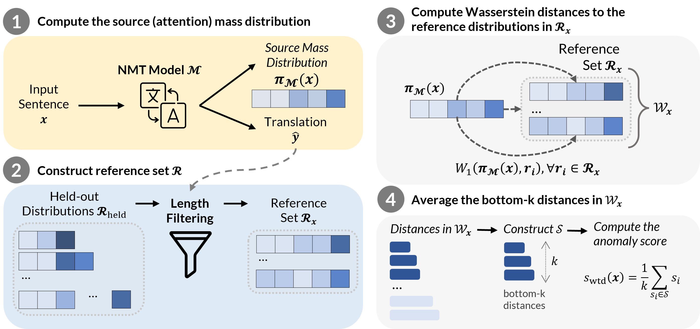
Figure 1: Procedure diagram for computation of the detection scores for the data-driven method Wass-to-Data.

4.1 Wass-to-Unif: A data independent scenario

In this scenario, we only rely on the generated translation and its source mass distribution to decide whether the translation is a hallucination or not. Concretely, for a given test sample $\bm{x}\in\mathcal{X}$:

1. We first obtain the source mass attention distribution $\bm{\pi}_{\mathcal{M}}(\bm{x})\in\triangle_{|\bm{x}|}$;

2. We then compute an anomaly score, $s_{\textsf{wtu}}(\bm{x})$, by measuring the Wasserstein distance between $\bm{\pi}_{\mathcal{M}}(\bm{x})$ and a reference distribution $\bm{u}$:

   $$\textstyle s_{\textsf{wtu}}(\bm{x})=W(\bm{\pi}_{\mathcal{M}}(\bm{x}),\bm{u}).$$ (3)

Choice of reference translation.

A natural choice for $\bm{u}$ is the uniform distribution, $\bm{u}=\frac{1}{n}\cdot\bm{1}$, where $\bm{1}$ is a vector of ones of size $n$. In the context of our problem, a uniform source mass distribution means that all source tokens are equally attended.

Choice of cost function.

We consider the 0/1 cost function, $c(i,j)=\bm{1}[i\neq j]$, as it guarantees that the cost of transporting a unit mass from any token $i$ to any token $j\neq i$ is constant. For this distance function, the problem in Equation 1 has the following closed-form solution (Villani, 2009):

$$W(\bm{\pi}_{\mathcal{M}}(\bm{x}),\bm{u})=\nicefrac{{1}}{{2}}\,\|\bm{\pi}_{\mathcal{M}}(\bm{x})-\bm{u}\|_{1}.$$ (4)

This is a well-known result in optimal transport: the Wasserstein distance under the $0/1$ cost function is equivalent to the total variation distance between the two distributions. On this metric space, the Wasserstein distance depends solely on the probability mass that is transported to transform $\bm{\pi}_{\mathcal{M}}(\bm{x})$ to $\bm{u}$. Importantly, this formulation ignores the starting locations and destinations of that probability mass as the cost of transporting a unit mass from any token $i$ to any token $j\neq i$ is constant.

Interpretation of Wass-to-Unif.  Attention maps for which the source attention mass is highly concentrated on a very sparse set of tokens (regardless of their location in the source sentence) can be very predictive of hallucinations (Berard et al., 2019; Guerreiro et al., 2023). Thus, the bigger the distance between the source mass distribution of a test sample and the uniform distribution, the more peaked the former is, and hence the closer it is to such predictive patterns.

4.2 Wass-to-Data: A data-driven scenario

In this scenario, instead of using a single reference distribution, we use a set of reference source mass distributions, $\mathcal{R}_{\bm{x}}$, obtained with the same model. By doing so, we can evaluate how anomalous a given translation is compared to a model data-driven distribution, rather than relying on an arbitrary choice of reference distribution.

First, we use a held-out dataset $\mathcal{D}_{\textrm{held}}$ that contains samples for which the model $\mathcal{M}$ generates good quality translations according to an automatic evaluation metric (in this work, we use COMET (Rei et al., 2020)). We use this dataset to construct (offline) a set of held-out source attention distributions $\mathcal{R}_{\textrm{held}}=\{\bm{\pi}_{\mathcal{M}}(\bm{x})\in\triangle_{|\bm{x}|}:\bm{x}\in\mathcal{D}_{\textrm{held}}\}$. Then, for a given test sample $\bm{x}\in\mathcal{X}$, we apply the procedure illustrated in Figure 1:

1. We generate a translation $\hat{\bm{y}}=(y_{1},\dots,y_{m})$ and obtain the source mass attention distribution $\bm{\pi}_{\mathcal{M}}(\bm{x})\in\triangle_{|\bm{x}|}$;

2. We apply a length filter to construct the sample reference set $\mathcal{R}_{\bm{x}}$, by restricting $\mathcal{R}_{\bm{x}}$ to contain source mass distributions of $\mathcal{R}_{\text{held}}$ correspondent to translations of size $[(1-\delta)m,(1+\delta)m]$ for a predefined $\delta\in]0,1[$;

3. We compute pairwise Wasserstein-1 distances between $\bm{\pi}_{\mathcal{M}}(\bm{x})$ and each element $\bm{r}_{i}$ of $\mathcal{R}_{\bm{x}}$:

   $$\mathcal{W}_{\bm{x}}=\bigl{(}W_{1}( \bm{\pi}_{\mathcal{M}}(\bm{x}),\bm{r}_{1}),\dots,$$ (5)

   $$\left.W_{1}(\bm{\pi}_{\mathcal{M}}(\bm{x}),\bm{r}_{|\mathcal{R}_{\bm{x}}|})\right).$$

4. We obtain the anomaly score $s_{\textsf{wtd}}(\bm{x})$ by averaging the bottom-$k$ distances in $\mathcal{W}_{\bm{x}}$:

   $$\textstyle s_{\textsf{wtd}}(\bm{x})=\frac{1}{k}\,\sum_{s_{i}\in\mathcal{S}}s_{i},$$ (6)

   where $\mathcal{S}$ is the set containing the $k$ smallest elements of $\mathcal{W}_{\bm{x}}$.

Interpretation of Wass-to-Data.

Hallucinations, unlike good translations, are not fully supported by the source content. Wass-to-Data evaluates how anomalous a translation is by comparing the source attention mass distribution of that translation to those of good translations. The higher the Wass-to-Data score, the more anomalous the source attention mass distribution of that translation is in comparison to those of good translations, and the more likely it is to be an hallucination.

Relation to Wass-to-Unif.

The Wasserstein-1 distance (see Section 2.2) between two distributions is equivalent to the $\ell_{1}$-norm of the difference between their cumulative distribution functions (Peyré and Cuturi, 2018). Note that this is different from the result in Equation 4, as the Wasserstein distance under $c(i,j)=\bm{1}[i\neq j]$ as the cost function is proportional to the norm of the difference between their probability mass functions. Thus, Wass-to-Unif will be more sensitive to the overall structure of the distributions (e.g. sharp probability peaks around some points), whereas Wass-to-Data will be more sensitive to the specific values of the points in the two distributions.

4.3 Wass-Combo: The best of both worlds

With this scoring function, we aim at combining Wass-to-Unif and Wass-to-Data into a single detector. To do so, we propose using a two-stage process that exploits the computational benefits of Wass-to-Unif over Wass-to-Data. Put simply, (i) we start by assessing whether a test sample is deemed a hallucination according to Wass-to-Unif, and if not (ii) we compute the Wass-to-Data score. Formally,

$$s_{\textsf{wc}}(\bm{x})=\mathbbm{1} \left[s_{\textsf{wtu}}(\bm{x})>\tau_{\textsf{wtu}}\right]\times\tilde{s}_{\textsf{wtu}}(\bm{x})$$ (7)

$$+\mathbbm{1}\left[s_{\textsf{wtu}}(\bm{x})\leq\tau_{\textsf{wtu}}\right]\times s_{\textsf{wtd}}(\bm{x})$$

for a predefined scalar threshold $\tau_{\textsf{wtu}}$. To set that threshold, we compute $\mathcal{W}_{\textsf{wtu}}=\{s_{\textsf{wtu}}(\bm{x}):\bm{x}\in\mathcal{D}_{\textrm{held}}\}$ and set $\tau_{\textsf{wtu}}=P_{K}$, i.e $\tau_{\textsf{wtu}}$ is the $K$^th percentile of $\mathcal{W}_{\textsf{wtu}}$ with $K\in\,]98,100[$ (in line with hallucinatory rates reported in (Müller et al., 2020; Wang and Sennrich, 2020; Raunak et al., 2022)).

5 Experimental Setup

5.1 Model and Data

We follow the setup in Guerreiro et al. (2023). In that work, the authors released a dataset of 3415 translations for WMT18 de-en news translation data (Bojar et al., 2018) with annotations on critical errors and hallucinations. Our analysis in the main text focuses on this dataset as it is the only available dataset that contains human annotations on hallucinations produced naturally by an NMT model (we provide full details about the dataset and the model in Appendix A). Nevertheless, in order to access the broader validity of our methods for other low and mid-resource language pairs and models, we follow a similar setup to that of Tang et al. (2022) in which quality assessments are converted to hallucination annotations. For those experiments, we use the ro-en (mid-resource) and ne-en (low-resource) translations from the MLQE-PE dataset (Fomicheva et al., 2022). In Appendix J, we present full details on the setup and report the results of these experiments. Importantly, our empirical observations are similar to those of the main text. For all our experiments, we obtain all model-based information required to build the detectors using the same models that generated the translations in consideration.

Figure 2: Histogram scores for our methods – Wass-to-Unif (left), Wass-to-Data (center) and Wass-Combo (right). We display Wass-to-Data and Wass-Combo scores on log-scale.

5.2 Baseline detectors

5.2.1 Model-based detectors

We compare our methods to the two best performing model-based methods in Guerreiro et al. (2023).

Attn-ign-SRC.

This method consists of computing the proportion of source words with a total incoming attention mass lower than a threshold $\lambda$:

$$\textstyle s_{\textsf{ais}}(\bm{x})=\frac{1}{n}\sum_{j=1}^{n}\mathbbm{1}\left[(\bm{\Omega}^{\top}(\bm{x})\bm{1})_{j}<\lambda\right].$$ (8)

This method was initially proposed in Berard et al. (2019). We follow their work and use $\lambda=0.2$.

Seq-Logprob.

We compute the length-normalised sequence log-probability of the translation:

$$\textstyle s_{\textsf{slp}}(\bm{x})=\frac{1}{m}\sum_{k=1}^{m}\log p_{\bm{\theta}}(y_{k}\mid\bm{y}_{<k},\bm{x}).$$ (9)

5.2.2 External detectors

We provide a comparison to detectors that exploit state-of-the-art models in related tasks, as it helps monitor the development of model-based detectors.

CometKiwi.

We compute sentence-level quality scores with CometKiwi (Rei et al., 2022), the winning reference-free model of the WMT22 QE shared task (Zerva et al., 2022). It has more than 565M parameters and it was trained on more than 1M human quality annotations. Importantly, this training data includes human annotations for several low-quality translations and hallucinations.

LaBSE.

We leverage LaBSE (Feng et al., 2020) to compute cross-lingual sentence representations for the source sequence and translation. We use the cosine similarity of these representations as the detection score. The model is based on the BERT (Devlin et al., 2019) architecture and was trained on more than 20 billion sentences. LaBSE makes for a good baseline, as it was optimized in a self-supervised way with a translate matching objective that is very much aligned with the task of hallucination detection: during training, LaBSE is given a source sequence and a set of translations including the true translation and multiple negative alternatives, and the model is optimized to specifically discriminate the true translation from the other negative alternatives by assigning a higher similarity score to the former.

5.3 Evaluation metrics

We report the Area Under the Receiver Operating Characteristic curve (AUROC) and the False Positive Rate at 90% True Positive Rate (FPR@90TPR) to evaluate the performance of different detectors.

5.4 Implementation Details

We use WMT18 de-en data samples from the held-out set used in Guerreiro et al. (2023), and construct $\mathcal{D}_{\text{held}}$ to contain the 250k samples with highest COMET score. To obtain Wass-to-Data scores, we set $\delta=0.1$, $|\mathcal{R}|_{\text{max}}=1000$ and $k=4$. To obtain Wass-to-Combo scores, we set $\tau_{\textsf{wtu}}=P_{99.9}$. We perform extensive ablations on the construction of $\mathcal{R}_{\text{held}}$ and on all other hyperparameters in Appendix G. We also report the computational runtime of our methods in Appendix D.

6 Results

6.1 Performance on on-the-fly detection

We start by analyzing the performance of our proposed detectors on a real world on-the-fly detection scenario. In this scenario, the detector must be able to flag hallucinations regardless of their specific type as those are unknown at the time of detection.

Detector	AUROC $\uparrow$	FPR@90TPR $\downarrow$
External Detectors
CometKiwi	86.96	53.61
LaBSE	91.72	26.91
1-3[.4pt/2pt] Model-based Detectors
Attn-ign-SRC	79.36	72.83
Seq-Logprob	83.40	59.02
Ours
Wass-to-Unif	80.37	72.22
Wass-to-Data	84.20 0.15	48.15 0.54
Wass-Combo	87.17 0.07	47.56 1.30

Table 1: Performance of all hallucination detectors. For Wass-to-Data and Wass-Combo we present the mean and standard deviation scores across five random seeds.

Wass-Combo is the best model-based detector.

Table 6.1 shows that Wass-Combo outperforms most other methods both in terms of AUROC and FPR. When compared to the previous best-performing model-based method (Seq-Logprob), Wass-Combo obtains boosts of approximately $4$ and $10$ points in AUROC and FPR, respectively. These performance boosts are further evidence that model-based features can be leveraged, in an unsupervised manner, to build effective detectors. Nevertheless, the high values of FPR suggest that there is still a significant performance margin to reduce in future research.

The notion of data proximity is helpful to detect hallucinations.

Table 6.1 shows that Wass-to-Data outperforms the previous best-performing model-based method (Seq-Logprob) in both AUROC and FPR (by more than $10\%$). This supports the idea that cross-attention patterns for hallucinations are anomalous with respect to those of good model-generated translations, and that our method can effectively measure this level of anomalousness. On the other hand, compared to Wass-to-Uni, Wass-to-Data shows a significant improvement of 30 FPR points. This highlights the effectiveness of leveraging the data-driven distribution of good translations instead of the ad-hoc uniform distribution. Nevertheless, Table 6.1 and Figure 2 show that combining both methods brings further performance improvements. This suggests that these methods may specialize in different types of hallucinations, and that combining them allows for detecting a broader range of anomalies. We will analyze this further in Section 6.2.

Our model-based method achieves comparable performance to external models.

Table 6.1 shows that Wass-Combo outperforms CometKiwi, with significant improvements on FPR. However, there still exists a gap to LaBSE, the best overall detector. This performance gap indicates that more powerful detectors can be built, paving the way for future work in model-based hallucination detection. Nevertheless, while relying on external models seems appealing, deploying and serving them in practice usually comes with additional infrastructure costs, while our detector relies on information that can be obtained when generating the translation.

Translation quality assessments are less predictive than similarity of cross-lingual sentence representations.

Table 6.1 shows that LaBSE outperforms the state-of-the-art quality estimation system CometKiwi, with vast improvements in terms of FPR. This shows that for hallucination detection, quality assessments obtained with a QE model are less predictive than the similarity between cross-lingual sentence representations. This may be explained through their training objectives (see Section 5.2.2): while CometKiwi employs a more general regression objective in which the model is trained to match human quality assessments, LaBSE is trained with a translate matching training objective that is very closely related to the task of hallucination detection.

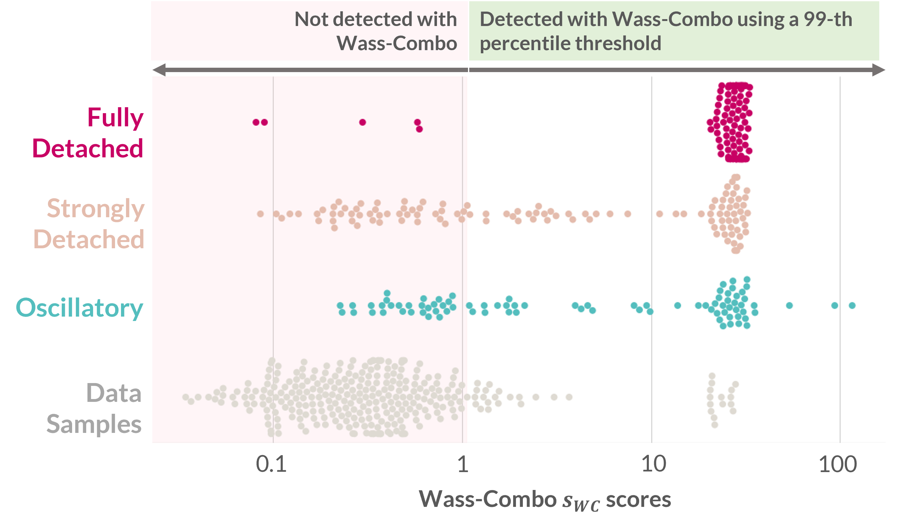
Figure 3: Distribution of Wass-Combo scores (on log-scale) for hallucinations and data samples, and performance on a fixed-threshold scenario.

Detector	Fully	Oscillatory	Strongly
	Detached		Detached
External Detectors
CometKiwi	87.75	93.04	81.78
LaBSE	98.91	84.62	89.72
1-4[.4pt/2pt]      Model-based Detectors
Attn-ign-SRC	95.76	59.53	77.42
Seq-Logprob	95.64	71.10	80.15
Ours
Wass-to-Unif	96.35	69.75	72.19
Wass-to-Data	88.24 0.29	87.80 0.10	77.60 0.18
Wass-Combo	96.57 0.10	85.74 0.10	78.89 0.15

(a) AUROC – the higher the better.

Detector	Fully	Oscillatory	Strongly
	Detached		Detached
External Detectors
CometKiwi	33.70	23.80	42.98
LaBSE	0.52	50.26	28.88
1-4[.4pt/2pt]      Model-based Detectors
Attn-ign-SRC	8.51	81.24	76.68
Seq-Logprob	4.62	72.99	65.39
Ours
Wass-to-Unif	3.27	78.78	88.32
Wass-to-Data	36.60 1.92	40.04 1.57	63.96 2.04
Wass-Combo	3.56 0.00	41.38 1.59	64.55 1.93

(b) FPR@90TPR ($\%$) – the lower the better.

(c) Performance of all hallucination detectors for each hallucination type. For Wass-to-Data and Wass-Combo, we present the mean and standard deviation across five random seeds.

6.2 Do detectors specialize in different types of hallucinations?

In this section, we present an analysis on the performance of different detectors for different types of hallucinations (see Section 2.3). We report both a quantitative analysis to understand whether a detector can distinguish a specific hallucination type from other translations (Table 6.1), and a qualitative analysis on a fixed-threshold scenario (Figure 3). This analysis is particularly relevant to better understand how different detectors specialize in different types of hallucinations. In Appendix J, we show that the trends presented in this section hold for other mid- and low-resource language pairs.

Fully detached hallucinations.

Detecting fully detached hallucinations is remarkably easy for most detectors. Interestingly, Wass-to-Unif significantly outperforms Wass-to-Data on this type of hallucination. This highlights how combining both methods can be helpful. In fact, Wass-Combo performs similarly to Wass-to-Unif, and can very easily separate most fully detached hallucinations from other translations on a fixed-threshold scenario (Figure 3). Note that the performance of Wass-to-Unif for fully detached hallucinations closely mirrors that of Attn-ign-SRC. This is not surprising, since both methods, at their core, try to capture similar patterns: translations for which the source attention mass distribution is highly concentrated on a small set of source tokens.

Strongly detached hallucinations.

These are the hardest hallucinations to detect with our methods. Nevertheless, Wass-Combo performs competitively with the previous best-performing model-based method for this type of hallucinations (Seq-Logprob). We hypothesize that the difficulty in detecting these hallucinations may be due to the varying level of detachment from the source sequence. Indeed, Figure 3 shows that Wass-Combo scores span from a cluster of strongly detached hallucinations with scores similar to other data samples to those similar to the scores of most fully detached hallucinations.

Oscillatory hallucinations.

Wass-to-Data and Wass-Combo significantly outperform all previous model-based detectors on detecting oscillatory hallucinations. This is relevance in the context of model-based detectors, as previous detectors notably struggle with detecting these hallucinations. Moreover, Wass-Combo also manages to outperform LaBSE with significant improvements in FPR. This hints that the repetition of words or phrases may not be enough to create sentence-level representations that are highly dissimilar from the non-oscillatory source sequence. In contrast, we find that CometKiwi appropriately penalizes oscillatory hallucinations, which aligns with observations made in Guerreiro et al. (2023).

Additionally, Figure 3 shows that the scores for oscillatory hallucinations are scattered along a broad range. After close evaluation, we observed that this is highly related to the severity of the oscillation: almost all non-detected hallucinations are not severe oscillations (see Appendix I).

7 Conclusions

We propose a novel plug-in model-based detector for hallucinations in NMT. Unlike previous attempts to build an attention-based detector, we do not rely on ad-hoc heuristics to detect hallucinations, and instead pose hallucination detection as an optimal transport problem: our detector aims to find translations whose source attention mass distribution is highly distant from those of good quality translations. Our empirical analysis shows that our detector outperforms all previous model-based detectors. Importantly, in contrast to these prior approaches, it is suitable for identifying oscillatory hallucinations, thus addressing an important gap in the field. We also show that our detector is competitive with external detectors that use state-of-the-art quality estimation or cross-lingual similarity models. Notably, this performance is achieved without the need for large models, or any data with quality annotations or parallel training data. Finally, thanks to its flexibility, our detector can be easily deployed in real-world scenarios, making it a valuable tool for practical applications.

Limitations

We highlight two main limitations of our work.

Firstly, instead of focusing on more recent NMT models that use large pretrained language models as their backbone, our experiments were based on transformer base models. That is because we used the NMT models that produced the translations in the datasets we analyze, i.e, the models that actually hallucinate for the source sequences in the dataset. Nevertheless, research on hallucinations for larger NMT models makes for an exciting line of future work and would be valuable to assess the broad validity of our claims.

Secondly, although our method does not require any training data or human annotations, it relies on access to a pre-existing database of source mass distributions. This can be easily obtained offline by running the model on monolingual data to obtain the distributions. Nevertheless, these datastores need not be costly in terms of memory. In fact, in Appendix J, we validate our detectors for datastores that contain less than 100k distributions.

Acknowledgments

This work is partially supported by the European Research Council (ERC StG DeepSPIN 758969), by EU’s Horizon Europe Research and Innovation Actions (UTTER, contract 101070631), by the P2020 program MAIA (LISBOA-01-0247-FEDER-045909), by the Portuguese Recovery and Resilience Plan through project C645008882-00000055 (NextGenAI, Center for Responsible AI), and by the FCT through contract UIDB/50008/2020. This work was also granted access to the HPC resources of IDRIS under the allocation 2021- AP010611665 as well as under the project 2021- 101838 made by GENCI.

Appendix A Model and Data Details

NMT Model.

The NMT model used in Guerreiro et al. (2022) to create the hallucination dataset is a Transformer base model Vaswani et al. (2017) (hidden size of 512, feedforward size of 2048, 6 encoder and 6 decoder layers, 8 attention heads). The model has approximately 77M parameters. It was trained with the fairseq toolkit (Ott et al., 2019) on WMT18 de-en data (excluding Paracrawl): the authors randomly choose 2/3 of the dataset for training and use the remaining 1/3 as a held-out set for analysis. We use that same held-out set in this work.

Dataset Stats.

The dataset used in this paper was introduced in Guerreiro et al. (2022). It consists of 3415 translations from WMT18 de-en data with structured annotations on different types of hallucinations and pathologies. Overall, the dataset contains 118 translations annotated as fully detached hallucinations, 90 as strongly detached hallucinations, and 86 as oscillatory hallucinations. The other translations are either incorrect (1073) or correct (2048). Details on annotation, a high-level overview and other statistics can be found in the original paper. We show examples of hallucinations for each category in Table 2.

Category	Source Sentence	Reference Translation	Hallucination
Oscillatory	Als Maß hierfür wird meist der sogenannte Pearl Index benutzt (so benannt nach einem Statistiker, der diese Berechnungsformel einführte).	As a measure of this, the so-called Pearl Index is usually used (so named after a statistician who introduced this calculation formula).	The term "Pearl Index" refers to the term "Pearl Index" (or "Pearl Index") used to refer to the term "Pearl Index" (or "Pearl Index").
Strongly Detached	Fraktion der Grünen / Freie Europäische Allianz	The Group of the Greens/European Free Alliance	Independence and Democracy Group (includes 10 UKIP MEPs and one independent MEP from Ireland)
Fully        Detached	Die Zimmer beziehen, die Fenster mit Aussicht öffnen, tief durchatmen, staunen.	Head up to the rooms, open up the windows and savour the view, breathe deeply, marvel.	The staff were very friendly and helpful.

Table 2: Examples of hallucination types. Hallucinated content is shown shaded.

Appendix B Details on External Detectors

COMET.

We use models available in the official repository: wmt22-cometkiwi-da for CometKiwi and wmt20-comet-da for COMET.

LaBSE.

We use the version available in sentence-transformers (Reimers and Gurevych, 2019).

Appendix C Performance of reference-free COMET-based models

Guerreiro et al. (2022) used the COMET-QE version wmt20-comet-qe-da, whereas we are using the latest iteration wmt22-cometkiwi-da (CometKiwi). CometKiwi was trained on human annotations from the MLQE-PE dataset (Fomicheva et al., 2022), which contains a high percentage of hallucinations for some language pairs (Specia et al., 2021; Tang et al., 2022). We show the performance of both these versions in Table 3. CometKiwi significantly outperforms the previous iteration of COMET-QE. This hints that training quality estimation models with more negative examples can improve their ability to adequately penalize hallucinations.

Model Version	AUROC $\uparrow$	FPR@90TPR $\downarrow$
wmt20-comet-qe-da	70.15	57.24
wmt22-cometkiwi-da	86.96	53.61

Table 3: Performance of COMET-QE (wmt20-comet-qe-da) and CometKiwi (wmt22-cometkiwi-da) on the on-the-fly detection scenario.

Appendix D Computational runtime of our detectors

Our detectors do not require access to a GPU machine. All our experiments have been ran on a machine with 2 physical Intel(R) Xeon(R) Gold 6348 @ 2.60GHz CPUs (total of 112 threads). Obtaining Wass-to-Unif scores for all the 3415 translations from the Guerreiro et al. (2022) dataset takes less than half a second, while Wass-to-Data scores are obtained in little over 4 minutes.

Appendix E Evaluation Metrics

We use scikit-learn (Pedregosa et al., 2011) implementations of our evaluation metrics.

Appendix F Tracing-back performance boosts to the construction of the reference set $\mathcal{R}_{\bm{x}}$

In Section 6.1 in the main text, we showed that evaluating how distant a given translation is compared to a data-driven reference distribution–rather than to an ad-hoc reference distribution– led to increased performance. Therefore, we will now analyze the construction of the reference set $\mathcal{R}_{\bm{x}}$ to obtain Wass-to-Data scores (step 2 in Figure 1). We conduct experiments to investigate the importance of the two main operations in this process: defining and length-filtering the distributions in $\mathcal{R}_{\text{held}}$.

Ablation	AUROC $\uparrow$	FPR@90TPR $\downarrow$
Model-Generated Translations
Any	83.27 0.39	50.08 1.65
Quality-filtered	84.20 0.15	48.15 0.54
1-3[.4pt/2pt]      Reference Translations
Any	83.95 0.16	50.26 0.60

Table 4: Ablations on Wass-to-Data by changing the construction of $\mathcal{R}_{\text{held}}$. We present the mean and standard deviation (in subscript) across five random seeds.

Ablation	AUROC $\uparrow$	FPR@90TPR $\downarrow$
Random Sampling	80.65 0.15	57.06 2.04
Length Filtering	84.20 0.15	48.15 0.54

Table 5: Ablations on Wass-to-Data by changing the length-filtering window to construct $\mathcal{R}_{\bm{x}}$. We present the mean and standard deviation (in subscript) across five random seeds.

Construction of $\mathcal{R}_{\text{held}}$.

To construct $\mathcal{R}_{\text{held}}$, we first need to obtain the source attention mass distributions for each sample in $\mathcal{D}_{\text{held}}$. If $\mathcal{D}_{\text{held}}$ is a parallel corpus, we can force-decode the reference translations to construct $\mathcal{R}_{\text{held}}$. As shown in Table F, this construction produces results similar to using good-quality model-generated translations. Moreover, we also evaluate the scenario where $\mathcal{R}_{\text{held}}$ is constructed with translations of any quality. Table F shows that although filtering for quality improves performance, the gains are not substantial. This connects to findings by Guerreiro et al. (2022): hallucinations exhibit different properties from other translations, including other incorrect translations. We offer further evidence that properties of hallucinations—in this case, the source attention mass distributions—are not only different to those of good-quality translations but also to most other model-generated translations.

Length-filtering the distributions in $\mathcal{R}_{\text{held}}$.

The results in Table 5 show that length-filtering boosts performance significantly. This is expected: our translation-based length-filtering penalizes translations whose length is anomalous for their respective source sequences. This is particularly useful for detecting oscillatory hallucinations.

Appendix G Ablations

We perform ablations on Wass-to-Data and Wass-Combo for all relevant hyperparameters: the length-filtering parameter $\delta$, the maximum cardinality of $\mathcal{R}$, $|\mathcal{R}|_{\text{max}}$, the value of $k$ to compute the Wass-to-Data scores (step 4 in Figure 1), and the threshold on Wass-to-Unif scores to compute Wass-Combo scores. The results are shown in Table G to Table 9, respectively. We also report in Table 10 the performance of Wass-to-Data with a 0/1 cost function instead of the $\ell_{1}$ distance function.

On length-filtering.

The results in Table G show that, generally, the bigger the length window, the worse the performance. This is expected: if the test translation is very different in length to those obtained for the source sequences in $\mathcal{R}_{\bm{x}}$, the more penalized it may be for the length mismatch instead of source attention distribution pattern anomalies.

Ablation	AUROC $\uparrow$	FPR@90TPR $\downarrow$
Random Sampling	80.65 0.15	57.06 2.04
1-3[.4pt/2pt]      Length Filtering ($\delta>0$)
$\delta=0.1$	84.20 0.15	48.15 0.54
$\delta=0.2$	84.37 0.17	47.12 1.04
$\delta=0.3$	83.93 0.18	48.45 2.32
$\delta=0.4$	83.06 0.16	50.12 1.29
$\delta=0.5$	82.78 0.34	50.89 0.71

Table 6: Ablation on Wass-to-Data by changing the length-filtering window to construct $\mathcal{R}$. We present the mean and standard deviation (in subscript) across five random seeds.

On the choice of $|\mathcal{R}|_{\text{max}}$.

Table 7 shows that increasing $|\mathcal{R}|_{\text{max}}$ leads to better performance, with reasonable gains obtained until $|\mathcal{R}|_{\text{max}}=2000$. While this increase in performance may be desirable, it comes at the cost of higher runtime.

Ablation	AUROC $\uparrow$	FPR@90TPR $\downarrow$
$|\mathcal{R}|_{\text{max}}=100$	82.99 0.19	50.86 0.95
$|\mathcal{R}|_{\text{max}}=500$	83.93 0.08	48.07 1.37
$|\mathcal{R}|_{\text{max}}=1000$	84.20 0.15	48.15 0.54
$|\mathcal{R}|_{\text{max}}=2000$	84.40 0.14	49.23 1.08
$|\mathcal{R}|_{\text{max}}=5000$	84.43 0.13	48.05 0.59

Table 7: Ablation on Wass-to-Data by changing the maximum cardinality of $\mathcal{R}$, $|\mathcal{R}|_{\text{max}}$. We present the mean and standard deviation (in subscript) across five random seeds.

On the choice of $k$.

The results in Table G show that the higher the value of $k$, the worse the performance. However, we do not recommend using the minimum distance ($k=1$) as it can be unstable.

Ablation	AUROC $\uparrow$	FPR@90TPR $\downarrow$
Minimum	84.00 0.33	52.03 1.28
1-3[.4pt/2pt]      Bottom-k ($k>1$)
$k=2$	84.25 0.23	50.07 0.70
$k=4$	84.20 0.15	48.15 0.54
$k=8$	83.99 0.08	48.38 1.10
$k=16$	83.64 0.04	48.05 1.10
$k=32$	83.23 0.07	47.34 0.94

Table 8: Ablation on Wass-to-Data by obtaining the score $s_{\textsf{wtd}}$ by averaging the bottom-$k$ distances in $\mathcal{R}$ for different values of $k$. We present the mean and standard deviation (in subscript) across five random seeds.

Ablation	AUROC $\uparrow$	FPR@90TPR $\downarrow$
$\tau=P_{99}$	85.79 0.08	51.09 0.97
$\tau=P_{99.5}$	86.34 0.07	49.64 1.71
$\tau=P_{99.9}$	87.17 0.07	47.56 1.30
$\tau=P_{99.99}$	84.69 0.15	48.15 0.54

Table 9: Ablation on Wass-Combo by obtaining the score $s_{\textsf{wc}}$ for different scalar thresholds $\tau=P_{K}$ ($K$-th percentile of $\mathbb{W}_{\textsf{wtu}}$). We present the mean and standard deviation (in subscript) across five random seeds.

Cost Function	AUROC $\uparrow$	FPR@90TPR $\downarrow$
$\ell_{1}$ (Wasserstein-1)	84.20 0.15	48.15 0.54
$0/1$ cost	81.78 0.20	51.72 1.17

Table 10: Ablation on Wass-to-Data by changing the cost function in the computation of the Wasserstein Distances in Equation 5.

Ablation	AUROC $\uparrow$	FPR@90TPR $\downarrow$
Our Wass-Combo	87.17 0.07	47.56 1.30
1-3[.4pt/2pt]    Wass-to-Unif ($\lambda=0$)	80.37	72.22
$\lambda=0.2$	81.57 0.00	69.02 0.19
$\lambda=0.4$	82.28 0.01	68.69 0.13
$\lambda=0.6$	82.77 0.02	66.15 1.09
$\lambda=0.8$	83.48 0.05	63.01 0.44
Wass-to-Data ($\lambda=1$)	84.20 0.15	48.15 0.54

Table 11: Convex combination of Wass-to-Unif and Wass-to-Data scores. We present the mean and standard deviation (in subscript) across five random seeds.

Method	AUROC $\uparrow$	FPR@90TPR $\downarrow$
All
ALTI+	84.27	66.30
Wass-Combo	87.17 0.07	47.56 1.30
1-3[.4pt/2pt]      Fully detached
ALTI+	98.21	2.15
Wass-Combo	96.57 0.10	3.56 0.00
1-3[.4pt/2pt]      Oscillatory
ALTI+	71.39	76.72
Wass-Combo	85.74 0.10	41.38 1.59
1-3[.4pt/2pt]      Strongly Detached
ALTI+	73.77	89.41
Wass-Combo	78.89 0.15	64.55 1.93

Table 12: Comparison between ALTI+ and Wass-Combo detection methods. We present the mean and standard deviation (in subscript) across five random seeds.

On the choice of threshold on Wass-to-Unif scores.

Table 9 show that, generally, a higher threshold $\tau$ leads to a better performance of Wass-Combo. Wass-to-Unif scores are generally very high for fully detached hallucinations, a type of hallucinations that Wass-to-Data struggles more to detect. Thus, when combined in Wass-Combo, we obtain significant boosts in overall performance. However, if the threshold on Wass-to-Unif scores is set too low, Wass-to-Combo will correspond to Wass-to-Unif more frequently which may not be desirable as Wass-to-Data outperforms it for all other types of hallucinations. If set too high, fewer fully detached hallucinations may pass that threshold and may then be misidentified with Wass-to-Data scores.

On the choice of Wass-to-Data cost function.

Table 10 shows that using the $\ell_{1}$ cost function instead of using the 0/1 cost function to compute Wass-to-Data scores leads to significant improvements. This suggests that when comparing the source mass attention distribution of a test translation to other such distributions obtained for other translations (instead of the ad-hoc uniform distribution used for Wass-to-Unif scores), the information from the location of the source attention mass is helpful to obtain better scores.

On the formulation of Wass-Combo.

To combine the information from Wass-to-Unif and Wass-to-Data, we could also perform a convex combination of the two scores:

$$s_{\textsf{wc}}(\bm{x})=\lambda s_{\textsf{wtd}}(\bm{x})+(1-\lambda)\tilde{s}_{\textsf{wtu}}(\bm{x})$$ (10)

for a predefined scalar parameter $\lambda$. In Table G, we show that this method is consistently subpar to our two-pass approach. In fact, this linear interpolation is not able to bring additional gains in performance for any of the tested parameters $\lambda$ when compared to Wass-to-Data.

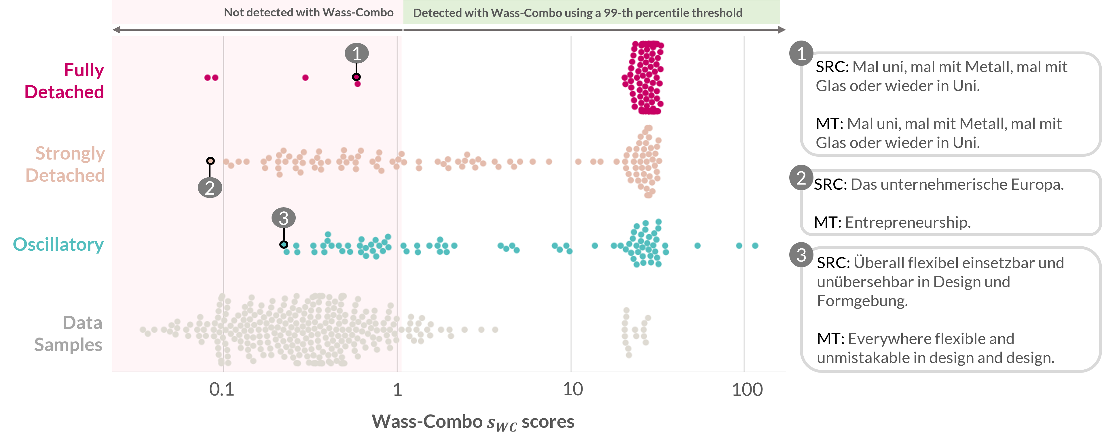
Figure 4: Distribution of Wass-Combo scores (on log-scale) for each type of hallucination and performance on a fixed-threshold scenario. We highlight three hallucinations that are not detected by Wass-Combo. These represent hallucinations in the dataset that it struggles to identify: (1) exact copies of the source sequence, (2) small level of detachment in strongly detached hallucinations, and (3) mild repetitions of 1-grams ("design").

Oscillatory Hallucinations not detected with Wass-Combo
Source	Überall flexibel einsetzbar und unübersehbar in Design und Formgebung.
Translation	Everywhere flexible and unmistakable in design and design.
Source	Um kahlen Stellen, wenn sie ohne Rüstung pg.
Translation	To dig dig digits if they have no armor pg.
Source	Damit wird, wie die Wirtschaftswissenschaftler sagen, der Nennwert vorgezogen.
Translation	This, as economists say, puts the par value before the par value.
Source	Besonders beim Reinigen des Verflüssigers kommt Ihnen dies zugute.
Translation	Especially when cleaning the liquefied liquefied liquefied.
Source	Müssen die Verkehrsmittel aus- oder abgewählt werden ?
Translation	Do you need to opt-out or opt-out of transport?
Source	Schnell drüberlesen - "Ja" auswählen und weiter gehts.
Translation	Simply press the "Yes" button and press the "Yes."
Source	Auf den jeweiligen Dorfplätzen finden sich Alt und Jung zum Schwätzchen und zum Feiern zusammen.
Translation	Old and young people will find themselves together in the village’s respective squares for fun and fun.
Source	Zur Absicherung der E-Mail-Kommunikation auf Basis von PGP- als auch X.509-Schlüsseln hat die Schaeffler Gruppe eine Zertifizierungsinfrastruktur (Public Key Infrastructure PKI) aufgebaut.
Translation	The Schaeffler Group has set up a Public Key Infrastructure PKI (Public Key Infrastructure PKI) to secure e-mail communication based on PGP and X.509 keys.

Table 13: Examples of oscillatory hallucinations randomly sampled from the set of oscillatory hallucinations not detected with Wass-Combo. Most hallucinations come in the form of mild repetitions of 1-grams or 2-grams.

Appendix H Analysis against ALTI+

Concurrently to our work, Dale et al. (2022) leveraged ALTI+ (Ferrando et al., 2022), a method that evaluates the global relative contributions of both source and target prefixes to model predictions, for detection of hallucinations. As hallucinations are translations detached from the source sequence, ALTI+ is able to detect them by identifying sentences with minimal source contribution. In Table G, we show that ALTI+ slightly outperforms Wass-Combo for fully detached hallucinations, but lags considerably behind on what comes to detecting strongly detached and oscillatory hallucinations.

Appendix I Error Analysis of Wass-Combo

We show a qualitative analysis on the same fixed-threshold scenario described in Section 6.2 in Figure 4. Differently to Figure 3, we provide examples of translations that have not been detected by Wass-Combo for the chosen threshold.

Our detector is not able to detect fully detached hallucinations that come in the form of exact copies of the source sentence. For these pathological translations, the attention map is mostly diagonal and is thus not anomalous. Although these are severe errors, we argue that, in a real-world application, such translations can be easily detected with string matching heuristics.

We also find that our detector Wass-Combo struggles with oscillatory hallucinations that come in the form of mild repetitions of 1-grams or 2-grams (see example in Figure 4). To test this hypothesis, we implemented the binary heuristic top n-gram count (Raunak et al., 2021; Guerreiro et al., 2022) to verify whether a translation is a severe oscillation: given the entire $\mathcal{D}_{\text{held}}$, a translation is flagged as an oscillatory hallucination if (i) it is in the set of 1% lowest-quality translations according to CometKiwi and (ii) the count of the top repeated 4-gram in the translation is greater than the count of the top repeated source 4-gram by at least 2. Indeed, more than $90\%$ of the oscillatory hallucinations not detected by Wass-Combo in Figure 4 were not flagged by this heuristic. We provide 8 examples randomly sampled from the set of oscillatory hallucinations not detected with Wass-Combo in Table 13. Close manual evaluation of these hallucinations further backs the hypothesis above.

Detector	ro-en			ne-en
	AUROC $\uparrow$	FPR@90TPR $\downarrow$		AUROC $\uparrow$	FPR@90TPR $\downarrow$
External Detectors
CometKiwi †	99.62	0.49		97.64	4.03
LaBSE	99.72	0.49		92.34	20.03
1-6[.4pt/2pt]      Model-based Detectors
Attn-ign-SRC	99.16	0.93		28.66	100.0
Seq-Logprob	91.97	16.42		26.38	99.94
Ours
Wass-to-Unif	99.30	0.46		81.49	64.23
Wass-to-Data	96.54 0.07	10.36 0.30		90.18 0.13	48.52 2.64
Wass-Combo	98.75 0.06	0.46 0.00		90.16 0.13	48.52 2.64

Table 14: Performance of all hallucination detectors. For Wass-to-Data and Wass-Combo We present the mean and standard deviation (in subscript) scores across five random seeds. ^†CometKiwi has been trained on these MLQE-PE data samples.

Appendix J Experiments on the MLQE-PE dataset

In order to establish the broader validity of our model-based detectors, we present an analysis on their performance for other NMT models and on mid and low-resource language pairs. Overall, the detectors exhibit similar trends to those discussed in the main text (Section 6).

J.1 Model and Data

The dataset from Guerreiro et al. (2022) analysed in the main text is the only available dataset that contains human annotations of hallucinated translations. Thus, in this analysis we will have to make use of other human annotations to infer annotations for hallucinations. For that end, we follow a similar setup to that of Tang et al. (2022) and use the MLQE-PE dataset (Fomicheva et al., 2022)— that has been reported to contain low-quality translations and hallucinations for ne-en and ro-en (Specia et al., 2021)— to test the performance of our detectors on these language pairs.

The ne-en and ro-en MLQE-PE datasets contain 7000 translations and their respective human quality assessments (from 1 to 100). Each translation is scored by three different annotators. As hallucinations lie at the extreme end of NMT pathologies (Raunak et al., 2021), we consider a translation to be a hallucination if at least two annotators (majority) gave it a quality score of 1. This process leads to 30 hallucinations for ne-en and 237 hallucinations for ro-en. Although the number of hallucinations for ne-en is relatively small, we decide to also report experiments on this language pair because the type of hallucinations found for ne-en is very different to those found for ro-en: almost all ne-en hallucinations are oscillatory, whereas almost all ro-en are fully detached.

To obtain all model-based information required to build the detectors, we use the same Transformer models that generated the translations in the datasets in consideration. All details can be found in Fomicheva et al. (2022) and the official project repository. Moreover, to build our held-out databases of source mass distributions, we used readily available Europarl data (Koehn, 2005) for ro-en ($\sim$100k samples), and filtered Nepali Wikipedia monolingual data used in (Koehn et al., 2019) for ne-en ($\sim$80k samples).

J.2 Results

The trends in Section 6.1 hold for other language pairs.

The results in Table I establish the broader validity of our detectors for other NMT models and, importantly, for mid and low-resource language pairs. Similarly to the analysis in 6.1, we find that our detectors (i) exhibit better performance than other model-based detectors with significant gains on the low-resource ne-en language pair; and (ii) can be competitive with external detectors that leverage large models.

The trends in Section 6.2 hold for other language pairs.

In Section A, we remark that almost all ne-en hallucinations are oscillatory, whereas almost all ro-en hallucinations are fully detached. With that in mind, the results in Table I establish the validity of the claims in the main-text (Section 6.2) on these language pairs: (i) detecting fully detached hallucinations is remarkably easy for most detectors, and Wass-to-Unif outperforms Wass-to-Data on this type of hallucinations (see results for ro-en); and (ii) our detectors significantly outperform all previous model-based detectors on detecting oscillatory hallucinations (see results for ne-en), which further confirms the notion that some detectors specialize on different types of hallucinations (e.g Attn-ign-SRC is particularly fit for detecting fully detached hallucinations, but it does not work for oscillatory hallucinations).

References

- Bahdanau et al. (2014) Dzmitry Bahdanau, Kyunghyun Cho, and Yoshua Bengio. 2014. Neural machine translation by jointly learning to align and translate. CoRR, abs/1409.0473.
- Berard et al. (2019) Alexandre Berard, Ioan Calapodescu, and Claude Roux. 2019. Naver labs Europe’s systems for the WMT19 machine translation robustness task. In Proceedings of the Fourth Conference on Machine Translation (Volume 2: Shared Task Papers, Day 1), pages 526–532, Florence, Italy. Association for Computational Linguistics.
- Bojar et al. (2018) Ondřej Bojar, Christian Federmann, Mark Fishel, Yvette Graham, Barry Haddow, Philipp Koehn, and Christof Monz. 2018. Findings of the 2018 conference on machine translation (WMT18). In Proceedings of the Third Conference on Machine Translation: Shared Task Papers, pages 272–303, Belgium, Brussels. Association for Computational Linguistics.
- Cheng et al. (2022) Xiaoyu Cheng, Maoxing Wen, Cong Gao, and Yueming Wang. 2022. Hyperspectral anomaly detection based on wasserstein distance and spatial filtering. Remote Sensing, 14(12):2730.
- Dale et al. (2022) David Dale, Elena Voita, Loïc Barrault, and Marta R. Costa-jussà. 2022. Detecting and mitigating hallucinations in machine translation: Model internal workings alone do well, sentence similarity even better.
- Devlin et al. (2019) Jacob Devlin, Ming-Wei Chang, Kenton Lee, and Kristina Toutanova. 2019. BERT: Pre-training of deep bidirectional transformers for language understanding. In Proceedings of the 2019 Conference of the North American Chapter of the Association for Computational Linguistics: Human Language Technologies, Volume 1 (Long and Short Papers), pages 4171–4186, Minneapolis, Minnesota. Association for Computational Linguistics.
- Feng et al. (2020) Fangxiaoyu Feng, Yinfei Yang, Daniel Cer, Naveen Arivazhagan, and Wei Wang. 2020. Language-agnostic bert sentence embedding.
- Ferrando and Costa-jussà (2021) Javier Ferrando and Marta R. Costa-jussà. 2021. Attention weights in transformer NMT fail aligning words between sequences but largely explain model predictions. In Findings of the Association for Computational Linguistics: EMNLP 2021, pages 434–443, Punta Cana, Dominican Republic. Association for Computational Linguistics.
- Ferrando et al. (2022) Javier Ferrando, Gerard I. Gállego, Belen Alastruey, Carlos Escolano, and Marta R. Costa-jussà. 2022. Towards opening the black box of neural machine translation: Source and target interpretations of the transformer.
- Fomicheva et al. (2022) Marina Fomicheva, Shuo Sun, Erick Fonseca, Chrysoula Zerva, Frédéric Blain, Vishrav Chaudhary, Francisco Guzmán, Nina Lopatina, Lucia Specia, and André F. T. Martins. 2022. MLQE-PE: A multilingual quality estimation and post-editing dataset. In Proceedings of the Thirteenth Language Resources and Evaluation Conference, pages 4963–4974, Marseille, France. European Language Resources Association.
- Guerreiro et al. (2023) Nuno M. Guerreiro, Elena Voita, and André Martins. 2023. Looking for a needle in a haystack: A comprehensive study of hallucinations in neural machine translation. In Proceedings of the 17th Conference of the European Chapter of the Association for Computational Linguistics, pages 1059–1075, Dubrovnik, Croatia. Association for Computational Linguistics.
- Guerreiro et al. (2022) Nuno M. Guerreiro, Elena Voita, and André F. T. Martins. 2022. Looking for a needle in a haystack: A comprehensive study of hallucinations in neural machine translation.
- Kantorovich (2006) Leonid V Kantorovich. 2006. On the translocation of masses. Journal of mathematical sciences, 133(4):1381–1382.
- Kobayashi et al. (2020) Goro Kobayashi, Tatsuki Kuribayashi, Sho Yokoi, and Kentaro Inui. 2020. Attention is not only a weight: Analyzing transformers with vector norms. In Proceedings of the 2020 Conference on Empirical Methods in Natural Language Processing (EMNLP), pages 7057–7075, Online. Association for Computational Linguistics.
- Kocmi et al. (2022) Tom Kocmi, Rachel Bawden, OndÅ™ej Bojar, Anton Dvorkovich, Christian Federmann, Mark Fishel, Thamme Gowda, Yvette Graham, Roman Grundkiewicz, Barry Haddow, Rebecca Knowles, Philipp Koehn, Christof Monz, Makoto Morishita, Masaaki Nagata, Toshiaki Nakazawa, Michal Novák, Martin Popel, Maja Popović, and Mariya Shmatova. 2022. Findings of the 2022 conference on machine translation (wmt22). In Proceedings of the Seventh Conference on Machine Translation, pages 1–45, Abu Dhabi. Association for Computational Linguistics.
- Koehn (2005) Philipp Koehn. 2005. Europarl: A parallel corpus for statistical machine translation. In Proceedings of Machine Translation Summit X: Papers, pages 79–86, Phuket, Thailand.
- Koehn et al. (2019) Philipp Koehn, Francisco Guzmán, Vishrav Chaudhary, and Juan Pino. 2019. Findings of the WMT 2019 shared task on parallel corpus filtering for low-resource conditions. In Proceedings of the Fourth Conference on Machine Translation (Volume 3: Shared Task Papers, Day 2), pages 54–72, Florence, Italy. Association for Computational Linguistics.
- Lee et al. (2018) Katherine Lee, Orhan Firat, Ashish Agarwal, Clara Fannjiang, and David Sussillo. 2018. Hallucinations in neural machine translation.
- Müller et al. (2020) Mathias Müller, Annette Rios, and Rico Sennrich. 2020. Domain robustness in neural machine translation. In Proceedings of the 14th Conference of the Association for Machine Translation in the Americas (Volume 1: Research Track), pages 151–164, Virtual. Association for Machine Translation in the Americas.
- Müller and Sennrich (2021) Mathias Müller and Rico Sennrich. 2021. Understanding the properties of minimum Bayes risk decoding in neural machine translation. In Proceedings of the 59th Annual Meeting of the Association for Computational Linguistics and the 11th International Joint Conference on Natural Language Processing (Volume 1: Long Papers), pages 259–272, Online. Association for Computational Linguistics.
- Ott et al. (2019) Myle Ott, Sergey Edunov, Alexei Baevski, Angela Fan, Sam Gross, Nathan Ng, David Grangier, and Michael Auli. 2019. fairseq: A fast, extensible toolkit for sequence modeling. In Proceedings of the 2019 Conference of the North American Chapter of the Association for Computational Linguistics (Demonstrations), pages 48–53, Minneapolis, Minnesota. Association for Computational Linguistics.
- Paty and Cuturi (2019) François-Pierre Paty and Marco Cuturi. 2019. Subspace robust wasserstein distances. In International conference on machine learning, pages 5072–5081. PMLR.
- Pedregosa et al. (2011) F. Pedregosa, G. Varoquaux, A. Gramfort, V. Michel, B. Thirion, O. Grisel, M. Blondel, P. Prettenhofer, R. Weiss, V. Dubourg, J. Vanderplas, A. Passos, D. Cournapeau, M. Brucher, M. Perrot, and E. Duchesnay. 2011. Scikit-learn: Machine learning in Python. Journal of Machine Learning Research, 12:2825–2830.
- Perez et al. (2022) Ethan Perez, Saffron Huang, Francis Song, Trevor Cai, Roman Ring, John Aslanides, Amelia Glaese, Nat McAleese, and Geoffrey Irving. 2022. Red teaming language models with language models. arXiv preprint arXiv:2202.03286.
- Peyré et al. (2019) Gabriel Peyré, Marco Cuturi, et al. 2019. Computational optimal transport: With applications to data science. Foundations and Trends® in Machine Learning, 11(5-6):355–607.
- Peyré and Cuturi (2018) Gabriel Peyré and Marco Cuturi. 2018. Computational optimal transport.
- Popović (2016) Maja Popović. 2016. chrF deconstructed: beta parameters and n-gram weights. In Proceedings of the First Conference on Machine Translation: Volume 2, Shared Task Papers, pages 499–504, Berlin, Germany. Association for Computational Linguistics.
- Raganato and Tiedemann (2018) Alessandro Raganato and Jörg Tiedemann. 2018. An analysis of encoder representations in transformer-based machine translation. In Proceedings of the 2018 EMNLP Workshop BlackboxNLP: Analyzing and Interpreting Neural Networks for NLP, pages 287–297, Brussels, Belgium. Association for Computational Linguistics.
- Raunak et al. (2021) Vikas Raunak, Arul Menezes, and Marcin Junczys-Dowmunt. 2021. The curious case of hallucinations in neural machine translation. In Proceedings of the 2021 Conference of the North American Chapter of the Association for Computational Linguistics: Human Language Technologies, pages 1172–1183, Online. Association for Computational Linguistics.
- Raunak et al. (2022) Vikas Raunak, Matt Post, and Arul Menezes. 2022. Salted: A framework for salient long-tail translation error detection.
- Rei et al. (2020) Ricardo Rei, Craig Stewart, Ana C Farinha, and Alon Lavie. 2020. COMET: A neural framework for MT evaluation. In Proceedings of the 2020 Conference on Empirical Methods in Natural Language Processing (EMNLP), pages 2685–2702, Online. Association for Computational Linguistics.
- Rei et al. (2022) Ricardo Rei, Marcos Treviso, Nuno M. Guerreiro, Chrysoula Zerva, Ana C. Farinha, Christine Maroti, José G. C. de Souza, Taisiya Glushkova, Duarte M. Alves, Alon Lavie, Luisa Coheur, and André F. T. Martins. 2022. Cometkiwi: Ist-unbabel 2022 submission for the quality estimation shared task.
- Reimers and Gurevych (2019) Nils Reimers and Iryna Gurevych. 2019. Sentence-bert: Sentence embeddings using siamese bert-networks. In Proceedings of the 2019 Conference on Empirical Methods in Natural Language Processing. Association for Computational Linguistics.
- Specia et al. (2021) Lucia Specia, Frédéric Blain, Marina Fomicheva, Chrysoula Zerva, Zhenhao Li, Vishrav Chaudhary, and André F. T. Martins. 2021. Findings of the WMT 2021 shared task on quality estimation. In Proceedings of the Sixth Conference on Machine Translation, pages 684–725, Online. Association for Computational Linguistics.
- Staerman et al. (2021) Guillaume Staerman, Pierre Laforgue, Pavlo Mozharovskyi, and Florence d’Alché Buc. 2021. When ot meets mom: Robust estimation of wasserstein distance. In International Conference on Artificial Intelligence and Statistics, pages 136–144. PMLR.
- Tang et al. (2022) Joël Tang, Marina Fomicheva, and Lucia Specia. 2022. Reducing hallucinations in neural machine translation with feature attribution.
- Vaswani et al. (2017) Ashish Vaswani, Noam Shazeer, Niki Parmar, Jakob Uszkoreit, Llion Jones, Aidan N Gomez, Ł ukasz Kaiser, and Illia Polosukhin. 2017. Attention is all you need. In Advances in Neural Information Processing Systems, volume 30. Curran Associates, Inc.
- Villani (2009) Cédric Villani. 2009. Optimal transport: old and new, volume 338. Springer.
- Voita et al. (2021) Elena Voita, Rico Sennrich, and Ivan Titov. 2021. Analyzing the source and target contributions to predictions in neural machine translation. In Proceedings of the 59th Annual Meeting of the Association for Computational Linguistics and the 11th International Joint Conference on Natural Language Processing (Volume 1: Long Papers), pages 1126–1140, Online. Association for Computational Linguistics.
- Wang and Sennrich (2020) Chaojun Wang and Rico Sennrich. 2020. On exposure bias, hallucination and domain shift in neural machine translation. In Proceedings of the 58th Annual Meeting of the Association for Computational Linguistics, pages 3544–3552, Online. Association for Computational Linguistics.
- Wang et al. (2021) Yinan Wang, Wenbo Sun, Jionghua Jin, Zhenyu Kong, Xiaowei Yue, et al. 2021. Wood: Wasserstein-based out-of-distribution detection. arXiv preprint arXiv:2112.06384.
- Yan et al. (2021) Yongzhe Yan, Stefan Duffner, Priyanka Phutane, Anthony Berthelier, Christophe Blanc, Christophe Garcia, and Thierry Chateau. 2021. 2d wasserstein loss for robust facial landmark detection. Pattern Recognition, 116:107945.
- Zerva et al. (2022) Chrysoula Zerva, Frédéric Blain, Ricardo Rei, Piyawat Lertvittayakumjorn, José G. C. de Souza, Steffen Eger, Diptesh Kanojia, Duarte Alves, Constantin Orǎsan, Marina Fomicheva, André F. T. Martins, and Lucia Specia. 2022. Findings of the WMT 2022 shared task on quality estimation. In Proceedings of the Seventh Conference on Machine Translation, pages 69–99, Abu Dhabi. Association for Computational Linguistics.
- Zhou et al. (2021) Chunting Zhou, Graham Neubig, Jiatao Gu, Mona Diab, Francisco Guzmán, Luke Zettlemoyer, and Marjan Ghazvininejad. 2021. Detecting hallucinated content in conditional neural sequence generation. In Findings of the Association for Computational Linguistics: ACL-IJCNLP 2021, pages 1393–1404, Online. Association for Computational Linguistics.