Taming Lagrangian Chaos with Multi-Objective Reinforcement Learning

Abstract

We consider the problem of two active particles in 2D complex flows with the multi-objective goals of minimizing both the dispersion rate and the energy consumption of the pair. We approach the problem by means of Multi Objective Reinforcement Learning (MORL), combining scalarization techniques together with a Q-learning algorithm, for Lagrangian drifters that have variable swimming velocity. We show that MORL is able to find a set of trade-off solutions forming an optimal Pareto frontier. As a benchmark, we show that a set of heuristic strategies are dominated by the MORL solutions. We consider the situation in which the agents cannot update their control variables continuously, but only after a discrete (decision) time, $\tau$. We show that there is a range of decision times, in between the Lyapunov time and the continuous updating limit, where Reinforcement Learning finds strategies that significantly improve over heuristics. In particular, we discuss how large decision times require enhanced knowledge of the flow, whereas for smaller $\tau$ all a priori heuristic strategies become Pareto optimal.

1 Introduction

In many engineering and geophysical applications robotic instruments are often used for multi-agent sensing e.g. where a fleet of instrumented drifters is used to collect information in the ocean, multi-robots are used for searching sources leaking hazardous substances, or to probe complex environments Lermusiaux_JMR ; ELOR201276 ; WuWencen ; Schmickl ; Bechinger_2016 . A typical application is how to keep the fleet under control, e.g., for patrolling the same region, keeping a given geometric formation and/or following a predetermined point-to-point path. In typical flows, the relative distance between two passive drifters would always grow, either exponentially, due to Lagrangian chaos when they are close, or in a diffusive way at large scales, when non-linear effects become dominant crisanti1991lagrangian ; cencini2010chaos . Animal behaviour is often an inspiration and a leading direction of research trying to develop bio-mimetic strategies ginelli2016physics ; Marchetti ; Ballerini_birdflocks . However, it is unclear whether using heuristic hard-wired rules would be enough to control the swarm in the presence of a strongly mixing flow khurana2013stability . Moreover, in many realistic applications, agents need to take into account of strong engineering or biological limitations, needing to actively learn how to take advantage of the flow to accomplish the goal. As a result, we search to develop active complex policies to control complex environments. In chaotic or turbulent flows, the problem is given by the strong sensitivity of the system to any perturbation, making the very meaning of optimal control a fragile notion. In this direction, a few attempts to control single Lagrangian instrumented particles via Reinforcement Learning (RL) algorithms have been proposed to solve the Zermelo’s optimal navigation problem of reaching a fixed target Biferale_2019 ; Buzzicotti_Zermelo2020 ; bec2020 . Moreover, RL has been successfully employed to optimize the soaring of a glider in thermal currents Reddy_PNAS ; reddy_nature and to harness wind for airborne energy celani-airborne . Recently, adversarial games between two competing agents have also been proposed to study chase-and-escape fish strategies at low Reynolds number Borra_2022 .

In this paper, we consider two agents (a particle pair) transported by a flow and having some limited knowledge on the underlying flow, which should act collectively so as to contrast the growth of their separation and, at the same time, to minimize as much as possible the cost for control. We assumed to solve the problem when the two particles stay at distances where the flow is differentiable so that, without control, their separation would grow exponentially due to Lagrangian chaos. To improve realism, we model the problem imposing limitations in detection (partial observability) and in the possible actions to undertake (partial maneuverability). Namely, we allow each agent to sample only few local properties of the underlying flow and to receive information about the other one only at given decision times, spaced by an interval $\tau$, in order to update their actions. For what concerns the actions, following bec2020 we suppose that the two objects can swim either along the direction of their separation or in the perpendicular one, with a variable speed. Finally, to be able to fulfill the objective to minimize the energy cost, we also include the action of no-swimming to allow the couple of particles to learn when to be passively transported by the current, if useful Buzzicotti_Zermelo2020 . As a result, we have a multi-agent (2 Lagrangian pair) and a multi-task (minimize both chaotic dispersion and energy consumption) problem Coello_1 . We approach this typical long-term optimization problem with conflicting objectives by using Multi-Objective Reinforcement Learning (MORL) algorithms Coello_2 ; MORL_overview ; Vamplew_MORL . Indeed, in the classical single-task RL the reward is a scalar, whereas in MORL the reward is a vector, with an element for each objective. We approach MORL via scalarization, i.e. by defining a new scalar total reward by a weighted sum along all the element of the original reward vector Natarajan_scalarization ; Castelletti_scalarization . For this reason, there exists a set of trade-off solutions forming the so called Pareto frontier Vamplew_Pareto ; Zitzler_Pareto , where each solution on the frontier is Pareto Efficient, i.e. no single objective can be made better off without making at least another one worse off.

Using this approach, we show how to find a set of Pareto optimal policies to efficiently minimize both chaotic dispersion and swimming cost. To benchmark these strategies we will compare them to a set of heuristic baselines. In particular, we show how the learned strategies are able to exploit nontrivial information of the underlying flow.

The paper is organized as follows. In Sec.2, we describe the general setup of the problem: the model of the Lagrangian pair, how they can act and sense the environment, and the details of the underlying fluid flow. In Sec.3 we introduce the concepts of MORL giving details on our choice for the reward function and the learning protocol. Furthermore, we present the concepts of Pareto dominance and Pareto frontier. In Sec.4, we discuss the main results including a heuristic analysis focused on explaining the role of the decision time. Finally, we give our conclusion in Sec.5.

2 The model

2.1 Active control of Lagrangian pairs in a flow

In typical flows, Lagrangian chaos crisanti1991lagrangian ; cencini2010chaos causes an exponential growth of the separation, $\delta X(t)=\|\bm{X}_{2}(t)-\bm{X}_{1}(t)\|$, between pairs of (uncontrolled) tracer particles that are initially very close, i.e. $\langle\ln\delta X(t)\rangle\simeq\ln\delta(X(0))+\lambda t$ , ($\lambda$ being the Lagrangian Lyapunov exponent). Our goal here is to develop strategies for instrumented particles to control and, possibly, minimize such chaotic dispersion and at the same time to save energy. In particular, we consider particles in the one-way coupling approximation and an autonomous propelling mechanism with a speed $V(t)$ in the direction $\hat{\bm{p}}(t)$ superimposed to the transport by the flow. Thus we assume the particles to obey the following equations of motion:

$$\begin{cases}\dot{\bm{X}_{\alpha}}=\bm{u}(\bm{X}_{\alpha}(t),t)+\bm{U}_{\alpha}^{ctrl}(t)\,,\\ \bm{U}_{\alpha}^{ctrl}(t)=V_{\alpha}(t)\bm{\hat{p}}_{\alpha}(t),\end{cases}\,$$ (1)

where $\alpha=1,2$ is the agent’s index, $\bm{u}(\bm{X}_{\alpha}(t),t)$ is the velocity of the underlying 2D advecting flow and $\bm{U}_{\alpha}^{ctrl}(t)$ is the control contribution to the particle velocity.

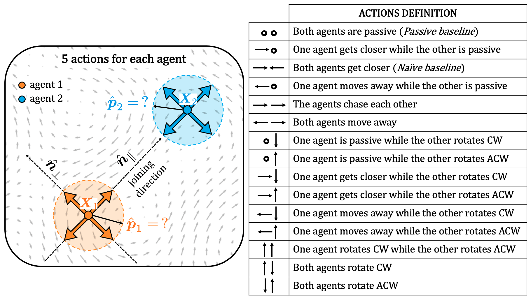
Figure 1: (Left) The $5$ possible actions available to each agent, namely: remain passive or swim in the longitudinal direction $\pm\bm{\hat{n}}_{\parallel}$ or in the transversal one $\pm\bm{\hat{n}}_{\perp}$. (Right) Scheme of the set of $15$ actions for the couple of agents, obtained after removing symmetrical action pairs. Besides the longitudinal actions, choosing the transversal directions allows the agents to rotate with respect to each other clock-wise (CW) or anti-clockwise (ACW).

We assume the agents to interact with the environment and between each other only every $\tau$ time units. At each decision time the agents can measure some flow properties (a proxy for the environmental state) and sense their mutual separation. Then, on the basis of the information received, they can decide their action, i.e. choose the swimming intensity and direction. In this way, the control $\bm{U}_{\alpha}^{ctrl}(t)$ becomes a piece-wise constant in time function, i.e. $\hat{\bm{p}}_{\alpha}(t)=\hat{\bm{p}}_{\alpha}(t_{j})$ and $V_{\alpha}(t)=V_{\alpha}(t_{j})$ for $t_{j}\leq t<t_{j}+\tau$, with $t_{j}=j\tau$ being the $j^{th}$ decision time. Clearly, an important role in achieving successfully strategies for staying close is played by the dimensionless combination of the two parameters $\tau\,\lambda$. When $\tau\lambda>1$ the control is too sporadic and the velocity field can separate considerably the agents. On the other hand, for $\tau\lambda\to 0$,the control problem becomes easier.

Concerning the swimming directions, $\hat{\bm{p}}_{\alpha}(t)$, we assume that the agents have a limited set of choices. Namely, similarly to bec2020 , the agents can either swim along their longitudinal (joining) direction ($\hat{\bm{n}}_{\parallel}$) or in the transversal one ($\hat{\bm{n}}_{\perp}$). Where $\hat{\bm{n}}_{\parallel}=({\bm{X}_{2}-\bm{X}_{1}})/{\delta X}$ and $\hat{\bm{n}}_{\perp}\cdot\hat{\bm{n}}_{\parallel}=0$ (see Fig. 1). We set the swimming intensity, $V_{\alpha}(t)$ to be proportional to the agent distance (measured at the decision time), i.e.

$$V_{\alpha}(t)=F_{\alpha}(t)\delta X(t)\,,$$ (2)

and we let each agent to choose either to turn on the control by actively swimming, $F_{\alpha}(t)=f>0$, or to turn it off, $F_{\alpha}(t)=0$, to save energy. With this choice, the first objective is connected to minimize the Lyapunov exponent of the controlled system. On the other hand, had we used a constant swimming speed, would have introduced a typical threshold distance above/below which the agents will always be able to control/not-control, at least, for small values of $\tau$. Furthermore, to study the problem in a more challenging way, we assume that swimming cannot completely overcome the dynamics, i.e. $2f\lesssim\lambda$ (see below).

Summarizing, at each decision time $t_{j}$, agent $\alpha$ can pick any of $5$ actions, $a\in\{F_{\alpha}(t_{j})=0;F_{\alpha}(t_{j})=f$ with $\hat{\bm{p}}_{\alpha}=\pm\hat{\bm{n}}_{\parallel},\pm\hat{\bm{n}}_{\perp}\}$ namely, the agents can choose either to be passive or to swim along their longitudinal or perpendicular directions. We will call naïve policy the strategy where the agents always choose to navigate towards each other, i.e. $\hat{\bm{p}}_{1}=\hat{\bm{n}}_{\parallel}$ and $\hat{\bm{p}}_{2}=-\hat{\bm{n}}_{\parallel}$. Likewise, we will call passive policy the strategy when $F_{1}=F_{2}=0$. In principle, a set of $5^{2}=25$ actions is available for the couple of agents. However, the space of actions can be reduced by removing symmetries (e.g. the configuration in which $\hat{\bm{p}}_{1}=\hat{\bm{n}}_{\parallel}$ and the second is passive is equivalent to the configuration in which the first agent is passive and $\hat{\bm{p}}_{2}=-\hat{\bm{n}}_{\parallel}$). In this way, the set of actions for the couple reduces to the set $\mathcal{A}$ of 15 actions shown in Fig.1.

2.2 Sensing the environment

Besides their relative position and distance, at each decision time, the agents receive some cues on the fluid environmental state. Concerning the observability of the environment, assuming that they are close enough for the field to be smooth, we imagine the two agents can have only a rough estimates of the relative longitudinal and transverse gradients, defined as

$$\sigma_{\parallel}=\frac{(\bm{u}(\bm{X}_{2},t)-\bm{u}(\bm{X}_{1},t))}{\delta X}\cdot\hat{\bm{n}}_{\parallel}\,$$ (3)

$$\sigma_{\perp}=\frac{(\bm{u}(\bm{X}_{2},t)-\bm{u}(\bm{X}_{1},t))}{\delta X}\cdot\hat{\bm{n}}_{\perp}\,,$$ (4)

which can be obtained by exchanging information about their local velocities. To further restrict the state-space, we suppose that the agents are able to measure their velocity difference and separation, as gradients approximation, with a limited sensitivity and we restrict the set of values of $\sigma_{\perp},\sigma_{\parallel}$ to 4 states for each one of them, for a total of 16 discretized states, labeling whether the underlying flow brings them closer or farther away (longitudinal gradients) and in which direction it rotates them (transverse gradients) see Fig. 2 for a summary of all states. The value of the discretization constant $c$ is chosen such as all the $16$ states are sufficiently visited ($c=2.8$ in our case).

Figure 2: Definition of the 16 states, obtained from the discretization of longitudinal (3) and transversal (4) gradients. The former informs about the local rate of expansion/contraction due to the flow, the latter tells the rate of clock-wise (CW) or anti-clockwise (ACW) rotation imposed by the flow on the joining direction. In figure is shown the states discretization, with $c$ a discretization constant.

2.3 The space of control policies

Given 15 actions and 16 states we have a possible set of $15^{16}$ deterministic policies $[\pi:s\to a]$, making the brute force optimization search impossible: one has to resort to Reinforcement Learning techniques (as discussed in Sec. 3). However, there is an intuitive way to trace back to a reduced policies space that can be analyzed systematically as a set of hardwired baseline policies. By restricting perceptions to the longitudinal components (3) we can assume that only the actions along the joining direction are important. Considering only the first three actions in the right panel in Fig.1, we get to a $3^{4}=81$ reduced set. In the following, we will consider these $81$ policies as our reference heuristics to benchmark the one found by our MORL implementation.

2.4 Model flow

As for the fluid environment, we used a 2D homogeneous, (nearly) isotropic, incompressible and time-dependent flow as in Ref. bec2005 . In particular, the velocity field is defined in terms of a stream function, $\bm{u}(\bm{x},t)=\nabla_{\perp}\psi(\bm{x},t)=(\partial_{y}\psi,-\partial_{x}\psi)\,,$ which is expressed as a superposition of few Fourier modes,

$$\psi(\bm{x},t)=\sum_{\bm{k}\in{\mathcal{K}}}{(A(\bm{k},t)e^{i\,\bm{k}\cdot\bm{x}}+cc.)\,,}$$ (5)

${\mathcal{K}}=\{(\frac{2\pi}{L},0),(\pm\,\frac{2\pi}{L},\frac{2\pi}{L}),(0,\frac{2\pi}{L})\}$, where $L$ is the scale periodicity of the flow. In (5) $A(\bm{k},t)=A_{r}(\bm{k},t)+i\,A_{i}(\bm{k},t)$ are random and time-dependent amplitudes obtained from an Ornstein-Uhlenbeck process OUprocess

$$\dot{A}_{\beta}(\bm{k},t)=-\frac{1}{\tau_{f}}A_{\beta}(\bm{k},t)+\Big{(}\frac{2\sigma^{2}(\bm{k})}{\tau_{f}}\Big{)}^{1/2}\eta_{\beta}(\bm{k},t)\,,$$ (6)

with $\beta=r,i$. Where $\tau_{f}$ sets the flow correlation time, $\eta_{\beta}(\bm{k},t)$ are zero-mean Gaussian variables with correlation $\langle\eta_{\alpha}(\bm{k},t)\eta_{\beta}(\bm{k}^{\prime},t^{\prime})\rangle=\delta_{\alpha,\beta}\delta_{\bm{k},\bm{k}^{\prime}}\delta(t-t^{\prime})$ , and $\sigma^{2}(\bm{k})=\frac{u^{2}_{rms}}{2\|\bm{k}\|^{2}}$. We fixed $\tau_{f}=1,L=1,u_{rms}=1$. With this choice the maximum Lyapunov exponent characterizing the mean exponential rate of divergence between two (uncontrolled) tracers particles is $\lambda\simeq 1.4$.

3 Reinforcement learning and multi-objective optimization

Starting from our set of states and actions, our aim is to solve an optimization problem with two objectives: minimizing both the rate of separation growth and the energy consumption. We are thus in the field of competing Multi-Objective Optimization (MOO) Coello_1 ; Coello_2 . The optimality of such solutions can be defined in terms of Pareto dominance Vamplew_MORL ; Zitzler_Pareto , namely a solution dominates another if it is superior on at least one objective and at least equal on all others. For instance, in Fig.3 a) the solutions $A$ and $B$ dominate $C$, whereas $A$ and $B$ are incomparable, because each is superior in at least one objective. All the dominating solutions form the Pareto frontier Vamplew_MORL ; Zitzler_Pareto , depicted with black circles in Fig.3 b).

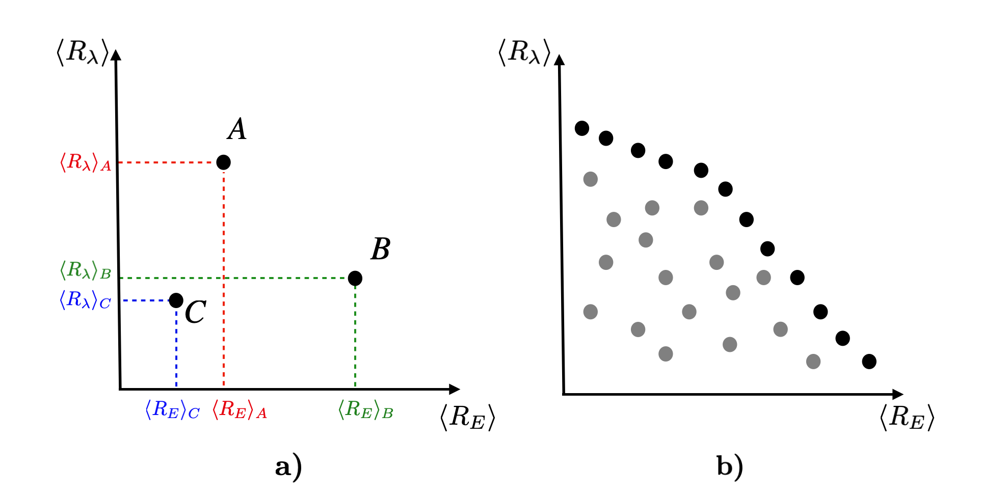
Figure 3: Concepts of Pareto dominance (a) and Pareto frontier (b). $\langle R_{\lambda}\rangle$ and $\langle R_{E}\rangle$ represent the two single objectives of minimizing particle separation and power consumption.

Reinforcement Learning (RL) algorithms sutton2018reinforcement aim at maximizing a single scalar reward usually representing a single long-term objective. MOO can also be obtained within standard RL algorithms such as, e.g., Q-learning sutton2018reinforcement by scalarization, formulating a “new” total single-objective optimization problem obtained as a weighted sum of each sub-objective functions Natarajan_scalarization ; Castelletti_scalarization . By solving the scalar optimization problem at varying the weights in the sum one can find the Pareto optimal solutions to the MOO. Following this idea, we define a different reward function for each of the two competing sub-problems.

The first allows the agents to judge their performance in controlling the separation rate:

$$r_{\lambda}(t_{j})=-\frac{1}{T_{max}}\ln\Big{(}\frac{\delta X(t_{j})}{\delta X(t_{j}-\tau)}\Big{)}\,,$$ (7)

which penalizes actions that, between two consecutive decisions, cause an increase of the distance, and where $T_{max}$ is a fixed time horizon that we considered as terminal state for the learning episodes and chosen such that the relative distance between the two particles is always in the linear regime ($T_{max}=5.5$ in our case). Notice that summing the reward (7) over a whole episode

$$R_{\lambda}=\sum_{j=1}^{T_{max}/\tau}{r_{\lambda}(t_{j})}$$ (8)

when averaging over may episodes we have

$$\langle R_{\lambda}\rangle=-\frac{1}{T_{max}}\Big{\langle}\frac{\delta X(T_{max})}{\delta X(0)}\Big{\rangle}\simeq-\lambda_{c}\,.$$ (9)

Thus, the optimization problem restricted to this reward would be solved by the policy which minimizes the Lyapunov exponent of the controlled system, $\lambda_{c}$.

The second reward function informs the agent about the energy cost:

$$r_{E}(t_{j})=-\frac{1}{T_{max}}\lambda\tau N_{a}(t_{j})\,$$ (10)

where $N_{a}(t_{j})(=0,1,2)$ counts the number of agents which have selected any of the actions ‘swim’; we have introduced a normalization term $\lambda\tau$ to have two rewards of the same order of magnitude (on average we can estimate $r_{\lambda}=(\tau\lambda)/T_{max}$).

For the multi objective optimization, we need to combine (7) and (10) through a scalarization parameter, $\beta$:

$$r_{tot}(t_{j})=r_{\lambda}{(t_{j})}+\beta r_{E}(t_{j})\,$$ (11)

and consider many single-objective problems for $r_{tot}$ at varying $\beta$. Therefore, at each decision time, the Lagrangian pair receives a shared reward, $r_{tot}$. For each $\beta$ the goal is to find the policy maximizing the cumulative total reward,

$$R_{tot}=\sum_{j=1}^{T_{max}/\tau}[r_{\lambda}(t_{j})+\beta\,r_{E}(t_{j})]=R_{\lambda}+\beta R_{E}\,.$$ (12)

From the above expression there are two clear limits: $\beta\rightarrow 0$ and $\beta\rightarrow\infty$. In the former limit we minimize particle distance without caring on energy consumption, a goal that is not obvious per se and will depend on the decision time, $\tau$. The latter case is simpler, because as the cost of swimming increases the best policy is the passive one. How does the transition between these two limiting regimes take place is the question that we are going to answer in Sec.4 by studying the Pareto frontier of our multi-task problem. See Appendix A for details of the Q-learning algorithm that we have implemented.

Due to learning stochasticity and the fact that the performances of different policies can be very close, to find the best solutions we performed $100$ independent learning sections (i.e. using different initialization seeds) for each scalarization parameter $\beta$. Each learning section lasts $50000$ episodes. The 100 learned policies for each $\beta$ have been validated on 100000 different realizations of the flow. Then we assumed as best learned policies the ones that maximize the average over the validation set of (12).

4 Results

Here, we present the results. In the first section, we present a detailed analysis of the policy related to a fixed decision time value, $\tau=0.3$, which given that the uncontrolled Lyapunov exponent is $\lambda\approx 1.4$ corresponds to a case $\tau\lambda<1$ (and $\tau<\tau_{f}=1$) that allows us to control the dynamics but the interval between decision times, $\tau$, is sufficiently high to make the problem nontrivial. In the second section, we analyze specifically the role of $\tau$ presenting a heuristic analytical prediction in the $\tau\to 0$ limit and a numerical study based on the heuristic policies as a function of $\tau$. In particular, we show that the concavity of the Pareto frontier is strongly dependent on $\tau$.

To make the control non-trivial, we fix the swimming rate to $f=0.7$ so that the controlled Lyapunov exponent is never negative. We also tested smaller values obtaining qualitatively similar results.

4.1 Detailed analysis of learned policies

As discussed in Sec. 3, we approach the multi objective optimization through reinforcement learning via scalarization, that is we perform many learning processes, with the protocol described at the end of Sec. 3, by varying the scalarization parameter $\beta$ that weighs the two rewards (see (12)). In Fig. 4, we show a typical learning process for a single $\beta$ value. At the beginning of the learning phase, the Q-learning algorithm explores different random policies. After many episodes the learning parameters, $\epsilon$ and $\alpha$, decrease (see (19)-(20)) and the Q-matrix stabilizes. The inset of Fig. 4 displays the evolution of two components of the reward. As discussed, for the same $\beta$ the learning process is then repeated over $100$ trials, each learned policy is evaluated on a validation set to identify the best learned policy for that value of $\beta$.

In Fig.5, we show the mean (over the validation set) of the total cumulative reward obtained to minimize the separation, $\langle R_{\lambda}\rangle$ (9) vs the mean of the total cumulative reward obtained to save energy, $\langle R_{E}\rangle=\Big{\langle}\sum_{j=1}^{T_{max}/\tau}{r_{E}(t_{j})}\Big{\rangle}$, for different $\beta$ values. Then we can identify as optimal the solutions that dominate all the others in the sense of Pareto dominance. In particular the best learned policies for each $\beta$ are surely on the Pareto frontier (filled circles in Fig. 5). As one can see, the learned policies reach rewards that outperform the 81 heuristic policies, indicating that the RL protocol has converged to optimal solutions. The inset in Fig.5 provides a quantitative idea of the improvement with respect to the naïve and passive baseline, respectively, by showing the improvement of the best-learned policies as a function of $\beta$. One can see that the best learned policies are generically better than the baselines.

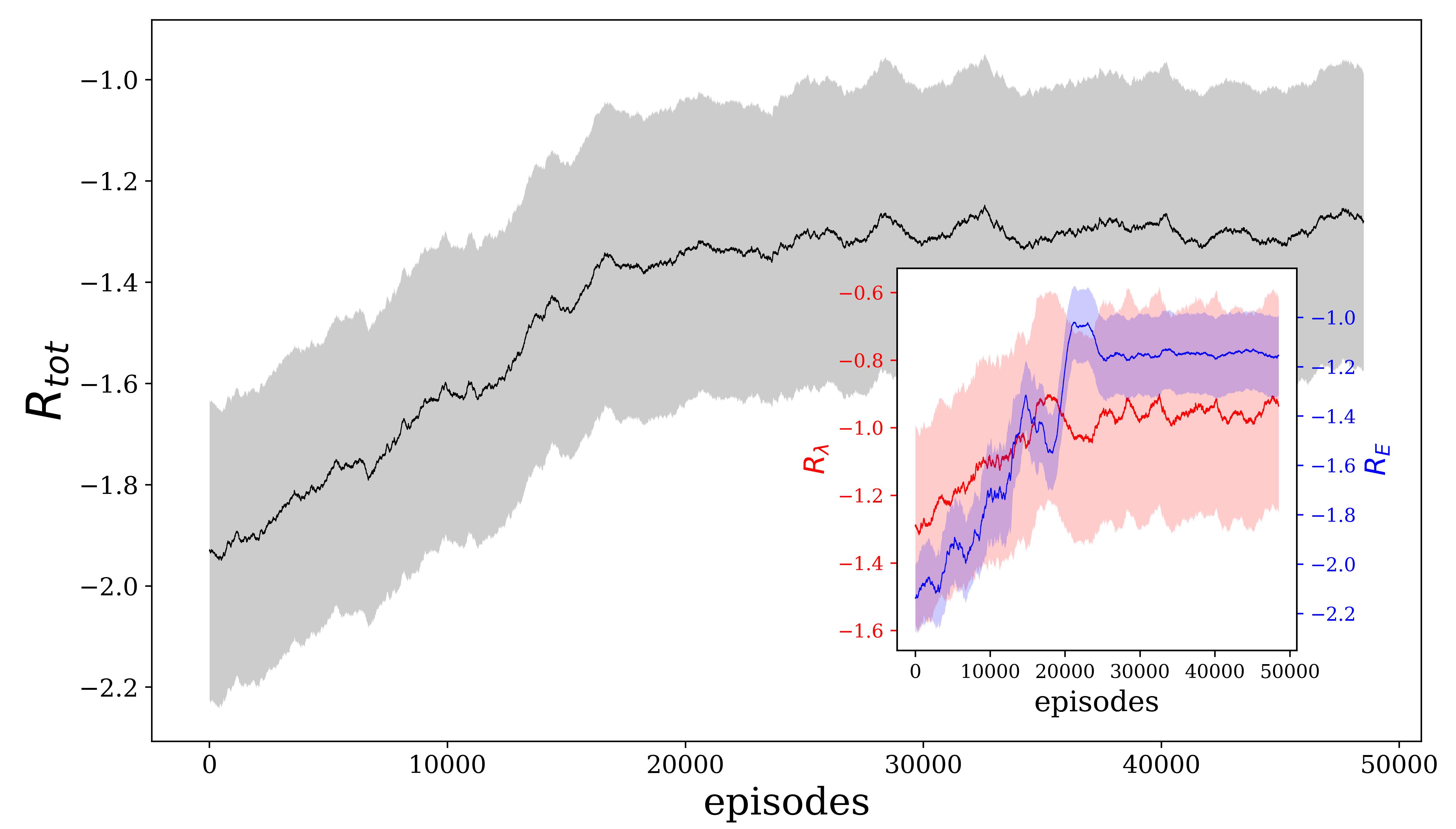
Figure 4: Example of learning process. The total reward $R_{tot}$ vs the episodes: the solid line show the running average over 1500 episodes while the gray shaded area shows the fluctuations in the individual episodes. The inset show the evolution of the two contributions to the reward $R_{\lambda}$ (red) and $R_{E}$ (blue). Data refer to one learning trial for $\beta=0.3$ and $\tau=0.3$.

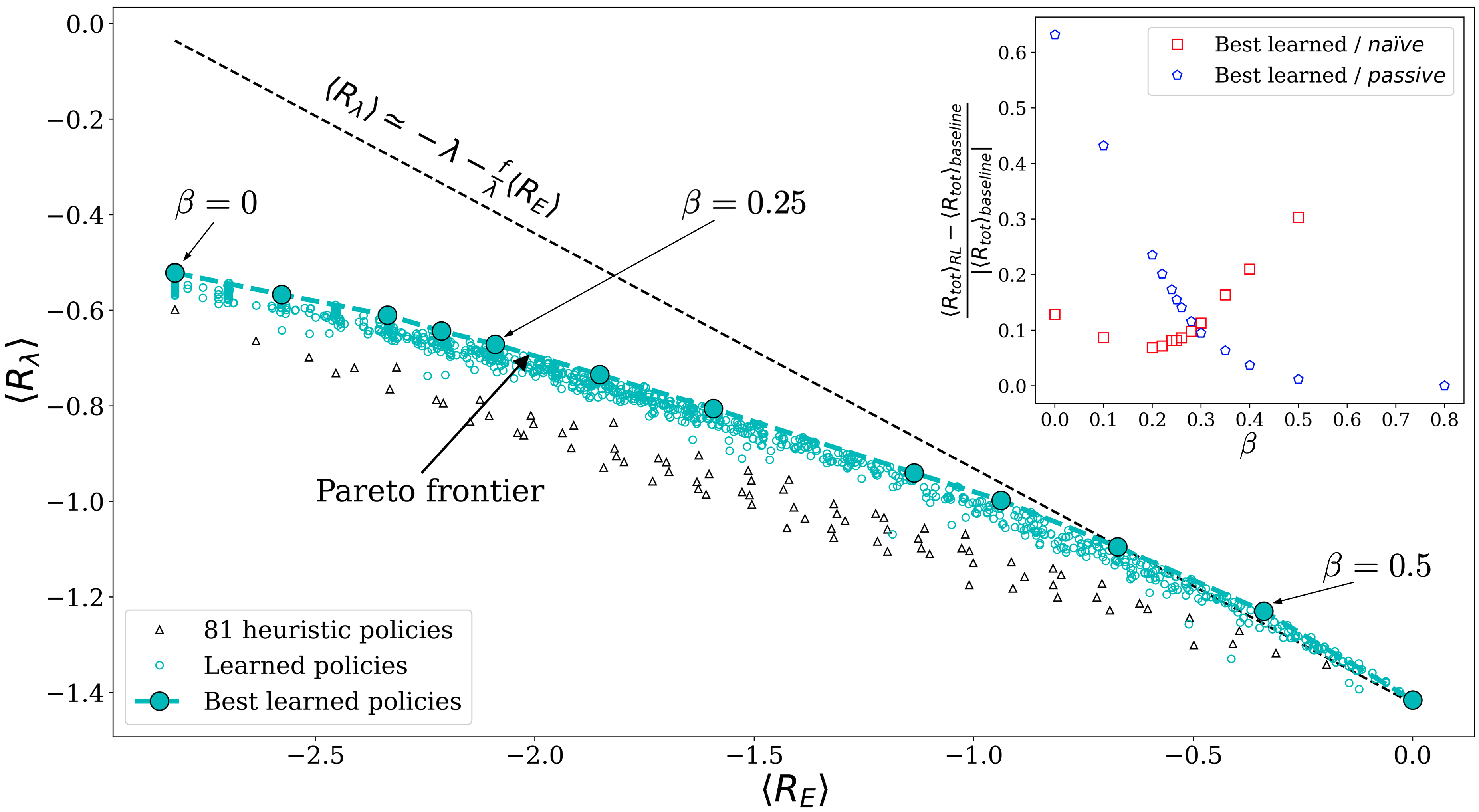
Figure 5: $\langle R_{\lambda}\rangle$ vs $\langle R_{E}\rangle$ obtained by setting the decision time $\tau=0.3$. The dashed black line indicates the highest performances that can be achieved for $\tau\rightarrow 0$ (see (15)). We show with black triangles the performances of 81 heuristic policies and with light blue circles all the policies learned from the Q-learning algorithm to solve the multi-objective problem, in particular the filled large circles show the best learned policies for each $\beta$, and the dashed blue line the Pareto frontier. One can see that learned policies dominate the heuristic ones. Inset: Relative improvement of $\langle R_{tot}\rangle$ as a function of $\beta$ of the best policies learned from RL with respect to the naïve (red squares) and passive (blue pentagon), respectively.

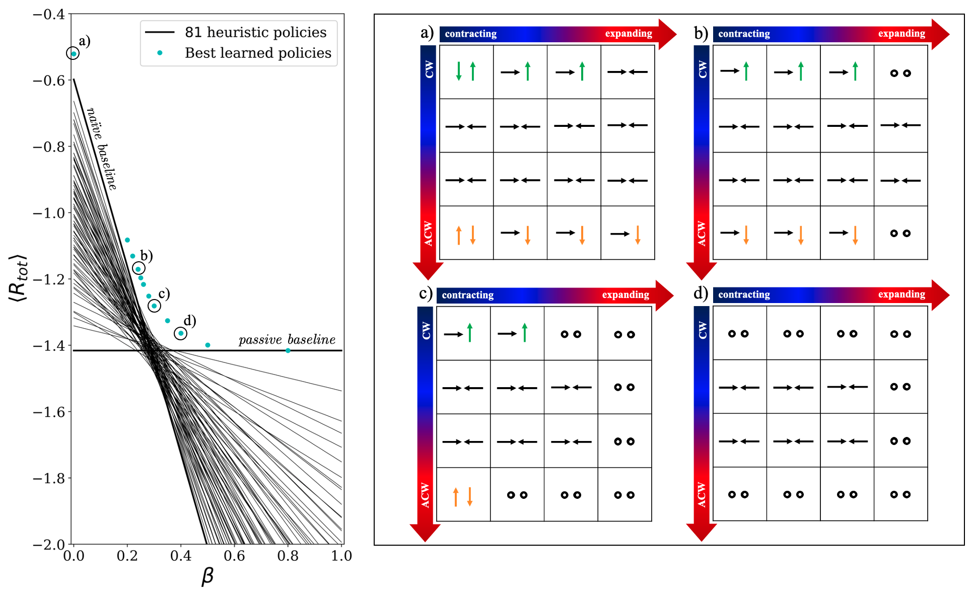
Figure 6: (Left) $\langle R_{tot}\rangle$ vs $\beta$ for different policies obtained with a decision time $\tau=0.3$. With the 81 straight lines are shown the heuristic performances, including the two extreme cases of the naïve baseline and the passive policy. It can be seen that as $\beta$ increases the naïve policy immediately get worse, while the passive policy is $\beta$-independent. In light blue are shown the best policies learned from Q-learning for each $\beta$ that improve all the heuristic performances. (Right) Pictorial representation of $4$ policies learned from RL corresponding to the circled symbols on the left. In green and orange are highlighted the ACW and CW rotation actions chosen as a counter-move with respect to the underlying flow rotation.

In particular, for $\beta=0$, since there is no cost for swimming, one might expect the naïve baseline to be a good strategy for minimizing the agents separation. Instead, we discovered that also in this limit there is a nontrivial optimal strategy for Lagrangian agents that outperform the naïve one with an improvement of $12\%$ in the maximization of the total reward. The discovered strategy is such that, when the velocity field is contracting and rotates strongly the position of one agent with respect to the other, it turns out to be more convenient to counter-rotate with respect to the rotation induced by underlying velocity field rather than to simply navigate towards each other. We can explain that as a realignment along the contracting direction. Indeed, due to the finite decision time, it is less effective to swim towards each other in the direction identified at the decision time, which is quickly changed by the flow. On the other hand, for high values of $\beta$, when swimming has a high cost, RL easily learns that the best policy is the passive one, where the two agents always switch off the engine. Other $\beta$ values lead to the transition region between these two extreme cases, where new navigation strategies are learned. In particular, as seen from the inset of Fig. 5, the region around $\beta=0.3$ seems to be the more interesting, it is thus worth analyzing the learned policies in this region.

In Fig.6(Left) we show the performance of the best learned policies for each $\beta$ in comparison with the 81 heuristic ones. Notice that for the latter it is enough to measure $\langle R_{\lambda}\rangle$ and $\langle R_{E}\rangle$ to know the value of $\langle R_{tot}\rangle$ as a function of $\beta$, obtaining 81 benchmark straight lines, as shown in Fig.6(Left). It can be seen that RL always improve the maximization of the total cumulative reward, $\langle R_{tot}\rangle$. In Fig.6(Right)a-d we show a tabular representation of some policies learned as optimal, i.e. that lie on the Pareto frontier and appertain to the region around $\beta=0.3$ (see circled dots in Fig.6(Left)). It emerges that counter-rotating with respect to the underlying flow rotation is important and that, as $\beta$ increases, is more convenient navigate when the flow is contracting rather than when it is expanding the agents’ separation; e.g. the policy in Fig.6c) shows that the Lagrangian pair choose to be passive along all the expanding states.

We end this section commenting on possible symmetries of swimming strategies. In fact, the counter-rotating action with respect to the underlying flow rotation that emerges to be important can occur both when the counter-rotation is clockwise and when it is anti-clockwise. This could lead to some ambiguity in the choice of swimming strategies or, more precisely, it could happen that equivalent strategies exist simultaneously. However, this does not seem to cause convergence issues, and RL is still able to identify optimal solutions.

4.2 Heuristic analysis

We now discuss the role of the interval between decision times, $\tau$, by relying on the set of 81 heuristic (hard-wired) strategies obtained as a reduced policies space from the 4 longitudinal states and the first 3 actions in Fig.1. Indeed, their analysis is enough to understand the qualitative effect of changing the decision time with no needed to perform any learning.

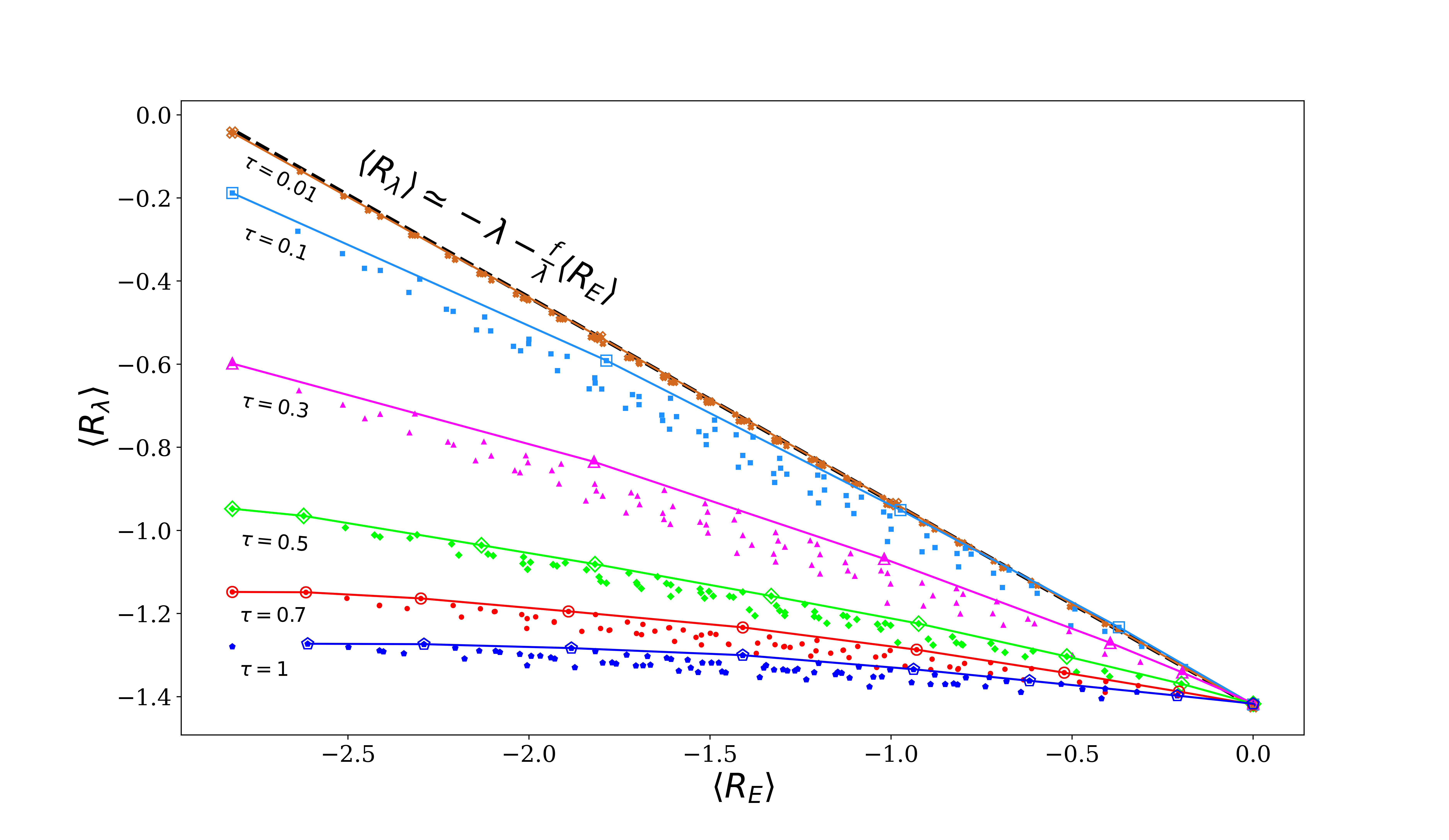
Figure 7: Pareto frontier for a reduced policies-space, which is a lower bound to the true Pareto frontier: $\langle R_{\lambda}\rangle$ vs $\langle R_{E}\rangle$ obtained varying the decision time, $\tau$ for the 81 heuristic policies. The dashed black line indicates a linear dependence between $\langle R_{\lambda}\rangle$ and $\langle R_{E}\rangle$ reached for small $\tau$. We show with empty symbols the Pareto frontier that would result for each decision time by restricting the problem to study only the $81$ heuristic policies. It can be seen that as $\tau$ increases, the frontier becomes concave.

In Fig.7 we show the same plot of Fig.5 for different values of $\tau$ and only considering the heuristic policies, taking the Pareto dominating strategies in this reduced policy space we obtain a lower bound to the true Pareto frontier, which is enough for the following analysis. Small decision values of $\tau$ correspond to frequent measurements of the system and thus, as intuition would suggest, to major adjustments of the control variables that lead to high quality performances. In particular, $\tau=0.01=dt$ (i.e. controlling at each time step, $dt$) leads to a linear Pareto frontier, $\langle R_{\lambda}\rangle\propto\langle R_{E}\rangle$, where all policies are equivalent, meaning that they all live on the Pareto frontier: none (Pareto) dominates the others. In other terms, if the Lagrangian pair can continuously sense the environment, does not really need to search for optimal policies. Increasing the decision time values leads to concave frontiers where the strategies play different roles until $\tau$ starts to be too large with respect to $1/\lambda$ and swimming becomes ineffective in controlling the separation growth and it only represents an energy cost. For instance, for $\tau=1$ swimming does not help on minimizing the separation and thus swimming or being passive is almost equivalent.

To better understand the linear behavior at $\tau\to 0$, we can derive the following heuristic analysis. Since for the whole duration of an episode we are in the linear regime of separation (i.e. the agents see a differentiable velocity field), we know from (9) that $-\langle R_{\lambda}\rangle$ is nothing but the Lyapunov exponent of the controlled system, $\lambda_{c}$. The actions of swimming along the joining direction introduce a clear contraction factor, so (if $\tau$ is sufficiently small) we can estimate the controlled Lyapunov exponent for the heuristic policies as follows:

$$\lambda_{c}\simeq\frac{\lambda\,T_{max}-(2f\,T_{2}-f\,T_{1})}{T_{max}},$$ (13)

where we have decomposed the total episode duration as $T_{max}=T_{0}+T_{1}+T_{2}$, with $T_{1}$ being the average time in which only one agent is swimming, while $T_{0}$ and a $T_{2}$ is the average time in which both agent are passive or swimming, respectively. For the naïve baseline $T_{2}=T_{max},\,T_{1}=T_{0}=0$ and we can estimate $\lambda_{\textit{na\"{i}ve}}\simeq\lambda-2f$ (if $\tau\rightarrow 0$). This means that for $\lambda\simeq 1.4$ and $f=0.7$ the naïve baseline should be very close to a perfect control, i.e. it can keep the distance constant. On the other hand, based on the same decomposition of the total time, $\langle R_{E}\rangle$ can be approximated as

$$\langle R_{E}\rangle=-\frac{\lambda}{T_{max}}(2T_{2}+T_{1})\,,$$ (14)

which implies a linear dependence between $\langle R_{\lambda}\rangle$ and $\langle R_{E}\rangle$:

$$\langle R_{\lambda}\rangle\simeq-\lambda-\frac{f}{\lambda}\langle R_{E}\rangle\,,$$ (15)

which explains the linearity of the Pareto frontier for $\tau=dt$ in Fig.7. When the above relation applies (i.e. for $\tau\to 0$) we can write the total reward as

$$\langle R_{tot}\rangle\simeq-\lambda+\langle R_{E}\rangle\Big{(}\beta-\frac{f}{\lambda}\Big{)}\,.$$ (16)

It is now clear why all the policies lie on the Pareto frontier, and thus are equivalent. For $\beta<f/\lambda$ the task is to minimize $\langle R_{E}\rangle$ (remember that $\langle R_{E}\rangle$ is negative defined), that means controlling continuously the system; For $\beta>f/\lambda$ the goal is to maximize $\langle R_{E}\rangle$, which is maximal (i.e. equal to $0$) when both agents are passive. For $\beta=\beta_{c}=f/\lambda$ all policies perform the same, $\langle R_{tot}\rangle\simeq-\lambda$.

Clearly, the linearity of the frontier is due to the choice of the swimming penalization we adopted (Cfr. eq. (10)), which is linear in the number of swimming agents. Different (nonlinear) choices would break the linearity but will not invalidate the decomposition we used above. In this paper we are not interested in exploring other definition of rewards and we have chosen the simplest definition, which is enough to highlight the non trivial role played by the discrete decision time. Indeed it is due to such discreteness that the agents need to learn how to exploit the flow in an intelligent way and where different policies are not equivalent anymore in terms of performances.

5 Discussions and conclusions

We have presented a multi-agent and multi-task problem set to minimize, at the same time, the dispersion rate of a Lagrangian pair dominated by Lagrangian Chaos, in a stochastic flow, and the energy consumption due to the active control on the system. We modeled the agents with limited observation capabilities, 16 states inform them on the longitudinal and transversal velocity gradients in a discretized form, and with a set of 15 possible choices of action for the agent pair. Thus, the space of deterministic policies is very large and counts $15^{16}$ navigation strategies. Furthermore, the agents could swim with a variable but limited velocity intensity, namely they were not able to overcome the chaoticity properties of the system. To solve this problem, we have developed a MORL approach based on the combination of the simple Q-learning algorithm and the scalarization technique; this enabled us to show a systematic investigation of the problem studying the Pareto frontier. In this direction, we have shown how controlling only at discrete decision times makes the problem nontrivial. Indeed, the larger the interval between decision times is the more control variables performances become unpredictable or, at least, not easy to guess a priori. In the limit of continuous control, $\tau\rightarrow 0$, the problem reduces to a linear Pareto frontier, where all policies are equivalent (i.e. they all live on the frontier), while increasing $\tau$ the frontier becomes concave and the strategies play different roles in minimizing the separation. Instead, for high decision time, $\tau\gg 1/\lambda$, with $\lambda$ the Lagrangian Lyapunov exponent of the system, swimming becomes ineffective to control the pair separation.

We stress that the MORL techniques here implemented is model-free, as it requires only a few local and instantaneous information about the underlying flow. It does not require an individual optimization for each initialization, and it is generic.

Remarkably, we showed that, within our setup, RL is able to reach solutions that are strongly different from a naïve baseline and, in general, they are different from heuristic references based on “longitudinal” actions only. It would be important to extend the present approach to the case of smart tracers able to control their separation within scales where velocity field is no more differentiable, i.e. in the inertial range of turbulent flows.

Author contribution statement

All authors conceived the research. CC performed all the numerical simulations and data analysis. All authors discussed the results. CC wrote the paper with revision and input from all the authors.

Data availability statement

Data sharing not applicable to this article as no datasets were generated or analysed during the current study.

Appendix A Q-learning implementation

To solve the optimization problem we used the Q-learning algorithm sutton2018reinforcement which is based on evaluating the action-value function, $Q(s,a)$, that is the expected future cumulative reward given the agents are in state $s$ and take action $a$. The algorithm is expected to converge to the optimal policy by the following iterative trial-and-error protocol. At each decision time $t_{j}$, the agents pair measures its state $s_{t_{j}}$ and selects an action $a_{t_{j}}$ using an $\epsilon$-greedy strategy, where $a_{t_{j}}(s_{t_{j}})=\arg\max_{a}\{Q(s_{t_{j}},a)\}$ with probability $1-\epsilon$ or $a_{t_{j}}$ is chosen randomly with probability $\epsilon$. Then, we let the dynamical system evolve for a time $\tau$, according to (1), keeping both control directions and velocity intensity fixed. Afterwards, the agents receive a reward $r_{tot}(t_{j+1})$ (11) and the Q-matrix is updated as

$$\begin{split}Q(s_{t_{j}},a_{t_{j}})\leftarrow\,&Q(s_{t_{j}},a_{t_{j}})+\alpha[r_{tot}(t_{j+1})+\\ &+\max_{a}Q(s_{t_{j+1}},a)-Q(s_{t_{j}},a_{t_{j}})]\,,\end{split}$$ (17)

where $\alpha$ is the learning rate. Updates are repeated up to the end of the episode $t=T_{max}$, when no reward is assigned. The learning protocol is repeated restarting with another pair with the same initial distance in another flow position until we reach a “local” optimum given by the equation $Q^{*}(s_{t_{j}},a)=r_{tot}(t_{j+1})+\max_{a}Q^{*}(s_{t_{j+1}},a)$ and defined by the policy

$$a(s)=\arg\max_{a}\{Q^{*}(s,a)\}.$$

In order to ease the convergence of the algorithm, the learning rate $\alpha$ is taken as a decreasing functions of the time spent in the state-action pair, while the exploration parameters decreases with the time spent in the visited state. Thus if $n(s,a)$ is the number of decision times in which the couple $(s,a)$ has been visited, and

$$n(s)=\sum_{a}n(s,a)/|\mathcal{A}|\,,$$ (18)

$\epsilon$ and $\alpha$ are taken as:

$$\alpha = 5/[200^{1/\gamma}+\tau n(s,a)]^{\gamma}$$ (19)

$$\epsilon = 5/[200^{1/\gamma}+\tau n(s)]^{\gamma}$$ (20)

with $\gamma=4/5$, the numerical values of the constants have been determined after some preliminary tests. As for the initialization of the matrix $Q$ we have taken the same large (optimistic) value for all the state-action pairs.

References

- (1) P. Lermusiaux, D. Subramani, J. Lin, C. S. Kulkarni, A. Gupta, A. Dutt, T. Lolla, H. Jr, W. Hajj Ali, C. Mirabito, and S. Jana. A future for intelligent autonomous ocean observing systems. J. Mar. Res., 75:765–813, 11 2017.
- (2) Y. Elor and A. M. Bruckstein. Two-robot source seeking with point measurements. Theor. Comput. Sci., 457:76–85, 2012.
- (3) W. Wu, I. D. Couzin, and F. Zhang. Bio-inspired source seeking with no explicit gradient estimation. IFAC Proceedings Volumes, 45(26):240–245, 2012. 3rd IFAC Workshop on Distributed Estimation and Control in Networked Systems.
- (4) FSTaxis Algorithm: Bio-Inspired Emergent Gradient Taxis, volume ALIFE 2016, the Fifteenth International Conference on the Synthesis and Simulation of Living Systems of ALIFE 2022: The 2022 Conference on Artificial Life, 07 2016.
- (5) C. Bechinger, R. Di Leonardo, H. Löwen, C. Reichhardt, G. Volpe, and G. Volpe. Active particles in complex and crowded environments. Rev. Mod. Phys., 88(4), nov 2016.
- (6) A. Crisanti, M. Falcioni, A. Vulpiani, and G. Paladin. Lagrangian chaos: transport, mixing and diffusion in fluids. Riv. Nuovo Cim., 14(12):1–80, 1991.
- (7) M. Cencini, F. Cecconi, and A. Vulpiani. Chaos: From Simple Models to Complex Systems. Series on advances in statistical mechanics. World Scientific, 2010.
- (8) F. Ginelli. The physics of the vicsek model. The Eur. Phys. J. Spec. Top., 225(11):2099–2117, 2016.
- (9) M. C. Marchetti, J. F. Joanny, S. Ramaswamy, T. B. Liverpool, J. Prost, M. Rao, and R. Aditi Simha. Hydrodynamics of soft active matter. Rev. Mod. Phys., 85:1143–1189, Jul 2013.
- (10) M. Ballerini, N. Cabibbo, R. Candelier, A. Cavagna, E. Cisbani, I. Giardina, V. Lecomte, A. Orlandi, G. Parisi, A. Procaccini, M. Viale, and V. Zdravkovic. Interaction ruling animal collective behavior depends on topological rather than metric distance: Evidence from a field study. Proc. Natl. Acad. Sci., 105(4):1232–1237, 2008.
- (11) N. Khurana and N. T. Ouellette. Stability of model flocks in turbulent-like flow. New J. Phys., 15(9):095015, 2013.
- (12) L. Biferale, F. Bonaccorso, M. Buzzicotti, P. Clark Di Leoni, and K. Gustavsson. Zermelo’s problem: Optimal point-to-point navigation in 2d turbulent flows using reinforcement learning. Chaos, 29(10):103138, oct 2019.
- (13) M. Buzzicotti, L. Biferale, F. Bonaccorso, P. Clark di Leoni, and K. Gustavsson. Optimal control of point-to-point navigation in turbulent time dependent flows using reinforcement learning. In AIxIA 2020 – Advances in Artificial Intelligence, pages 223–234, Cham, 2021. Springer International Publishing.
- (14) J. K. Alageshan, A. K. Verma, J. Bec, and R. Pandit. Machine learning strategies for path-planning microswimmers in turbulent flows. Phys. Rev. E, 101:043110, Apr 2020.
- (15) G. Reddy, A. Celani, T. J. Sejnowski, and M. Vergassola. Learning to soar in turbulent environments. Proc. Natl. Acad. Sci., 113(33):E4877–E4884, 2016.
- (16) G. Reddy, J. Wong-Ng, A. Celani, T. J. Sejnowski, and M. Vergassola. Glider soaring via reinforcement learning in the field. Nature, 562(7726):236–239, 2018.
- (17) N. Orzan, C. Leone, A. Mazzolini, J. Oyero, and A. Celani. Optimizing airborne wind energy with reinforcement learning. arXiv preprint arXiv:2203.14271, 2022.
- (18) F. Borra, L. Biferale, M. Cencini, and A. Celani. Reinforcement learning for pursuit and evasion of microswimmers at low reynolds number. Phys. Rev. Fluid., 7(2), feb 2022.
- (19) C.A.C. Coello. Handling preferences in evolutionary multiobjective optimization: a survey. In Proceedings of the 2000 Congress on Evolutionary Computation. CEC00 (Cat. No.00TH8512), volume 1, pages 30–37 vol.1, 2000.
- (20) C. Coello, D. Veldhuizen, and G. Lamont. Evolutionary Algorithms for Solving Multi-Objective Problems Second Edition. Springer US, 01 2007.
- (21) C. Liu, X. Xu, and D. Hu. Multiobjective reinforcement learning: A comprehensive overview. IEEE Trans. Syst. Man Cybern. Syst., 45(3):385–398, 2015.
- (22) P. Vamplew, R. Dazeley, A. Berry, R. Issabekov, and E. Dekker. Empirical evaluation methods for multiobjective reinforcement learning algorithms. Mach. Learn., 84(1–2), 2011.
- (23) S. Natarajan and P. Tadepalli. Dynamic preferences in multi-criteria reinforcement learning. In Proceedings of the 22nd International Conference on Machine Learning, ICML ’05, page 601–608, New York, NY, USA, 2005. Association for Computing Machinery.
- (24) A. Castelletti, G. Corani, A. E. Rizzoli, R. Soncini Sessa, and E. Weber. Reinforcement learning in the operational management of a water system, pages 325–. Pergamon Press, 01 2002.
- (25) P. Vamplew, J. Yearwood, R. Dazeley, and A. Berry. On the limitations of scalarisation for multi-objective reinforcement learning of pareto fronts. In AI 2008: Advances in Artificial Intelligence, pages 372–378. Springer Berlin Heidelberg, 12 2008.
- (26) E. Zitzler, L. Thiele, M. Laumanns, C. M. Fonseca, and V. G. da Fonseca. Performance assessment of multiobjective optimizers: an analysis and review. IEEE Trans. Evol. Comput., 7(2):117–132, 2003.
- (27) J. Bec. Multifractal concentrations of inertial particles in smooth random flows. J. Fluid Mech., 528:255–277, 2005.
- (28) C. W. Gardiner. Handbook of Stochastic Methods for Physics, Chemistry, and the Natural Sciences. Springer complexity. Springer, 2004.
- (29) R. S. Sutton and A. G. Barto. Reinforcement learning: An introduction. MIT press, 2018.