Effects of Variable Equations of State on the Stability of Nonlinear Electrodynamics Thin-Shell Wormholes

Abstract

This paper explores the role of nonlinear electrodynamics on the stable configuration of thin-shell wormholes formulated from two equivalent geometries of Reissner-Nordström black hole with nonlinear electrodynamics. For this purpose, we use cut and paste approach to eliminate the central singularity and event horizons of the black hole geometry. Then, we explore the stability of the developed model by considering different types of matter distribution located at thin-shell, i.e., barotropic model and variable equations of state (phantomlike variable and Chaplygin variable models). We use linearized radial perturbation to explore the stable characteristics of thin-shell wormholes. It is interesting to mention that Schwarzschild and Reissner-Nordström black holes show the unstable configuration for such type of matter distribution while Reissner-Nordström black hole with nonlinear electrodynamics expresses stable regions. It is found that the presence of nonlinear electrodynamics gives the possibility of a stable structure for barotropic as well as variable models. It is concluded that stable region increases for these models by considering higher negative values of coupling constant $\alpha$ and the real constant $n$.


Keywords: Thin-shell wormholes; Nonlinear electrodynamics; Israel formalism; Stability analysis.

I Introduction

In 1934, Born and Infield 1 proposed nonlinear electrodynamics to ensure that the point-like charge self-energy is finite. It has been found that the effective action for the open string terminating on $D$-branes may be described perfectly in the nonlinear form until the 1980s 2 . These enormous discoveries greatly increase the researcher’s desire to explore nonlinear electrodynamics in the context of cosmology 5 . It is then discovered that the initial Big-Bang singularity may be avoided if the early cosmos is greatly influenced by the nonlinear electromagnetic field. This is not the only way to produce a phase of cosmic inflation. In addition, the nonlinear string technique to electrodynamics has been used by employing AdS/CFT correspondence to get solutions that characterize baryon configuration 10 . More than these conclusions, the role of cosmic dark energy can be played by electromagnetic nonlinear fields. In contrast, it is fascinating to find the exact solutions for Einstein’s gravity with a nonlinear electromagnetic field from the perspective of a black hole (BH) theory.

In general relativity, one of the most interesting subjects is the study of BH which is the outcomes of self-gravitating astronomical objects. These compact objects are the completely collapsed structure of massive stars defined as thermodynamical objects with strong gravitational effects such that nothing, not even electromagnetic radiations such as light escape from them. Black hole solutions with nonlinear electrodynamics can contribute to understanding the scientific importance of nonlinear processes in strong electromagnetic fields and their gravitational impacts. In this regard, several solutions have been developed for charged BHs, black branes 11 -20 , magnetic branes, and magnetic BHs 21 ; 22 ; 23 . In the literature, apart from general relativity, solutions in higher derivative gravity with nonlinear electromagnetic fields have also been investigated 24 -26 . By incorporating a nonlinear electromagnetic field, it is observed that not only the Big-Bang singularity but also the BH singularity may be prevented. As a result, several regular BH solutions in the absence of central singularities are found 27 -32 . In the presence of nonlinear electrodynamics, the horizons of BHs are also greatly affected 33 . Recently, Yu and Gao 34 developed charged BH solution with nonlinear electrodynamics and found their singularities are different from Reissner-Nordström (RN) BH.

The study of wormhole (WH), which is the non-singular solution of the field equations representing a theoretical framework of geometry that links two faraway universes or the multi-universes through the tunnel, is a very interesting topic in astrophysics and cosmology. A non-traversable WH does not allow two-way observer movement. Due to the lack of event horizon as well as singularity, the only approach to travel among distant or multi-universes is through a traversable WH 34a . Among these structures, the observer is not able to travel due to the rapidly expanding and collapsing nature of the traversable WH throat. The existence of exotic matter is the primary component that maintains the WH throat in a stable position which allows the observer motion. The violation of null and weak energy conditions shows the presence of matter contents with exotic properties. There are many researches that discussed WH structure in different modified theories and their physical chracteristics 344a -344k .

The amount of exotic matter in WH throat can be minimized by considering the suitable geometry of WH proposed by Visser 35 in 1989. He also proposed cut and paste technique to formulate a traversable WH by matching of two equivalent copies of Schwarzschild BHs at hypersurface which reduces the number of exotic matter 36 . The respective matter contents like energy density and pressure are evaluated through Israel thin-shell formalism 37 . The developed structure is physically acceptable and its stability has become a new challenge for researchers in the last three decades. The linear stable configuration is investigated in 38 and the effects of charge observed in 39 . This work is extended by Eiroa and Romero 40 for different BH geometries and observed the effects of charge as well as cosmological constant on the stability of WH geometries filled with Chaplygin gas. Many researchers use different approaches to discuss the stability of WH through radial perturbation with different equations of state (EoS) 41 -55 .

The stable structure of thin-shell WHs developed from Schwarzschild BH with variable EoS is investigated by Varela 56 in 2015. It is interesting to mention that these EoS depends on the radius of WH throat and a real constant $n$. In the presence of variable EoS, the possible existence of a stable structure is enhanced that depends on the ranges of $n$ and other physical parameters. The stability of charged thin-shell WH filled with variable EoS developed from RN BH is analyzed by Eid 57 . Sharif and Javed 58 extended these concepts for regular BHs and found that variable EoS greatly affects the stability of thin-shell WHs. Recently, they also analyzed the comparison between the stability of thin-shell WH (two equivalent copies of RN BHs) and thin-shell (inter flat and outer RN BH) through radial perturbation with variable EoS 59 . It is found that thin-shell WH is less stable than thin-shell for these matter distributions. Recently, stability of thin-shell around WH geometries are discussed in different modified theories of gravity 59a -59c .

The above discussion indicates that the stability of thin-shell WHs greatly depends on the choice of BH as well as the EoS. In the present manuscript, we are interested to explore the stable configuration of WH geometry developed from RN BH with nonlinear electrodynamics filled with barotropic and two-variable EoS. The paper is outlined as follows. Section 2 explains the general description of RN BH with nonlinear electrodynamics. Section 3 provides a complete discussion of the construction of thin-shell WH from two equivalent copies of considered BHs through the cut and paste approach. Section 4 is devoted to exploring the stability of developed structures by using radial perturbation with barotropic, generalized phantomlike, and Chaplygin variable EoS. In the last section, we conclude all the results.

II Black Hole with Nonlinear Electrodynamic

The action that represents the minimal coupling of nonlinear electrodynamic to gravity is given as 34

$$S=\int\left[Y[\psi]+R\right]\frac{\sqrt{-g}}{16\pi}d^{4}x,$$ (1)

where

$$F_{\gamma\beta}=\nabla_{\gamma}A_{\beta}-\nabla_{\beta}A_{\gamma},\quad\psi=F_{\gamma\beta}F^{\gamma\beta},\quad\gamma,\beta=0,1,2,3,$$

here $A_{\gamma}$ represents the Maxwell field, $R$ denotes Ricci scalar and $Y[\psi]$ is a function of $\psi$. The respective field equations by varying the above action are turn out to be 34

$$G_{\gamma\beta}=\frac{1}{2}g_{\gamma\beta}Y[\psi]-2Y[\psi],_{\psi}F_{\gamma\mu}F^{\mu}_{\beta},$$ (2)

where $Y[\psi],_{\psi}=\frac{dY[\psi]}{d\psi}$. The corresponding generalized Maxwell equations are given as

$$\nabla_{\gamma}[Y[\psi],_{\psi}F^{\gamma\beta}]=0.$$ (3)

The spherical symmetric static spacetime is parameterized as

$$ds^{2}=-\Phi(r)dt^{2}+\Phi^{-1}(r)dr^{2}+r^{2}d\theta^{2}+r^{2}\sin^{2}\theta d\phi^{2}.$$ (4)

here $\Phi(r)$ is the metric function of the spacetime. It is noted that the non-zero component of Maxwell field tensor for such spacetime is $A_{0}=\phi(r)$ and $\psi=-2\phi^{\prime 2}$. For specific expression of $Y[\psi]=-2\alpha\sqrt{-2\psi}+\psi$ where $\alpha$ is coupling constant, the solution of field equations given as 34

$$\phi(r) = -q/r-r\alpha,$$ (5)

$$\Phi(r) = -\frac{2m}{r}+2\alpha q+\frac{q^{2}}{r^{2}}-\frac{\alpha^{2}r^{2}}{3}+1,$$ (6)

where $q$ is the charge and $m$ denotes the mass of BH. It is interesting to mention that this solution is reduced to RN BH for $\alpha=0$ and Schwarzschild BH is recovered when both $\alpha$ and $q$ are vanished.

In the following, we are interested to develop thin-shell WHs by considering two equivalent copies of RN BH with nonlinear electrodynamics. We consider the cut and paste approach to develop thin-shell WHs.

III Formalism of Thin-Shell Wormholes

As we know that the geometrical structure of WHs connects two different as well as distant regions of the spacetimes through a tunnel named WH throat. The study of observers traveling from one region to another by using WH throat is an interesting topic in cosmology and astrophysics. The rapidly expanding and collapsing phenomena of the WH throat do not allow any observe to move freely through the WH throat. For traversable WH, a specific type of matter distribution must be required to overcome the collapsing behavior of the WH throat. The normal matter distribution is not suitable for the traversable WH, so, there must exist some matter distribution with exotic properties. Such type of matter does not obey null and weak energy conditions and is also named exotic matter. To reduce the amount of exotic matter, Visser introduced the cut and paste technique to construct thin-shell WHs by joining two equivalent copies of BH spacetimes at hypersurface. In the present manuscript, we use this approach to develop the geometry of thin-shell WHs in the background of two equivalent copies of BH with nonlinear electrodynamic effects. For this purpose, we cut this spacetime into the following regions as

$$\mathcal{M}^{\pm}=\left\{r^{\pm}\leq\Re,\Re>r_{h}\right\},$$ (7)

where $\Re$ is known as WH throat radius and $r_{h}$ represents the radius of the event horizon. These manifolds are connected at (2+1)-dimensional manifold referred as hypersurface given as

$$\Sigma=\left\{r^{\pm}=\Re,\Re>r_{h}\right\}.$$ (8)

This procedure gives a unique regular manifold and mathematically it can be expressed as $\mathcal{M}=\mathcal{M}^{-}\cup\mathcal{M}^{+}$. It is interesting to mention that the event horizon and singularity in the developed structure can be avoided by using $\Re>r_{h}$. According to the Darmois-Israel formalism, the coordinates of considered manifolds and hypersurface are in the following form $x^{\gamma}=(t,r,\theta,\phi)$ and $\xi^{i}=(\tau,\theta,\phi)$, respectively. Here $\tau$ represents the proper time over the hypersurface. These coordinate systems are related to one another by using the following coordinate transformation

$$g_{ij}=\frac{\partial x^{\gamma}}{\partial\xi^{i}}\frac{\partial x^{\beta}}{\partial\xi^{j}}g_{\gamma\beta}.$$ (9)

The respective parametric equation for the hypersurface is defined as

$$\Sigma:R(r,\tau)=r-\Re(\tau)=0.$$

The dynamical configuration of a thin shell is studied by considering the dependence of shell radius ($\Re$) over the proper time on the shell. Therefore, the shell radius can be expressed as a function of proper time as $\Re=\Re(\tau)$. The corresponding induced metric has the following form

$$ds_{\Sigma}^{2}=\Re^{2}(\tau)\sin^{2}\theta d\phi^{2}+\Re^{2}(\tau)d\theta^{2}-d\tau^{2}.$$ (10)

The matter contents of the shell have remarkable importance over the stability and dynamics of the WH throat. The physical quantities of matter distribution are evaluated through the reduced form of Einstein field equations at hypersurface. These equations are also known as Lanczos equations given as

$${S^{i}}_{j}=-\frac{1}{8\pi}\left(\left[{K^{i}}_{j}\right]-{\delta^{i}}_{j}\,K\right).$$ (11)

where ${K^{i}}_{j}$ represents the components of extrinsic curvature, $K$ is the trace of extrinsic curvature ($K=[{K^{i}}_{i}]$) and ${S^{i}}_{j}=diag(\rho,\mathcal{P},\mathcal{P})$ denotes stress-energy tensor. The surface energy density and pressure of the matter distribution located at $\Sigma$ is denoted with $\rho$ and $\mathcal{P}$, respectively. Such matter distribution produces discontinuity in the inner and outer components of extrinsic curvature which mathematically given as $[{K^{i}}_{j}]={K^{+i}}_{j}-{K^{-i}}_{j}\neq 0$. The extrinsic curvature of interior and exterior geometries are defined as

$$K_{ij}^{(\pm)}=-n_{\mu}^{(\pm)}\left(\frac{\partial^{2}x^{\mu}}{\partial\xi^{i}\partial\xi^{j}}+\Gamma_{\gamma\beta}^{\mu}\frac{\partial x^{\gamma}}{\partial\xi^{i}}\frac{\partial x^{\beta}}{\partial\xi^{j}}\right)_{\Sigma}.$$ (12)

The temporal and radial components of unit normals over $\mathcal{M}^{\pm}$ become

$$n^{\pm}_{t} = -\dot{\Re},$$

$$n^{\pm}_{r} = \frac{\sqrt{\dot{\Re}^{2}+\frac{q^{2}-2m\Re}{\Re^{2}}+2\alpha q-\frac{1}{3}\alpha^{2}\Re^{2}+1}}{\frac{q^{2}-2m\Re}{\Re^{2}}+2\alpha q-\frac{1}{3}\alpha^{2}\Re^{2}+1},$$

respectively. The derivative with respect to proper time is denoted with overdot. The corresponding extrinsic curvature components are given as

$$K_{\tau\tau}^{\pm} = \pm\frac{\frac{2m}{\Re^{2}}-\frac{2q^{2}}{\Re^{3}}-\frac{2\alpha^{2}\Re}{3}+2\ddot{\Re}}{2\sqrt{\frac{q^{2}-2m\Re}{\Re^{2}}+2\alpha q-\frac{1}{3}\alpha^{2}\Re^{2}+1+\dot{\Re}^{2}}},$$ (13)

$$K_{\theta\theta}^{\pm} = \pm\Re\sqrt{\frac{q^{2}-2m\Re}{\Re^{2}}+2\alpha q-\frac{1}{3}\alpha^{2}\Re^{2}+1+\dot{\Re}^{2}},$$ (14)

$$K^{\pm}_{\phi\phi} = \sin^{2}\theta K_{\theta\theta}^{\pm}.$$ (15)

By using Eqs.(13)-(15) in Lanczos equations (11), we have

$$2\pi\Re\rho = -\sqrt{\dot{\Re}^{2}-\frac{2m}{\Re}+\frac{q^{2}}{\Re^{2}}+2\alpha q-\frac{\alpha^{2}\Re^{2}}{3}+1},$$ (16)

$$8\pi\Re\mathcal{P} = \frac{2\dot{\Re}^{2}+2\Re\ddot{\Re}-\frac{2m}{\Re}+4\alpha q-\frac{1}{3}4\alpha^{2}\Re^{2}+2}{\sqrt{\dot{\Re}^{2}+-\frac{2m}{\Re}+\frac{q^{2}}{\Re^{2}}+2\alpha q-\frac{\alpha^{2}\Re^{2}}{3}+1}}.$$ (17)

Now, it is assumed that the thin shell of the developed geometry does not move along its radial direction at equilibrium shell radius $\Re_{0}$. Therefore, it is interesting to mention that the proper the time derivative of shell radius vanishes, i.e., $\dot{\Re_{0}}=0=\ddot{\Re_{0}}$. Hence, we have

$$4\pi\Re_{0}\rho_{0} = -\sqrt{\frac{q^{2}-2m\Re_{0}}{\Re_{0}^{2}}+2\alpha q-\frac{1}{3}\alpha^{2}\Re_{0}^{2}+1},$$ (18)

$$4\pi\Re_{0}^{2}\mathcal{P}_{0} = \frac{\Re_{0}\left(6\alpha q-2\alpha^{2}\Re_{0}^{2}+3\right)-3m}{\sqrt{\frac{9\left(q^{2}-2m\Re_{0}\right)}{\Re_{0}^{2}}+18\alpha q-3\alpha^{2}\Re_{0}^{2}+9}},$$ (19)

where surface energy density and pressure at the equilibrium position are denoted with $\rho_{0}$ and $\mathcal{P}_{0}$, respectively. There are three well-known energy conditions, i.e., weak ($\mathcal{P}+\rho\geq 0$, $\rho\geq 0$), null ($\mathcal{P}+\rho\geq 0$) and strong ($3\mathcal{P}+\rho\geq 0$) energy conditions. Here, we analyze the energy conditions graphically for different values of $\alpha$ as shown in Fig. 1. It is noted the surface energy density is negative ($\rho_{0}<0$) which leads to the violation of weak as well as the dominant energy constraints. Such violations indicate that the developed structure is filled with matter distribution having exotic nature. These matter distributions at the WH throat produce repulsion against collapse and also helps to keep it open. Hence, the developed the structure is physically acceptable for the wormhole configuration. We conclude that the presence of surface matter in WH throat violates the null, weak, and strong energy conditions as shown in Fig. 1.

By considering the values of energy density of the shell (18), we obtain the respective equation of motion given as

$$\dot{\Re}^{2}=-\Omega(\Re),$$ (20)

the effective potential of the shell is defined as

$$\Omega(\Re)=2\alpha q-4\pi^{2}\Re^{2}\rho^{2}-\frac{2m}{\Re}+\frac{q^{2}}{\Re^{2}}-\frac{\alpha^{2}\Re^{2}}{3}+1.$$ (21)

The repulsive and attractive characteristics of WH throat is evaluated through the 4-acceleration of the observer as

$$a^{\beta}=v^{\beta}_{;\alpha}v^{\alpha},$$

here 4-velocity of an observer is denoted with $v^{\alpha}=\left(\frac{1}{\sqrt{\Phi}},0,0,0\right)$. The respective equation of motion turns out to be

$$\frac{d^{2}r}{d\tau^{2}}=-\Gamma^{r}_{tt}\left(\frac{dt}{d\tau}\right)^{2}=-a^{r},$$

which yields

$$a^{r}=\frac{m}{\Re^{2}}-\frac{q^{2}}{\Re^{3}}-\frac{\alpha^{2}\Re}{3}.$$

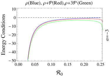
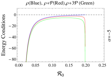
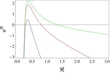
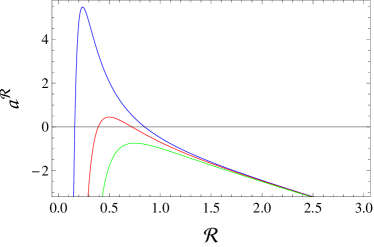
Figure 1: Energy conditions of thin-shell WHs for different values of $\alpha$.

Figure 2: Thin-shell WHs repulsive and attractive characteristics for different values of $\alpha$ as $\alpha=-4$(blue), $\alpha=-2$(red), $\alpha=1$(green) with $m=1$, $q=0.5$ (left plot) and $q=0.4$(blue), $q=0.6$(red), $q=0.8$(green) with $m=1$, $\alpha=-2$ (right plot).

The 4-acceleration radial component explains the repulsive ($a^{r}<0$) as well as the attractive ($a^{r}>0$) nature of the throat. It is found that

• For repulsive nature, an inside directed radial acceleration is needed to avoid the effect of pushed away by the WH.

• For attractive nature, an outward-directed radial acceleration is required to overcome the WH attraction.

It is noted that the radial acceleration decreases as shell radius increases as shown in Fig. 2. For highly negative values of coupling constant $\alpha$, thin-shell shows large repulsive nature as shell radius increases. We find that the repulsive behavior of the shell decreases as coupling constant approaches to positive values (left plot). It is also found that shell indicates the initially attractive behavior and then repulsive nature for different values of charge (right plot). The attractive behavior decreases as the charge of the geometry is enhanced.

IV Stability Analysis

For stability analysis, we consider static shell radius $\Re_{0}$ and expand the effective potential $\Omega(\Re)$ about $\Re_{0}$ by using Taylor series upto second order terms as follows

$$\Omega(\Re)=\Omega(\Re_{0})+\Omega^{\prime}(\Re_{0})(\Re-\Re_{0})+\frac{1}{2}\Omega^{\prime\prime}(\Re_{0})(\Re-\Re_{0})^{2}+O[(\Re-\Re_{0})^{3}].$$ (22)

It is interesting to mention that the stable and unstable geometry of the wormhole, the throat requires that the potential function and its the first derivative must be vanished at the equilibrium position, i.e., $\Omega(\Re_{0})=0=\Omega^{\prime}(\Re_{0})$. Then, it can be evaluated as:

• If the second derivative of the potential at $\Re=\Re_{0}$ is positive then it represents the stable configuration and expressed unstably structure if $\Omega^{\prime\prime}(\Re_{0})<0$.

• It is neither stable nor unstable if $\Omega^{\prime\prime}(\Re_{0})=0$.

Hence, for equilibrium configuration, Eq.(22) becomes

$$\Omega(\Re)=\frac{1}{2}\Omega^{\prime\prime}(\Re_{0})(\Re-\Re_{0})^{2}.$$ (23)

It is noted that $\rho$ and $\mathcal{P}$ obey the conservation equation given as

$$\mathcal{P}\frac{d}{d\tau}(4\pi\Re^{2})+\frac{d}{d\tau}(4\pi\Re^{2}\rho)=0.$$ (24)

The exact solution of the conservation equation depends on the choice of matter distribution which can be described through EoS. Here, we consider two types of EoS $\mathcal{P}=\mathcal{P}(\rho)$ and $\mathcal{P}=\mathcal{P}(\rho,\Re)$ 56 . The second case is more general in which surface pressure of the shell depends on both surface energy density and the throat radius. For both cases, we have $\mathcal{P}^{\prime}=\frac{d\mathcal{P}(\rho)}{d\rho}\rho^{\prime}$ and $\mathcal{P}^{\prime}=\frac{d\mathcal{P}}{d\rho}\rho^{\prime}+\frac{d\mathcal{P}}{d\Re}$, respectively. Hence, The conservation equation is yield

$$\rho^{\prime}=-\frac{2}{\Re}\{\rho+\mathcal{P}(\rho,\Re)\}.$$ (25)

For every choice of variable EoS, each solution of Eq.(25) leads to a specific form of $\Omega(\Re)$. The second derivative of effective potential at $\Re=\Re_{0}$ given as

$$\Omega^{\prime\prime}(\Re_{0}) = \frac{6q^{2}}{\Re^{4}_{0}}-16\pi^{2}\left(1+2\beta_{0}^{2}\right)(\rho^{2}_{0}+\rho_{0}\mathcal{P}_{0})+8\pi^{2}(\rho_{0}+2\mathcal{P}_{0})^{2}-\frac{4m}{\Re^{3}_{0}}$$ (26)

$$- \frac{2\alpha^{2}}{3}+16\pi^{2}\Re_{0}\rho_{0}\gamma_{0}.$$

where $\gamma_{0}=\frac{d\mathcal{P}}{d\Re}\mid_{\Re=\Re_{0}}$ and $\beta_{0}^{2}=\frac{d\mathcal{P}}{d\rho}\mid_{\Re=\Re_{0}}$. It is found that $\Omega^{\prime\prime}(\Re_{0})$ depends on EoS parameters $\gamma_{0}$ and $\beta_{0}^{2}$.

In the following, we observe the effects of barotropic and variable EoS on the stability of the developed geometry.

IV.1 Barotropic EoS

In our first case, we choose barotropic model to explore the stability of thin-shell WHs. It linearly relates the surface pressure and energy density of the matter contents given as

$$\mathcal{P}=\varpi\rho,$$ (27)

where $\varpi$ denotes the barotropic EoS parameter. By considering Eq.(27) in (25), we get

$$\rho^{\prime}(\Re)=-\frac{2}{\Re}(1+\varpi)\rho(\Re),$$ (28)

which yields

$$\rho(\Re)=\rho(\Re_{0})\left(\frac{\Re_{0}}{\Re}\right)^{2(1+\varpi)}.$$ (29)

The respective expression of the effective potential turns out to be

$$\Omega(\Re)=-4\pi^{2}\Re^{2}\rho_{0}^{2}\left(\frac{\Re_{0}}{\Re}\right)^{4(\varpi+1)}-\frac{2m}{\Re}+\frac{q^{2}}{\Re^{2}}+2\alpha q-\frac{\alpha^{2}\Re^{2}}{3}+1,$$ (30)

the first derivative with respect to throat radius $``\Re"$ at $\Re_{0}$ becomes

$$\Omega^{\prime}(\Re_{0})=\frac{4aq^{2}}{\Re_{0}^{3}}-\frac{8am}{\Re_{0}^{2}}+\frac{8\varpi\alpha q}{\Re_{0}}-\frac{4}{3}\varpi\alpha^{2}\Re_{0}+\frac{4\varpi}{\Re_{0}}-\frac{2m}{\Re_{0}^{2}}+\frac{4\alpha q}{\Re_{0}}-\frac{4\alpha^{2}\Re_{0}}{3}+\frac{2}{\Re_{0}}.$$

It is noted that $\Omega^{\prime}(\Re_{0})$ vanishes if and only if

$$\varpi=\frac{\Re_{0}\left(3m-6\alpha q\Re_{0}+2\alpha^{2}\Re_{0}^{3}-3\Re_{0}\right)}{2\left(-6m\Re_{0}+3q^{2}+6\alpha q\Re_{0}^{2}-\alpha^{2}\Re_{0}^{4}+3\Re_{0}^{2}\right)}.$$ (31)

For particular value of $\varpi=-1$, we have obtain the position of equilibrium shell radius as

$$\Re_{0}=\frac{\sqrt{9m^{2}-16\alpha q^{3}-8q^{2}}+3m}{2(2\alpha q+1)}.$$ (32)

Also, it is found that

$$\Omega^{\prime\prime}(\Re_{0}) = \frac{16\alpha^{2}\varpi^{2}}{3}+\frac{32\varpi^{2}m}{\Re_{0}^{3}}-\frac{16\varpi^{2}q^{2}}{\Re_{0}^{4}}-\frac{32\alpha\varpi^{2}q}{\Re_{0}^{2}}-\frac{16\varpi^{2}}{\Re_{0}^{2}}+\frac{4\alpha^{2}}{3}+\frac{20\alpha^{2}\varpi}{3}$$ (33)

$$+ \frac{40\varpi m}{\Re_{0}^{3}}-\frac{20\varpi q^{2}}{\Re_{0}^{4}}-\frac{40\alpha\varpi q}{\Re_{0}^{2}}-\frac{20\varpi}{\Re_{0}^{2}}+\frac{8m}{\Re_{0}^{3}}-\frac{12\alpha q}{\Re_{0}^{2}}-\frac{6}{\Re_{0}^{2}}.$$

The above equation is very useful to explore the stable characteristics of developed structure. For this purpose, it is plotted and observed different regions at equilibrium shell radius as shown in Figures 2-4. Here, it is interesting to mention that different regions mention different characteristics of the developed structure given as:

• Blue region shows neither stable nor unstable structure ($\Omega^{\prime\prime}(\Re_{0})=0$).

• Brown region represents stable geometry ($\Omega^{\prime\prime}(\Re_{0})>0$).

• Magenta region denotes unstable configuration ($\Omega^{\prime\prime}(\Re_{0})<0$).

It is noted that the developed structure expresses stable behavior if $\alpha<0$ and $q>0.5$ otherwise it represents unstable or neither stable nor unstable behavior (Fig. 3). For positive values of $\alpha$, thin-shell shows the only unstable configuration for every choice of other physical parameters. The stability of WH is increased for higher values of charged and decreased for smaller values. Similarly, the stable structure is explored along with mass, charge as well as $\alpha$ and found similar results (Figs. 3 and 5). The maximum stable regions are formed for highly negative values of $\alpha$ and higher values of charge (Fig. 5). It is found that the presence of nonlinear electrodynamics gives the possibility of stable configuration in the background of barotropic type fluid distribution. Furthermore, we plotted the second derivative of effective potential at equilibrium shell radius for these mentioned stable regions as shown in Fig. 6. It is noted that thin-shell shows stable behavior for different values of mass with negative values of $\alpha$ and stability decreases for higher values of mass. We found that the stability of WHs greatly affected by the coupling parameter and its positive as well as negative values. For higher negative values of $\alpha$, we have obtained a more stable structure as compared to less negative or positive values (right plot of Fig. 6).

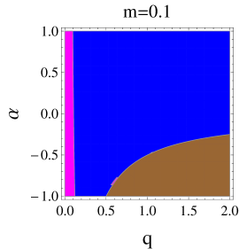
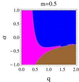
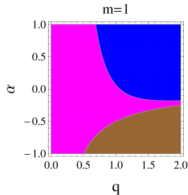
Figure 3: Region plots of $\Omega^{\prime\prime}(\Re_{0})$ verses $q$ and $\alpha$ for barotropic EoS with different values of $m$.

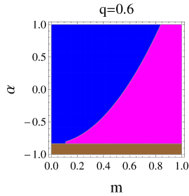
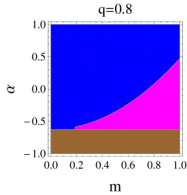
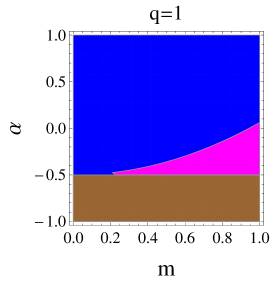
Figure 4: Region plots of $\Omega^{\prime\prime}(\Re_{0})$ verses $m$ and $\alpha$ for barotropic EoS with different values of $q$.

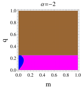
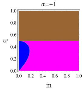
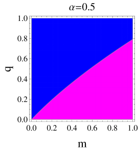
Figure 5: Region plots of $\Omega^{\prime\prime}(\Re_{0})$ verses $m$ and $q$ for barotropic EoS with different values of $\alpha$.

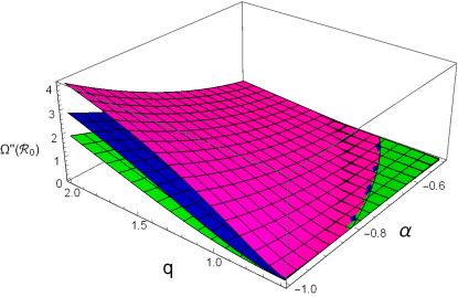
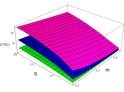
Figure 6: Stability of thin-shell WH for different values of mass as $m=0.1$(magenta) $m=0.5$(blue) $m=1$(green) (left plot) and $\alpha$ as $\alpha=-2$(magenta) $\alpha=-1.5$(blue) $\alpha=-1$(green) (right plot) in the background of barotropic type fluid distribution.

IV.2 Phantomlike Variable EoS

For second case, we consider phantomlike variable EoS to discuss the stability of thin-shell WHs 56 . Mathematically, it can be expressed as

$$\mathcal{P}=\frac{W}{\Re^{n}}\rho,$$ (34)

where $n$ is a real constant and $W$ is the EoS parameter. This equation is the generalized form of phantomlike EoS. It is reduced to phantomlike EoS for $n\rightarrow 0$. By using this EoS, the solution of conservation equation yields

$$\rho(\Re)=\rho_{0}e^{\frac{W}{n}\left(\frac{1}{\Re^{n}}-\frac{1}{\Re_{0}^{n}}\right)}\left(\frac{\Re_{0}}{\Re}\right)^{2}.$$ (35)

The corresponding effective potential turns out to be

$$\Omega(\Re)=-4\pi^{2}\Re^{2}\rho_{0}^{2}\left(\frac{\Re_{0}}{\Re}\right)^{4}e^{\frac{2W}{n}\left(\frac{1}{\Re^{n}}-\frac{1}{\Re_{0}^{n}}\right)}-\frac{2m}{\Re}+\frac{q^{2}}{\Re^{2}}+2\alpha q-\frac{\alpha^{2}\Re^{2}}{3}+1.$$ (36)

It is noted that effective potential vanishes at $\Re=\Re_{0}$ and its first derivative is given as

$$\Omega^{\prime}(\Re_{0})=\frac{1}{3}\Re_{0}^{-n-3}\left(24\pi^{2}\rho_{0}^{2}\Re_{0}^{4}\left(W+\Re_{0}^{n}\right)-2\Re_{0}^{n}\left(-3m\Re_{0}+3q^{2}+\alpha^{2}\Re_{0}^{4}\right)\right),$$ (37)

By taking $\Omega^{\prime}(\Re_{0})=0$, we obtain

$$W=\frac{-3m\Re_{0}^{n+1}+6\alpha q\Re_{0}^{n+2}-2\alpha^{2}\Re_{0}^{n+4}+3\Re_{0}^{n+2}}{-3\left(\Re_{0}(\Re_{0}-2m)+q^{2}\right)-6\alpha q\Re_{0}^{2}+\alpha^{2}\Re_{0}^{4}}.$$ (38)

Hence, we have

$$\Omega^{\prime\prime}(\Re_{0}) = -\frac{2}{3}\Re_{0}^{-2(n+2)}\left(\left(2W^{2}+W(n+5)\Re_{0}^{n}+3\Re_{0}^{2n}\right)\left(3q^{2}+6\alpha q\Re_{0}^{2}\right.\right.$$ (39)

$$- \left.\left.\Re_{0}\left(6m+\alpha^{2}\Re_{0}^{3}-3\Re_{0}\right)\right)+\Re_{0}^{2n}\left(6m\Re_{0}-9q^{2}+\alpha^{2}\Re_{0}^{4}\right)\right).$$

The stability of thin-shell filled with phantomlike variable EoS is analyzed graphically. It is noted that the stable regions exist if and only if both $n$ and $\alpha$ are positive or negative (Figs. 7-9). If $\alpha<0$, then $n$ must be negative for stability with every value of physical parameters. Fig. 9 indicates that stable regions occurs when $\alpha>0$ and $n>5$. Hence, for such type of matter contents, there must exist a possibility of stable regions at which $\Omega^{\prime\prime}(\Re_{0})>0$ for specific values of mass and charge. For large stable regions, it is noted that both $\alpha$ and $n$ must be negative. We also noted that stability of the shell increases for highly negative values of $n$ and $\alpha$ as shown in left and right plots of Fig. 10.

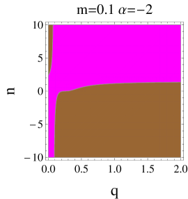
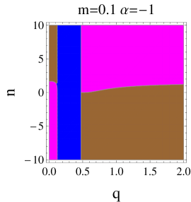
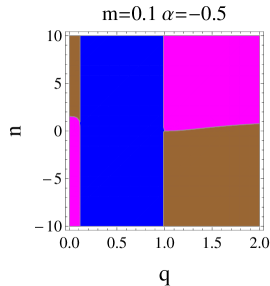
Figure 7: Region plots of $\Omega^{\prime\prime}(\Re_{0})$ verses $q$ and $n$ for phantomlike variable EoS with different values of $\alpha$.

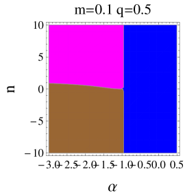
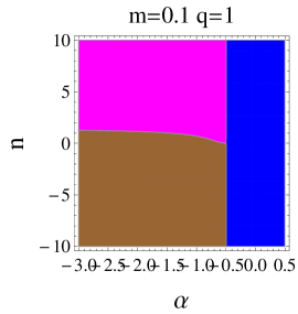
Figure 8: Region plots of $\Omega^{\prime\prime}(\Re_{0})$ verses $\alpha$ and $n$ for phantomlike variable EoS with different values of $q$.

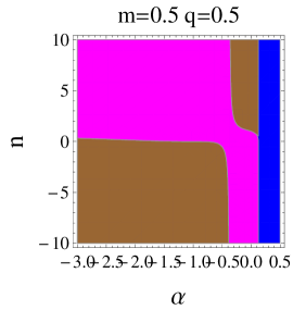
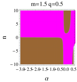
Figure 9: Region plots of $\Omega^{\prime\prime}(\Re_{0})$ verses $\alpha$ and $n$ for phantomlike variable EoS with different values of $m$.

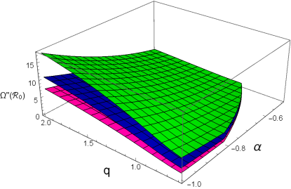
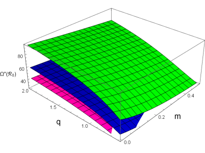
Figure 10: Stability of thin-shell WH with phantomlike EoS for different values of $n$ as $n=-1$(magenta) $n=-2$(blue) $n=-5$(green) with $m=0.1$ (left plot) and $\alpha=-2$ (right plot).

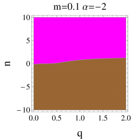
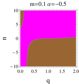
Figure 11: Region plots of $\Omega^{\prime\prime}(\Re_{0})$ verses $q$ and $n$ for Chaplygin variable EoS with different values of $\alpha$.

IV.3 Chaplygin Variable EoS

In the last case, we consider Chaplygin variable EoS written as 56

$$\mathcal{P}=\frac{1}{\Re^{n}}\frac{C}{\rho},$$ (40)

where $C$ is the EoS parameter. This reduces to Chaplygin EoS for $n\rightarrow 0$. The solution of conservation equation in terms of surface energy density is

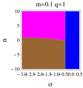
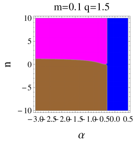
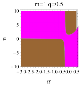
Figure 12: Region plots of $\Omega^{\prime\prime}(\Re_{0})$ verses $\alpha$ and $n$ for Chaplygin variable EoS with different values of $q$.

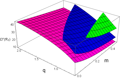
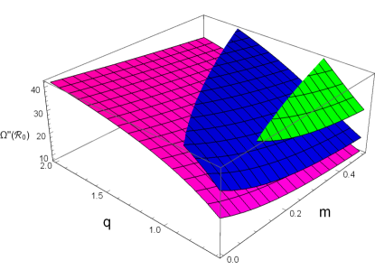
Figure 13: Region plots of $\Omega^{\prime\prime}(\Re_{0})$ verses $\alpha$ and $n$ for Chaplygin variable EoS with different values of $m$.

Figure 14: Stability of thin-shell WH with Chaplygin gas for different values of $n$ as $n=-1$(magenta) $n=-2$(blue) $n=-5$(green) with $m=0.1$ (left plot) and $\alpha=-2$ (right plot).

$$\rho^{2}(\Re)=\frac{4C\left(\Re^{4}\Re_{0}^{n}-\Re^{n}\Re_{0}^{4}\right)+\rho_{0}^{2}\Re_{0}^{n+4}\Re^{n}(n-4)}{(n-4)\Re^{n+4}\Re_{0}^{n}}.$$ (41)

We obtain the respective potential function for such type of matter distribution and noted that $\Omega(\Re_{0})=0$. Also, we calculate $\Omega^{\prime}(\Re)$ and taking $\Omega^{\prime}(\Re_{0})=0$ so that

$$C=-\frac{m\Re_{0}^{n-3}}{8\pi^{2}}+\frac{q^{2}\Re_{0}^{n-4}}{8\pi^{2}}+\frac{\alpha^{2}\Re_{0}^{n}}{24\pi^{2}}-\frac{1}{2}\rho_{0}^{2}\Re_{0}^{n}.$$ (42)

Second derivative of potential function with respect to shell radius at $\Re=\Re_{0}$ written as

$$\Omega^{\prime\prime}(\Re_{0}) = -\frac{2mn}{\Re_{0}^{3}}+\frac{6m}{\Re_{0}^{3}}-\frac{1}{3}4\alpha^{2}n+\frac{4\alpha nq}{\Re_{0}^{2}}+\frac{2n}{\Re_{0}^{2}}-\frac{8\alpha q}{\Re_{0}^{2}}-\frac{4}{\Re_{0}^{2}}.$$ (43)

For Chaplygin variable EoS, the maximum stable regions are obtained only if both $n$ and $\alpha$ are negative as shown in Figs. 11-13. It is found that stable regions increase for negative values of $\alpha$ and decreases as $\alpha$ approaches positive values. Higher values of charge also enhance the stable regions. Similarly, we have obtained that the stability of the developed structure is maximum as $n$ as well as $\alpha$ have maximum negative values and stability decreases as $\alpha$ or $n$ approaches zero or positive values (Fig. 14).

V Concluding Remarks

This paper has explored the effects of nonlinear electrodynamics on the stable configuration of thin-shell WHs. For this purpose, we have constructed WH geometry through the matching of two equivalent copies of RN BH with nonlinear electrodynamics. The components of matter filled at thin-shell are found by using a reduced form of Einstein field equations known as Lanczos equations. The developed structure is physically acceptable for the WH geometry as null and weak energy conditions are violated (Fig. 1). It is noted that the attractive and repulsive nature of the WH throat is greatly affected by the coupling parameter $\alpha$ (Fig. 2). We have analyzed the stability of the developed structure by using radial perturbation with three different types of matter distributions, i.e., barotropic, phantomlike variable, and Chaplygin variable EoS.

Firstly, we have considered barotropic type fluid distribution and analyzed the stable configuration graphically (Figs. 3-6). It is worthwhile to mention that the developed structure shows stable regions for barotropic EoS if $\alpha<0$ (Figs. 3-5). It is noted that WH geometry developed from Schwarzschild and RN BHs express unstable behavior for every choice of physical parameter for barotropic EoS 56 ; 57 . Hence, the presence of nonlinear electrodynamics provides stability of WH geometry for barotropic EoS. It is found that stable regions increase by an increasing charge of the geometry with negative values of coupling parameters. These results also supported the final results of published articles 56 -59 .

Secondly, we have interested to observe the stability of thin-shell filled with phantomlike variable EoS (Figs. 7-10). It is found that stable regions must exist for every choice of the physical parameter if $n<0$ and $\alpha<0$ (Figs. 7-9). There is also a possibility for a stable structure if both $\alpha$ and $n$ are positive. It is also noted that the developed structure is more stable in the presence of nonlinear electrodynamics. As thin-shell, WHs developed from Schwarzschild, RN, Bardeen, and Bardeen-de Sitter BHs have less stable configurations for some specific values of the physical parameter while RN BH with nonlinear electrodynamics is more suitable for the construction of stable thin-shell WH 56 -59 .

Finally, we have analyzed the effects of Chaplygin variable EoS on the stability of the developed structure (Figs. 11-14). It is found that there exist more stable regions if both $\alpha$ and $n$ have the same sign (Figs. 11-13). It is also noted that the stability of the geometry increases by an increasing charge of the geometry. The stable configuration decreases as $\alpha$ and $n$ lead to positive values and increases as $\alpha$ and $n$ approach large negative values (Fig. 14).

It is concluded that thin-shell WH with nonlinear electrodynamics expresses more stable regions as compared to WH geometry developed from Schwarzschild, RN, Bardeen and Bardeen-de Sitter BHs 56 -59 .

References

- (1) Born, M. and Infeld, L., On the quantum theory of the electromagnetic field, Proc. Roy. Soc. Lond. A 143(1934)410; ibid, Foundations of the new field theory, 144(1934)425.
- (2) Fradkin, E.S. and Tseytlin, A., Non-linear electrodynamics from quantized strings, Phys. Lett. B 163(1985)123.
- (3) Novello, M., Perez Bergliaffa, S.E. and Salim, J., Nonlinear electrodynamics and the acceleration of the universe, Phys. Rev. D 69(2004)127301; Dyadichev, V.V., Galtsov, D.V. and Moniz, P.V., New Features about Chaos in Bianchi I non-Abelian Born-Infeld cosmology, AIP Conf. Proc. 861(2006)312.
- (4) Aharony, O., A brief review of “little string theories”, Class. Quantum Grav. 17(2000)929.
- (5) Ayn-Beato, E., Garca, A., Regular black hole in general relativity coupled to nonlinear electrodynamics, Phys. Rev. Lett. 80(1998)5056; New regular black hole solution from nonlinear electrodynamics, Phys. Lett. B 464(1999)25; Non-singular charged black hole solution for non-linear source, Gen. Rel. Grav. 31(1999)629; Four-parametric regular black hole solution, Gen. Rel. Grav. 37(2005)635.
- (6) Mazharimousavi, S.H. and Halilsoy, M., Lovelock black holes with a power-Yang-Mills source, Phys. Lett. B 681(2009)190.
- (7) Bronnikov, K.A., Regular magnetic black holes and monopoles from nonlinear electrodynamics, Phys. Rev. D 63(2001)044005.
- (8) Dehghani, M.H., Bostani, N. and Hendi, S.H., Magnetic branes in third order Lovelock-Born-Infeld gravity, Phys. Rev. D 78(2008)064031.
- (9) Dehghani, M.H., Sheykhi, A. and Hendi, S.H., Magnetic strings in Einstein-Born-Infeld-dilaton gravity, Phys. Lett. B 659(2008)476.
- (10) Dehghani, M.H. and Hendi, S.H., thermodynamics of rotating black branes in Gauss-Bonnet-Born-Infled gravity, Int. J. Mod. Phys. D 16(2007)1829; Wormhole solutions in Gauss-Bonnet-Born-Infeld gravity, Gen. Rel. Grav. 41(2009)1853.
- (11) Aiello, M., Ferraro, R. and Giribet, G., Exact solutions of Lovelock-Born-Infeld black holes, Phys. Rev. D 70(2004)104014.
- (12) Dehghani, M.H., Alinejadi, N. and Hendi, S.H., Topological black holes in Lovelock-Born-Infeld gravity, Phys. Rev. D 77(2008)104025.
- (13) Ayn-Beato, E., Garca, A., The Bardeen model as a nonlinear magnetic monopole, Phys. Lett. B 493(2000)149.
- (14) Johannsen, T., Regular black hole metric with three constants of motion, Phys. Rev. D 88(2013)044002.
- (15) Dymnikova, I. and Galaktionov, E., From a locality-principle for new physics to image features of regular spinning black holes with disks, Class. Quantum Grav. 32(2015)165015.
- (16) Bronnikov, K.A., Baleevskikh, K.A. and Skvortsova, M.V., Multihorizon spherically symmetric spacetimes with several scales of vacuum energy, Class. Quantum Grav. 29(2012)095025; Wormholes with fluid sources: A no-go theorem and new examples, Phys. Rev. D 96(2017)124039.
- (17) Yu, S. and Gao, C., Exact black hole solutions with nonlinear electrodynamic field, Int. J. Mod. Phys. D 29(2020)2050032.
- (18) Morris, M.S. and Thorne, K.S., Wormholes in spacetime and their use for interstellar travel: A tool for teaching general relativity, Am. J. Phys. 56(1988)395.
- (19) S. Capozziello et al., Wormholes supported by hybrid metric-Palatini gravity, Phys. Rev. D 86 (2012) 127504.
- (20) S. Capozziello et al., Constructing superconductors by graphene Chern-Simons wormholes, Ann. Phys. 390 (2018) 303.
- (21) S. Capozziello, R. Pincak and E. Bartos, Chern-Simons current of left and right chiral superspace in graphene wormhole, Symmetry 12 (2020) 774.
- (22) S. Capozziello and M. Francaviglia, Extended theories of gravity and their cosmological and astrophysical applications, Gen. Relativ. Gravit. 40 (2008) 357.
- (23) S. Capozziello et al., Cosmological viability of gravity as an ideal fluid and its compatibility with a matter dominated phase, Phys. Lett. B 639 (2006) 135.
- (24) S. Capozziello, V. F. Cardone and A. Troisi, Reconciling dark energy models with theories, Phys. Rev. D 71 (2005) 043503.
- (25) S. Capozziello, A. Stabile and A. Troisi, Spherically symmetric solutions in gravity via Noether symmetry approach, Class. Quantum Grav. 24 (2007) 2153.
- (26) M. Sharif, F. Javed, Stability of charged thin-shell gravastars with quintessence, Eur. Phys. J. C 81(2021)47; Mechanical stability of a class of regular thin-shell wormholes, Mod. Phys. Lett. A 39(2020)2050309; Stability and dynamics of regular thin-shell gravastars, J. Exp. Theor. Phys. 132(2021)381; Stability of charged thin-shell wormholes with Weyl corrections, Astronomy Reports 65(2021)353.
- (27) S. Capozziello et al., Hydrostatic equilibrium and stellar structure in gravity, Phys. Rev. 83 (2011) 064004
- (28) V. D. Falco, E. Battista, S. Capozziello and M. D. Laurentis, General relativistic Poynting-Robertson effect to diagnose wormholes existence: Static and spherically symmetric case, Phys. Rev. D 101 (2020) 104037.
- (29) V. D. Falco, E. Battista, S. Capozziello and M. D. Laurentis, Testing wormhole solutions in extended gravity through the Poynting-Robertson effect, Phys. Rev. D 103 (2021) 044007.
- (30) V. D. Falco, E. Battista, S. Capozziello and M. D. Laurentis, Reconstructing wormhole solutions in curvature based extended theories of gravity, Eur. Phys. J. C 81 (2021) 157.
- (31) M. Sharif, F. Javed, Stable bounded excursion gravastars with regular black holes, Astrophys Space. Sci. 366(2021)103; Dynamics of the scalar shell in higher dimensions, Ann. Phys. 416(2020)168146.
- (32) V. D. Falco, M. D. Laurentis and S. Capozziello, Epicyclic frequencies in static and spherically symmetric wormhole geometries, Phys. Rev. D 104(2) (2021) 024053.
- (33) Visser, M., Traversable wormholes: Some simple examples, Phys. Rev. D 39(1989)3182.
- (34) Visser, M., Traversable wormholes from surgically modified Schwarzschild spacetimes, Nucl. Phys. B 328(1989)203.
- (35) Israel, W., Singular hypersurfaces and thin shells in general relativity, Nuovo Cimento B 44(1966)1.
- (36) Poisson, E. and Visser, M., Thin-shell wormholes: Linearization stability, Phys. Rev. D 52(1995)7318.
- (37) Kim, S.W. and Lee, H., Exact solutions of a charged wormhole, Phys. Rev. D 63(2001)064014.
- (38) Eiroa, E.F. and Romero, G.E., Thin-Shell Wormholes in Einstein and Einstein-Gauss-Bonnet Theories of Gravity, Gen. Relativ. Gravit. 36(2004)651.
- (39) Eiroa, E.F. and Simeone, C., Stability of Chaplygin gas thin-shell wormholes, Phys. Rev. D 76(2007)024021.
- (40) Mazharimousavi, S.H., Halilsoy, M. and Amirabi, Z., Stability of thin-shell wormholes supported by normal matter in Einstein-Maxwell-Gauss-Bonnet gravity, Phys. Rev. D 81(2010)104002.
- (41) Sharif, M. and Azam, M., Stability analysis of thin-shell wormholes from charged black string, J. Phys. Soc. Jp. 81(2012)124006.
- (42) Amirabi, Z., Halilsoy, M. and Habib Mazharimousavi, S., Effect of the Gauss-Bonnet parameter in the stability of thin-shell wormholes, Phys. Rev. D 88(2013)124023.
- (43) Sharif, M. and Azam, M., Mechanical stability of cylindrical thin-shell wormholes, Eur. Phys. J. C 73(2013)2407.
- (44) Forghani, S.D., Habib Mazharimousavi, S. and Halilsoy, M., Asymmetric thin-shell wormholes, Eur. Phys. J. C 78(2018)469.
- (45) M. Sharif, F. Javed, Collapse and expansion of scalar thin-shell for a class of black holes, Int. J. Mod. Phys. D 28(2019)1950046; Dynamical evolution of scalar field thin-shell for rotating regular black holes, Ann. Phys. 407(2019)198; Stability of Einstein-power-Maxwell (2+1)-dimensional wormholes, Chin. J. Phys. 61(2019)262; Dynamics of scalar shell for rotating and charged rotating BTZ black holes, Mod. Phys. Lett. A 35(2019)1950350.
- (46) M. Sharif, F. Javed, Stability of charged rotating (2 + 1)-dimensional wormholes, Int. J. Mod. Phys. D 29(2020)2050007; Stability of gravastars with exterior regular black holes, Ann. Phys. 415(2020)168124.
- (47) Varela, V., Note on linearized stability of Schwarzschild thin-shell wormholes with variable equations of state, Phys. Rev. D 92(2015)044002.
- (48) Eid, A., Charged thin shell wormholes with variable equations of state, Adv. Stud. Theo. Phys. 9(2015)503.
- (49) Sharif, M. and Javed, F., On the stability of bardeen thin-shell wormholes, Gen. Relativ. Gravit. 48(2016)158; Linearized stability of Bardeen anti-de Sitter wormholes, Astrophys Space. Sci. 364(2019)179.
- (50) Sharif, M. and Javed, F., Stability of charged thin-shell and thin-shell wormholes: a comparison, Phys. Scr. 96(2021)055003.
- (51) F. Javed, G. Mustafa, A. Övgün and M. F. Shamir, Epicyclic frequencies and stability of thin shell around the traversable phantom wormholes in Rastall gravity, Eur. Phys. J. Plus 137 (2022) 61.
- (52) G. Mustafa, M. Ahmad, A. Övgün, M. Farasat Shamir and I. Hussain, Traversable wormholes in the extended teleparallel theory of gravity with matter coupling, Fortschr. Phys., Prog. Phys. 69 (2021) 2100048.
- (53) G. Mustafa, X. Gao, and Faisal Javed, Twin Peak Quasi-Periodic Oscillations and Stability via Thin-Shell Formalism of Traversable Wormholes in Symmetric Teleparallel Gravity, Fortschr. Phys. 2022, 2200053