Towards the phase diagram of cold and dense heavy QCD

Abstract

The thermodynamics of QCD with sufficiently heavy dynamical quarks can be described by a three-dimensional Polyakov loop effective theory, obtained after a truncated character and hopping expansion. We investigate the resulting phase diagram for low temperatures by mean field methods. Taking into account chemical potentials for both baryon number and isospin, we obtain clear signals for a liquid-gas type transition to baryon matter at $\mu_{I}=0$ and a Bose-Einstein condensation transition at $\mu_{B}=0$, as well as for their connection when both chemical potentials are non-zero.

1 Introduction

The QCD phase structure in the $(T,\mu_{B})$ plane is important to understand many physical phenomena for various disciplines in modern physics. The interest in neutron stars and their mergers moreover motivates studies of non-vanishing isospin chemical potential $\mu_{I}\neq 0$, and in particular the mixed situation with both $\mu_{B},\mu_{I}\neq 0$. While ordinary Monte Carlo simulations are possible for $(\mu_{B}=0,\mu_{I}\neq 0)$, cf. [1] and references therein, a strong sign problem causes their breakdown whenever the baryon chemical potential $\mu_{B}\neq 0$. Most methods to circumvent the obstacle introduce further approximations, and are therefore restricted to the region with $\mu_{B}/T\leq 3$ (see for example Refs. [2, 3, 4]).

Our approach is to study $3D$ effective Polyakov loop lattice theories, which are obtained from Wilson’s lattice QCD when integrating over all spatial links after a truncated strong coupling and hopping parameter expansion, and describe QCD with very heavy quarks [5]. Here we investigate the phase diagram of the simplest of these effective theories with a mean field approach, and compare with previous solutions obtained by series expansions or Monte Carlo simulations. After successful tests with the finite temperature deconfinement transition we consider $T\rightarrow 0$, where we identify both the onset transition to cold baryon matter at $\mu_{B}\approx m_{B},\mu_{I}=0$, as well as the transition to a pion condensate at $\mu_{B}=0,\mu_{I}=m_{\pi}/2$. Finally, we switch on both chemical potentials and follow the critical lines into the $(\mu_{B},\mu_{I})$-plane. We find them to connect in a branching point, where the vacuum, baryon and pion phases meet.

2 The effective theory

In this section we summarise the main features of the effective theory to be analysed below, for details see [6, 5]. Starting point is the path integral

$$Z =\int\quantity[\differential U_{\mu}]~{}\Big{(}\prod^{N_{f}}_{f=1}\det Q_{f}\quantity[U_{\mu}]\Big{)}e^{-S_{g}\quantity[U_{\mu}]}=\int\quantity[\differential U_{0}]e^{-S_{\text{eff}}[U_{0}]},$$ (1)

with

$$-S_{\text{eff}}[U_{0}]\equiv\ln\int\quantity[\differential U_{i}]\quantity[\Big{(}\prod^{N_{f}}_{f=1}\det Q_{f}\quantity[U_{\mu}]\Big{)}~{}e^{-S_{g}[U_{\mu}]}].$$ (2)

An approximation of the effective action Eq. (2) can be obtained after a truncated expansion of the gauge action in terms of the fundamental character coefficients $u(\beta)$ and a hopping expansion of the fermion determinants in terms of the hopping parameters $\kappa_{f}$ [7],

$$u(\beta)=\beta/18+\beta^{2}/216+\ldots,\quad\kappa_{f}=(2am_{f}+8)^{-1},$$ (3)

followed by analytic integrating over the spatial gauge links. Because of the hopping expansion, the resulting effective theory is only valid for large bare quark masses $m_{f}$. Here we specialise to mass-degenerate quarks, for which $m_{f}=m,\kappa_{f}=\kappa$ for all flavours $f$. The remaining dependence on the temporal gauge links is in terms of untraced Wilson lines, $W(\mathbf{x})=\prod^{N_{\tau}}_{\tau=1}U_{0}\quantity(\mathbf{x},\tau)$, and Polyakov loops, $L\quantity(\mathbf{x})=\Tr W(\mathbf{x})$. The result after these steps can be written as,

$$Z \approx\int DW\underbrace{\prod_{\expectationvalue{\mathbf{x},\mathbf{y}}}\quantity[1+\lambda_{1}\quantity(L^{\dagger}_{\mathbf{x}}L_{\mathbf{y}}+L_{\mathbf{x}}L^{\dagger}_{\mathbf{y}})]}_{\text{pure gauge}}$$ (4)

$$\times\underbrace{\prod_{\mathbf{x}}\prod^{N_{f}}_{f=1}\quantity(1+h_{1f}L_{\mathbf{x}}+h_{1f}^{2}L^{\dagger}_{\mathbf{x}}+h_{1f}^{3})^{2}~{}\quantity(1+\overline{h}_{1f}L^{\dagger}_{\mathbf{x}}+\overline{h}_{1f}^{2}L_{\mathbf{x}}+\overline{h}_{1f}^{3})^{2}}_{\text{static}}$$

$$\times\prod_{\expectationvalue{\mathbf{x},\mathbf{y}}}\underbrace{\quantity(1-2h_{2}\sum^{N_{f}}_{f=1}\quantity[W^{f}_{11}\quantity(\mathbf{x})-\overline{W}^{f}_{11}\quantity(\mathbf{x})]\quantity[W^{f}_{11}\quantity(\mathbf{y})-\overline{W}^{f}_{11}\quantity(\mathbf{y})])}_{\text{kinetic}}$$

with the effective couplings [6]

$$\lambda_{1} = u^{N_{\tau}}\exp\quantity[N_{\tau}\quantity(4u^{4}+12u^{5}-14u^{6}-16u^{7}+\frac{295}{2}u^{8}+\frac{1851}{10}u^{9}+\frac{1055797}{5120}u^{10})]$$

$$h_{1f} = 2\kappa\exp\quantity[N_{\tau}a\mu_{f}]\exp\quantity[6N_{\tau}\kappa^{2}u\quantity(\frac{1-u^{N_{\tau}-1}}{1-u}+4u^{4}-12\kappa^{2}+9\kappa^{2}u+4\kappa^{2}u^{2}-4\kappa^{4})]$$

$$\overline{h}_{1f} = 2\kappa\exp\quantity[-N_{\tau}a\mu_{f}]\exp\quantity[6N_{\tau}\kappa^{2}u\quantity(\frac{1-u^{N_{\tau}-1}}{1-u}+4u^{4}-12\kappa^{2}+9\kappa^{2}u+4\kappa^{2}u^{2}-4\kappa^{4})]$$

$$h_{2} = \frac{N_{\tau}\kappa^{2}}{N_{c}}\quantity(1+2\frac{u-u^{N_{\tau}}}{1-u}+8u^{5}+16\kappa^{3}u^{4}).$$

The expressions appearing in the third line in Eq. (4) are defined as

$$W^{f}_{nm}\quantity(\mathbf{x})=\Tr\frac{\quantity(h_{1f}W_{\mathbf{x}})^{m}}{\quantity(\mathbb{I}+h_{1f}W_{\mathbf{x}})^{n}},\quad\overline{W}^{f}_{nm}\quantity(\mathbf{x})=\Tr\frac{\quantity(\overline{h}_{1f}W^{\dagger}_{\mathbf{x}})^{m}}{\quantity(\mathbb{I}+\overline{h}_{1f}W^{\dagger}_{\mathbf{x}})^{n}}.$$ (5)

The effective theory in Eq. (4) is structured as follows: the first line represents the pure gauge contribution, the second line contains the static determinant, and the last line is the leading order of the kinetic quark determinant. All contributions can be expressed fully in terms of Polyakov loops, if desired. An important feature of this effective theory is that it has a much weaker sign problem than full QCD and can therefore be simulated using reweighting techniques or complex Langevin methods [5, 8]. Moreover, it can also be treated by analytic linked-cluster expansion methods in the effective couplings [9, 10, 11].

3 Mean field analysis of the effective theory

Since the effective theory resembles a spin model, it is natural to also consider mean field methods as a short cut to a first evaluation and to get an impression of the overall phase structure. We proceed in analogy to early investigations of similar models [12, 13]. The basic idea is to consider fluctuations of the Polyakov loop around its mean field value, $L_{\mathbf{x}}=\overline{L}+\delta L_{\mathbf{x}}$ and $L^{*}_{\mathbf{x}}=\overline{L}+\delta L^{*}_{\mathbf{x}}$, and to expand the effective action up to linear order in the fluctuations,

$$S_{\text{eff}}\quantity[L]\approx S_{\text{eff}}\quantity[\overline{L}]+\sum_{\mathbf{x}}\quantity(\partialderivative{S_{\text{eff}}}{L}\bigg{|}_{\overline{L}}\delta L_{\mathbf{x}}+\partialderivative{S_{\text{eff}}}{L^{*}}\bigg{|}_{\overline{L}^{*}}\delta L^{*}_{\mathbf{x}})+\dots\;.$$

Inserting this mean field approximation, the path integral for the effective theory simplifies to

$$Z_{\mathrm{mf}}=f\quantity(\overline{L})\quantity[\int\differential W\exp\quantity{-\partialderivative{S_{\text{eff}}}{\overline{L}}L-\partialderivative{S_{\text{eff}}}{\overline{L}^{*}}L^{*}}]^{V}.$$ (6)

The expression $f\quantity(\overline{L})$ represents the saddle point contribution to the path integral and reads

$$f\quantity(\overline{L})=\exp\quantity[-S_{\text{eff}}[\overline{L}]+\partialderivative{S_{\text{eff}}}{\overline{L}}\overline{L}+\partialderivative{S_{\text{eff}}}{\overline{L}^{*}}\overline{L}^{*}]\;.$$ (7)

The remaining integration in Eq. (6) is reduced to one-site integrals, which can be done after expanding down the exponential, as shown in the example below. After that we have an explicit formula to calculate the free energy in the mean field approximation,

$$F_{\mathrm{mf}}=-\ln Z_{\mathrm{mf}}\;.$$ (8)

4 A test case: deconfinement transition in pure gauge theory

To illustrate our concrete calculations, we list the resulting expressions for the effective theory representing finite temperature Yang-Mills theory, i.e., the partition function Eq. (4) reduced to its first line with one effective coupling only. This will also provide a test of our mean field procedure. For the linearised corresponding effective action we have

$$-S_{\text{eff}}[L]\approx d\sum_{\mathbf{x}}\quantity[\ln\quantity(1+2\lambda_{1}\absolutevalue{\overline{L}}^{2})+\frac{2d\lambda_{1}}{\quantity(1+2\lambda_{1}\absolutevalue{\overline{L}}^{2})}\quantity(\bar{L}^{*}\delta L_{\mathbf{x}}+\bar{L}\delta L^{*}_{\mathbf{x}})]\;,$$ (9)

where $d=3$ denotes the number of space dimensions. The saddle point contribution then is

$$f(\overline{L})=\exp\quantity[Vd\ln\quantity(1+2\lambda_{1}\absolutevalue{\overline{L}}^{2})+\frac{2Vd}{\quantity(1+2\lambda_{1}\absolutevalue{\overline{L}}^{2})}]$$ (10)

and the partition function in the mean field approximation

$$Z_{\mathrm{mf}} =f(\overline{L})\quantity[\int\differential W\exp\left\{\frac{2d\lambda_{1}\overline{L}^{*}}{1+2\lambda_{1}\absolutevalue{\overline{L}}^{2}}~{}L+\frac{2d\lambda_{1}\overline{L}}{1+2\lambda_{1}\absolutevalue{\overline{L}}^{2}}~{}L^{*}\right\}]^{V}$$

$$=f(\overline{L})\quantity[\sum_{n,m}\frac{\quantity(z_{1})^{n}\quantity(z_{2})^{m}}{n!m!}\int\differential W~{}L^{n}\quantity(L^{*})^{m}]^{V}$$ (11)

with

$$z_{1}\equiv\frac{2d\lambda_{1}\overline{L}^{*}}{1+2\lambda_{1}\absolutevalue{\overline{L}}^{2}}\;,\quad z_{2}\equiv\frac{2d\lambda_{1}\overline{L}}{1+2\lambda_{1}\absolutevalue{\overline{L}}^{2}}\;.$$ (12)

To proceed we need to evaluate the Polyakov loop integrals, for which we we use the formula [14]

$$\int\differential W~{}L^{n}\quantity(L^{*})^{m}=\sum^{\lfloor\frac{n}{3}\rfloor}_{j=\max\quantity(0,\frac{n-m}{3})}\frac{T(n-m)~{}2n!~{}m!~{}\binom{3\quantity(n-j-\frac{n-m}{3}+1)}{n-3j}\binom{2j-\frac{n-m}{3}}{j}}{\quantity(n-j-\frac{n-m}{3}+1)!\quantity(n-j-\frac{n-m}{3}+2)!\quantity(2j-\frac{n-m}{3})!}\;,$$ (13)

with binomial coefficients and the triality function $T(n)=1$ if $n\;\mbox{mod}\;3=0$, and $T(n)=0$ otherwise.

It is well known from lattice simulations that 4d $SU(3)$ pure gauge theory at finite temperature features a first-order deconfinement transition due to spontaneous center symmetry breaking, which is faithfully reproduced by the 3d effective theory [6]. In Fig. 1 we display the mean field free energy density as a function of the real part of the Polyakov loop. For decreasing effective coupling we indeed observe a non-trivial second minimum to form at non-vanishing expectation values, which triggers the center symmetry breaking transition in the effective theory. Since there is a hill between the minima, this is a first-order transition. The critical coupling for the transition is the value where the two minima are degenerate, which happens at $\lambda_{1c}=0.152$. This is to be compared with a Monte Carlo simulation of the 3d effective theory, which gives $\lambda_{1c}=0.188$ [6]. We conclude that the mean field treatment reproduces the correct order of the deconfinement phase transition, and the predicted critical coupling is within a reasonable 20% of the true answer. For an extension of the deconfinement transition to the situation with dynamical quarks, which is also reproduced, as well as further refinements of the mean field approach, see [15].

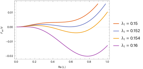
Figure 1: Pure Gauge Case: Mean-Field free energy $\mathcal{F_{\text{mf}}}$ as a function of the expectation value of the Polyalov-Loop $\expectationvalue{L}$, with different values around the critical values of $\lambda_{1}$.

5 Phase structure for zero temperature and finite chemical potentials

After this successful test, we proceed to our case of interest, namely QCD with dynamical quarks at low temperatures with non-vanishing chemical potentials. Now Eq. (4) will be considered with all contribution up to $\kappa^{2}$ and $N_{f}=2$. For finite baryon chemical potential, $\mu_{u}=\mu_{d}=\mu_{B}/3$, the effective theory has a sign problem, which however is much milder than the original one. It has been demonstrated that the effective theory can be simulated with a choice of different algorithms. As expected, the theory displays an onset transition to a medium with net baryon density at $\mu_{B}\approx m_{B}$ [16, 8]. Like the deconfinement transition, our mean field treatment reproduces this baryon onset to be first-order for sufficiently large $N_{\tau}$, i.e. low temperatures, by our mean field treatment.

Here, we investigate for the first time how the effective theory behaves when isospin chemical potenital is introduced, $\mu_{I}=\quantity(\mu_{u}-\mu_{d})/2$. In Fig. 2 we display the mean field free energy density for the QCD lattice parameters $\beta=5.7,\kappa=0.0004$ and $N_{\tau}=10000$. Upon increasing isospin chemical potential, we observe a flattening of the potential well and the formation of a minimum for a non-vanishing value of the Polyakov loop expectation value. In contrast to the previous transitions, there is no hill in the free energy density separating minima, but instead a critical value of the chemical potential where the curvature vanishes. This feature predicts the phase transition to be second order. Once again, this result is fully compatible with what is found in simulations of full QCD at the physical point with an isospin chemical potential [1].

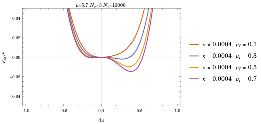
Figure 2: Variation of the mean field free energy density with the isospin chemical potential, lattice parameters: $\beta=5.7$ and $N_{\tau}=10000$

In contrast to any other method, our effective theory now permits us to consider non-vanishing baryon and isospin chemical potential at the same time, and to follow what happens to the observed first-order baryon onset and second-order isospin condensation transitions, respectively. That is, we keep $N_{\tau}=10000$ fixed and identify the critical combinations $(\mu_{B}^{c},\mu_{I}^{c})$ by either coexistence of two degenerate minima (first order) or a vanishing curvature (second order) in the mean field free energy density. The result is shown in Fig. 3, where the chemical potentials are given in terms of the baryon and pion masses, which are here crudely approximated by their leading order values in the hopping expansion, $am_{B}=-3\ln(2\kappa),\;am_{\pi}=-2\ln(2\kappa)$.

In Fig. 3 we observe both transitions to curve towards each other, and to join in a special point, where the order of the transition changes. That the baryon and pion onset transitions must connect somewhere is also to be expected before an explicit calculation. The region below the transition line represents vacuum, whereas above it the ground state of the system is either baryon matter or a Bose-Einstein condensate of pions. In both of the latter cases there is a medium whose rest frame breaks Lorentz symmetry. Thus a true phase transition must exist, independent of the direction in the plane of chemical potentials. Similarly, a Bose-Einstein condensate $\langle m_{\pi}^{\pm}\rangle\neq 0$ and a non-vanishing baryon expectation value $\langle n_{B}\rangle\neq 0$ are distinguished by quantum numbers pertaining to different symmetries. Consequently, baryon matter must be separated from pion matter by a true phase transition. Indeed, we observe a second-order transition line separating those phases to emanate from the meeting point of the two transition lines from vacuum to matter. Unfortunately, we cannot yet follow this line to larger chemical potentials, which is precluded by lattice saturation.

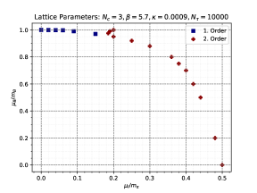
Figure 3: $\quantity(\mu_{I},\mu_{B})$-Phase diagram for $T\rightarrow 0$.

6 Conclusions

In this work, we have studied three-dimensional effective lattice theories for heavy quark QCD via a mean field approximation. This approach is promising because the effective theories represent $SU(3)$ spin models, and one expects at least qualitatively correct results for the phase structure of the effective theories. Indeed, for the simplest case representing the finite temperature pure gauge theory, a first-order deconfinement transition is observed, and the critical effective coupling is reproduced within $\sim$20% of the true answer.

We have then studied the situation close to the zero temperature limit, when both a baryon chemical potential and an isospin chemical potential are switched on. We obtain a clear picture with a first-order baryon onset transition for $\mu_{B}\approx m_{B},\mu_{I}=0$ and a second-order transition to a phase with isospin or Bose-Einstein condensate at $\mu_{I}\approx m_{\pi}/2,\mu_{B}=0$. These transitions are continuously connected and separate vacuum from matter. They meet in a branch point, where an additional second-order line emerges to separate the baryon region from the pion condensate region.

References

- [1] B.B. Brandt, G. Endrodi and S. Schmalzbauer, QCD phase diagram for nonzero isospin-asymmetry, Phys. Rev. D 97 (2018) 054514 [1712.08190].
- [2] P. de Forcrand, Simulating QCD at finite density, PoS LAT2009 (2009) 010 [1005.0539].
- [3] G. Aarts, Complex Langevin dynamics and other approaches at finite chemical potential, PoS LATTICE2012 (2012) 017 [1302.3028].
- [4] J.N. Guenther, Overview of the QCD phase diagram: Recent progress from the lattice, Eur. Phys. J. A 57 (2021) 136 [2010.15503].
- [5] M. Fromm, J. Langelage, S. Lottini and O. Philipsen, The QCD deconfinement transition for heavy quarks and all baryon chemical potentials, JHEP 01 (2012) 042 [1111.4953].
- [6] J. Langelage, S. Lottini and O. Philipsen, Centre symmetric 3d effective actions for thermal SU(N) Yang-Mills from strong coupling series, JHEP 02 (2011) 057 [1010.0951].
- [7] I. Montvay and G. Munster, Quantum fields on a lattice, Cambridge Monographs on Mathematical Physics, Cambridge University Press (3, 1997), 10.1017/CBO9780511470783.
- [8] J. Langelage, M. Neuman and O. Philipsen, Heavy dense QCD and nuclear matter from an effective lattice theory, JHEP 09 (2014) 131 [1403.4162].
- [9] J. Glesaaen, M. Neuman and O. Philipsen, Equation of state for cold and dense heavy QCD, JHEP 03 (2016) 100 [1512.05195].
- [10] J. Kim, A.Q. Pham, O. Philipsen and J. Scheunert, The SU(3) spin model with chemical potential by series expansion techniques, JHEP 10 (2020) 051 [2007.04187].
- [11] A.Q. Pham, J. Kim and O. Philipsen, Deconfinement critical point of heavy quark effective lattice theories, PoS LATTICE2021 (2022) 113 [2112.06505].
- [12] J.B. Kogut, M. Snow and M. Stone, Mean Field and Monte Carlo Studies of SU() Chiral Models in Three-dimensions, Nucl. Phys. B 200 (1982) 211.
- [13] F. Green and F. Karsch, Mean Field Analysis of SU(N) Deconfining Transitions in the Presence of Dynamical Quarks, Nucl. Phys. B 238 (1984) 297.
- [14] C. Gattringer, Flux representation of an effective Polyakov loop model for QCD thermodynamics, Nucl. Phys. B 850 (2011) 242 [1104.2503].
- [15] C. Konrad, O. Philipsen and J. Scheunert, Mean field approximation for effective theories of lattice QCD, in 39th International Symposium on Lattice Field Theory, 12, 2022 [2212.04417].
- [16] M. Fromm, J. Langelage, S. Lottini, M. Neuman and O. Philipsen, Onset Transition to Cold Nuclear Matter from Lattice QCD with Heavy Quarks, Phys. Rev. Lett. 110 (2013) 122001 [1207.3005].