Nucleon-nucleon scattering from distillation

Abstract

We report an ongoing analysis of nucleon-nucleon scattering based on finite-volume spectroscopy. The calculation is performed using the distillation method on eight lattice ensembles at the SU(3)-symmetric point with $m_{\pi}=m_{K}\approx 420$ MeV generated by CLS, covering a range of lattice spacings and volumes and previously used to study the $H$ dibaryon. We obtain nonzero signals for $S$, $P$, $D$, and $F$ waves as well as the mixing between spin-1 $S$ and $D$ waves. For $S$ waves, lattice artifacts are significant and tend to strengthen baryon-baryon interactions. In the deuteron and dineutron $S$ waves, we find virtual bound states.

1 Introduction

In Ref. [1], we reported a study of the $H$ dibaryon at the SU(3)-symmetric point where the $u$, $d$, and $s$ quark masses are set to their physical average value. Working at a fixed quark mass point, we were able to study a wide range of lattice spacings and multiple volumes. Surprisingly, we found that the binding energy of the $H$ dibaryon is significantly affected by discretization effects, ranging from about 5 MeV in the continuum to above 30 MeV on the coarsest lattice spacing.

In these proceedings, we report work in progress to study nucleon-nucleon scattering using the same dataset — at this stage, all results should be considered preliminary. Concerning the presence of $NN$ bound states at heavier-than-physical pion masses, there is a disagreement in the literature [2]: studies based on asymmetric point-source correlation functions (with a hexaquark interpolator at the source and a baryon-baryon interpolator at the sink) find a bound deuteron and dineutron [3, 4, 5, 6, 7, 8, 9], whereas studies using the variational method with a symmetric correlator matrix or using HAL QCD’s potential method find no bound state [10, 11, 12]. We also note the recent variational calculation from NPLQCD [13, 14] using ensembles previously employed in Refs. [3, 5, 9] that appears to be consistent with [11] but did not make a final decision about the presence of a bound state.

In the next section, we briefly summarize our methodology; in Section 3, we show the finite-volume and nonzero-lattice-spacing spectra; in Section 4, we study the $S$-wave phase shifts while neglecting higher partial waves; in Section 5, we show some higher partial waves; and in Section 6, we analyze the mixing between $S$ and $D$ waves. Finally, we give our conclusions.

2 Lattice setup

The details of our calculation are the same as in Ref. [1]. Matrices of two-point correlation functions were computed using the distillation method [15] on eight ensembles with nonperturbatively $O(a)$-improved Wilson-clover fermions generated by CLS [16] with $m_{\pi}=m_{K}\approx 420$ MeV, spanning six lattice spacings from 0.039 to 0.099 fm and $m_{\pi}L$ varying between 4.4 and 6.4.

Our analysis of the spectra is based on finite-volume quantization conditions [17, 18, 19, 20]. Roughly following Ref. [21], the finite-volume spectrum is given by solutions of

$$\det\left[\tilde{K}^{-1}(p^{2})-B(p^{2})\right]=0,$$ (1)

where $\tilde{K}$ contains the scattering amplitude and $B$ depends on the volume, $\vec{P}$, and irreducible representation of the little group of $\vec{P}$. In this work, our preferred kinematic variable is the centre-of-mass momentum $p^{2}\equiv(E_{\text{cm}}/2)^{2}-m^{2}$. Given an ansatz for $\tilde{K}^{-1}(p^{2})$, we find the solutions $\{p^{2}\}$ and compare them with the observed spectrum, performing a correlated least-squares minimization.

Here we study the flavour septenvigintuplet, which lies in the symmetric product of two octets and contains $NN$ $I=1$, and the antidecuplet, which lies in the antisymmetric product and contains $NN$ $I=0$. Our interpolating operators are formed from linear combinations of products of momentum-projected single-baryon interpolators and have definite flavour, total momentum $\vec{P}$, irrep, and two-baryon spin. Although spin is not a preserved quantum number, both the scattering amplitude for identical baryons and the two-particle finite-volume quantization condition are diagonal in spin, implying that spin zero and spin one can be analyzed separately. Furthermore, we observe that every state overlaps largely with operators with only one spin, allowing us to sort the states into spin zero or one.

3 Nucleon-nucleon spectra

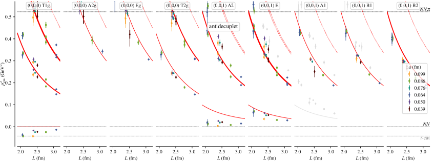
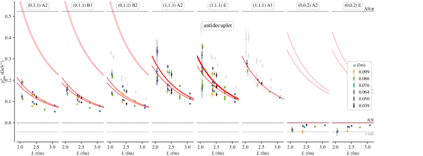
Figure 1: Antidecuplet ($NN$ $I=0$) spin-one spectrum for various total momenta and irreps: $p^{2}$ versus $L$. Red curves show noninteracting levels with a thickness proportional to the degeneracy; dashed curves show the lowest levels for which an interpolating operator was not included. Points correspond to lattice energy levels, with the thin outer error bar including an estimate of systematic uncertainty based on varying the plateau fit range. Gray points indicate levels that are identified as spin zero. Horizontal lines give the locations of thresholds and the $t$-channel cut.

We perform fits to ratios between diagonalized two-baryon correlators and the product of two single-baryon correlators to obtain energy differences from noninteracting levels. The systematic uncertainty is estimated using an alternative fit range. When we fit to the spectra to determine scattering amplitudes, currently we follow the same approach as Ref. [1] and treat this systematic as fully correlated, which means that it tends not to significantly reduce $\chi^{2}$; in the future, we may decide to change this. Also following Ref. [1], we use bootstrap to estimate statistical errors of the scattering parameters and fit the alternative spectra to estimate part of the systematic uncertainty.

A large number of energy levels is obtained. For example, the isospin-zero spin-one case is shown in Fig. 1, where we obtain over 300 levels. Fitting these will be a challenge and will require at minimum the ${}^{3}S_{1}$, ${}^{3}D_{1}$, ${}^{3}D_{2}$, and ${}^{3}D_{3}$ phase shifts together with the mixing angle for $J=1$, all of which depend on $p^{2}$ and may also be affected by lattice artifacts.

For many energy levels, a pattern is visible across the different ensembles similar to what was observed for the $H$ dibaryon: coarser ensembles produce lower-lying energies, generally corresponding to a stronger attraction. The long-sought-after splitting between the ground states in the A2 and E irreps in frame $(0,0,1)$ is also evident: this is a clear signal of mixing between ${}^{3}S_{1}$ and ${}^{3}D_{1}$ [22].

4 $S$-wave phase shifts

We begin by neglecting $D$-wave contributions and choosing energy levels to minimize the influence of higher partial waves. Under this approximation, each energy level directly yields the $S$-wave phase shift at that energy.

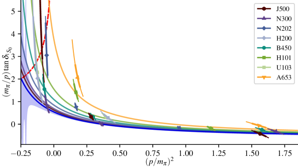
Figure 2: Septenvigintuplet ($NN$ $I=1$) ${}^{1}S_{0}$ phase shift: $p^{-1}\tan\delta$ versus $p^{2}$, normalized with the pion mass. Darker and more purple points and curves correspond to finer lattice spacings and pale points indicate the two small-volume ensembles. The blue curve with error band is the continuum limit of the fit. Intersections with the red dashed curve correspond to virtual state poles.

For the 27-plet ($NN$ $I=1$), we observe that the phase shift passes through zero above threshold while becoming large below threshold. This leads us to use a rational function as the fit ansatz, $p\cot\delta(p)=(c_{0}+c_{1}p^{2})/(1+c_{2}p^{2})$, where $c_{i}$ are affine functions of $a^{2}$. We select the ground and first-excited state in the rest frame irrep A1g, along with the ground state in the first moving frame irrep A1. On the two small-volume ensembles, we exclude the rest-frame excited state, since it lies above the $N\Delta$ threshold. The fit produces a rough description of the data, but quantitatively it is not particularly good, with $\chi^{2}/\text{dof}=23/16$. The data and the fit are shown in Fig. 2. The phase shift tends to decrease as the continuum limit is approached. There is a virtual state pole, which moves further below threshold in the continuum.

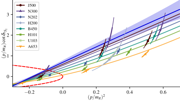
Figure 3: Antidecuplet ($NN$ $I=0$) ${}^{3}S_{1}$ phase shift, in the approximation that the ${}^{3}D_{1}$ partial wave and mixing with it vanish. See the caption of Fig. 2. An intersection the red dashed curve corresponds to a pole in the scattering amplitude: a virtual state if on the upper branch and a bound state if on the lower branch.

For the antidecuplet ($NN$ $I=0$), the presence of mixing between ${}^{3}S_{1}$ and ${}^{3}D_{1}$ partial waves complicates the analysis. For a first attempt, in the first and second moving frames we take the helicity-averaged ground-state levels [22]. In frame $(0,0,1)$, this corresponds to averaging the energy levels in irreps E and A2 with weights 2 and 1 to account for the fact that two of three helicities lie in the E irrep. We then treat the resulting averaged levels as arising from a purely $S$-wave interaction. We use a quadratic polynomial in $p^{2}$ with coefficients that are affine functions of $a^{2}$ as our fit ansatz for $p\cot\delta(p)$, which again yields worse-than-desired fit quality but still roughly describes the data: $\chi^{2}/\text{dof}=32/14$. This is shown in Fig. 3; as in previous cases, we find that going to finer lattice spacings produces a weaker interaction. For our coarsest lattice spacing, there is perhaps a bound state at threshold, but this turns into a virtual state and moves below threshold in the continuum. Note, however, that the usefulness of the helicity-averaged approximation is demonstrated empirically in Ref. [22] based on experimentally measured scattering amplitudes, and its validity should likewise be checked for the setup used here. We also note that our lowest-lying levels are very close to the $t$-channel cut, where existing quantization conditions are not valid; an approach that accounts for the leading $t$-channel exchange was presented at this conference [23].

5 Higher partial waves

Our data are also sensitive to higher partial waves. The simpler cases are those that do not mix, i.e. those with orbital and total angular momentum equal ($\ell=J$) as well as ${}^{3}P_{0}$. For the corresponding $P$ and $D$ waves, there always exists at least one frame and irrep for which no other equal or lower partial wave contributes. Thus, neglecting higher partial waves, each energy level in these irreps yields the corresponding phase shift at that energy level.

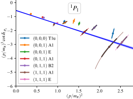
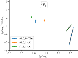
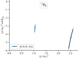
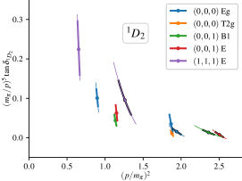
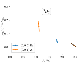
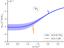
Figure 4: Higher partial waves from ensembles N202 ($L/a=48$, solid) and H200 ($L/a=32$, with black outline) with $a=0.064$ fm. First row: $P$ waves, $p^{3}\cot\delta$ versus $p^{2}$. Second row: $D$ and $F$ waves, $p^{-(2\ell+1)}\tan\delta$ versus $p^{2}$. The ${}^{1}P_{1}$, ${}^{3}D_{2}$, and ${}^{1}F_{3}$ partial waves have $I=0$, while ${}^{1}D_{2}$, ${}^{3}P_{1}$, and ${}^{3}P_{0}$ have $I=1$. For ${}^{1}P_{1}$, we have omitted the lowest-lying level in $(1,1,1)$ A1, which is more strongly influenced by the ${}^{1}F_{3}$ phase shift. The blue curves show the fit to all ensembles depicted in Fig. 5.

Figure 4 shows the data for two ensembles at a single lattice spacing. For the spin-zero cases, many energy levels are obtained, which yields a clear picture of the phase shift. In the spin one cases, the increased number of partial waves reduces the number of levels useful in this way, but we still obtain a good number of constraints on the phase shifts.

For a full analysis of the spectrum, levels that provide information about more than one partial wave can also be included, which will yield additional constraints on the phase shifts. An example fit for ${}^{1}P_{1}$ and ${}^{1}F_{3}$ is shown in Figs. 4 and 5: we use the four-parameter ansatz

$$p^{3}\cot\delta_{{}^{1}P_{1}}=c_{0}+c_{1}p^{2},\qquad p^{7}\cot\delta_{{}^{1}F_{3}}=c_{2}+c_{3}p^{8},$$ (2)

which is designed to make $\delta_{{}^{1}F_{3}}$ go to zero at large $p^{2}$. Assuming no discretization effects, we obtain a good fit to all ensembles with $\chi^{2}/\text{dof}=51/72$. This suggests that lattice artifacts may be less relevant for higher partial waves. Here it was essential to include the $F$ wave; neglecting this is partly responsible for the disagreement between the curve and the points for ${}^{1}P_{1}$ in Fig. 4.

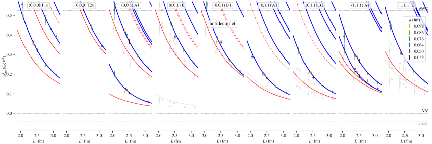
Figure 5: Antidecuplet ($NN$ $I=0$) spin-zero spectrum. See the caption of Fig. 1. The blue curves show the fit described in the text.

6 ${}^{3}S_{1}$–${}^{3}D_{1}$ partial wave mixing

For the coupled ${}^{3}S_{1}$ and ${}^{3}D_{1}$ partial waves, we use the Blatt-Biedenharn parametrization [24],

$$\tilde{K}^{-1}=\begin{pmatrix}1&0\\ 0&p^{2}\end{pmatrix}\begin{pmatrix}\cos\epsilon_{1}&-\sin\epsilon_{1}\\ \sin\epsilon_{1}&\cos\epsilon_{1}\end{pmatrix}\begin{pmatrix}p\cot\delta_{1\alpha}&0\\ 0&p\cot\delta_{1\beta}\end{pmatrix}\begin{pmatrix}\cos\epsilon_{1}&\sin\epsilon_{1}\\ -\sin\epsilon_{1}&\cos\epsilon_{1}\end{pmatrix}\begin{pmatrix}1&0\\ 0&p^{2}\end{pmatrix},$$ (3)

which encodes the diagonalization of the S-matrix. In the limit of zero mixing angle $\epsilon_{1}$, the $\alpha$ wave corresponds to ${}^{3}S_{1}$ and the $\beta$ wave to ${}^{3}D_{1}$. Using the approximation $\delta_{1\beta}=0$, each energy level imposes a constraint on the $(p^{-2}\tan\epsilon_{1},p\cot\delta_{1\alpha})$ plane:

$$p\cot\delta_{1\alpha}=\frac{B_{00}+(B_{01}+B_{10})x+B_{11}x^{2}}{1+p^{4}x^{2}},\quad x=p^{-2}\tan\epsilon_{1},$$ (4)

where $B_{ij}$ is the finite-volume matrix $B(p^{2})$.

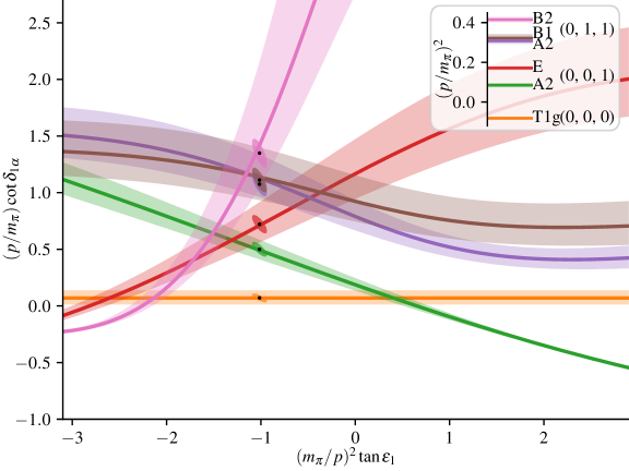
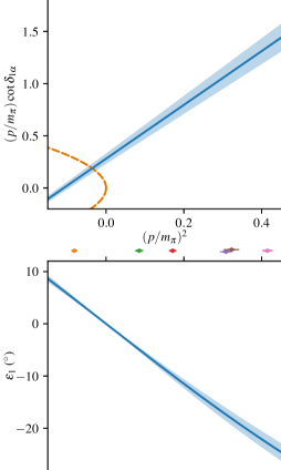
Figure 6: Ensemble N202: $\alpha$-wave phase shift and $J=1$ mixing angle, assuming $D$-wave phase shifts vanish. Left: constraints imposed by the different energy levels, with inset indicating the $p^{2}$ values. The points with error ellipses show the fit, evaluated at the corresponding $p^{2}$. Right: fitted $p\cot\delta_{1\alpha}$ and $\epsilon_{1}$ versus $p^{2}$.

For ensemble N202 (our largest volume), these constraints are shown for ground states in the rest frame and first two moving frames in Fig. 6. In the moving frames, different irreps provide quite different constraints and there is sensitivity to the mixing angle. We fit these six energy levels with the simple three-parameter ansatz

$$p\cot\delta_{1\alpha}=c_{1}+c_{2}p^{2},\qquad p^{-2}\tan\epsilon_{1}=c_{3},$$ (5)

obtaining $\chi^{2}/\text{dof}=1.2/3$, and the fit results are also shown in the figure. Like for the analysis using the helicity-averaged approximation, we find a virtual state pole. Above threshold, the mixing angle is negative, which should be contrasted with the positive mixing angle observed in experiments [22].

7 Conclusions

Using the distillation method, we were able to employ many interpolating operators and obtain a large number of finite-volume nucleon-nucleon energy levels. Similar to what was found in our study of the $H$ dibaryon, discretization effects appear to be significant also for the $NN$ spectrum. With the action used by CLS, lattice artifacts tend to strengthen $S$-wave baryon-baryon interactions. It appears that large lattice artifacts will add to the numerous existing challenges for computing the physical deuteron’s small binding energy.

We find virtual state poles in the $I=0$ and $I=1$ $NN$ $S$ waves at the SU(3)-symmetric point. Together with the opposite sign for the mixing angle $\epsilon_{1}$, this suggests that lighter pion masses will be needed to connect with the physics of the deuteron.

References

- [1] J.R. Green, A.D. Hanlon, P.M. Junnarkar and H. Wittig, Weakly bound dibaryon from SU(3)-flavor-symmetric QCD, Phys. Rev. Lett. 127 (2021) 242003 [2103.01054].
- [2] HAL QCD collaboration, Are two nucleons bound in lattice QCD for heavy quark masses? Consistency check with Lüscher’s finite volume formula, Phys. Rev. D 96 (2017) 034521 [1703.07210].
- [3] NPLQCD collaboration, Light nuclei and hypernuclei from quantum chromodynamics in the limit of SU(3) flavor symmetry, Phys. Rev. D 87 (2013) 034506 [1206.5219].
- [4] K. Orginos, A. Parreño, M.J. Savage, S.R. Beane, E. Chang and W. Detmold, Two nucleon systems at from lattice QCD, Phys. Rev. D 92 (2015) 114512 [1508.07583].
- [5] NPLQCD collaboration, Baryon-baryon interactions and spin-flavor symmetry from lattice quantum chromodynamics, Phys. Rev. D 96 (2017) 114510 [1706.06550].
- [6] NPLQCD collaboration, Low-energy scattering and effective interactions of two baryons at MeV from lattice quantum chromodynamics, Phys. Rev. D 103 (2021) 054508 [2009.12357].
- [7] T. Yamazaki, K.-i. Ishikawa, Y. Kuramashi and A. Ukawa, Helium nuclei, deuteron and dineutron in 2+1 flavor lattice QCD, Phys. Rev. D 86 (2012) 074514 [1207.4277].
- [8] T. Yamazaki, K.-i. Ishikawa, Y. Kuramashi and A. Ukawa, Study of quark mass dependence of binding energy for light nuclei in flavor lattice QCD, Phys. Rev. D 92 (2015) 014501 [1502.04182].
- [9] E. Berkowitz, T. Kurth, A. Nicholson, B. Joó, E. Rinaldi, M. Strother et al., Two-nucleon higher partial-wave scattering from lattice QCD, Phys. Lett. B 765 (2017) 285 [1508.00886].
- [10] HAL QCD collaboration, Two-baryon potentials and -dibaryon from 3-flavor lattice QCD simulations, Nucl. Phys. A 881 (2012) 28 [1112.5926].
- [11] B. Hörz et al., Two-nucleon -wave interactions at the SU(3) flavor-symmetric point with : A first lattice QCD calculation with the stochastic Laplacian Heaviside method, Phys. Rev. C 103 (2021) 014003 [2009.11825].
- [12] A. Nicholson et al., Resolving the controversy: a direct comparison of methods, PoS LATTICE2022 071.
- [13] S. Amarasinghe, R. Baghdadi, Z. Davoudi, W. Detmold, M. Illa, A. Parreño et al., A variational study of two-nucleon systems with lattice QCD, 2108.10835.
- [14] M. Wagman et al., Two-baryon variational spectroscopy, PoS LATTICE2022 088.
- [15] Hadron Spectrum collaboration, Novel quark-field creation operator construction for hadronic physics in lattice QCD, Phys. Rev. D 80 (2009) 054506 [0905.2160].
- [16] M. Bruno et al., Simulation of QCD with N 2 1 flavors of non-perturbatively improved Wilson fermions, JHEP 02 (2015) 043 [1411.3982].
- [17] M. Lüscher, Two-particle states on a torus and their relation to the scattering matrix, Nucl. Phys. B 354 (1991) 531.
- [18] K. Rummukainen and S.A. Gottlieb, Resonance scattering phase shifts on a non-rest-frame lattice, Nucl. Phys. B 450 (1995) 397 [hep-lat/9503028].
- [19] R.A. Briceño, Z. Davoudi and T.C. Luu, Two-nucleon systems in a finite volume: Quantization conditions, Phys. Rev. D 88 (2013) 034502 [1305.4903].
- [20] R.A. Briceño, Two-particle multichannel systems in a finite volume with arbitrary spin, Phys. Rev. D 89 (2014) 074507 [1401.3312].
- [21] C. Morningstar, J. Bulava, B. Singha, R. Brett, J. Fallica, A. Hanlon et al., Estimating the two-particle -matrix for multiple partial waves and decay channels from finite-volume energies, Nucl. Phys. B 924 (2017) 477 [1707.05817].
- [22] R.A. Briceño, Z. Davoudi, T. Luu and M.J. Savage, Two-nucleon systems in a finite volume. II. coupled channels and the deuteron, Phys. Rev. D 88 (2013) 114507 [1309.3556].
- [23] A.B. Raposo et al., Finite-volume formalism on the -channel cut, PoS LATTICE2022 051.
- [24] J.M. Blatt and L.C. Biedenharn, Neutron-proton scattering with spin-orbit coupling. I. General expressions, Phys. Rev. 86 (1952) 399.
- [25] Jülich Supercomputing Centre, JUQUEEN: IBM Blue Gene/Q supercomputer system at the Jülich Supercomputing Centre, J. Large-Scale Res. Facil. 1 (2015) A1.
- [26] Jülich Supercomputing Centre, JURECA: Modular supercomputer at Jülich Supercomputing Centre, J. Large-Scale Res. Facil. 4 (2018) A132.
- [27] Jülich Supercomputing Centre, JUWELS: Modular tier-0/1 supercomputer at the Jülich Supercomputing Centre, J. Large-Scale Res. Facil. 5 (2019) A135.
- [28] SciDAC, LHPC, UKQCD collaboration, The Chroma software system for lattice QCD, Nucl. Phys. B (Proc. Suppl.) 140 (2005) 832 [hep-lat/0409003].
- [29] A. Stathopoulos and J.R. McCombs, PRIMME: PReconditioned Iterative MultiMethod Eigensolver—methods and software description, ACM Trans. Math. Softw. 37 (2010) 21:1.
- [30] M. Lüscher and S. Schaefer, “openQCD.” http://luscher.web.cern.ch/luscher/openQCD/, 2012.
- [31] D.G.A. Smith and J. Gray, opt_einsum - A Python package for optimizing contraction order for einsum-like expressions, J. Open Source Softw. 3(26) (2018) 753.
- [32] C. Morningstar, “SigMonD.” https://github.com/andrewhanlon/sigmond, Feb., 2021.
- [33] C.R. Harris, K.J. Millman, S.J. van der Walt, R. Gommers, P. Virtanen, D. Cournapeau et al., Array programming with NumPy, Nature 585 (2020) 357 [2006.10256].
- [34] P. Virtanen, R. Gommers, T.E. Oliphant, M. Haberland, T. Reddy, D. Cournapeau et al., SciPy 1.0: fundamental algorithms for scientific computing in Python, Nature Methods 17 (2020) 261 [1907.10121].
- [35] J.D. Hunter, Matplotlib: A 2D graphics environment, Comput. Sci. Eng. 9 (2007) 90.