Independent Components of Word Embeddings
Represent Semantic Features

Abstract

Independent Component Analysis (ICA) is an algorithm originally developed for finding separate sources in a mixed signal, such as a recording of multiple people in the same room speaking at the same time. It has also been used to find linguistic features in distributional representations. In this paper, we used ICA to analyze words embeddings. We have found that ICA can be used to find semantic features of the words and these features can easily be combined to search for words that satisfy the combination. We show that only some of the independent components represent such features, but those that do are stable with regard to random initialization of the algorithm.

Independent Components of Word Embeddings
Represent Semantic Features

Tomáš Musil Charles University musil@ufal.mff.cuni.cz                        David Mareček Charles University marecek@ufal.mff.cuni.cz

1 Introduction

In this paper, we focus on examining word embeddings using Independent Component Analysis (ICA). Unlike PCA, it allows to represent a word with an unstructured set of features, without some of them being necessarily more important than others. ICA Comon (1994) is an algorithm originally developed for finding separate sources in a mixed signal, such as a recording of multiple people in the same room speaking at the same time. In the past, it was used for automatic extraction of features of words Honkela et al. (2010). We are interested in what we may learn with this technique about more recent word representations.

2 Independent Component Analysis

The ICA algorithm Hyvärinen and Oja (2000) consists of:

1. optional dimension reduction, usually with Principal Component Analysis (PCA),

2. centering the data and whitening them (setting variance of each component to 1),

3. iteratively finding directions in the data that are the most non-Gaussian.

The last step is based on the assumption of the central limit theorem: the mixed signal is a sum of independent variables, therefore it should be closer to the normal distribution than the variables themselves.

We are using the scikit-learn Pedregosa et al. (2011) implementation of the FastICA algorithm Hyvärinen (1999).

The algorithm is stochastic, every run gives a slightly different result.

We have tested the consistecy of individual runs by correlating two different runs of ICA on the same word embeddings. In Figure 1, which shows a correlation matrix for two instances of ICA, we see that one component from one run mostly corresponds to one component from the other run.

ICA may be an interesting tool for analysis of word embeddings also from a theoretical point of view. Following Musil (2021), we believe that it might be useful to conceptualize meaning of an expression as a combination of various components. These components would emerge from the use of the expression in context. Each of them would represent a specific relation to other expressions. The components would be continuous and will not form a simple tree hierarchy. ICA of word embeddings is a plausible candidate for such conceptualization, because unlike PCA, it allows to represent a word with an unstructured set of features, without some of them being necessarily more important than others.

Honkela et al. (2010) argue that ICA of word representations is also plausible from the perspective of cognitive linguistics, because it facilitates the emergence of sparsely encoded features by analysing the use of words in their context.

3 Data and Component Annotation

The English corpus that we used is the One Billion Word Benchmark (Chelba et al., 2013).

We have trained word2vec Mikolov et al. (2013) embeddings on the corpus with 512 dimensions and run ICA on them.

The distribution of words along a component usually follows a pattern: most words are located around 0 and a smaller group of words is separated in either the positive or the negative direction (due to the nature of the ICA algorithm, the polarity of each component is arbitrary). In Figure 2, this pattern of one-sidedness of the components is illustrated by plotting the distribution along a component, of the words for which that particular component is the highest one (in absolute value), against the rest of the words. We see two distinct characteristic patterns of this distribution: either most of these words is located in one of the positive/negative half-spaces, or there is relatively low number of these words and they are spread evenly on both sides.

We hired one annotator whose task was to manually annotate the meaning of individual components. For each component and both negative and positive directions, the annotator had a list of top 50 words in that component (and direction) and also a list of words for which the component in that direction is the largest (in absolute value) of the components. The independent components were annotated with categories pertaining to these lists. For most of the components (378 out of 512) only one end of the component had a meaningful interpretation. For some components, the annotator did not find any meaningful interpretation for either of the ends (this was the case for 119 out of 512 components). In rare cases (15 out of 512) both ends of the component were annotated as meaningful. The annotator also classified the categories in metacategories (such as “sports”, “countries”, etc.). Out of the 378 identified components, 35 are related to sports, 28 to numbers, 26 to countries (and further 13 to particular states of the USA), etc. This corresponds to the distribution of topics in the training corpus, which consists mostly of news articles.

To experiment on texts from a different domain, we have also used the English side of the section c-fiction of the CzEng 1.7 corpus Bojar et al. (2016), containing 78M tokens (997k unique tokens) of short passages from various fiction books.

4 Results

Figure 1: Correlations of two different runs of ICA on the same data. It shows that ICA is fairly constistent, although due to the random initialization, the runs are not exactly the same. The rows of the matrix are sorted by the index of their maximum, so that we can easily see that one row approximately correlates to one column. Only the absolute value of the correlation coefficient matters, because the sign of each component is arbitrary and depends on random initialization.

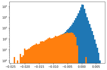
(a)

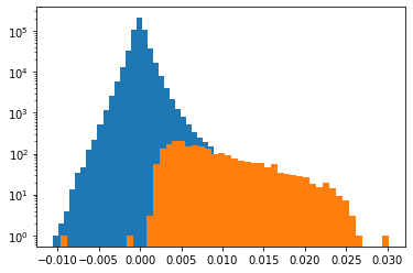
(b)

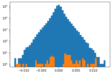
(c)

Figure 2: Histograms of distributions of words along a particular component. Orange bars represent words, for which the particular component is the largest (in absolute value) of their components. Blue bars represent the rest of the vocabulary. Note that the vertical axis is logarhitmic, otherwise the orange bars would be too low to be distinguishable. There are three typical shapes of these histograms: (a) orange mass in the negative direction, (b) orange mass in the positive direction, and (c) small amount of orange scattered randomly. This shows that the components usually capture some feature in one direction (a, b), which is arbitrary (property of the ICA algorithm), or contain random noise (c).

Figure 3: Histogram of ICA components and their correlations between different runs of the analysis. The green components were evaluated as containing semantic information, orange components as unsure, red components as not containing semantic information. The horizontal axis describes the maximal correlation coefficient for a given component. This shows that the components that were evaluated as representing sematic features are stable across multiple runs of the ICA algorithm.

Figure 4: Histogram of ICA components. For each component, words for which the particular component is the largest (in absolute value) are counted. We divide these words into two sets, based on whether this particular component has negative or positive value for the word. Then we compute how much of these words is contained in the larger of the two sets. This is what is represented on the horizontal axis. The value of 50% means that there is equal number of positive and negative values for the particular component among the words for which this is the largest component. The value of 100% means that all the words for which the component is the largest are on one side (either positive, or negative). This shows that the one-sided components were more likely to be labeled as representing a semantic feature, while components with less than 70% of words on one side were mostly unlabeled, implicitly considered to be random noise.

	tennis	football	Formula 1	basketball
Australia	Stosur, Lleyton, Dokic, Laver	Ashley-Cooper, Mortlock, Giteau, Viduka	Trulli, Jarno, MELBOURNE, Melbourne	Macklin, Bogut, Rossiter, JaJuan
Brazil	Thomaz, Paes, Bellucci, Amelie	Alves, Carvalho, Welbeck, Denilson	Interlagos, Barrichello, Massa, Brazilian	Barbosa, Machado, Leandro, Menezes
Canada	Dancevic, Aleksandra, Wozniak, Zimonjic	Bassong, Upson, Ameobi, Harmison	Kubica, Raikkonen, Heidfeld, Kimi	Bargnani, Calderon, Augustin, Delfino
China	Jie, Shuai, Zheng, Peng	Shui-bian, Akmal, Henan, Welbeck	melamine, Vettel, Lap, Xian	Jianlian, Deng, Ming, Yao
France	Paul-Henri, Benneteau, Jo-Wilfried, Monfils	Benzema, Abidal, Anelka, Chamakh	Todt, Prost, Renault, Bourdais	Batum, Mickael, Sacre, Dominique
Germany	Kohlschreiber, Schuettler, Zverev, Petzschner	Schweinsteiger, Ballack, Klose, Olic	Heidfeld, Timo, Rosberg, Vettel	Freshman, Winnenden, Kaman, Appel
Israel	Dudi, Sela, Shahar, Obziler	Benayoun, Yossi, Behrami, Ben-Haim	Dani, Button, Trulli, constructors	Omri, Casspi, Lazar, Beitenu
Japan	Sugiyama, Nishikori, Morita, Ayumi	Nakamura, Shunsuke, Nakajima, Mitsui	Nakajima, Kazuki, Fuji, Sato	Nakajima, Nikkei, Yasukuni, Sumitomo
Sweden	Arvidsson, Soderling, Nieminen, Bjorkman	Ibrahimovic, Olsson, Bendtner, Elmander	Spyker, Finnish, Vatanen, Kovalainen	Pedersen, Joakim, Landry, Scola

Table 1: Combinations of independent components. Rows are components representing states, columns are components representing sports. Each cell of the table shows 4 words for which the product of the corresponding components is the highest in the vocabulary. The words that we were able to determine to be correctly selected as the combination of the two components (e.g. “Ibrahimovic” really is a name of a swedish football player) are colored green.

The ICA algorithm always returns as many components as we specify before running it (up to the dimension of the original data). If the data was generated by a lower number of independent components and some random noise, ICA will return some components containing only the noise. We can see this effect in Figure 1. When we correlate components from two runs of ICA on the same data, we see that most of the components from the first run are strongly correlated one-to-one with components from the other run. Our hypothesis is that these are the independent components that represent independent features of words. The components that do not correlate are noise. Our annotation supports this hypothesis. In Figure 3 we see the histogram of ICA components from two different runs of the ICA algorithm. It shows that components that were annotated as interpretable are stable with different random initialization, while components that were annotated as components without interpretation generally do not have a strongly correlated counterpart when the model is run with different initialization.

Another hypothesis corroborated by the annotation is that the components that are one-sided (see Figure 2) are the ones that are interpretable, while the spread-out components contain only noise. As we can see in Figure 4, the more the component is one-sided, the more likely it is to be annotated as interpretable and vice versa. The side of the one-sided components that was annotated as interpretable was always the one with the higher ratio of words for which that particular component was the highest one.

The few components that were annotated differently from what we would expect can be explained by ascribing meaning to a random selection on the one side and failing to recognize patterns specific to the corpus on the other. There is, for example, a component representing words associated with blog post of a particular author, which is only apparent in retrospect after searching for some of the words in the training corpus, which was not available to the annotator.

vectors	intruder identified
word2vec	369 (36%)
ICA	475 (46%)

Table 2: Preliminary results (for a single annotator) of the word intruder test on the Billion corpus. For word2vec dimensions, the intruder word was identified less often than for the ICA dimensions.

We also used the word intruder test (Chang et al., 2009), that has been widely used in estimating interpretability (Subramanian et al., 2018). In this test, the annotators are presented with 5 words, 4 of which are the top 4 words for a particular component. The fifth word is an intruder, selected randomly from the top 10% of words from another randomly selected component. If the component is interpretable, the top words should form a coherent set and the annotators should be able to identify the intruder word.

Table 2 shows preliminary results of the intruder test. The ICA components seem to be more interpretable than the original word2vec embeddings. For the ICA components, we had the word intruder test annotated by three independent annotators. All three annotators agreed on the correct intruder word in 211 cases out of 1024 (512 components, 2 directions for each). For a random baseline, we would expect agreement on 8.1 cases ($1024\times(\frac{1}{5})^{3}$).

4.1 Combining the Components

As we have seen in Figure 2, each component is either positive, negative, or noisy. For each component, we can compute the mean value of that component for words for which this is the highest component in absolute value and then flip the sign of the component if the mean is negative. This does not affect the positive components. The negative components become positive and the noisy components are still noisy. In the rest of this section, we assume that this operation was carried out on the model and all of the components that represent semantic features do so in the positive direction.

We can combine a pair of components by searching for words for which the product of the components is the highest. For example, in our particular instance of ICA of Word2vec embeddings of the English side of the CzEng-fiction corpus, the 15 words for which the value of $C_{398}$ (component number 398) is the highest are the following: rumble, booming, roar, wail, sound, murmur, shouts, cries, louder, shrill, screams, noises, muffled, voices, howl We see that this components has high values for words associated with sound. For $C_{110}$, the top 15 words are associated with animals: cats, predators, rats, predator, lions, fox, rabbits, bears, wolves, lion, deer, dogs, mice, tigers, cat. If we search for the top 15 words for which $C_{398}\cdot C_{110}$ is the highest, we get the following:

sound $\ast$ animals: growl, barking, purr, growls, whine, baying, growling, howl, yelp, bleating, chirping, buzzing, squealing, squeals, crickets

Here are some further examples from the same model:

sound $\ast$ horses: hooves, hoofs, hoofbeats, snort, hoof, whinny, jingling, snorting, clop, clink, whinnying, thudding, jingle, shod, neighing

sound $\ast$ church: bells, chanting, prayers, hymns, hymn, chant, choir, preaching, bell, tolling, chants, chorus, peal, chime, tolled

sound $\ast$ play: melody, flute, music, musical, chords, orchestra, guitar, stringed, violin, trumpets, tune, accompaniment, piano, Bach, melodies

sound $\ast$ door: click, clang, creak, thud, clanged, clank, clink, splintering, clunk, squeak, groan, audible, snick, thunk, footsteps

clothing $\ast$ army: fatigues, uniforms, regimental, insignia, Infantry, uniform, tabs, breastplate, vests, stripes, Kevlar, Armored, helmets, outfit, pants

units $\ast$ money: dollars, cent, cents, francs, bucks, per, dollar, billion, roubles, shillings, million, percent, guineas, pounds, pence

In Table 4, we show results of combining components representing sports and countries in the Billion corpus. Notice that the name Nakajima occurs in three different columns and in fact refers to three different people (Nakajima Kazuki, Shoya, and Yoshifumi). This illustrates that the features are truly independent: being a name associated with one sport does not prevent the word to be associated with a different sport at the same time.

4.2 Contextual Embeddings

We have also examined embeddings from a pretrained BERT model Devlin et al. (2019). We followed Bommasani et al. (2020) and extracted static embeddings from the model by computing average vecors over all the occurences of a subword in the corpus.

We have found that the independent components of subwords often do not make much sense. There are component of subwords starting or ending with a particular letter. This seems to be a consequence of the WordPiece algorithm constructing the subwords from left to right in a greedy manner, resulting in breaking the words up in improper places.

We have also examined embeddings of words obtained by averaging the subword embeddings (as proposed by Bommasani et al. (2020)). In this case, most of the components are just grouping together words that contain a particular subword. The defining subword is often short and without any lexical meaning. In this case, the ICA method seems to highlight the artifacts of the tokenization, rather than features of language or the training corpus.

This may indicate, that although embeddings obtained through averaging contextual embeddings score higher than Word2vec in word similarity tasks, the space of Word2vec embeddings is in some sense better arranged to represent sematics. Further experiments are needed to corroborate this hypothesis and we believe this would be an intersting possibility for future work.

5 Related work

Väyrynen and Honkela (2005) devised a method to quantify how well the unsupervised features correspond to a set of supervised features. They compare SVD and ICA and conclude that ICA corresponds better to human intuition.

Musil (2019) examined the structure of word embeddings with PCA. They found that PCA dimensions correlate strongly with information about Part of Speech (POS) and that the shape of the space is strongly dependent on the task that the network is trained for.

Faruqui et al. (2015) and Subramanian et al. (2018) generated sparse interpretable representations from word embeddings. Unlike ICA, these are not simple projections of the original vectors.

Related work on examining vector representations in Natural Language Processing (NLP) was surveyed by Bakarov (2018). Further information can also be found in the overview of methods for analysing deep learning models for NLP by Belinkov and Glass (2019). For more on interpretation in general and unsupervised methods in examining word embeddings, see Mareček et al. (2020, Chapters 3 and 4).

6 Conclusion

ICA is capable of uncovering interesting patterns in the word embedding space. The independent components correspond to various features, that seem to be mostly semantic. These features tend to be binary and the components uni-directional: words on one end of the component have that feature, the rest of the words do not.

Some of the independent components seem to be random noise. We have demonstrated that the components for which we are able to find an iterpretation are stable with regards to random initialization of the ICA algorithm.

The independent components can be combined as semantic features by simple multiplication, giving high values to words that combine the semantic features associated with the multiplied components.

In case of representations derived from contextual embeddings, the independent components seem to pick up features related to tokenization rather than semantics, which leads to questions for future work in tokenization and interpretability.

References

- Bakarov (2018) Amir Bakarov. 2018. A Survey of Word Embeddings Evaluation Methods. arXiv:1801.09536 [cs]. ArXiv: 1801.09536.
- Belinkov and Glass (2019) Yonatan Belinkov and James Glass. 2019. Analysis Methods in Neural Language Processing: A Survey. Transactions of the Association for Computational Linguistics, 7:49–72.
- Bojar et al. (2016) Ondřej Bojar, Ondřej Dušek, Tom Kocmi, Jindřich Libovický, Michal Novák, Martin Popel, Roman Sudarikov, and Dušan Variš. 2016. CzEng 1.6: Enlarged Czech-English Parallel Corpus with Processing Tools Dockered. In Text, Speech, and Dialogue: 19th International Conference, TSD 2016, Lecture Notes in Artificial Intelligence, pages 231–238, Cham / Heidelberg / New York / Dordrecht / London. Springer International Publishing.
- Bommasani et al. (2020) Rishi Bommasani, Kelly Davis, and Claire Cardie. 2020. Interpreting Pretrained Contextualized Representations via Reductions to Static Embeddings. In Proceedings of the 58th Annual Meeting of the Association for Computational Linguistics, pages 4758–4781, Online. Association for Computational Linguistics.
- Chang et al. (2009) Jonathan Chang, Sean Gerrish, Chong Wang, Jordan Boyd-graber, and David Blei. 2009. Reading tea leaves: How humans interpret topic models. In Advances in Neural Information Processing Systems, volume 22. Curran Associates, Inc.
- Chelba et al. (2013) Ciprian Chelba, Tomas Mikolov, Mike Schuster, Qi Ge, Thorsten Brants, Phillipp Koehn, and Tony Robinson. 2013. One billion word benchmark for measuring progress in statistical language modeling. arXiv preprint arXiv:1312.3005.
- Comon (1994) Pierre Comon. 1994. Independent component analysis, a new concept? Signal processing, 36(3):287–314.
- Devlin et al. (2019) Jacob Devlin, Ming-Wei Chang, Kenton Lee, and Kristina Toutanova. 2019. Bert: Pre-training of deep bidirectional transformers for language understanding. ArXiv, abs/1810.04805.
- Faruqui et al. (2015) Manaal Faruqui, Yulia Tsvetkov, Dani Yogatama, Chris Dyer, and Noah A. Smith. 2015. Sparse overcomplete word vector representations. In Proceedings of the 53rd Annual Meeting of the Association for Computational Linguistics and the 7th International Joint Conference on Natural Language Processing (Volume 1: Long Papers), pages 1491–1500, Beijing, China. Association for Computational Linguistics.
- Honkela et al. (2010) Timo Honkela, Aapo Hyvärinen, and Jaakko J. Väyrynen. 2010. WordICA—emergence of linguistic representations for words by independent component analysis. Natural Language Engineering, 16(3):277–308.
- Hyvärinen and Oja (2000) A. Hyvärinen and E. Oja. 2000. Independent component analysis: algorithms and applications. Neural Networks, 13(4-5):411–430.
- Hyvärinen (1999) Aapo Hyvärinen. 1999. Fast and robust fixed-point algorithms for independent component analysis. IEEE transactions on Neural Networks, 10(3):626–634.
- Mareček et al. (2020) David Mareček, Jindřich Libovický, Tomáš Musil, Rudolf Rosa, and Tomasz Limisiewicz. 2020. Hidden in the Layers: Interpretation of Neural Networks for Natural Language Processing, volume 20 of Studies in Computational and Theoretical Linguistics. Institute of Formal and Applied Linguistics, Prague, Czechia. Backup Publisher: Institute of Formal and Applied Linguistics.
- Mikolov et al. (2013) Tomas Mikolov, Kai Chen, Gregory S. Corrado, and Jeffrey Dean. 2013. Efficient Estimation of Word Representations in Vector Space. CoRR, abs/1301.3781.
- Musil (2021) Tomáš Musil. 2021. Representations of meaning in neural networks for NLP: a thesis proposal. In Proceedings of the 2021 Conference of the North American Chapter of the Association for Computational Linguistics: Student Research Workshop, pages 24–31, Online. Association for Computational Linguistics.
- Musil (2019) Tomáš Musil. 2019. Examining Structure of Word Embeddings with PCA. In Text, Speech, and Dialogue, pages 211–223, Cham. Springer International Publishing.
- Pedregosa et al. (2011) F. Pedregosa, G. Varoquaux, A. Gramfort, V. Michel, B. Thirion, O. Grisel, M. Blondel, P. Prettenhofer, R. Weiss, V. Dubourg, J. Vanderplas, A. Passos, D. Cournapeau, M. Brucher, M. Perrot, and E. Duchesnay. 2011. Scikit-learn: Machine Learning in Python. Journal of Machine Learning Research, 12:2825–2830.
- Subramanian et al. (2018) Anant Subramanian, Danish Pruthi, Harsh Jhamtani, Taylor Berg-Kirkpatrick, and Eduard Hovy. 2018. Spine: Sparse interpretable neural embeddings. Proceedings of the AAAI Conference on Artificial Intelligence, 32(1).