Josephson transmission line revisited

Abstract

We consider the series-connected Josephson transmission line (JTL), constructed from Josephson junctions, capacitors and (possibly) resistors. We calculate the velocity of shocks in the discrete lossy JTL. We study thoroughly the continuum and the quasi-continuum approximations to the discrete JTL, both lossless and lossy. In the framework of these approximations we show that the compact travelling waves in the lossless JTL are the kinks and the solitons, and calculate their velocities. On top of each of the above mentioned approximations, we propose the simple wave approximation, which decouples the JTL equations into two separate equations for the right- and left-going waves. The approximation, in particular, allows to easily consider the formation of shocks in the lossy JTL.

I Introduction

The concept that in a nonlinear wave propagation system the various parts of the wave travel with different velocities, and that wave fronts (or tails) can sharpen into shock waves, is deeply imbedded in the classical theory of fluid dynamics whitham . The methods developed in that field can be profitably used to study signal propagation in nonlinear transmission lines french ; nouri ; neto ; nikoo ; silva ; wang ; rangel ; kyuregyan ; akem ; fairbanks . In the early studies of shock waves in transmission lines, the origin of the nonlinearity was due to nonlinear capacitance in the circuit landauer ; peng ; rabinovich .

Interesting and potentially important examples of nonlinear transmission lines are Josephson transmission lines (JTL) barone ; pedersen ; tinkham ; kadin , constructed from Josephson junctions (JJs), capacitors, and (possibly) resistors. The unique nonlinear properties of JTL allow to construct soliton propagators, microwave oscillators, mixers, detectors, parametric amplifiers, and analog amplifiers pedersen ; kadin ; tinkham .

Transmission lines formed by JJs connected in series were studied beginning from 1990s, though much less than transmission lines formed by JJs connected in parallel solitons . However, the former began to attract quite a lot of attention recently yaakobi ; brien ; macklin ; kochetov ; zorin ; basko ; dixon ; goldstein , especially in connection with possible JTL traveling wave parametric amplification white ; miano ; pekker .

The interest in studies of discrete nonlinear electrical transmission lines, in particular of lossy nonlinear transmission lines, has started some time ago rosenau ; chen ; mohebbi , but it became even more pronounced recently ricketts ; houwe ; katayama ; sekulic . These studies should be seen in the general context of waves in strongly nonlinear discrete systems kevrikidis0 ; english ; kevrikidis ; nesterenko0 ; malomed2 ; nesterenko ; malomed . A very informative and very recent review of nonlinear electric transmission networks one can find in Ref. malomed3 .

In our previous publications we considered travelling waves in the continuous kogan2 and the discrete kogan JTL. We have shown that such travelling waves are the kinks and the solitons in the lossless line and the shocks in the lossy line. In the present paper we rederive part of the results obtained previously in a more concise and physically appealing way and also generalize them. We must add that both previously and now our lossless JTL didn’t (doesn’t) contain the capacitor shunting the JJ, and our lossy JTL – did, which made (makes) the model of the JJ more realistic.

The rest of the paper is constructed as follows. In Section II we write down the Kirchhoff equations for the discrete JTL, both lossless and lossy, and calculate the velocity of shock, existing in the latter case. In Section III, on top of the continuum approximation, we formulate the simple wave approximation, which decouples two coupled continuum JTL equations into two separate equations for the right- and left-going waves. In Section IV we formulate the quasi-discrete approximation and show that the only compact travelling waves in the lossless JTL are the kinks and the solitons and calculate their velocities. In Section V we formulate the simple wave approximation to the quasi-continuum JTL equations. We conclude in Section VI. In the Appendix A we write down the Hamiltonian, describing the lossless JTL. In the Appendix B we present graphical analysis of the shocks. In the Appendix C we use Riemann method of characteristics to justify (up to a certain degree) the simple wave approximation.

II The discrete JTL

II.1 The lossless line

Consider the discrete model of lossless line, constructed from identical JJ and capacitors, which is shown on Fig. 1. We take as dynamical variables the phase differences (which we for brevity will call just phases) $\varphi_{n}$ across the JJs and the charges $q_{n}$ of the ground capacitors. (Note that the latter choice is different from what was done in our previous publications and in the Appendix A.)

Figure 1: Lossless discrete Josephson transmission line

The circuit equations are

$$\frac{\hbar}{2e}\frac{d\varphi_{n}}{dt} =\frac{1}{C}\left(q_{n-1}-q_{n}\right),$$ (1a)

$$\frac{dq_{n}}{dt} =I_{c}\left(\sin\varphi_{n}-\sin\varphi_{n+1}\right),$$ (1b)

where $C$ is the capacitance, and $I_{c}$ is the critical current of the JJ.

The compact waves we are considering are characterised by the boundary conditions

$$\lim_{n\to-\infty}\varphi=\varphi_{2}\;,\hskip 28.45274pt\lim_{n\to+\infty}\varphi=\varphi_{1},$$ (2)

$$\lim_{n\to-\infty}q=q_{2}\;,\hskip 28.45274pt\lim_{n\to+\infty}q=q_{1}\,.$$ (3)

(These conditions will remain the same after we include the losses.) Summing up (1) from the far left to the far right we obtain

$$\frac{\hbar}{2e}\sum_{n}\frac{d\varphi_{n}}{dt} =\frac{1}{C}\left(q_{2}-q_{1}\right),$$ (4a)

$$\sum_{n}\frac{dq_{n}}{dt} =I_{c}\left(\sin\varphi_{2}-\sin\varphi_{1}\right).$$ (4b)

The travelling wave solutions satisfy equations

$$\varphi_{n}(t) =\varphi(Ut-n\Lambda),$$ (5a)

$$q_{n}(t) =q(Ut-n\Lambda),$$ (5b)

where $\Lambda$ is the JTL period and $U$ is the travelling wave velocity. Hence keeping only the main harmonic in the Poisson summation formula for the sums in the l.h.s. of Eqs. (1), we can write down

$$\sum_{n}\frac{d\varphi_{n}}{dt} =\frac{U}{\Lambda}\left(\varphi_{2}-\varphi_{1}\right),$$ (6a)

$$\sum_{n}\frac{dq_{n}}{dt} =\frac{U}{\Lambda}\left(q_{2}-q_{1}\right),$$ (6b)

and (4) becomes

$$\frac{\hbar U}{2e\Lambda}\left(\varphi_{2}-\varphi_{1}\right) =\frac{1}{C}\left(q_{2}-q_{1}\right),$$ (7a)

$$\frac{U}{\Lambda}\left(q_{2}-q_{1}\right) =I_{c}\left(\sin\varphi_{2}-\sin\varphi_{1}\right),$$ (7b)

Excluding $q_{2}-q_{1}$ we obtain

$$\overline{U}^{2}\left(\varphi_{1}-\varphi_{2}\right)=\sin\varphi_{1}-\sin\varphi_{2};$$ (8)

for any velocity $V$ in this paper

$$\overline{V}\equiv\frac{\sqrt{L_{J}C}}{\Lambda}V.$$ (9)

where $L_{J}=\hbar/(2eI_{c})$. The velocity $U$ should be compared with is the velocity $u(\varphi)$ of propagation of small amplitude disturbances on a homogeneous background $\varphi$, which is given by the equation kogan2

$$\overline{u}(\varphi)=\sqrt{\cos\varphi}.$$ (10)

(Everywhere in this paper we consider only the case $-\pi/2<\varphi<\pi/2$.)

We must admit that, strictly speaking, ignoring of the higher harmonics in the Poisson summation formula which led to (6) can be justified only when the space scale of the solutions is much larger than $\Lambda$. In Ref. kogan it was shown that this is true for weak waves (the definition of the weak wave see below). However further on we’ll forget about this limitation.

Differentiating (1a) with respect to $t$ and substituting $dq_{n}/dt$ from Eq. (1b), we obtain closed equation for $\varphi_{n}$

$$\frac{d^{2}\varphi_{n}}{d\tau^{2}}=\sin\varphi_{n+1}-2\sin\varphi_{n}+\sin\varphi_{n-1},$$ (11)

where we introduced the dimensionless time $\tau=t/\sqrt{L_{J}C}$. Equation (11) will be used in Section IV.

II.2 The lossy line

Now let us consider the JTL with the capacitors and resistors shunting the JJs and (resistors) in series with the ground capacitors, shown on Fig. 2. As the result, Eq. (1) changes to

$$\frac{\hbar}{2e}\frac{d\varphi_{n}}{dt} =\left(\frac{1}{C}+R\frac{d}{dt}\right)\left(q_{n-1}-q_{n}\right),$$ (12a)

$$\frac{dq_{n}}{dt} =I_{c}\sin\varphi_{n}-I_{c}\sin\varphi_{n+1}$$

$$+\left(\frac{\hbar}{2eR_{J}}\frac{d}{dt}+C_{J}\frac{\hbar}{2e}\frac{d^{2}}{dt^{2}}\right)\left(\varphi_{n}-\varphi_{n+1}\right),$$ (12b)

where $R$ is the ohmic resistor in series with the ground capacitor, and $C_{J}$ and $R_{J}$ are the capacitor and the ohmic resistor shunting the JJ.

Figure 2: Discrete Josephson transmission line with the capacitor and the resistor shunting the JJ and another resistor in series with the ground capacitor

Summing up (12) from the far left to the shock to the far right, we obtain instead of (7)

$$\frac{\hbar U}{2e\Lambda}\left(\varphi_{1}-\varphi_{2}\right) =\left(\frac{1}{C}+R\frac{d}{dt}\right)\left(q_{2}-q_{1}\right),$$ (13a)

$$\frac{U}{\Lambda}\left(q_{1}-q_{2}\right) =I_{c}\left(\sin\varphi_{2}-\sin\varphi_{1}\right)$$

$$+\left(\frac{\hbar}{2eR_{J}}\frac{d}{dt}\right. +\left.C_{J}\frac{\hbar}{2e}\frac{d^{2}}{dt^{2}}\right)\left(\varphi_{2}-\varphi_{1}\right).$$ (13b)

All the time derivatives are equal to zero, and we recover equations (7), which are presented graphically in the Appendix B. From (7) follows (8), hence we obtain for the shock velocity equation kogan2 ; kogan

$$\overline{U}^{2}_{\text{sh}}(\varphi_{1},\varphi_{2})=\frac{\sin\varphi_{1}-\sin\varphi_{2}}{\varphi_{1}-\varphi_{2}}.$$ (14)

The situation is similar to that in fluid dynamics landau2 : the losses are necessary for the existence of the shock but don’t influence the shock velocity.

The resistance in series with the ground capacitor doesn’t have any clear cut physical realization, so from now on we’ll put $R=0$. A more realistic model would include resistance parallel to the capacitor, but we postpone such generalization until later time.

III The continuum approximation

III.1 The lossless line

Let us write down Eq. (1) in the continuum approximation, that is let us treat $n$ as the continuous variable $Z$ and approximate the finite differences in the r.h.s. of the equations as the first derivative with respect to $Z$. After which (1) takes the form

$$\frac{\partial\varphi}{\partial\tau} =-\frac{\partial Q}{\partial Z},$$ (15a)

$$\frac{\partial Q}{\partial\tau} =-\cos\varphi\frac{\partial\varphi}{\partial Z},$$ (15b)

where we introduced the dimensionless charge $Q=q/(I_{c}\sqrt{L_{J}C})$.

III.1.1 The simple wave approximation

The simple wave approximation is decoupling of the wave equation into two separate equations for the right- and left-going waves. To achieve that aim let us assume that $Q$ is a function of $\varphi$. Then we have

$$\frac{\partial Q}{\partial Z} =\frac{dQ}{d\varphi}\frac{\partial\varphi}{\partial Z},$$ (16a)

$$\frac{\partial Q}{\partial\tau} =\frac{dQ}{d\varphi}\frac{\partial\varphi}{\partial\tau}.$$ (16b)

Substituting (16) into (15) and excluding $dQ/d\varphi$ we obtain kogan2

$$\frac{\partial\varphi}{\partial\tau}=\pm\sqrt{\cos\varphi}\frac{\partial\varphi}{\partial Z}.$$ (17)

On the other hand, excluding the partial derivatives after the substitution we obtain

$$\left(\frac{dQ}{d\varphi}\right)^{2}=\cos\varphi\Rightarrow Q=\pm\int\sqrt{\cos\varphi}d\varphi.$$ (18)

Another line of reasoning which can lead from to (15) to (17) and (18) is based on Riemann method of characteristics landau2 and is presented in the Appendix C.

III.2 The lossy line

Applying the continuum approximation to (12) we obtain

$$\frac{\partial\varphi}{\partial\tau} =-\frac{\partial Q}{\partial Z},$$ (19a)

$$\frac{\partial Q}{\partial\tau} =-\frac{\partial\sin\varphi}{\partial Z}-\frac{Z_{J}}{R_{J}}\frac{\partial^{2}\varphi}{\partial\tau\partial Z}-\frac{C_{J}}{C}\frac{\partial^{3}\varphi}{\partial\tau^{2}\partial Z},$$ (19b)

where $Z_{J}\equiv\sqrt{L_{J}/C}$ is the characteristic impedance of the JTL. We can exclude $Q$ from (19) and obtain closed equation for $\varphi$

$$\frac{\partial^{2}\varphi}{\partial\tau^{2}}=\frac{\partial^{2}}{\partial Z^{2}}\left(\sin\varphi+\frac{Z_{J}}{R_{J}}\frac{\partial\varphi}{\partial\tau}+\frac{C_{J}}{C}\frac{\partial^{2}\varphi}{\partial\tau^{2}}\right).$$ (20)

If we expand the sine function in the r.h.s. of (20) in Taylor series, keep the first two terms of the expansion, substitute $\varphi=\partial\widetilde{\varphi}/\partial Z$ and integrate the resulting equation with respect to $Z$ we obtain

$$\frac{\partial^{2}\widetilde{\varphi}}{\partial\tau^{2}}=\frac{\partial^{2}\widetilde{\varphi}}{\partial Z^{2}}-\frac{1}{6}\frac{\partial}{\partial Z}\left(\frac{\partial\widetilde{\varphi}}{\partial Z}\right)^{3}+\frac{Z_{J}}{R_{J}}\frac{\partial^{3}\widetilde{\varphi}}{\partial\tau\partial Z^{2}}+\frac{C_{J}}{C}\frac{\partial^{4}\widetilde{\varphi}}{\partial\tau^{2}\partial Z^{2}},$$

which for $R_{J}=\infty$ exactly coincides with Eq. (22) from the seminal paper yaakobi for $R=0$. Note that (III.2), apart from being an approximation to (20), corresponds to a different choice of the dynamical variables. While in our approach, $\varphi_{n}$ is the phase difference across the appropriate JJ, in the approach of Ref. yaakobi , $\widetilde{\varphi}_{n}$ corresponds to the Josephson phase in between the JJs (Eq. (12) of the reference).

III.2.1 The simple wave approximation

Substituting (16) into (19) and excluding $dQ/d\varphi$ we obtain

$$\left(\frac{\partial\varphi}{\partial\tau}\right)^{2}=\cos\varphi\left(\frac{\partial\varphi}{\partial Z}\right)^{2}+\frac{\partial\varphi}{\partial Z}\left(\frac{Z_{J}}{R_{J}}\frac{\partial^{2}\varphi}{\partial\tau\partial Z}+\frac{C_{J}}{C}\frac{\partial^{3}\varphi}{\partial\tau^{2}\partial Z}\right).$$

If the higher derivative terms in (III.2.1) is only a small correction, we can approximately extract square root from both sides of the equation and obtain

$$\frac{\partial\varphi}{\partial\tau}=\pm\left(\sqrt{\cos\varphi}\frac{\partial\varphi}{\partial Z}+\frac{Z_{J}}{2R_{J}\sqrt{\cos\varphi}}\frac{\partial^{2}\varphi}{\partial\tau\partial Z}\right.$$

$$\left.+\frac{C_{J}}{2C\sqrt{\cos\varphi}}\frac{\partial^{3}\varphi}{\partial\tau^{2}\partial Z}\right).$$ (23)

In the framework of out cavalier treatment, we may as well modify Eq. (III.2.1) to

$$\frac{\partial\varphi}{\partial\tau}=\pm\sqrt{\cos\varphi}\left(\frac{\partial\varphi}{\partial Z}+\frac{C_{J}}{2C}\frac{\partial^{3}\varphi}{\partial Z^{3}}\right)+\frac{Z_{J}}{2R_{J}}\frac{\partial^{2}\varphi}{\partial Z^{2}}.$$ (24)

We can keep Eq.(18) for both versions.

III.2.2 The travelling waves

Consider the travelling waves, which satisfy equation

$$\varphi(\tau,Z)=\varphi(x),$$ (25)

where $x=\overline{U}\tau-Z$. Making the ansatz in (19), we obtain (after an integration) kogan2

$$\frac{C_{J}\overline{U}^{2}}{C}\frac{d^{2}\varphi}{dx^{2}}+\frac{Z_{J}\overline{U}}{R_{J}}\frac{d\varphi}{dx}=\overline{U}^{2}\varphi-\sin\varphi+F,$$ (26)

where $F$ is the constant of integration. On the other hand, from Eq. (III.2.1) we obtain the equation

$$\frac{C_{J}\overline{U}^{2}}{2C}\frac{d^{3}\varphi}{dx^{3}}+\frac{Z_{J}\overline{U}}{2R_{J}}\frac{d^{2}\varphi}{dx^{2}}=\left[|\overline{U}|\sqrt{\cos\varphi}-\cos\varphi\right]\frac{d\varphi}{dx},$$ (27)

and then, after the integration, the equation

$$\frac{C_{J}\overline{U}^{2}}{2C}\frac{d^{2}\varphi}{dx^{2}}+\frac{Z_{J}\overline{U}}{2R_{J}}\frac{d\varphi}{dx}=|\overline{U}|\int\sqrt{\cos\varphi}d\varphi-\sin\varphi.$$ (28)

Both Eq. (26) and Eq. (28) describe damped motion of the fictitious Newtonian particle in the potential well, with $x$ playing the role of time.

III.2.3 The shocks

Let us consider for the sake of definiteness the case $\overline{U}>0$. The shocks correspond to the boundary conditions

$$\varphi(-\infty)=\varphi_{1},\hskip 28.45274pt\varphi(+\infty)=\varphi_{2}.$$ (29)

The point $\varphi_{1}$ corresponds to the unstable equilibrium, and the point $\varphi_{2}$ – to the stable.

Let us start from Eq. (26). The r.h.s. of the equation for $\varphi=\varphi_{1}$ is equal to that for $\varphi=\varphi_{2}$ (they are both equal to zero). Hence we recover (14). Differentiating the r.h.s. of (26) with respect to $\varphi$ we obtain

$$\overline{U}^{2}-\cos\varphi_{1} >0,$$ (30a)

$$\overline{U}^{2}-\cos\varphi_{2} <0.$$ (30b)

The inequalities (30) reflect the well known in the nonlinear waves theory fact: the shock velocity is smaller than the sound velocity in the region behind the shock but larger than the sound velocity in the region before the shock whitham .

To get some confidence in the simple wave approximation, we should check up whether and to what extent (14) and (30) follow from the approximate equation (28). Differentiating the r.h.s. of (28) with respect to $\varphi$ we obtain

$$|\overline{U}|\sqrt{\cos\varphi_{1}}-\cos\varphi_{1} >0,$$ (31a)

$$|\overline{U}|\sqrt{\cos\varphi_{2}}-\cos\varphi_{2} <0,$$ (31b)

which is equivalent to (30)). Writing down (28) for $\varphi_{1}$ and $\varphi_{2}$ and taking into account the boundary conditions, we obtain

$$\overline{U}_{\text{sh}}(\varphi_{1},\varphi_{2})=\frac{\sin\varphi_{1}-\sin\varphi_{2}}{\int^{\varphi_{1}}_{\varphi_{2}}\sqrt{\cos\varphi}d\varphi}.$$ (32)

If we use the travelling wave ansatz for (19) and consider the particular case $C_{J}=0$, the resulting equation can also be easily integrated and we obtain

$$\overline{U}_{\text{sh}}(\varphi_{1},\varphi_{2})=\frac{\int^{\varphi_{1}}_{\varphi_{2}}\sqrt{\cos\varphi}d\varphi}{\varphi_{1}-\varphi_{2}}.$$ (33)

Equations (III.2.1) and (24) differ only in the higher derivative terms. Looking at Eqs. (32) and (33) we realize that in both cases the shock velocity doesn’t depend upon the coefficients before the derivatives. However, different structure of the terms leads to different shock velocities.

We plotted the shock velocity $\overline{U}_{\text{sh}}(\varphi_{1},\varphi_{2})$, as given by Eqs. (14), (32) and (33), as function of one phase, the other being fixed, in Fig. 3. It is nice to realize, that though looking differently, all the equations give close results.

Figure 3: The shock velocity $\overline{U}_{\text{sh}}(\varphi_{1},\varphi_{2})$ for $\varphi_{2}=0$ as function of $\varphi_{1}$, as given by Eq. (14) (solid line), Eq. (32) (red dashed line) and Eq. (33) (blue dot-dashed line). The green dotted line corresponds to Eq. (55) (see Section V.3).

IV The quasi-discrete approximation

We stopped our consideration of the lossless line at Eq. (11). Now let us return to that equation. Considering $\varphi$ as functions of the continuous variable $Z$ (instead of the discrete variable $n$) and making Taylor expansion of the r.h.s. of (11) we obtain kogan

$$\frac{\partial^{2}\varphi}{\partial\tau^{2}}=\sum_{m=1}^{\infty}\frac{2}{(2m)!}\frac{\partial^{2m}\sin\varphi}{\partial Z^{2m}}.$$ (34)

IV.1 The travelling waves: the kinks and the solitons

Using the travelling wave ansatz we arrive from (34) to

$$\overline{U}^{2}\frac{d^{2}\varphi}{dx^{2}}=\sum_{m=1}^{\infty}\frac{2}{(2m)!}\frac{d^{2m}\sin\varphi}{dx^{2m}}.$$ (35)

Integrating we obtain

$$\overline{U}^{2}\frac{d\varphi}{dx}=\sum_{m=1}^{\infty}\frac{2}{(2m)!}\frac{d^{2m-1}\sin\varphi}{dx^{2m-1}}$$ (36)

(the constant of integration is equal to zero because of the boundary conditions). Integrating the second time we get

$$\sum_{m=1}^{\infty}\frac{2}{(2m+2)!}\frac{d^{2m}\sin\varphi}{dx^{2m}} = \overline{U}^{2}\varphi-\sin\varphi+F$$ (37)

$$\equiv -\frac{d\Pi(\sin\varphi)}{d\sin\varphi},$$

where $F$ is the constant of integration and

$$\Pi(\sin\varphi)=-\overline{U}^{2}(\varphi\sin\varphi+\cos\varphi)+\frac{1}{2}\sin^{2}\varphi-F\sin\varphi.$$

Taking into account the boundary conditions (2), we obtain from (37)

$$\overline{U}^{2}\varphi_{1,2}-\sin\varphi_{1,2}+F=0.$$ (39)

Equation (8) obviously follows from (39).

However for the lossless JTL, in distinction from the lossy case, there exists additional conservation law, which can be obtained if we multiply (36) by $d\sin\varphi/dx$ and integrate once again from $-\infty$ to $+\infty$. From the identities

$$\frac{d^{2m}y}{dx^{2m}}\frac{dy}{dx}=\frac{d}{dx}\left[\frac{d^{2m-1}y}{dx^{2m-1}}\frac{dy}{dX}-\frac{d^{2m-2}y}{dx^{2m-2}}\frac{d^{2}y}{dx^{2}}\right.$$

$$+\left.\frac{d^{2m-3}y}{dx^{2m-3}}\frac{d^{3}y}{dx^{3}}-\dots-\frac{1}{2}(-1)^{m}\left(\frac{d^{m}y}{dx^{m}}\right)^{2}\right]$$ (40)

follows that the integral from the l.h.s. is equal to zero, and we obtain

$$\Pi(\sin\varphi_{1})=\Pi(\sin\varphi_{2}).$$ (41)

Comparing (39) and (41) we realize that there are two possibilities for the compact travelling waves we are considering: $\varphi_{2}=-\varphi_{1}$ and $\varphi_{2}=\varphi_{1}$. In the former case we obtain kink, in the latter – soliton kogan . For the kink $F=0$ and

$$\overline{U}^{2}_{\text{kink}}(\varphi_{1})=\frac{\sin\varphi_{1}}{\varphi_{1}}.$$ (42)

V The quasi-continuum approximation

In this Section we continue to study the properties of the lossless JTL. In the continuum approximation we kept in the sum in the r.h.s. of (34) only the first term. In the quasi-continuum approximation we keep the two first terms, thus obtaining

$$\frac{\partial^{2}\varphi}{\partial\tau^{2}}=\frac{\partial^{2}\sin\varphi}{\partial Z^{2}}+\frac{1}{12}\frac{\partial^{4}\sin\varphi}{\partial Z^{4}}.$$ (43)

Just a side remark. Equation (20) in the quasi-continuum approximation becomes

$$\frac{\partial^{2}\varphi}{\partial\tau^{2}}=\left(\frac{\partial^{2}}{\partial Z^{2}}+\frac{1}{12}\frac{\partial^{4}}{\partial Z^{4}}\right)\left(\sin\varphi+\frac{Z_{J}}{R_{J}}\frac{\partial\varphi}{\partial\tau}+\frac{C_{J}}{C}\frac{\partial^{2}\varphi}{\partial\tau^{2}}\right).$$

V.1 The kinks and the solitons

In the quasi-continuum approximation (37) is truncated to

$$\frac{1}{12}\frac{d^{2}\sin\varphi}{dx^{2}}=-\frac{d\Pi(\sin\varphi)}{d\sin\varphi}.$$ (45)

Thus after the truncation we obtained Newtonian equation describing motion of the fictitious particle in the potential well $\Pi(\sin\varphi)$, with $\sin\varphi$ playing the role of the coordinate and $x$ playing the role of time kogan . Only now, in distinction from what is described in Section III.2.3, the motion is undamped. Hence it starts in the infinite past at the maximum of the potential and ends in the infinite future again at the maximum. It can be a different maximum, or it can be the same one. The condition $\varphi_{1}=\pm\varphi_{2}$ receives a very simple interpretation: because of the particle energy conservation, maximum of the well potential at $\varphi=\varphi_{1}$ should be equal to that at $\varphi=\varphi_{2}$.

V.1.1 The soliton velocity

For the soliton, two equations (39) turn into the single equation, and we need an additional one. To get this equation, let us introduce the additional parameter – the amplitude of the soliton (maximally different from $\varphi_{1}$ value of $\varphi$), which we will designate as $\varphi_{0}$. From the energy conservation law we obtain

$$\Pi(\sin\varphi_{1})=\Pi(\sin\varphi_{0}).$$ (46)

From Eqs. (39) and (46) we can obtain the velocity of the soliton kogan :

$$\overline{U}^{2}_{\text{sol}}(\varphi_{1},\varphi_{0})=\frac{\left(\sin\varphi_{1}-\sin\varphi_{0}\right)^{2}}{2[\cos\varphi_{0}-\cos\varphi_{1}-(\varphi_{1}-\varphi_{0})\sin\varphi_{0}]}.$$

V.2 Weak waves

Equation (43) can be simplified for weak waves, characterized by the inequality $|\varphi-\varphi_{1}|\ll 1$, where $\varphi_{1}$ is some constant quantity. In this case it is convenient to introduce the new variable $\psi$ by the equation $\varphi=\varphi_{1}+\psi$. Expanding Eq. (34) with respect to $\psi$, keeping only the two lowest order terms of the expansion and ignoring in addition the nonlinear term which contains the forth order derivative, we obtain: for $\varphi_{1}\sim 1$ – the Boussinesq equation

$$\frac{\partial^{2}\psi}{\partial\tau^{2}}=\cos\varphi_{1}\frac{\partial^{2}\psi}{\partial Z^{2}}-\frac{\sin\varphi_{1}}{2}\frac{\partial^{2}\psi^{2}}{\partial Z^{2}}+\frac{\cos\varphi_{1}}{12}\frac{\partial^{4}\psi}{\partial Z^{4}},$$ (48)

and for $\varphi_{1}=0$ – the modified Boussinesq equation

$$\frac{\partial^{2}\psi}{\partial\tau^{2}}=\frac{\partial^{2}\psi}{\partial Z^{2}}-\frac{1}{6}\frac{\partial^{2}\psi^{3}}{\partial Z^{2}}+\frac{1}{12}\frac{\partial^{4}\psi}{\partial Z^{4}}.$$ (49)

Note that if we are considering modulated high frequency harmonic wave kogan3 , the quadratic with respect to $\psi$ term in the expansion of Eq. (43) is irrelevant (in the lowest order of perturbation theory) and can be omitted, independently of the value of $\varphi_{1}$, solitons but the cubic term should be kept.

V.3 The simple wave approximation

Let us return to Eq. (1). Let us treat $n$ in the latter as the continuous variable $Z$, expand the finite difference in the r.h.s. of the equations in Taylor series around $n\pm 1/2$ and keep in each case the first two terms of the expansion, after which the equation takes the form

$$\frac{\partial\varphi}{\partial\tau} =-\left(\frac{\partial}{\partial Z}+\frac{1}{24}\frac{\partial^{3}}{\partial Z^{3}}\right)Q,$$ (50a)

$$\frac{\partial Q}{\partial\tau} =-\left(\frac{\partial}{\partial Z}+\frac{1}{24}\frac{\partial^{3}}{\partial Z^{3}}\right)\sin\varphi.$$ (50b)

Note that excluding $Q$ from (50) and ignoring in the resulting equation the sixth order derivative we recover (43).

Let us transform (50) assuming that $Q$ is a function of $\varphi$ and, in addition, approximating the third order partial derivative terms as it is presented below

$$\frac{\partial\varphi}{\partial\tau} =-\frac{dQ}{d\varphi}\left(\frac{\partial}{\partial Z}+\frac{1}{24}\frac{\partial^{3}}{\partial Z^{3}}\right)\varphi,$$ (51a)

$$\frac{dQ}{d\varphi}\frac{\partial\varphi}{\partial\tau} =-\cos\varphi\left(\frac{\partial}{\partial Z}+\frac{1}{24}\frac{\partial^{3}}{\partial Z^{3}}\right)\varphi.$$ (51b)

Excluding $dQ/d\varphi$ we obtain

$$\frac{\partial\varphi}{\partial\tau}=\pm\sqrt{\cos\varphi}\left(\frac{\partial\varphi}{\partial Z}+\frac{1}{24}\frac{\partial^{3}\varphi}{\partial Z^{3}}\right).$$ (52)

When the space scale of a wave is much larger than $\Lambda$ we can ignore the third order derivative in (52), which brings us back to Eq. (17). However, when studying kinks and solitons, with their space scale of order of $\Lambda$, the third order derivative is of crucial importance.

For the travelling waves from (52) we obtain

$$\frac{1}{24}\frac{d^{3}\varphi}{dx^{3}}=\left[\frac{|\overline{U}|}{\sqrt{\cos\varphi}}-1\right]\frac{d\varphi}{dx}$$ (53)

and, after the integration,

$$\frac{1}{24}\frac{d^{2}\varphi}{dx^{2}}=|\overline{U}|\int\frac{d\varphi}{\sqrt{\cos\varphi}}-\varphi+F$$ (54)

where $F$ is the constant of integration (compare with (45)). We again obtained Newtonian equation describing motion of the fictitious Newtonian particle in the potential well.

After we impose the boundary conditions (2), the r.h.s. of (54) for $\varphi=\varphi_{1}$ becomes equal to that for $\varphi=\varphi_{2}$ (they are both equal to zero). So we obtain (keeping in mind the existence of the losses) the result for the shock velocity

$$\overline{U}_{\text{sh}}(\varphi_{1},\varphi_{2})=\frac{\varphi_{1}-\varphi_{2}}{\int_{\varphi_{2}}^{\varphi_{1}}d\varphi/\sqrt{\cos\varphi}},$$ (55)

which turns out to be numerically quite close to (8) (see Fig. 3).

On the other hand, in the absence of losses there is additional conservation law. If we present the r.h.s. of (54) as

$$|\overline{U}|\int\frac{d\varphi}{\sqrt{\cos\varphi}}-\varphi\equiv-\frac{d\Pi^{swa}(\varphi)}{d\varphi},$$ (56)

we immediately understand that the fictitious particle energy conservation means

$$\Pi^{swa}(\varphi_{1})=\Pi^{swa}(\varphi_{2}).$$ (57)

Equation (57), together with equality of the derivative of the potential to zero both at $\varphi=\varphi_{1}$ and at $\varphi=\varphi_{2}$, leads to the result of Section IV.1 $\varphi_{1}=\pm\varphi_{2}$.

V.3.1 Weak waves

In the same approximations as in Section V.2, Eq. (52) for $\varphi_{1}\sim 1$ is simplified to

$$\frac{\partial\psi}{\partial\tau}=\pm\sqrt{\cos\varphi_{1}}\left(\frac{\partial\psi}{\partial Z}-\frac{\tan\varphi_{1}}{2}\psi\frac{\partial\psi}{\partial Z}+\frac{1}{24}\frac{\partial^{3}\psi}{\partial Z^{3}}\right),$$ (58)

which is the Korteweg-de Vries (KdV) equation. On the other hand, for $\varphi_{1}=0$, (52) is simplified to

$$\frac{\partial\psi}{\partial\tau}=\pm\left(\frac{\partial\psi}{\partial Z}-\frac{1}{4}\psi^{2}\frac{\partial\psi}{\partial Z}+\frac{1}{24}\frac{\partial^{3}\psi}{\partial Z^{3}}\right).$$ (59)

which is the modified Korteweg-de Vries (mKdV) equation katayama . Note that Eqs. (58) and (59) could have been derived from Eqs. (48) and (49) respectively (see e.g. Ref. kamchatnov ). This gives us additional confidence in the simple wave approximation (52).

V.3.2 The discreet equation for the phase

Inverting the process of discretizion which led Eq.(52), we modify the former to

$$\frac{\partial\varphi_{n}}{\partial\tau} =\sqrt{\cos\varphi_{n}}\left(\varphi_{n\pm 1}-\varphi_{n}\right).$$ (60)

Analysis of Eq. (60) we postpone until later time. Right now we want to show that the equation leads to the same shock velocity as (52).

Dividing both sides of (60) by $\overline{u}(\varphi_{n})$ and summing up from the far left to the far right we obtain

$$\sum_{n}\frac{1}{\sqrt{\cos\varphi_{n}}}\frac{d\varphi_{n}}{d\tau}=\pm\left(\varphi_{2}-\varphi_{1}\right).$$ (61)

Introducing the travelling wave ansatz and keeping only the main harmonic in the Poisson summation formula for the sum in the l.h.s. of (61), as it was done in Section II.1, we reproduce (55).

V.3.3 The continuum approximation regained

Equations (24) and (52) can be combined together into a single one

$$\frac{\partial\varphi}{\partial\tau} = \pm\sqrt{\cos\varphi}\left[\frac{\partial\varphi}{\partial Z}+\left(\frac{C_{J}}{2C}+\frac{1}{24}\right)\frac{\partial^{3}\varphi}{\partial Z^{3}}\right]$$ (62)

$$+ \frac{Z_{J}}{2R_{J}}\frac{\partial^{2}\varphi}{\partial Z^{2}}.$$

The transition from (62) to (52) when $C_{J}/C\ll 1$ and $Z_{J}/R_{J}\gg 1$ is obvious. To better understand the transition to (24) let us restore dimensions in Eq. (62), that is let us return from $\tau$ to $t$ and introduce $z=\Lambda Z$ instead of $Z$. Then we obtain

$$\frac{\sqrt{L_{J}C}}{\Lambda}\frac{\partial\varphi}{\partial t} = \pm\sqrt{\cos\varphi}\left[\frac{\partial\varphi}{\partial z}+\left(\frac{C_{J}\Lambda^{2}}{2C}+\frac{\Lambda^{2}}{24}\right)\frac{\partial^{3}\varphi}{\partial z^{3}}\right]$$ (63)

$$+ \frac{\sqrt{L_{J}/C}\Lambda}{2R_{J}}\frac{\partial^{2}\varphi}{\partial z^{2}}.$$

Now let us formally consider the limit $\Lambda\to 0$, keeping the properties of the JJ and the space scale of the wave constant, and look at the r.h.s. of (63). It is obvious that the term $\Lambda^{2}\partial^{3}\varphi/\partial Z^{3}$ decreases with $\Lambda$ as $\Lambda^{2}$. A glance at Fig. 2 would convince everyone that $C\sim\Lambda$, hence the term with the second derivative would decrease with $\Lambda$ as $\sqrt{\Lambda}$ and the term $(C_{J}\Lambda^{2}/2C)\partial^{3}\varphi/\partial z^{3}$ – as $\Lambda$. Hence in this limit we can ignore the discrete nature of the JTL and use the continuum approximation.

VI Conclusions

In this paper we follow the ideas of our previous publications. We present a more general and physically appealing, than it was before, derivation of the formulas for the compact travelling waves velocity. We analyse in details both the continuum and the quasi-continuum approximations to the discrete JTL. On top of each of these approximations we develop the simple wave approximation, which decouples the JTL equations into two separate equations for the right- and left-going waves. Equations (24) and (52) and their combination (62), obtained in the framework of the simple wave approximation, are of the well known type whitham . Thus the approximation makes, in particular, studying of the shock waves formation much easier.

Appendix A The Hamiltonian of the lossless JTL

Let us write down the JTL equations for the lossless JTL choosing as the dynamical variables the phases $\varphi_{n}$ and the charges $\widetilde{q}_{n}$ which have passed through the JJs, like it is shown on Fig. 4.

Figure 4: Lossless discrete Josephson transmission line: different choice of the dynamical variables.

The result is

$$\frac{\hbar}{2e}\frac{d\varphi_{n}}{dt} =\frac{1}{C}\left(\widetilde{q}_{n+1}-2\widetilde{q}_{n}+\widetilde{q}_{n-1}\right),$$ (64a)

$$\frac{d\widetilde{q}_{n}}{dt} =I_{c}\sin\varphi_{n}.$$ (64b)

The advantage of such choice of variables is that Eqs. (64) are the canonical equations for the Hamiltonian kogan2

$${\cal H}=-\frac{\hbar}{2e}I_{c}\sum_{n}\cos\varphi_{n}+\frac{1}{2C}\sum_{n}\left(\widetilde{q}_{n}-\widetilde{q}_{n+1}\right)^{2},$$ (65)

where the Poisson bracket is

$$\left\{\widetilde{q}_{n},\varphi_{n^{\prime}}\right\}\equiv\frac{2e}{\hbar}\delta_{nn^{\prime}}.$$ (66)

It is interesting to compare the Hamiltonian (65) with that of Fermi-Pasta-Ulam-Tsingou (FPUT) problem gallavotti . The nonlinearity of the problem of the JTL is not due to non-quadratic potential energy, but due to the non-quadratic ”kinetic” energy.

In the quasi-continuum approximation the Hamiltonian takes the form

$${\cal H}=\int\left[-\frac{\hbar}{2e}I_{c}\cos\varphi+\frac{1}{2C}\left(\frac{\partial\widetilde{q}}{\partial Z}\right)^{2}+\frac{1}{24C}\left(\frac{\partial^{2}\widetilde{q}}{\partial Z^{2}}\right)^{2}\right]dZ.$$

where the Poisson bracket is

$$\left\{\widetilde{q}(Z),\varphi(Z^{\prime})\right\}\equiv\frac{2e}{\hbar}\delta(Z-Z^{\prime}).$$ (68)

In the continuum approximation the last term in the brackets in the integrand is absent.

Appendix B The Josephson curve

Equation (14) is very concise and appealing, but actually equations (7) are more meaningful. In fact, in a typical situation we know not the Josephson phases on both sides of the shock, but the phase before the shock and the voltage difference applied (that is $Q_{2}-Q_{1}$).

To find the phase after the shock, let us divide (7a) to (7b) to obtain

$$\left(\varphi_{2}-\varphi_{1}\right)\left(\sin\varphi_{2}-\sin\varphi_{1}\right)=\left(Q_{2}-Q_{1}\right)^{2}.$$ (69)

Being plotted in the coordinates $\varphi_{1}$, $\varphi_{2}$ and $Q_{2}-Q_{1}$, Eq. (69) defines a surface. We’ll call the curve given by (69) for one phase, say $\varphi_{1}$, fixed – the Josephson curve. Such curve for $\varphi_{1}=.5$ is presented in Fig. 5. From inspection of (7) one realises that the solid branch describes the shocks moving to the right, $\varphi_{1}$ being the phase before the shock and $\varphi_{2}$ being the phase after the shock, and the dashed branch - the shocks moving to the left, with the subscripts $1$ and $2$ interchanged. It follows from the inequality (30) that on the solid branch the physically relevant part is $-\varphi_{1}<\varphi_{2}<\varphi_{1}$. Similarly, on the dashed branch the physically relevant parts are $\varphi_{2}<-\varphi_{1}$ and $\varphi_{2}>\varphi_{1}$.

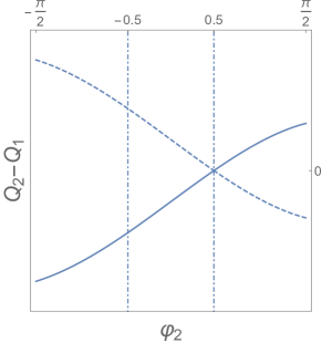
Figure 5: Josephson curve given by Eq. (69) for $\varphi_{1}=.5$. The solid curve represents the shocks moving to the right, the dashed – to the left.

Appendix C Riemann method of characteristics

Multiplying (15a) by $\pm\sqrt{\cos\varphi}$ and adding to (15b) we obtain

$$\frac{\partial Q}{\partial\tau}+\sqrt{\cos\varphi}\frac{\partial\varphi}{\partial\tau}+\sqrt{\cos\varphi}\left(\frac{\partial Q}{\partial Z}+\sqrt{\cos\varphi}\frac{\partial\varphi}{\partial Z}\right) =0.$$ (70a)

$$\frac{\partial Q}{\partial\tau}-\sqrt{\cos\varphi}\frac{\partial\varphi}{\partial\tau}-\sqrt{\cos\varphi}\left(\frac{\partial Q}{\partial Z}-\sqrt{\cos\varphi}\frac{\partial\varphi}{\partial Z}\right) =0.$$ (70b)

After we introduce the new variables

$$J_{+} =\int\sqrt{\cos\varphi}d\varphi+Q,$$ (71a)

$$J_{-} =\int\sqrt{\cos\varphi}d\varphi-Q,$$ (71b)

called the Riemann invariants Eq. (70) takes the form

$$\left(\frac{\partial}{\partial\tau}+\sqrt{\cos\varphi}\frac{\partial}{\partial Z}\right)J_{+} =0,$$ (72a)

$$\left(\frac{\partial}{\partial\tau}-\sqrt{\cos\varphi}\frac{\partial}{\partial Z}\right)J_{-} =0,$$ (72b)

where $\varphi$ should be understood as the function of $J_{+}$ and $J_{-}$ obtained by solving (71). Note that the differential operators acting on $J_{+}$ and $J_{-}$ are just the operators of differentiation along the characteristics

$$C_{+/-}:\frac{dZ}{d\tau} =\pm\sqrt{\cos\varphi}$$ (73)

in the $Z\tau$-plane. Thus we see that $J_{+}$ and $J_{-}$ remain constant along each characteristic $C_{+}$ or $C_{-}$ respectively. We can also say that small perturbations of $J_{+}$ are propagated only along the characteristics C+, and those of $J_{-}$ only along $C_{-}$ landau2 .

References

- (1) G. B. Whitham, Linear and Nonlinear Waves, John Wiley & Sons Inc., New York (1999).
- (2) D. M. French and B. W. Hoff, IEEE Trans. Plasma Sci. 42, 3387 (2014).
- (3) B. Nouri, M. S. Nakhla, and R. Achar, IEEE Trans. Microw. Theory Techn. 65, 673 (2017).
- (4) L. P. S. Neto, J. O. Rossi, J. J. Barroso, and E. Schamiloglu, IEEE Trans. Plasma Sci. 46, 3648 (2018).
- (5) M. S. Nikoo, S. M.-A. Hashemi, and F. Farzaneh, IEEE Trans. Microw. Theory Techn. 66, 3234 (2018); 66, 4757 (2018).
- (6) L. C. Silva, J. O. Rossi, E. G. L. Rangel, L. R. Raimundi, and E. Schamiloglu, Int. J. Adv. Eng. Res. Sci. 5, 121 (2018).
- (7) Y. Wang, L.-J. Lang, C. H. Lee, B. Zhang, and Y. D. Chong, Nat. Comm. 10, 1102 (2019).
- (8) E. G. L. Range, J. O. Rossi, J. J. Barroso, F. S. Yamasaki, and E. Schamiloglu, IEEE Trans. Plasma Sci. 47, 1000 (2019).
- (9) A. S. Kyuregyan, Semiconductors 53, 511 (2019).
- (10) N. A. Akem, A. M. Dikande, and B. Z. Essimbi, SN Applied Science 2, 21 (2020).
- (11) A. J. Fairbanks, A. M. Darr, A. L. Garner, IEEE Access 8, 148606 (2020).
- (12) R. Landauer, IBM J. Res. Develop. 4, 391 (1960).
- (13) S. T. Peng and R. Landauer, IBM J. Res. Develop. 17(1973).
- (14) M. I. Rabinovich and D. I. Trubetskov, Oscillations and Waves, Kluwer Academic Publishers, Dordrecht / Boston / London (1989).
- (15) A. Barone and G. Paterno, Physics and Applications of the Josephson Effect, John Wiley & Sons, Inc, New York (1982).
- (16) N. F. Pedersen, Solitons in Josephson Transmission lines, in Solitons, North-Holland Physics Publishing, Amsterda (1986).
- (17) C. Giovanella and M. Tinkham, Macroscopic Quantum Phenomena and Coherence in Superconducting Networks, World Scientific, Frascati (1995).
- (18) A. M. Kadin, Introduction to Superconducting Circuits, Wiley and Sons, New York (1999).
- (19) M. Remoissenet, Waves Called Solitons: Concepts and Experiments, Springer-Verlag Berlin Heidelberg GmbH (1996).
- (20) O. Yaakobi, L. Friedland, C. Macklin, and I. Siddiqi, Phys. Rev. B 87, 144301 (2013).
- (21) K. O’Brien, C. Macklin, I. Siddiqi, and X. Zhang, Phys. Rev. Lett. 113, 157001 (2014).
- (22) C. Macklin, K. O’Brien, D. Hover, M. E. Schwartz, V. Bolkhovsky, X. Zhang, W. D. Oliver, and I. Siddiqi, Science 350, 307 (2015).
- (23) B. A. Kochetov, and A. Fedorov, Phys. Rev. B. 92, 224304 (2015).
- (24) A. B. Zorin, Phys. Rev. Applied 6, 034006 (2016); Phys. Rev. Applied 12, 044051 (2019).
- (25) D. M. Basko, F. Pfeiffer, P. Adamus, M. Holzmann, and F. W. J. Hekking, Phys. Rev. B 101, 024518 (2020).
- (26) T. Dixon, J. W. Dunstan, G. B. Long, J. M. Williams, Ph. J. Meeson, C. D. Shelly, Phys. Rev. Applied 14, 034058 (2020)
- (27) A. Burshtein, R. Kuzmin, V. E. Manucharyan, and M. Goldstein, Phys. Rev. Lett. 126, 137701 (2021).
- (28) T. C. White et al., Appl. Phys. Lett. 106, 242601 (2015).
- (29) A. Miano and O. A. Mukhanov, IEEE Trans. Appl. Supercond. 29, 1501706 (2019).
- (30) Ch. Liu, Tzu-Chiao Chien, M. Hatridge, D. Pekker, Phys. Rev. A 101, 042323 (2020).
- (31) P. Rosenau, Phys. Lett. A 118, 222 (1986); Phys. Scripta 34, 827 (1986).
- (32) G. J. Chen and M. R. Beasley, IEEE Trans. Appl. Supercond. 1, 140 (1991).
- (33) H. R. Mohebbi and A. H. Majedi, IEEE Trans. Appl. Supercond. 19, 891 (2009); IEEE Transactions on Microwave Theory and Techniques 57, 1865 (2009).
- (34) D. S. Ricketts and D. Ham, Electrical Solitons: Theory, Design, and Applications, CRC Press (2018).
- (35) A. Houwe, S. Abbagari, M. Inc, G. Betchewe, S. Y. Doka, K. T. Crepin, and K. S. Nisar, Results in Physics 18, 103188 (2020).
- (36) H. Katayama, N. Hatakenaka, and T. Fujii, Phys. Rev. D 102, 086018 (2020).
- (37) D. L. Sekulic, N. M. Samardzic, Z. Mihajlovic, and M. V. Sataric, Electronics 10, 2278 (2021).
- (38) P. G. Kevrekidis, I. G. Kevrekidis, A. R. Bishop, and E. Titi, Phys. Rev. E, 65, 046613 (2002).
- (39) L. Q. English, F. Palmero, A. J. Sievers, P. G. Kevrekidis, and D. H. Barnak, Phys. Rev. E, 81, 046605 (2010).
- (40) P. G. Kevrekidis, IMA Journal of Applied Mathematics 76, 389 (2011)
- (41) V. Nesterenko, Dynamics of heterogeneous materials, Springer Science & Business Media (2013).
- (42) B. A. Malomed, The sine-gordon model: General background, physical motivations, inverse scattering, and solitons, The Sine-Gordon Model and Its Applications. Springer, Cham, 1-30 (2014).
- (43) V. F. Nesterenko, Phil. Trans. R. Soc. A 376, 20170130 (2018).
- (44) B. A. Malomed, Nonlinearity and discreteness: Solitons in lattices, Emerging Frontiers in Nonlinear Science. Springer, Cham, 81 (2020).
- (45) E. Kengne, Wu-Ming Liu, L. Q. English, and B. A. Malomed, Phys. Rep. 982, 1 (2022).
- (46) E. Kogan, Journal of Applied Physics 130, 013903 (2021).
- (47) E. Kogan, physica status solidi (b), 259, 2200160 (2022).
- (48) L. D. Landau and E. M. Lifshitz, Fluid Mechanics, Pergamonn Press, 1987.
- (49) E. Kogan, Phys. Stat. Sol. (b), 2200403 (2022).
- (50) A. M. Kamchatnov, Nonlinear Periodic waves and Their Modulations, World Scientific Publishing, Singapore, 2000.
- (51) G. Gallavotti, ed. The Fermi-Pasta-Ulam problem: a status report, Vol. 728. Springer, 2007.