Noether Symmetries and Some Exact Solutions in $f(R,T^{2})$ Theory

Abstract

The main objective of this article is to examine some physically viable solutions through the Noether symmetry technique in $f(R,T^{2})$ theory. For this purpose, we assume a generalized anisotropic and homogenous spacetime that yields distinct cosmic models. In order to investigate Noether equations, symmetry generators and conserved quantities, we use a specific model of this modified theory. We find exact solutions and examine the behavior of various cosmological quantities. It is found the behavior these quantities is consistent with current observations indicating that this theory describes the cosmic accelerated expansion. We conclude that generators of Noether symmetry and conserved quantities exist in this theory.

1 Introduction

The current cosmic expansion has been the most stunning and dazzling result for the scientific community [1]. Although general relativity (GR) is a widely accepted theory which explains the cause of this expansion but it has some issues like coincidence and fine tuning problems. To addresses these issues, several modifications of GR (modified gravitational theories) have been formulated to unveil the cosmic mysteries. The first modification of GR is $f(R)$ theory and significant literature [2] is available to understand the physical features of this theory. Nojiri and Odinstov [3] The minimal coupled theory was established in [4] named as $f(G,T)$ theory while $f(R,T,R_{\xi\eta}T^{\xi\eta})$ is a non-minimal coupled theory [5].

Nojiri and Odintsov [6] reviewed various modified gravitational theories such as $f(R)$, $f(G)$ and $f(R,G)$ gravity models which are assumed as alternative theories for dark energy. They showed that some of such theories may pass the solar system tests and have quite rich cosmological structure: they may naturally describe the effective (cosmological constant, quintessence or phantom) with a possible transition from deceleration to acceleration era. The possibility to explain the coincidence problem as the manifestation of the universe expansion in such models is mentioned. The late (phantom or quintessence) universe filled with dark fluid with inhomogeneous equation of state (where inhomogeneous terms are originated from the modified gravity) is also described.

Nojiri et al [7] discussed some standard issues and also the latest developments of modified theories in cosmology, emphasizing on inflation, bouncing cosmology and late-time acceleration era. In particular, they presented the formalism of $f(R)$, $f(G)$ and $f(T)$ gravity theories. They emphasized on the formalism of these theories and explained how these theories can be considered as viable descriptions for our universe. They demonstrated how bouncing cosmology can actually be described by these theories. Moreover, they discussed several qualitative features of the dark energy era by using the modified gravity formalism and also discussed how a unified description of inflation with dark energy era can be described by using the modified gravity framework. They also discussed some astrophysical solutions in the context of modified gravity and several qualitative features of these solutions. Capozziello and Laurentis [8] examined that extended theories of gravity can be considered a new paradigm to cure shortcomings of GR at infrared and ultraviolet scales. They focused on specific classes of theories like $f(R)$ gravity, scalar-tensor gravity in the metric and Palatini approaches. A number of viability criteria are presented considering the post-Newtonian and the post Minkowskian limits. In particular, they discussed the problems of neutrino oscillations and gravitational waves in extended gravity.

Recently, Katirci and Kavuk [9] modified $f(R)$ theory by introducing a non-linear term $(T^{2}=T_{\xi\eta}T^{\xi\eta})$ in the functional action referred to as $f(R,T^{2})$ theory. This curvature-matter coupled theory develops a particular relation between geometry and matter which provides a more comprehensive description to unveil the dark components of the universe. This proposal is also dubbed as energy-momentum squared gravity (EMSG) and contains higher-order matter source terms which are helpful to analyze various interesting cosmological results. It is worthwhile to mention here that this theory explains the complete cosmic history and the cosmic evolution. Roshan and Shojai [10] examined that EMSG resolves the primordial singularity as it has bounce in the early universe. Board and Barrow [11] used a specific model of this theory and discussed exact solution, singularities as well as cosmic evolution with the isotropic configuration of matter in this theory. Bahamonde et al [12] studied various EMSG models and analyzed that these models manifest the current cosmic evolution and acceleration. Ranjit et al [13] examined possible solutions for matter density and discussed their cosmological results in EMSG. We have examined some physically viable solutions in this theory [14]. We have also studied the dynamics of celestial objects and found that collapse rate reduces in EMSG as compared to GR [15]. Recently, Sharif and Naz [16] studied physical characteristics of a gravastar in this framework.

The universe is homogeneous and isotropic at large scales according to the cosmic observations such as Planck satellites and Cosmic microwave background. But, the cosmos was found to be anisotropic and spatially homogeneous in the past times. The Cosmic microwave background temperature is used as anisotropy in the current universe. Bianchi type (BT) spacetimes are the most important and elegant models that determine the effect of anisotropy in the early time, i.e., the less anisotropy stops the rapid cosmic expansion that yields a highly isotropic universe [17]. Several researchers have analyzed these models in a different context. The BT-I model with anisotropic matter has been studied in [18] and investigated that the effective density and EoS parameter describes the cosmic expansion. The BT-I model with the dominance of DE has been investigated in [19] and they examined that DE is responsible for cosmic expansion. The exact anisotropic solutions in curvature-matter coupled theory has been studied in [20].

The features of a mathematical or physical system that do not change due to some change are determined by symmetry. Exact solutions of non-linear differential equations have been formulated in a significant way using symmetry approaches. Symmetry at geometric level occurs when a system maintains its shape after going through particular transformations like rotation, reflection or scaling. Continuous symmetry appears because of continuous change in the system such as Noether symmetry (NS) that corresponds to the Lagrangian. The feasible characteristics of the system can be discussed by defining the Lagrangian which describes energy content and gives knowledge about the symmetries exist in the system. However, the most efficient method for establishing a connection between generators and the system’s conserved values is NS technique [21]. This approach simplifies the system and offers new solutions for deciphering the mysterious cosmos.

The NS approach is significant as it recovers symmetry generators as well as some conservation laws of the system [22]. This method does not deal only with the dynamical solutions but it also provides some viable conditions to select cosmic models based on recent observations [23]. Moreover, this method is an important and useful technique to examine exact solutions by using conserved values of the system. Conservation laws are the main ingredients to analyze the distinct physical phenomena. These are the particular cases of the Noether theorem, according to which every differentiable symmetry produces conservation laws. The conservation laws of linear and angular momentum govern the translational and rotational symmetry of any object. The Noether charges are important in the literature as they are used to examine various major cosmic problems in various considerations [24]-[34]. Exact solutions of the spherical spacetime through NS in $f(R)$ theory has been obtained in [35]. The stability of spherical and FRW universe models in the same theory has been investigated in [36]. Kucukakca et al [37] found analytic solutions for various universe models in the scalar-tensor theory. In the framework of $f(R,T)$ theory, the exact viable solutions has been examined in [38]. Recently, we have analyzed stable modes of Einstein universe [39] and the geometry of celestial objects in EMSG [40].

This manuscript investigates the NS for anisotropic and homogenous cosmic models such as BT-I, BT-III and Kantowski-Sachs (KS) in the background of EMSG. We analyze generators of the NS with conserved quantities and evaluate cosmological solutions for a specific EMSG model to investigate the cosmic evolution. The format of this manuscript is planned as follows. Section 2 studies the basic formalism of EMSG. Section 3 provides a detailed study of the NS approach and derives exact cosmological solutions which are then discussed through graphs. The summary of the consequences is given in section 4.

2 Field Equations

We derive the field equations of the homogeneous and anisotropic spacetime in this section. The action of EMSG is expressed as [4]

$$A=\int\left(\frac{f(R,T^{2})}{2\kappa^{2}}+L_{m}\right)d^{4}x\sqrt{-g},$$ (1)

where $\kappa^{2}=1$ and $\mathcal{L}_{m}$ manifest the coupling constant and Lagrangian of matter, respectively. The corresponding equations of motion are obtained as

$$R_{\xi\eta}f_{R}+g_{\xi\eta}\Box f_{R}-\nabla_{\xi}\nabla_{\eta}f_{R}-\frac{1}{2}g_{\xi\eta}f=T_{\xi\eta}-\Theta_{\xi\eta}f_{T^{2}},$$ (2)

where $\Box=\nabla_{\xi}\nabla^{\xi},~{}f_{T^{2}}=\frac{\partial f}{\partial T^{2}},~{}f_{R}=\frac{\partial f}{\partial R}$ and

$$\Theta_{\xi\eta}=-2L_{m}(T_{\xi\eta}-\frac{1}{2}g_{\xi\eta}T)-4\frac{\partial^{2}L_{m}}{\partial g^{\xi\eta}\partial g^{\alpha\beta}}T^{\alpha\beta}-TT_{\xi\eta}+2T_{\xi}^{\alpha}T_{\eta\alpha}.$$

Rearranging Eq.(2), we have

$$G_{\xi\eta}=\frac{1}{f_{R}}(T_{\xi\eta}^{(D)}+T_{\xi\eta})=T_{\xi\eta}^{eff},$$ (3)

where $T_{\xi\eta}=(\rho+p)U_{\xi}U_{\eta}+pg_{\xi\eta}$ and $T_{\xi\eta}^{(D)}$ defines the modified terms of EMSG, represented as

$$T_{\xi\eta}^{(D)}=\frac{1}{2}g_{\xi\eta}(f-Rf_{R})-g_{\xi\eta}\Box f_{R}+\nabla_{\xi}\nabla_{\eta}f_{R}-\Theta_{\xi\eta}f_{T^{2}}.$$ (4)

We assume a generalized spacetime that corresponds to BT-I, BT-III and KS spacetimes as

$$ds^{2}=-dt^{2}+a^{2}(t)dx^{2}+b^{2}(t)(d\theta^{2}+\psi^{2}(\theta)d\phi^{2}),$$ (5)

where $\psi(\theta)=\theta,~{}\sinh\theta,~{}\sin\theta$ satisfying the relation

$$\frac{1}{\psi}\frac{d^{2}\psi}{d\theta^{2}}=-\epsilon.$$

For $\epsilon=0,-1,1$, the BT-I, BT-III and KS cosmic models are obtained. The resulting equations of motion become

$$\rho^{eff} = \frac{1}{f_{R}}[\rho-\frac{1}{2}f+(3p^{2}+\rho^{2}+4p\rho)f_{T^{2}}+\epsilon b^{-2}f_{R}-(\dot{a}a^{-1}+2\dot{b}b^{-1})$$ (6)

$$\times (\dot{R}f_{RR}+\dot{T}^{2}f_{RT^{2}})+(\ddot{a}a^{-1}+2\ddot{b}b^{-1}+2\dot{a}\dot{b}a^{-1}b^{-1}+\dot{b}^{2}b^{-2})f_{R}],$$

$$p^{eff} = \frac{1}{f_{R}}[p+\frac{1}{2}f+2\dot{b}b^{-1}(\dot{R}f_{RR}+\dot{T}^{2}f_{RT^{2}})-\epsilon b^{-2}f_{R}+\ddot{R}f_{RR}+\ddot{T}^{2}$$ (7)

$$\times f_{RT^{2}}-(\ddot{a}a^{-1}+2\ddot{b}b^{-1}+2\dot{a}\dot{b}a^{-1}b^{-1}+\dot{b}^{2}b^{-2})f_{R}+\dot{R}^{2}f_{RRR}+\dot{T}^{2}$$

$$\times f_{RT^{2}T^{2}}+2\dot{R}\dot{T}f_{RRT^{2}}],$$

$$p^{eff} = \frac{1}{f_{R}}[p+\frac{1}{2}f+(\dot{a}a^{-1}+\dot{b}b^{-1})(\dot{R}f_{RR}+\dot{T}^{2}f_{RT^{2}})-\epsilon b^{-2}f_{R}+\ddot{T}^{2}$$ (8)

$$\times f_{RT^{2}}+\ddot{R}f_{RR}-(\ddot{a}a^{-1}+2\ddot{b}b^{-1}+2\dot{a}\dot{b}a^{-1}b^{-1}+\dot{b}^{2}b^{-2})f_{R}+\dot{R}^{2}$$

$$\times f_{RRR}+\dot{T}^{2}f_{RT^{2}T^{2}}+2\dot{R}\dot{T}f_{RRT^{2}}],$$

Now, we apply Lagrange multiplier method to formulate the Lagrangian as

$$L = ab^{2}(f-Rf_{R}-T^{2}f_{T^{2}}+(3p^{2}+\rho^{2})f_{T^{2}}+p)-2a(2\dot{a}\dot{b}ba^{-1}$$ (9)

$$+ \dot{b}^{2}-\epsilon)f_{R}-(2b^{2}\dot{a}+4ab\dot{b})\dot{R}f_{RR}-(2b^{2}\dot{a}+4ab\dot{b})\dot{T}^{2}f_{RT^{2}}.$$

The fundamental properties of the system can be explained using the Hamiltonian $(E)$ and the dynamical equations , determined as

$$\frac{\partial L}{\partial q^{i}}-\frac{d}{dt}(\frac{\partial L}{\partial\dot{q}^{i}})=0,\quad E=\dot{q}^{i}(\frac{\partial L}{\partial\dot{q}^{i}})-L,$$ (10)

where generalized coordinates are denoted by $q^{i}$. The resulting dynamical equations are

$$f-Rf_{R}-T^{2}f_{T^{2}}+(3p^{2}+\rho^{2})f_{T^{2}}+p+4\dot{b}b^{-1}(\dot{R}f_{RR}+f_{RT^{2}}$$

$$\times\dot{T}^{2})+a(f_{T^{2}}(6pp_{,a}+2\rho\rho_{,a})+p_{,a})+b^{-2}(2\dot{b}^{2}+4\ddot{b}b+2\epsilon)f_{R}$$

$$+2\ddot{R}f_{RR}+2\ddot{T}^{2}f_{RT^{2}}+2\dot{R}^{2}f_{RRR}+2\dot{T}^{2}f_{RT^{2}T^{2}}+4\dot{R}\dot{T}^{2}f_{RRT^{2}}=0,$$ (11)

$$f-Rf_{R}-T^{2}f_{T^{2}}+(3p^{2}+\rho^{2})f_{T^{2}}+(\dot{R}f_{RR}+\dot{T}^{2}f_{R}T^{2})4\dot{a}a^{-1}$$

$$+p+b(f_{T^{2}}(6pp_{,b}+2\rho\rho_{,b})+p_{,b})+2a^{-1}b^{-1}(\ddot{a}b+\dot{a}\dot{b}+\ddot{b}a)f_{R}$$

$$+2\ddot{f_{R}}+4\dot{b}b^{-1}(\dot{R}f_{RRT^{2}}+\dot{T}^{2}f_{RT^{2}T^{2}})=0,$$ (12)

$$(2\ddot{a}a^{-1}-4\ddot{b}b^{-1})f_{RR}+(3p^{2}+\rho^{2})f_{RT^{2}}-2\epsilon b^{-1}f_{RR}-Rf_{RR}$$

$$-T^{2}f_{RT^{2}}-(4\dot{a}\dot{b}a^{-1}b^{-1}+2\dot{b}^{2}b^{-2})f_{RR}=0,$$ (13)

$$(2\ddot{a}a^{-1}-4\ddot{b}b^{-1})f_{RT^{2}}+(3p^{2}+\rho^{2})f_{T^{2}T^{2}}-2\epsilon b^{-1}f_{RT^{2}}-Rf_{RT^{2}}$$

$$-T^{2}f_{T^{2}T^{2}}-(4\dot{a}\dot{b}a^{-1}b^{-1}+2\dot{b}^{2}b^{-2})f_{RT^{2}}=0.$$ (14)

We formulate the Hamiltonian to examine the total energy of the system as

$$E = -ab^{2}(f-Rf_{R}-T^{2}f_{T^{2}}+(3p^{2}+\rho^{2})f_{T^{2}})-(2\dot{a}\dot{b}ba^{-1}+\dot{b}^{2})$$ (15)

$$\times 2af_{R}-\epsilon f_{R}-ab^{2}p-(2b^{2}\dot{a}+4ab\dot{b})\dot{f_{R}}.$$

The dynamical equations (11)-(14) are extremely complex due to metavariable functions and their derivatives. Despite being very challenging to solve these equations directly, these can be solved in one of two ways. The first is numerically or analytically approach, and the second is NS technique to identify exact solutions. Although this theory is not conserved but one can obtain conserved values through NS approach, which are then used to examine the mysterious universe. As a result, latter strategy because it is more intriguing. Thus, we will employ the later approach as it is more interesting.

3 Noether Symmetries in EMSG

The NS strategy gives a fascinating method to develop new cosmic models and associated structures in modified theories of gravity. This section formulates the Noether equations for the homogenous and anisotropic universe model in EMSG. This approach establishes a vector field that corresponds to tangent space. Thus, the vector field acts as a generator and gives conserved quantities that can be used to analyze viable solutions. The symmetry generators are expressed as

$$Y=\lambda(t,q^{i})\frac{\partial}{\partial t}+\Upsilon^{j}(t,q^{i})\frac{\partial}{\partial q^{j}},\quad i=1,2,3...,n,$$

where $\lambda(t,a,b,R,T^{2})$ and $\Upsilon^{j}(t,a,b,R,T^{2})$ are the unknown parameters. In our case, the Lagrangian admits five degrees of freedom and hence the symmetry generator becomes

$$Y=\lambda\frac{\partial}{\partial t}+\Upsilon^{1}\frac{\partial}{\partial a}+\Upsilon^{2}\frac{\partial}{\partial b}+\Upsilon^{3}\frac{\partial}{\partial R}+\Upsilon^{4}\frac{\partial}{\partial T^{2}}.$$ (16)

The Lagrangian must satisfy the invariance constraint, expressed as

$$Y^{[1]}L+(D\lambda)L=D\Omega,\quad Y^{[1]}=Y+\dot{\Upsilon}^{i}\frac{\partial}{\partial\dot{q}^{i}}$$ (17)

where $\Omega$ is the boundary term and $D=\frac{\partial}{\partial t}+\dot{q}^{i}\frac{\partial}{\partial q^{i}}$ defines the total derivative. The corresponding integral integral of motion is expressed as

$$I=\Upsilon^{i}\frac{\partial L}{\partial\dot{q}^{i}}-\lambda E-\Omega.$$ (18)

This is a crucial component of NS that is essential for computing viable solutions and is also named as the conserved quantities.

We take the vector field $(Y)$ with configuration space $Q=({t,a,b,R,T^{2}})$ to examine the generators with corresponding first integrals of Lagrangian (9) under invariance condition (17). By comparing the coefficients of Eq.(17), we have

$$2b^{2}\Upsilon^{1}_{,t}f_{RT^{2}}+4ab\Upsilon^{2}_{,t}f_{RT^{2}}+\Omega_{,T^{2}}=0,$$ (19)

$$2b^{2}\Upsilon^{1}_{,t}f_{RR}+4ab\Upsilon^{2}_{,t}f_{RR}+\Omega_{,R}=0,\quad\lambda_{,a}f_{R}=0,$$ (20)

$$b\Upsilon^{1}_{,T^{2}}f_{RR}+b\Upsilon^{1}_{,R}f_{RT^{2}}+2a\Upsilon^{2}_{,T^{2}}f_{RR}+2a\Upsilon^{2}_{,R}f_{RT^{2}}=0,$$ (21)

$$4b\Upsilon^{1}_{,t}f_{R}+4a\Upsilon^{2}_{,t}f_{R}+4ab\Upsilon^{3}_{,t}f_{RR}+4ab\Upsilon^{4}_{,t}f_{RT^{2}}+\Omega_{,b}=0,$$ (22)

$$4b\Upsilon^{2}_{,t}f_{R}+2b^{2}\Upsilon^{3}_{,t}f_{RR}+2b^{2}\Upsilon^{4}_{,t}f_{RT^{2}}+\Omega_{,a}=0,\quad\lambda_{,b}f_{R}=0,$$ (23)

$$b\Upsilon^{1}_{,T^{2}}f_{RR}+2ab\Upsilon^{2}_{,T^{2}}f_{RT^{2}}=0,\quad\lambda_{,R}f_{RR}=0,\quad\lambda_{,T^{2}}f_{RT^{2}}=0,$$ (24)

$$b\Upsilon^{1}_{,R}f_{RR}+2ab\Upsilon^{2}_{,R}f_{RR}=0,\quad 2\Upsilon^{2}_{,a}f_{R}+b\Upsilon^{3}_{,a}f_{RR}+b\Upsilon^{4}_{,a}f_{RT^{2}}=0,$$ (25)

$$\Upsilon^{1}f_{R}+a\Upsilon^{3}f_{RR}+a\Upsilon^{4}f_{RT^{2}}+2b\Upsilon^{1}_{,b}f_{R}+2ab\Upsilon^{4}_{,b}f_{RT^{2}}+2ab\Upsilon^{3}_{,b}f_{RR}$$

$$-a\lambda_{,t}f_{R}+2a\Upsilon^{2}_{,b}f_{R}=0,\quad\lambda_{,a}f_{RR}=0,\quad\lambda_{,a}f_{RT^{2}}=0,$$ (26)

$$+2\Upsilon^{2}_{,R}f_{R}+b\Upsilon^{3}_{,R}f_{RR}+b\Upsilon^{4}_{,R}f_{RT^{2}}-b\lambda_{,t}f_{RR}+2\Upsilon^{2}f_{RR}+b\Upsilon^{1}_{,a}f_{RR}$$

$$+b\Upsilon^{3}f_{RRR}+b\Upsilon^{4}f_{RRT^{2}}+2a\Upsilon^{2}_{,a}f_{RR}=0,\quad\lambda_{,b}f_{RR}=0,$$ (27)

$$2\Upsilon^{2}f_{RT^{2}}-b\lambda_{,t}f_{RT^{2}}+b\Upsilon^{3}_{,T^{2}}f_{RR}+b\Upsilon^{1}_{,a}f_{RT^{2}}+b\Upsilon^{4}_{,T^{2}}f_{RT^{2}}+2\Upsilon^{2}_{,T^{2}}f_{R}$$

$$+b\Upsilon^{4}f_{RT^{2}T^{2}}+2a\Upsilon^{2}_{,a}f_{RT^{2}}+b\Upsilon^{3}f_{RRT^{2}}=0,\quad\lambda_{,b}f_{RT^{2}}=0,$$ (28)

$$2\Upsilon^{2}f_{R}+2b\Upsilon^{3}f_{RR}+2b\Upsilon^{4}f_{RT^{2}}+2b\Upsilon^{1}_{,a}f_{R}+2a\Upsilon^{2}_{,a}f_{R}+2ab\Upsilon^{3}_{,a}f_{RR}$$

$$+2b\Upsilon^{2}_{,T^{2}}f_{R}+b^{2}\Upsilon^{3}_{,b}f_{RR}+2ab\Upsilon^{4}_{,a}f_{RT^{2}}+b^{2}\Upsilon^{4}_{,b}f_{RT^{2}}-2b\lambda_{,t}f_{R}=0,$$ (29)

$$2b\Upsilon^{1}f_{RR}+2a\Upsilon^{2}f_{RR}+2ab\Upsilon^{3}f_{RRR}+2ab\Upsilon^{4}f_{RRT^{2}}+b^{2}\Upsilon^{1}_{,b}f_{RR}$$

$$+2b\Upsilon^{1}_{,R}f_{R}+2ab\Upsilon^{2}_{,b}f_{RR}+2a\Upsilon^{2}_{,R}f_{R}+2ab\Upsilon^{3}_{,R}f_{RR}+2ab\Upsilon^{4}_{,R}f_{RT^{2}}$$

$$-2ab\lambda_{,t}f_{RR}=0,\quad\lambda_{,R}f_{R}=0,\quad\lambda_{,T^{2}}f_{R}=0,$$ (30)

$$2b\Upsilon^{1}f_{RT^{2}}+2a\Upsilon^{2}f_{RT^{2}}+2ab\Upsilon^{3}f_{RRT^{2}}+2ab\Upsilon^{4}f_{RT^{2}T^{2}}+b^{2}\Upsilon^{1}_{,b}f_{RT^{2}}$$

$$+2b\Upsilon^{1}_{,T^{2}}f_{R}+2ab\Upsilon^{2}_{,b}f_{RT^{2}}+2a\Upsilon^{2}_{,T^{2}}f_{R}+2ab\Upsilon^{3}_{,T^{2}}f_{RR}+2ab\Upsilon^{4}_{,T^{2}}f_{RT^{2}}$$

$$-2ab\lambda_{,t}f_{RT^{2}}=0,\quad\lambda_{,R}f_{RT^{2}}=0,\quad\lambda_{,T^{2}}f_{RR}=0,$$ (31)

$$b^{2}\Upsilon^{1}[f-Rf_{R}-T^{2}f_{T^{2}}+(3p^{2}+\rho^{2})f_{T^{2}}+p+a((6pp_{,a}+2\rho\rho_{,a})f_{T^{2}}$$

$$+p_{,a})+2\epsilon f_{R}]+\Upsilon^{2}[2ab(f-Rf_{R}-T^{2}f_{T^{2}}+(3p^{2}+\rho^{2})f_{T^{2}}+p)$$

$$+ab^{2}((6pp_{,b}+2\rho\rho_{,b})f_{T^{2}}+p_{,b})]+(3p^{2}+\rho^{2})f_{RT^{2}})+\Upsilon^{3}[-ab^{2}(Rf_{RR}$$

$$-T^{2}f_{RT^{2}}+(3p^{2}+\rho^{2})f_{T^{2}T^{2}})+2a\epsilon f_{RR}]+\Upsilon^{4}[-ab^{2}(Rf_{RT^{2}}-T^{2}f_{T^{2}T^{2}}$$

$$-(3p^{2}+\rho^{2})f_{T^{2}T^{2}})+2a\epsilon f_{RT^{2}}]+\lambda_{,t}[ab^{2}(f-Rf_{R}-T^{2}f_{T^{2}}+2\epsilon f_{R}$$

$$+(3p^{2}+\rho^{2})f_{T^{2}}+p)]-\Omega_{,t}=0.$$ (32)

These equations help to study the dark cosmos in the context of $f(R,T^{2})$. We solve the above system to obtain exact solutions for specific $f(R,T^{2})$ model in the following section.

3.1 Exact Solutions

Here, we formulate the generators of NS, conserved values of the system and corresponding physical solutions. Due to the above system’s complexity and nonlinearity, we assume a particular EMSG model $f(R,T^{2})=R+T^{2}$ which minimizes the system complexity and help to examine the exact solutions [5]. Manipulating Eqs.(19)-(32), we obtain

$$\Upsilon^{1} = \frac{1}{3}a\dot{F_{1}}(t)-2c_{1}a-\frac{1}{2}\frac{aF_{2}(t)}{b^{\frac{3}{2}}}-\frac{3}{8}\frac{F_{4}(t)}{\sqrt{b}}+\frac{c_{2}}{\sqrt{b}},$$

$$\Upsilon^{2} = \frac{F_{2}(t)}{\sqrt{b}}+(\frac{1}{3}\dot{F_{1}}(t)+c_{1})b,\quad\lambda=F_{1}(t),$$

$$\Psi = -\frac{4}{3}ab^{2}\ddot{F_{1}}(t)-4a\sqrt{b}\dot{F_{2}}(t)+F_{3}(t)+\dot{F_{4}}(t)b^{\frac{3}{2}},$$

$$\rho = \frac{\sqrt{3c_{1}(-3c_{1}a^{2}\epsilon-6c_{1}a\epsilon-2c_{3}at)}}{3c_{1}ba},$$ (33)

where $c_{i}(i=1,...,5)$ are integration constants with $c_{1}\neq 0$. The corresponding symmetry generators become

$$Y_{1}=-3t\frac{\partial}{\partial t},\quad Y_{2}=-3a\frac{\partial}{\partial a}.$$

Substituting the value of Lagrangian (9), Hamiltonian (15) and above solutions (33) in Eq.(18), we obtain first integral as

$$I=12ab\dot{b}c_{1}+3\bigg{[}\frac{3c_{1}a^{2}\epsilon+6c_{1}a\epsilon+2c_{3}at}{3c_{1}a}-2a\dot{b}^{2}-4\dot{a}\dot{b}b+2\frac{\epsilon}{b^{2}}\bigg{]}c_{1}t-c_{3}t^{2}.$$

By comparing the coefficients of $c_{1}$ and $c_{3}$, we have

$$I_{1}=t^{2},\quad I_{2} = 12ab\dot{b}+3t(\epsilon a-2a\dot{b}^{2}-4\dot{a}\dot{b}b+\frac{2\epsilon}{b^{2}}).$$

We substitute Eqs.(33) into dynamical equations (11)-(15) and obtain the exact solution as

$$a(t) = \frac{6c_{5}c_{3}(c_{5}+t)^{\frac{2}{3}}-15c_{1}\epsilon(c_{5}+t)^{\frac{2}{3}}-4c_{3}t(c_{5}+t)^{\frac{2}{3}}+60c_{4}c_{1}\epsilon}{60c_{1}\epsilon(c_{5}+t)^{\frac{2}{3}}},$$

$$b(t) = \frac{1}{2}\sqrt{-6\epsilon}(c_{5}+t).$$ (34)

To analyze this solution, we study the graphical behavior of some important cosmological parameters like deceleration and $r-s$ parameters that are the major factors in the field of cosmology. The Hubble parameter $(H)$ defines the cosmic expansion rate that how quickly it is expanding. The deceleration parameter $(q)$ evaluates the behavior of cosmic expansion. These cosmic parameters for anisotropic and homogeneous universe model are defined as

$$H=\frac{1}{3}(\frac{\dot{a}}{a}+2\frac{\dot{b}}{b}),\quad q=-\frac{H}{H^{2}}-1.$$

The values of these cosmological parameters become

$$H = \frac{2}{3}\bigg{[}4c_{5}c_{3}(c_{5}+t)^{\frac{2}{3}}-15(c_{5}+t)^{\frac{2}{3}}c_{1}\epsilon-6c_{3}t(c_{5}+t)^{\frac{2}{3}}+40c_{4}c_{1}\epsilon\bigg{]}$$

$$\times \bigg{[}(6c_{5}c_{3}(c_{5}+t)^{\frac{2}{3}}-15(c_{5}+t)^{\frac{2}{3}}c_{1}\epsilon-4c_{3}t(c_{5}+t)^{\frac{2}{3}}+60c_{4}c_{1}\epsilon)(c_{5}+t)\bigg{]}^{-1},$$

$$q = \frac{25}{2}\bigg{[}160c_{4}^{2}c_{1}^{2}\sqrt[3]{c_{5}+t}\epsilon^{2}+4c_{5}^{3}c_{3}^{2}(c_{5}+t)^{\frac{2}{3}}-12c_{5}^{2}c_{1}c_{3}(c_{5}+t)^{\frac{2}{3}}\epsilon+4c_{5}^{2}c_{3}^{2}$$

$$\times (c_{5}+t)^{\frac{2}{3}}t+9c_{1}^{2}(c_{5}+t)^{\frac{2}{3}}\epsilon^{2}c_{5}-12c_{5}c_{1}c_{3}(c_{5}+t)^{\frac{2}{3}}\epsilon t+9c_{1}^{2}(c_{5}+t)^{\frac{2}{3}}\epsilon^{2}t$$

$$+ 56c_{4}c_{5}^{2}c_{1}c_{3}\epsilon-60c_{4}c_{5}c_{1}^{2}\epsilon^{2}+72c_{4}c_{5}c_{1}c_{3}\epsilon t-60c_{4}c_{1}^{2}\epsilon^{2}t+16c_{4}c_{1}c_{3}\epsilon t^{2}\bigg{]}$$

$$\times \bigg{[}(4c_{5}c_{3}(c_{5}+t)^{\frac{2}{3}}-15(c_{5}+t)^{\frac{2}{3}}c_{1}\epsilon-6c_{3}t(c_{5}+t)^{\frac{2}{3}}+40c_{4}c_{1}\epsilon)^{2}$$

$$\times \sqrt[3]{c_{5}+t}\bigg{]}^{-1}.$$

The pair of $r-s$ parameters constructs a relationship between formulated and standard models of the universe which is used to examine the characteristics of DE, expressed as

$$r=q+2q^{2}-\frac{\dot{q}}{H},\quad s=\frac{r-1}{3(q-\frac{1}{2})}.$$

For $(r,s)=(1,0)$, the constructed model corresponds to $\Lambda$CDM model whereas quintessence and phantom DE eras are obtained for $s>0$ and $r<1$, respectively. The values of these parameters are bestowed in appendix A. The effective matter variables turn out to be

$$\rho^{eff} = \bigg{[}(6c_{5}c_{3}(c_{5}+t)^{\frac{2}{3}}-15\epsilon c_{1}(c_{5}+t)^{\frac{2}{3}}-4c_{3}t(c_{5}+t)^{\frac{2}{3}}+60c_{4}\epsilon c_{1})(c_{5}+t)^{2}\bigg{]}^{-1}$$

$$\times \bigg{[}\bigg{\{}\frac{1}{\epsilon(c_{5}+t)^{\frac{4}{3}}}(6c_{5}c_{3}(c_{5}+t)^{\frac{2}{3}}-15c_{1}\epsilon(c_{5}+t)^{\frac{2}{3}}-4c_{3}t(c_{5}+t)^{\frac{2}{3}}+60$$

$$\times c_{4}\epsilon c_{1})(2c_{5}c_{3}(c_{5}+t)^{\frac{2}{3}}+35c_{1}\epsilon(c_{5}+t)^{\frac{2}{3}}+12c_{3}t(c_{5}+t)^{\frac{2}{3}}+20c_{4}\epsilon c_{1})\bigg{\}}^{\frac{1}{2}}$$

$$\times \sqrt{-2\epsilon}(c_{5}+t)^{\frac{2}{3}}c_{5}+\bigg{[}\frac{1}{\epsilon(c_{5}+t)^{\frac{4}{3}}}(6c_{5}c_{3}(c_{5}+t)^{\frac{2}{3}}-15\epsilon c_{1}(c_{5}+t)^{\frac{2}{3}}$$

$$- 4c_{3}t(c_{5}+t)^{\frac{2}{3}}+60c_{4}\epsilon c_{1})(2c_{5}c_{3}(c_{5}+t)^{\frac{2}{3}}+35\epsilon c_{1}(c_{5}+t)^{\frac{2}{3}}+20c_{4}\epsilon c_{1}$$

$$+ 12c_{3}t(c_{5}+t)^{\frac{2}{3}})\bigg{]}^{\frac{1}{2}}\sqrt{-2\epsilon}(c_{5}+t)^{\frac{2}{3}}t+2c_{5}c_{3}(c_{5}+t)^{\frac{2}{3}}+35\epsilon c_{1}(c_{5}+t)^{\frac{2}{3}}$$

$$+ 12c_{3}t(c_{5}+t)^{\frac{2}{3}}+20c_{4}\epsilon c_{1}\bigg{]},$$

$$p^{eff} = \bigg{[}2c_{5}c_{3}(c_{5}+t)^{\frac{2}{3}}+35\epsilon c_{1}(c_{5}+t)^{\frac{2}{3}}+12c_{3}t(c_{5}+t)^{\frac{2}{3}}+20c_{4}\epsilon c_{1}\bigg{]}\bigg{[}(6c_{5}c_{3}$$

$$\times (c_{5}+t)^{\frac{2}{3}}-15\epsilon c_{1}(c_{5}+t)^{\frac{2}{3}}-4c_{3}t(c_{5}+t)^{\frac{2}{3}}+60c_{4}\epsilon c_{1})(c_{5}+t)^{2}\bigg{]}^{-1}.$$

The EoS parameter $(\omega^{eff}=\frac{p^{eff}}{\rho^{eff}})$ is a dimensionless quantity that determines the correlation between state parameters. This parameter differentiates the DE era into quintessence $(-1<\omega\leq-1/3)$ and phantom $(\omega<-1)$ phases. This is given as

$$\omega^{eff} = \bigg{[}(2c_{5}c_{3}(c_{5}+t)^{\frac{2}{3}}+35c_{1}\epsilon(c_{5}+t)^{\frac{2}{3}}+12c_{3}t(c_{5}+t)^{\frac{2}{3}}+20c_{4}c_{1}\epsilon)$$

$$\times \bigg{\{}\bigg{[}\frac{1}{\epsilon(c_{5}+t)^{\frac{4}{3}}}\bigg{\{}(6c_{5}c_{3}(c_{5}+t)^{\frac{2}{3}}-15c_{1}\epsilon(c_{5}+t)^{\frac{2}{3}}-4c_{3}t(c_{5}+t)^{\frac{2}{3}}$$

$$+ 60c_{4}c_{1}\epsilon)(2c_{5}c_{3}(c_{5}+t)^{\frac{2}{3}}+35c_{1}\epsilon(c_{5}+t)^{\frac{2}{3}}+12c_{3}t(c_{5}+t)^{\frac{2}{3}}$$

$$+ 20c_{4}c_{1}\epsilon)\bigg{\}}\bigg{]}^{\frac{1}{2}}\sqrt{2}\sqrt{-\epsilon}(c_{5}+t)^{\frac{2}{3}}c_{5}-\bigg{[}\frac{1}{\epsilon(c_{5}+t)^{\frac{4}{3}}}\bigg{\{}(6c_{5}c_{3}(c_{5}+t)^{\frac{2}{3}}$$

$$- 15c_{1}\epsilon(c_{5}+t)^{\frac{2}{3}}-4c_{3}t(c_{5}+t)^{\frac{2}{3}}+60c_{4}c_{1}\epsilon)(2c_{5}c_{3}(c_{5}+t)^{\frac{2}{3}}+35c_{1}\epsilon$$

$$\times (c_{5}+t)^{\frac{2}{3}}+12c_{3}t(c_{5}+t)^{\frac{2}{3}}+20c_{4}c_{1}\epsilon)\bigg{\}}\bigg{]}^{\frac{1}{2}}\sqrt{2}\sqrt{-\epsilon}(c_{5}+t)^{\frac{2}{3}}t$$

$$- 2c_{5}c_{3}(c_{5}+t)^{\frac{2}{3}}-35c_{1}\epsilon(c_{5}+t)^{\frac{2}{3}}-12c_{3}t(c_{5}+t)^{\frac{2}{3}}-20c_{4}c_{1}\epsilon\bigg{\}}^{-1}\bigg{]}.$$

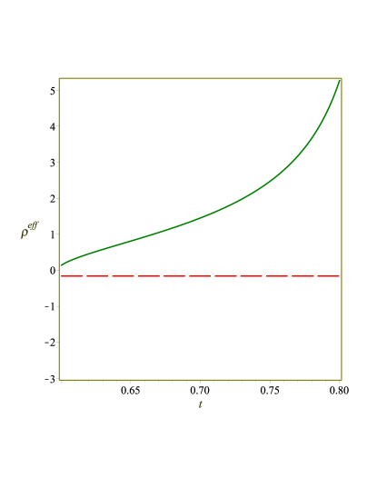
Figure 1: Behavior of effective energy density for $\epsilon=-1$ (line 1) and $\epsilon=1$ (line 2).

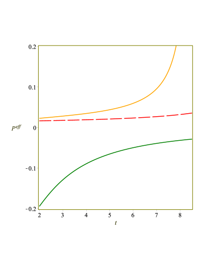
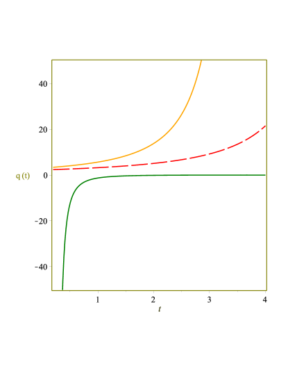
Figure 2: Behavior of effective pressure (Left) and deceleration parameter (Right) for $\epsilon=-1$ (line 1), $\epsilon=1$ (line 2) and $\epsilon=0$ (line 3).

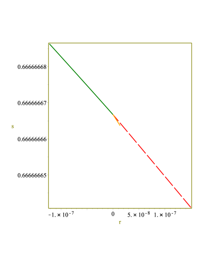
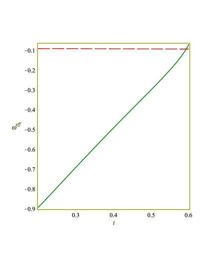
Figure 3: Behavior of $r-s$ (Left) and EoS (Right) parameters for $\epsilon=-1$ (line 1) and $\epsilon=1$ (line 2).

We have considered the values of integration constants as $c_{1}=-2$, $c_{3}=-10$, $c_{4}=10$ and $c_{5}=5.7$ to analyze the graphical behavior of physical quantities. Figure 1 shows that the effective energy density is positively increasing for $\epsilon=-1$ which manifests that our universe is in the expansion phase. Figure 2 shows that the effective pressure and deceleration parameter are negative for BT-III universe model which support the current cosmic acceleration. Figure 3 determines that $r-s$ and EoS parameters describe quintessence and phantom phases of DE which represent the cosmic expansion. The obtained solutions for $\epsilon=-1$ are consistent with recent observations which indicate that this theory demonstrates expansion of the universe.

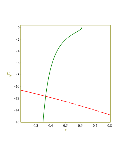
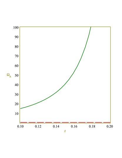
Figure 4: Plot of $\Omega_{m}$ and $\Omega_{\Lambda}$ verses redshift parameter for $\epsilon=-1$ (line 1) and $\epsilon=1$ (line 2).

The total amount of energy density can be expressed as fractional energy density. The fractional density is defined as

$$1+\Omega_{\sigma}=\Omega_{m}+\Omega_{\Lambda},$$

where

$$\Omega_{m}=\frac{\rho}{3H^{2}},\quad\Omega_{\Lambda}=\frac{\rho_{\Lambda}}{3H^{2}},\quad\Omega_{\sigma}=\frac{\sigma^{2}}{3H^{2}}.$$

The evaluation of fractional densities corresponding to ordinary matter $(\Omega_{m})$ and dark energy $(\Omega_{\Lambda})$ plays a vital role to measure the contribution of these elements in the cosmos. The densities for isotropic universe model defined as $\Omega_{m}+\Omega_{\Lambda}=1$ whereas expression equality becomes $\Omega_{m}+\Omega_{\Lambda}=1+\Omega_{\sigma}$ for anisotropic universe model. We analyze the behavior of fractional densities corresponding to matter and dark energy graphically at redshift scale factor where $a(t)=a_{0}(1+z)^{-1}$ and $z$ is the redshift parameter. From observations of Planck data 2018, it is suggested that $\Omega_{m}\cong 0.3111$ and $\Omega_{\Lambda}\cong 0.6889$. According to some recent observations, there are some evidences in favor of closed universe model with fractional density $\Omega_{\Lambda}\cong 0.01$. For $\varepsilon=-1$, the fractional density of matter indicates inconsistent behavior and the trajectory of fractional density provides $\Omega_{m}=0.3$ for $\varepsilon=1$ as shown in Figure 4 (left plot). In this regard, it implies consistent behavior with Planck data 2018. The right plot of Figure 4 reveals the behavior of fractional density of dark energy which shows consistent behavior with Plank data for $\varepsilon=1$ and it exhibits inconsistent behavior for $\varepsilon=-1$.

4 Final Remarks

Modified theories are assumed as the most propitious and elegant proposals to examine the dark universe due to the presence of extra higher-order geometric terms. In this paper, we have formulated exact solutions of anisotropic and homogeneous spacetimes in $f(R,T^{2})$ gravity. For this reason, we have considered the NS technique to examine the exact solutions. We have formulated the Lagrangian, NS generators with conserved values in the background of EMSG. The behavior of exact solutions have been investigated through different cosmological quantities. The main findings are summarized as follows.

• We have established two non-zero NS generators and corresponding conserved quantities. We have obtained the exact solutions for BT-I, BT-III and KS universe models.

• The effective energy density show accelerated and constant expansion corresponding to BT-III, BT-I and KS spacetimes, respectively (Figure 1).

• The value of effective pressure and deceleration parameter remain negative for $\epsilon=-1$ which support the current cosmic acceleration (Figure 2).

• The $r-s$ and EoS parameters yield quintessence and phantom DE phases which determine the rapid expansion of the universe (Figure 3).

• In the background of BT-III universe models, the analysis of fractional density parameter of matter reveals that the EMSG is consistent with Planck 2018 data. In case of KS universe model, this consistency is not preserved (Figure 4). We conclude that the EMSG significantly explains the cosmic journey from decelerated to accelerated epoch.

We find that first integrals of motion are very useful to obtain viable cosmological solutions. It is found that the considered model of EMSG supports the cosmic expansion. Extending this work to the scalar field would be fascinating since it could provide a good foundation for the investigation of the enigmatic cosmos in EMSG.

Appendix A

The values of $r-s$ parameters are

$$r = 25\bigg{[}-126000c_{4}^{2}c_{5}^{2}c_{1}^{3}\epsilon^{3}c_{3}(c_{5}+t)^{\frac{2}{3}}+94800c_{4}^{2}c_{1}^{3}\epsilon^{3}c_{3}t^{2}(c_{5}+t)^{\frac{2}{3}}+7840c_{4}^{2}c_{1}^{2}$$

$$\times c_{3}^{2}\epsilon^{2}t^{3}({c_{5}}+t)^{\frac{2}{3}}+928c_{4}c_{5}^{5}c_{1}\epsilon c_{3}^{3}\sqrt[3]{c_{5}+t}-11520{c_{4}}c_{5}^{4}c_{1}^{2}\epsilon^{2}c_{3}^{2}\sqrt[3]{c_{5}+t}+c_{4}c_{5}^{3}$$

$$\times 34920c_{1}^{3}\epsilon^{3}c_{3}\sqrt[3]{c_{5}+t}-54000c_{4}c_{5}c_{1}^{4}\epsilon^{4}t\sqrt[3]{c_{5}+t}-19080c_{4}c_{1}^{3}c_{3}\epsilon^{3}t^{3}\sqrt[3]{c_{5}+t}$$

$$- 960c_{4}c_{1}^{2}c_{3}^{2}\epsilon^{2}t^{4}\sqrt[3]{c_{5}+t}+34560c_{4}c_{5}^{2}c_{1}^{2}c_{3}^{2}\epsilon^{2}t^{2}\sqrt[3]{c_{5}+t}+1760c_{5}^{2}c_{3}^{3}\epsilon t^{3}\sqrt[3]{c_{5}+t}$$

$$\times c_{4}c_{1}-3240c_{4}c_{5}c_{1}^{3}c_{3}\epsilon^{3}t^{2}\sqrt[3]{c_{5}+t}+21600c_{4}c_{5}c_{1}^{2}c_{3}^{2}\epsilon^{2}t^{3}\sqrt[3]{c_{5}+t}+4480c_{4}c_{1}c_{3}^{3}$$

$$\times c_{5}\epsilon t^{4}\sqrt[3]{c_{5}+t}-29280c_{4}^{2}c_{5}^{2}c_{1}^{2}c_{3}^{2}\epsilon^{2}t(c_{5}+t)^{\frac{2}{3}}-31200c_{4}^{2}c_{5}c_{1}^{3}c_{3}\epsilon^{3}t(c_{5}+t)^{\frac{2}{3}}-c_{1}^{2}$$

$$\times 39680c_{4}^{2}c_{5}c_{3}^{2}\epsilon^{2}t^{2}(c_{5}+t)^{\frac{2}{3}}-3040c_{4}c_{5}^{4}c_{1}c_{3}^{3}\epsilon t\sqrt[3]{c_{5}+t}+480c_{4}c_{5}^{3}c_{1}^{2}c_{3}^{2}\epsilon^{2}t\sqrt[3]{c_{5}+t}$$

$$- 5920c_{4}c_{5}^{3}c_{1}c_{3}^{3}\epsilon t^{2}\sqrt[3]{c_{5}+t}+50760c_{4}c_{5}^{2}c_{1}^{3}c_{3}\epsilon^{3}t\sqrt[3]{c_{5}+t}+2025c_{5}^{3}c_{1}^{4}\epsilon^{4}-240c_{5}^{5}c_{3}^{4}t^{2}$$

$$+ 160c_{5}^{4}c_{3}^{4}t^{3}+2025c_{1}^{4}\epsilon^{4}t^{3}+480c_{5}^{3}c_{3}^{4}t^{4}+216c_{5}^{2}c_{3}^{4}t^{5}-120c_{5}^{6}c_{3}^{4}t+16c_{3}^{4}c_{5}^{7}+c_{4}^{3}c_{5}^{2}c_{1}^{3}$$

$$\times 150400c_{3}\epsilon^{3}-153600c_{4}^{3}c_{1}^{3}c_{3}\epsilon^{3}t^{2}-1620c_{5}c_{1}^{2}c_{3}^{2}\epsilon^{2}t^{4}-648c_{5}c_{1}c_{3}^{3}\epsilon t^{5}+165600c_{4}^{2}c_{5}$$

$$\times c_{1}^{4}\epsilon^{4}(c_{5}+t)^{\frac{2}{3}}+165600c_{4}^{2}c_{1}^{4}\epsilon^{4}t(c_{5}+t)^{\frac{2}{3}}-27000c_{4}c_{5}^{2}c_{1}^{4}\epsilon^{4}\sqrt[3]{c_{5}+t}-27000c_{4}c_{1}^{4}$$

$$\times \epsilon^{4}t^{2}\sqrt[3]{c_{5}+t}+360c_{5}^{5}c_{1}c_{3}^{3}\epsilon t+2430c_{5}^{4}c_{1}^{2}c_{3}^{2}\epsilon^{2}t+2520c_{5}^{4}c_{1}c_{3}^{3}\epsilon t^{2}-8100c_{5}^{3}c_{1}^{3}c_{3}\epsilon^{3}t$$

$$- 3240c_{5}^{3}c_{1}^{2}c_{3}^{2}\epsilon^{2}t^{2}+1920c_{5}^{3}c_{1}c_{3}^{3}\epsilon t^{3}-4050c_{5}^{2}c_{1}^{3}c_{3}\epsilon^{3}t^{2}-540c_{5}^{2}c_{1}c_{3}^{3}\epsilon t^{4}+2700c_{5}c_{1}^{3}$$

$$\times c_{3}\epsilon^{3}t^{3}-5940c_{5}^{2}c_{1}^{2}c_{3}^{2}\epsilon^{2}t^{3}-456000c_{4}^{3}c_{5}c_{1}^{4}\epsilon^{4}-456000c_{4}^{3}c_{1}^{4}\epsilon^{4}t+6075c_{5}^{2}c_{1}^{4}\epsilon^{4}t$$

$$- 3375c_{3}c_{5}^{4}c_{1}^{3}\epsilon^{3}+6075c_{5}c_{1}^{4}\epsilon^{4}t^{2}+2025c_{1}^{3}c_{3}\epsilon^{3}t^{4}+486c_{1}^{2}c_{3}^{2}\epsilon^{2}t^{5}-348c_{5}^{6}c_{1}c_{3}^{3}\epsilon+c_{4}^{4}c_{1}^{4}$$

$$\times 448000\epsilon^{4}\sqrt[3]{c_{5}+t}+1836c_{5}^{5}c_{1}^{2}c_{3}^{2}\epsilon^{2}+768c_{4}c_{1}c_{3}^{3}\epsilon t^{5}\sqrt[3]{c_{5}+t}+18240c_{4}^{2}c_{5}^{3}c_{1}^{2}c_{3}^{2}\epsilon^{2}$$

$$\times (c_{5}+t)^{\frac{2}{3}}-3200a{1}^{3}c_{5}c_{1}^{3}c_{3}\epsilon^{3}t\bigg{]}\bigg{[}(4c_{5}c_{3}(c_{5}+t)^{\frac{2}{3}}-\sqrt[3]{c_{5}+t}(15c_{1}\epsilon(c_{5}+t)^{\frac{2}{3}}$$

$$- 6c_{3}t(c_{5}+t)^{\frac{2}{3}}+40c_{4}c_{1}\epsilon)^{4}\bigg{]}^{-1},$$

$$s = \frac{1}{6}\bigg{[}432000c_{4}^{3}c_{5}c_{1}^{3}c_{3}\epsilon^{3}t-1998000c_{4}^{2}c_{5}^{2}c_{1}^{3}c_{4}\epsilon^{3}(c_{5}+t)^{\frac{2}{3}}+1053000c_{4}c_{5}^{2}c_{1}^{3}c_{3}$$

$$\times \epsilon^{3}t\sqrt[3]{c_{5}+t}-103200c_{4}c_{5}^{3}c_{1}^{2}c_{3}^{2}\epsilon^{2}t\sqrt[3]{c_{5}+t}-135200c_{4}c_{5}^{3}c_{1}c_{3}^{3}\epsilon t^{2}\sqrt[3]{c_{5}+t}$$

$$- 876800c_{4}^{2}c_{5}c_{1}^{2}c_{3}^{2}\epsilon^{2}t^{2}(c_{5}+t)^{\frac{2}{3}}-1356000c_{4}^{2}c_{5}c_{1}^{3}c_{3}\epsilon^{3}t(c_{5}+t)^{\frac{2}{3}}-50400c_{4}c_{1}$$

$$\times c_{5}^{4}c_{3}^{3}\epsilon t\sqrt[3]{c_{5}+t}-13600c_{4}c_{5}^{2}c_{1}c_{3}^{3}\epsilon t^{3}\sqrt[3]{c_{5}+t}+783000c_{4}c_{5}c_{1}^{3}c_{3}\epsilon^{3}t^{2}\sqrt[3]{c_{5}+t}$$

$$+ 712800c_{4}c_{5}c_{1}^{2}c_{3}^{2}\epsilon^{2}t^{3}\sqrt[3]{c_{5}+t}+112000c_{4}c_{5}c_{1}c_{3}^{3}\epsilon t^{4}\sqrt[3]{c_{5}+t}-2232c_{5}^{6}c4^{4}t$$

$$- 424800c_{4}^{2}c_{5}^{2}c_{1}^{2}c_{3}^{2}\epsilon^{2}t(c_{5}+t)^{\frac{2}{3}}+547200c_{4}c_{5}^{2}c_{1}^{2}c_{3}^{2}\epsilon^{2}t^{2}\sqrt[3]{c_{5}+t}+1440c_{5}^{4}c_{3}^{4}t^{3}$$

$$- 5616c_{5}^{5}c_{3}^{4}t^{2}+12240c_{5}^{3}c_{3}^{4}t^{4}+8424c_{5}^{2}c_{3}^{4}t^{5}-432c_{5}c_{3}^{4}t^{6}-1296c_{3}^{4}t^{7}+144c_{3}^{4}c_{5}^{7}$$

$$- 121500c_{5}c_{1}^{3}c4\epsilon^{3}t^{3}-121500c_{5}^{2}c_{1}^{2}c_{3}^{2}\epsilon^{2}t^{3}+8100c_{5}^{2}c_{1}c_{3}^{3}\epsilon t^{4}-182250c_{5}^{2}c_{1}^{3}c_{3}\epsilon^{3}t^{2}$$

$$+ 64800c_{5}^{3}c_{1}c_{3}^{3}\epsilon t^{3}-121500c_{5}^{3}c_{1}^{3}c_{3}\epsilon^{3}t+60750c_{5}^{4}c_{1}^{2}c_{3}^{2}\epsilon^{2}t+48600c_{5}^{4}c_{1}c_{3}^{3}\epsilon t^{2}-c_{1}^{4}$$

$$\times 135000c_{4}\epsilon^{4}t^{2}\sqrt[3]{c_{5}+t}+3240c_{5}^{5}c_{1}c_{3}^{3}\epsilon t-135000c_{4}c_{5}^{2}c_{1}^{4}\epsilon^{4}\sqrt[3]{c_{5}+t}+1980000$$

$$\times c_{4}^{2}c_{5}c_{1}^{4}\epsilon^{4}(c_{5}+t)^{\frac{2}{3}}+1980000c_{4}^{2}c_{1}^{4}\epsilon^{4}t(c_{5}+t)^{\frac{2}{3}}-121500c_{5}c_{1}^{2}c_{3}^{2}\epsilon^{2}t^{4}-29160$$

$$\times c_{5}c_{1}c_{3}^{3}\epsilon t^{5}+2736000c_{4}^{3}c_{5}^{2}c_{1}^{3}c_{3}\epsilon^{3}-2304000c_{4}^{3}c_{1}^{3}c_{3}\epsilon^{3}t^{2}+24300c_{5}^{5}c_{1}^{2}c_{3}^{2}\epsilon^{2}-c_{1}^{2}c_{3}^{2}$$

$$\times 36450\epsilon^{2}t^{5}+8640000c_{4}^{4}c_{1}^{4}\sqrt[3]{c_{5}+t}\epsilon^{4}-4860c_{5}^{6}c_{1}c_{3}^{3}\epsilon-30375c_{1}^{3}c_{3}\epsilon^{3}t^{4}-c_{5}^{4}c_{1}^{3}c_{3}$$

$$\times 30375\epsilon^{3}-7560000c_{4}^{3}c_{5}c_{1}^{4}\epsilon^{4}-7560000c_{4}^{3}c_{1}^{4}\epsilon^{4}t-12960c_{1}c_{3}^{3}\epsilon t^{6}+642000c_{4}^{2}c_{1}^{3}$$

$$\times c_{3}\epsilon^{3}t^{2}(c_{5}+t)^{\frac{2}{3}}-149600c_{4}^{2}c_{1}^{2}c_{3}^{2}\epsilon^{2}t^{3}(c_{5}+t)^{\frac{2}{3}}+12960c_{4}c_{5}^{5}c_{1}c_{3}^{3}\epsilon\sqrt[3]{c_{5}+t}-c_{4}$$

$$\times 172800c_{5}^{4}c_{1}^{2}c_{3}^{2}\epsilon^{2}\sqrt[3]{c_{5}+t}+441000c_{4}c_{5}^{3}c_{1}^{3}c_{3}\epsilon^{3}\sqrt[3]{c_{5}+t}-270000c_{4}\epsilon^{4}t\sqrt[3]{c_{5}+t}$$

$$\times c_{5}c_{1}^{4}+235200c_{4}c_{1}^{2}c_{3}^{2}\epsilon^{2}t^{4}\sqrt[3]{c_{5}+t}+171000c_{4}c_{1}^{3}c_{3}\epsilon^{3}t^{3}\sqrt[3]{c_{5}+t}+53760c_{4}c_{1}c_{3}^{3}$$

$$\times \epsilon t^{5}\sqrt[3]{c_{5}+t}+302400c_{4}^{2}c_{5}^{3}c_{1}^{2}c_{3}^{2}\epsilon^{2}(c_{5}+t)^{\frac{2}{3}}\bigg{]}\bigg{[}\bigg{\{}600c_{4}^{2}c_{1}^{2}\epsilon^{2}\sqrt[3]{c_{5}+t}+21(c_{5}+t)^{\frac{2}{3}}$$

$$\times c_{5}^{3}c_{3}^{2}-45c_{5}^{2}c_{1}c_{3}\epsilon(c_{5}+t)^{\frac{2}{3}}+33c_{5}^{2}c_{3}^{2}t(c_{5}+t)^{\frac{2}{3}}+3c_{5}c_{3}^{2}t^{2}(c_{5}+t)^{\frac{2}{3}}-(c_{5}+t)^{\frac{2}{3}}$$

$$\times 90c_{5}c_{1}c_{3}\epsilon t-45c_{1}c_{3}(c_{5}+t)^{\frac{2}{3}}\epsilon t^{2}-9c_{3}^{2}(c_{5}+t)^{\frac{2}{3}}t^{3}+270c_{4}c_{5}^{2}c_{1}c_{3}\epsilon-75c_{4}c_{5}c_{1}^{2}\epsilon^{2}$$

$$+ 490c_{4}c_{5}c_{1}c_{3}\epsilon t-75c_{4}c_{1}^{2}\epsilon^{2}t+220c_{4}c_{1}c_{3}\epsilon t^{2}\bigg{\}}\bigg{\{}4c_{5}c_{3}(c_{5}+t)^{\frac{2}{3}}-15(c_{5}+t)^{\frac{2}{3}}c_{1}\epsilon$$

$$- 6c_{3}t(c_{5}+t)^{\frac{2}{3}}+40c_{4}c_{1}\epsilon\bigg{\}}^{2}\bigg{]}^{-1}.$$

References

• [1] S. Perlmutter, G. Aldering, S. Deustua, S. Fabbro, G. Goldhaber, D.E. Groom, A.G. Kim , M.Y. Kim , R.A. Knop, P. Nugent, C.R. Pennypacker C.R. Bull. Am. Astron. Soc. 29, 1351 (1998); A.V. Filippenko and A.G. Riess, Phys. Rep. 307, 31 (1998); Tegmark M, M.A. Strauss, M.R. Blanton, K. Abazajian, S. Dodelson, H. Sandvik, X. Wang, D.H. Weinberg, I. Zehavi, N.A. Bahcall, F. Hoyle, Phys. Rev. D 69, 103501 (2004); D.N. Spergel, R. Bean, O. Dore, M.R. Nolta, C.L. Bennett, J. Dunkley, G. Hinshaw, N.E. Jarosik, E. Komatsu, L. Page, H.V. Peiris, Astrophys. J. Suppl. 170, 377 (2007).
• [2] G. Cognola, E. Elizalde, S. Nojiri, S.D. Odintsov, L. Sebastiani, S. Zerbini, Phys. Rev. D 77, 046009 (2008); A.D. Felice and S.R. Tsujikawa, Living Rev. Relativ. 13, 3 (2010); S. Nojiri and S.D. Odintsov, Phys. Rep. 505, 59 (2011).
• [3] S. Nojiri and S.D. Odintsov, Phys. Lett. B 599, 137 (2004).
• [4] M. Sharif and M.Z. Gul, Eur. Phys. J. Plus 133, 8 (2018); Int. J. Mod. Phys. D 28 1950054 (2019); Chin. J. phys. 57, 337 (2019).
• [5] Z. Haghani, T. Harko, F.S. Lobo, H.R. Sepangi, S. Shahidi, Phys. Rev. D 88, 044023 (2013); M. Sharif and M.Z. Gul, Mod. Phys. Lett. A 36, 2150214 (2021).
• [6] S. Nojiri and S.D. Odintsov, Int. J. Geom. Methods Mod. 4, 115 (2007).
• [7] S. Nojiri, S.D. Odintsov and V.K. Oikonomou, Phys. Rep. 692, 104 (2017).
• [8] S. Capozziello and M.D. Laurentis, Phys. Rep. 509, 321 (2011).
• [9] N. Katirci and M. Kavuk, Eur. Phys. J. Plus 129, 163 (2014).
• [10] M. Roshan and F. Shojai, Phys. Rev. D 94, 044002 (2016).
• [11] C.V.R. Board and J.D. Barrow, Phys. Rev. D 96, 123517 (2017).
• [12] S. Bahamonde, M. Marciu and P. Rudra, Phys. Rev. D 100, 083511 (2019).
• [13] C. Ranjit, P. Rudra and S. Kundu, Ann. Phys. 428, 168432 (2021).
• [14] M. Sharif and M.Z. Gul, Phys. Scr. 96, 025002 (2021); Phys. Scr. 96, 125007 (2021); Chin. J. Phys. 80, 58 (2022).
• [15] M. Sharif and M.Z. Gul, Int. J. Mod. Phys. A 36, 2150004 (2021); Universe 7, 154 (2021); Int. J. Geom. Methods Mod. Phys. 19, 2250012 (2021); Chin. J. Phys. 71, 365 (2021); Mod. Phys. Lett. A 37, 2250005 (2022).
• [16] M. Sharif and S. Naz, Universe 8, 142 (2022); Eur. Phys. J. Plus 137, 421 (2022); Int. J. Mod. Phys. D 31, 2240008 (2022); Mod. Phys. Lett. A 37, 2250065 (2022); ibid. 2250125.
• [17] J.D. Barrow and M.S. Turner, Nature 292, 35 (1982); M. Demianski, Nature 307, 140 (1984).
• [18] O. Akarsu and C.B. Kilinc, Astrophys. Space Sci. 326, 315 (2010).
• [19] A.K. Yadav and B. Saha, Astrophys. Space Sci. 337, 759 (2012).
• [20] M.F. Shamir, Eur. Phys. J. C 75, 8 (2015).
• [21] E. Noether, Tramp. Th. Stat, Phys 1, 189 (1918).
• [22] T. Feroze, F.M. Mahomed and A. Qadir, Nonlinear Dyn. 45, 65 (2006); I. Hussain, F.M. Mahomed and A. Qadir, Phys. Rev. D 79, 125014 (2009); Gen. Relativ. Gravit. 41, 2399 (2009); I. Hussain and S. Ali, Gen. Relativ. Gravit. 47, 34 (2015).
• [23] S. Capozziello, M. De Laurentis and S.D. Odintsov, Eur. Phys. J. C 72, 1434 (2012); I. Hussain, M. Jamil and F.M. Mahomed, Astrophys. Space Sci. 337, 373 (2012).
• [24] S. Capozziello, R.D. Ritis and A.A. Marino, Class. Quantum Gravity 14, 3259 (1997).
• [25] S. Capozziello, G. Marmo and C.P. Rubano, Int. J. Mod. Phys. D 6, 491 (1997).
• [26] A.K. Sanyal, Phys. Lett. B 524, 177 (2002).
• [27] U. Camci, and Y. Kucukakca, : Phys. Rev. D 76, 084023 (2007).
• [28] D. Momeni and H. Gholizade, Int. J. Mod. Phys. D 18, 1 (2009).
• [29] Y. Kucukakca, U. Camci and I. Semiz, Gen. Relat. Gravit. 44, 1893 (2012).
• [30] S. Basilakos, S. Capozziello, M. De Laurentis, A. Paliathanasis, M. Tsamparlis, Phys. Rev. D 88, 103526 (2013); A. Paliathanasis et al.: Phys. Rev. D 89, 063532 (2014).
• [31] U. Camci, Eur. Phys. J. C 74, 3201 (2014); J. Cosmol. Astropart. Phys. 07, 002 (2014).
• [32] U. Camci, and J. Cosmol, J. Cosmol. Astropart. Phys. 2014, 2 (2014).
• [33] U. Camci, A. Yildirim and I. Basaran, Astropart. Phys. 76, 29 (2016).
• [34] S. Capozziello, S.J.G. Gionti and D. Vernieri, J. Cosmol. Astropart. Phys. 1601, 015 (2016).
• [35] S. Capozziello, A. Stabile and A. Troisi, Class. Quantum Grav. 24, 2153 (2007); ibid. 25, 085004 (2008); 27, 165008 (2010).
• [36] M.F. Shamir, A. Jhangeer and A.A Bhatti, Chin. Phys. Lett. 29, 080402 (2012).
• [37] Y. Kucukakca, U. Camci and I. Semiz, Gen. Relat. Gravit. 44, 1893 (2012); Y. Kucukakca, Eur. Phys. J. C 73, 2327 (2013).
• [38] D. Momeni, R. Myrzakulov and E. Gudekli, Int. J. Geom. Methods Mod. Phys. 12, 1550101 (2015).
• [39] M. Sharif and M.Z. Gul, Phys. Scr. 96, 105001 (2021); pramana J. Phys. 96, 153 (2022).
• [40] M. Sharif and M.Z. Gul, Eur. Phys. J. Plus 136, 503 (2021); Adv. Astron. 2021, 6663502 (2021).