Digitizing $\mathrm{SU}(2)$ Gauge Fields and What to Look Out for When Doing So

Abstract

With the long term perspective of using quantum computers and tensor networks for lattice gauge theory simulations, an efficient method of digitizing gauge group elements is needed. We thus present our results for a handful of discretization approaches for the non-trivial example of SU(2), such as its finite subgroups, as well as different classes of finite subsets. We focus our attention on a freezing transition observed towards weak couplings. A generalized version of the Fibonacci spiral appears to be particularly efficient and close to optimal.

1 Introduction

Hamiltonian formulations of lattice gauge theories promise numerous advantages over the commonly used Lagrangian Monte Carlo methods. With rapid developments in tensor network simulations, and the ever-growing number of qbits in current quantum devices, it seems ever more likely that such formulations can be efficiently simulated in the not too distant future. In order to implement such simulations, one however needs some form of digitization of the gauge group. In this proceeding, we will investigate such digitizations for the simple non-trivial example of SU$(2)$. The methods and results presented can also be found in greater detail in [1].

2 SU(2) Partitionings

The first thing that comes to mind when discretizing SU$(2)$ are its finite subgroups. In particular, we will consider the binary tetrahedral group $\overline{T}$, the binary octahedral group $\overline{O}$ and the binary icosahedral group $\overline{I}$, with $24$, $48$ and $120$ elements, respectively [2]. Their elements are evenly distributed across the whole group, and research on their behaviour as a substitute for SU$(2)$ has already been conducted [3].

While these subgroups match the full gauge group’s behaviour at smaller value of the inverse coupling $\beta$, a so-called freezing transition is observed towards $\beta\rightarrow\infty$. The root cause of this transition is that for a given element no arbitrarily close neighbours are contained in the subgroup. This puts a lower bound on the change in action $\Delta S$, caused by the available updates to the gauge configuration. Typical Monte Carlo algorithms will thus reject almost all proposed updates to the gauge configuration for a high enough value of $\beta$. The gauge configuration is thus frozen at the state minimizing the action.

The critical value of $\beta$ beyond which this behaviour is observed will be referred to as $\beta_{c}$. Its value increases with the distance of neighbouring elements, and thus with the number of elements in the subgroup. As however no arbitrarily large subgroup of SU$(2)$ is available, one needs to resort to sets of elements which do not form a subgroup of SU$(2)$, but which lie asymptotically dense and are as isotropically as possible distributed in the group. We will call these sets partitionings of SU$(2)$.

Our main strategy for constructing partitionings will be to use the isomorphy between SU$(2)$ and the sphere $S_{3}$ in four dimensions, which is defined by

$$x\in S_{3}\ \Leftrightarrow\ \begin{pmatrix}x_{0}+\mathrm{i}x_{1}&x_{2}+\mathrm{i}x_{3}\\ -x_{2}+\mathrm{i}x_{3}&x_{0}-\mathrm{i}x_{1}\\ \end{pmatrix}\in\mathrm{SU}(2)\,.$$ (1)

This approach can also be generalized for other gauge groups of interest. In fact, any unitary or special unitary group U$(N)$ and SU$(N)$ can similarly be reduced to a product of spheres. Further arguments on why this is the case can be found in the article associated with this proceeding [1]. For now, this just means, that we are most interested in partitioning schemes that generalise to spheres of arbitrary dimension.

2.1 Linear Partitionings

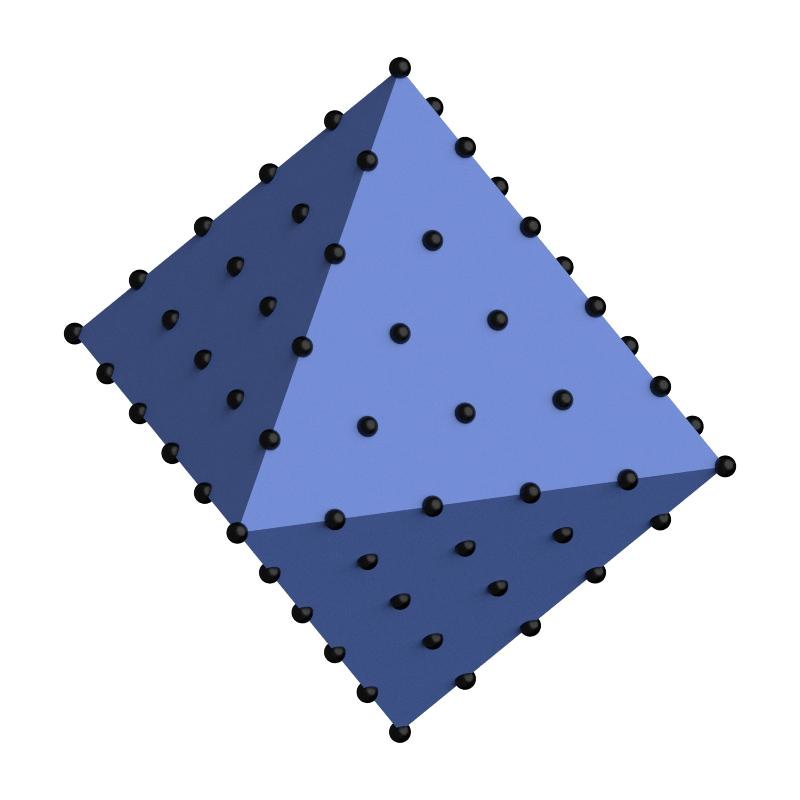
$\quad\longrightarrow\quad$

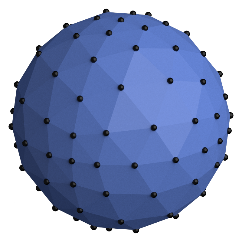
Figure 1: Construction of the linear lattice on $S_{2}$ for $m=3$. First we fill the faces of the octahedron, and then project them out onto the sphere. It can be seen that the points are more densely distributed around the corners of the original octahedron, and more spread out in the middle of the faces.

We begin with the linear partitioning $L_{m}(k)$ on the sphere $S_{k}$ in $k+1$ dimensions, given by

$$L_{m}(k) \coloneqq\left\{\frac{1}{M}\left(s_{0}j_{0},\dots,s_{k}j_{k}\right)\middle|\,\sum_{i=0}^{k}j_{i}=m,\;\forall i\in\{0,\dots,k\}:\,s_{i}\in\{\pm 1\},\,j_{i}\in\mathbb{N}\right\}\,,$$ (2)

with

$$\qquad M\coloneqq\sqrt{\sum_{i=0}^{k}j_{i}^{2}}\,.$$ (3)

As depicted in fig. 1, it can be visualized as distributing points evenly on higher dimensional versions of the octahedron, and then projecting them onto the sphere. Note that some testing on this partitioning has already been carried out in [4].

One apparent problem with this approach is that group elements are distributed more densely around the vertices of the octahedron, and more sparsely in the middle of the faces. As one might expect, this will cause systematic deviations from the full gauge group, if not corrected for.

To counteract such effects, we assign a probabilistic weight attributed to each point. This weight $w$ is defined as the volume of the Voronoi cell [5, 6] of the point using the canonical metric on $S_{k}$ derived from the Euclidean distance. For the linear partitionings this can be approximated with

$$w\approx\left(\frac{\sqrt{2}}{M}\right)^{k}.$$ (4)

Further details of this calculation can again be found in [1].

2.1.1 Volleyball Partitionings

Similarly to the linear lattices, we can also construct a partitioning by distributing points on the faces of a hypercube. On $S_{2}$ the result looks somewhat reminiscent of a Volleyball, which is why we will refer to this approach as the volleyball partitioning:

$$\begin{split}V_{m}(k)&\coloneqq\left\{\frac{1}{M}\left(s_{0}j_{0},\dots,s_{k}j_{k}\right)\middle|\,(j_{0},\dots,j_{k})\in\left\{\text{all perm. of }(m,a_{1},\dots,a_{k})\right\},\right.\\ &\hskip 227.62204pt\left.\,s_{i}\in\{\pm 1\},\,a_{i}\in\{0,\dots,m\}\vphantom{\frac{1}{M}}\right\}\end{split}$$ (5)

where $M$ again defined in eq. 3. Furthermore, we can also include the trivial case of not subdividing the faces of the hypercube at all:

$$V_{0}(k) \coloneqq\left\{\frac{1}{\sqrt{k+1}}\left(s_{0},\dots,s_{k}\right)|\,s_{i}\in\{\pm 1\}\right\}\,.$$ (6)

Similarly to the linear partitionings, points are again distributed more densely towards the corners of the hypercube. In fact, the weights turn out to be quite similar and are given by

$$w\approx\left(\frac{1}{M}\right)^{k}.$$ (7)

For details, we again refer to [1].

2.1.2 Fibonacci Partitionings

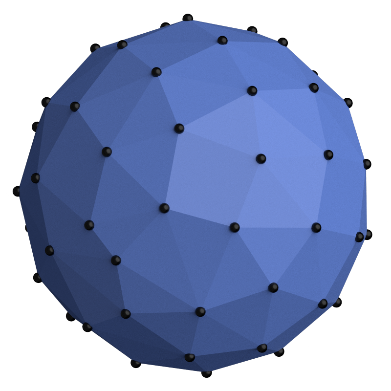
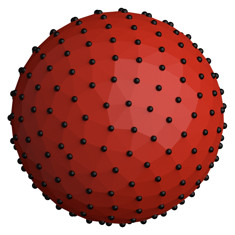
Figure 2: Fibonacci lattices with $64$ lattice points on the left, and $256$ lattice points on the right. It can be seen that the points are spread evenly over the whole sphere, but lack any local geometric structure.

The final partitioning of SU$(2)$ considered in this work is a generalized version of the so-called Fibonacci lattice. For a given size $n$, it is usually constructed within a unit square $[0,1)^{2}$ as

$$\Lambda_{n}^{2}=\left\{\tilde{t}_{m}\middle|0\leq m<n,\,\,m\in\mathbb{N}\right\}\qquad\text{with}\qquad\tilde{t}_{m} =\begin{pmatrix}x_{m}\\ y_{m}\end{pmatrix}=\left(\frac{m}{\tau}\quad\mathrm{mod}\quad 1,\frac{m}{n}\right)^{t}\,,$$ (8)

$$\text{and}\,\,\,\qquad\tau =\frac{1+\sqrt{5}}{2}\,.$$ (9)

Typically it is then mapped onto other surfaces, such as spheres or circles. Some examples for $S_{2}$ can be seen in fig. 2. One of the main advantages of this approach, is that we have precise control over the number of elements in our partition. This contrary to the case of linear and volleyball partitionings where the lattice size scales roughly as $n\sim m^{3}$, and leaves gaps in between the available sizes. Furthermore, the distribution of points is uniform for larger lattices. Thus no weighting of the lattice points is needed, and we can set $w=1$. When taking a closer look at fig. 2, we can however see that the local structure of this partitioning is fairly irregular. As seen later, this will cause systematic deviations for smaller values of $\beta$.

To construct a Fibonacci partitioning on a $k$-dimensional manifold, we begin by generalizing eq. 8 to the hypercube $[0,1)^{k}$ embedded in $\mathbb{R}^{k}$:

$$\Lambda_{n}^{k} =\left\{t_{m}\middle|0\leq m<n,\,\,m\in\mathbb{N}\right\}$$

$$t_{m} =\begin{pmatrix}t_{m}^{1}\\ t_{m}^{2}\\ \vdots\\ t_{m}^{k}\end{pmatrix}=\begin{pmatrix}\frac{m}{n}&\\ a_{1}\,m\quad&\mathrm{mod}\quad 1\\ \vdots&\\ a_{k-1}\,m\quad&\mathrm{mod}\quad 1\\ \end{pmatrix}$$

with

$$\frac{a_{i}}{a_{j}}\notin\mathbb{Q}\quad\textrm{for}\quad i\neq j\textrm{,}$$

where $\mathbb{Q}$ denotes the field of rational numbers. The square roots of the prime numbers provide a simple choice for the constants $a_{i}$:

$$(a_{1},a_{2},a_{3},\dots)=(\sqrt{2},\sqrt{3},\sqrt{5},\dots)$$

Then a volume preserving map to the manifold needs to be constructed. This can be done by studying the jacobian obtained by introducing spherical coordinates on $S_{3}$ [1]. The result is given by

$$F_{n} =\left\{z\left(\psi_{m}(t_{m}^{1}),\theta_{m}(t_{m}^{2}),\phi_{m}(t_{m}^{3})\right)\middle|\,0\leq m<n,\,\,m\in\mathbb{N}\right\}\,,$$

with spherical coordinates on $S_{3}$

$$z(\psi,\theta,\phi)=\left(\begin{array}[]{l}\cos\psi\\ \sin\psi\cos\theta\\ \sin\psi\sin\theta\cos\phi\\ \sin\psi\sin\theta\sin\phi\end{array}\right)$$ (10)

and

$$\begin{split}\psi_{m}(t_{m}^{1})&=\Phi_{1}\left(t_{m}^{1}\right)=\Phi_{1}\left(\frac{m}{n}\right)\,,\\ \theta_{m}(t_{m}^{2})&=\Phi_{2}\left(t_{m}^{2}\right)=\cos^{-1}\left(1-2(m\sqrt{2}\mod 1)\right)\,,\\ \phi_{m}(t_{m}^{3})&=\Phi_{3}(t^{3}_{m})=2\pi(m\sqrt{3}\mod 1)\,.\end{split}$$

3 Methods

With the construction done, it is now time to investigate the behavior of the proposed partitionings. For this, we work on a hyper-cubic, Euclidean lattice with the set of lattice sites

$$\Lambda\ =\ \{n=(n_{0},\ldots,n_{d-1})\in\mathbb{N}_{0}^{d}:n_{\mu}=0,1,\ldots,L-1\}\,,$$

with $L\in\mathbb{N}$. At every site there are $d\geq 2$ link variables $U_{\mu}(n)\in\mathrm{SU}(2)$ connecting to sites in forward direction $\mu=0,\ldots,d-1$. We define the plaquette operator as

$$P_{\mu\nu}(n)\ =\ U^{~{}}_{\mu}(n)U^{~{}}_{\nu}(n+\hat{\mu})U^{\dagger}_{\mu}(n+\hat{\nu})U^{\dagger}_{\nu}(n)\,,$$ (11)

where $\hat{\mu}\in\mathbb{N}_{0}^{d}$ is the unit vector in direction $\mu$. In terms of $P_{\mu\nu}$ we can define Wilson’s lattice action [7]

$$S=-\frac{\beta}{2}\sum_{n}\sum_{\mu<\nu}\mathrm{Re}\,\mathrm{Tr}\,P_{\mu\nu}(n)\,,$$ (12)

with $\beta$ the inverse squared gauge coupling. We will use the Metropolis Markov Chain Monte Carlo algorithm to generate chains of sets $\mathcal{U}_{i}$ of link variables $\mathcal{U}=\{U_{\mu}(n):n\in\Lambda,\mu=0,\ldots,d-1\}$ distributed according to

$$\mathbb{P}(\mathcal{U})\ \propto\ \exp[-S(\mathcal{U})]\,.$$ (13)

This is implemented by iterating over all lattice sites $n$ and all directions $\mu$. For each pair, we then

1. generate a proposal $U_{\mu}^{\prime}(n)$ from $U_{\mu}(n)$.

2. compute $\Delta S=S(U_{\mu}^{\prime}(n))-S(U_{\mu}(n))$.

3. accept with probability

   $$\mathbb{P}_{\mathrm{acc}}=\min\left\{1,\ \exp(-\Delta S)\frac{w(U_{\mu}^{\prime}(n))}{w(U_{\mu}(n))}\right\}\,.$$ (14)

This procedure is repeated $N_{\mathrm{hit}}=10$ times per $n$ and $\mu$ before moving on to the next pair $(n,\mu)$.

For the partitionings of SU$(2)$ the proposal $U_{\mu}^{\prime}(n)$ is randomly picked from the neighbors of $U_{\mu}(n)$. In the case of the linear and volleyball partitionings we will test both the calculated, and trivial ($w=1$) probabilistic weights. As the distribution of points in the Fibonacci lattices is approximately uniform, only trivial weights are used here.

The full gauge group is approximated by four double precision floating point numbers, storing $x_{i}$ from eq. 1. To stay in SU$(2)$ we furthermore, restrict $\sum_{i}x_{i}^{2}=1$. New proposals $U_{\mu}^{\prime}(n)$ are generated by multiplying with a random element $V\in\mathrm{SU}(2)$ which has a maximum distance $\delta$ to the identity element $1\in\mathrm{SU}(2)$. $\delta$ controls the average magnitude of $\Delta S$ in step 2 of the algorithm and is tuned towards an acceptance rate of about $50\%$ in step 3. As we can pick $\delta$ arbitrarily small (within the limits of floating point precision), we can avoid the aforementioned freezing transition. The results obtained with this quasi continuous representation of SU$(2)$ will be referred to as reference results in the following.

The main observable we will study in this proceeding is the plaquette expectation value defined as

$$\langle P\rangle=\frac{1}{N}\sum_{i=1}^{N}\ P(\mathcal{U}_{i})$$ (15)

with

$$P(\mathcal{U})=\frac{2}{d(d-1)L^{d}}\sum_{n}\sum_{\mu<\nu}\mathrm{Re}\,\mathrm{Tr}\,P_{\mu\nu}(n)\,.$$

All results presented here, were obtained in $3+1$ dimensions, with $L^{4}=8^{4}$ lattice volume. The starting configuration was chosen to be either uniform (cold), or fully random (hot). Statistical errors for $P$ are computed based on the so-called $\Gamma$-method detailed in Ref. [8] and implemented in the publicly available software package hadron [9].

4 Results

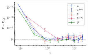
(a) $\beta=1.0$

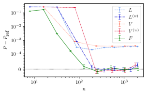
(b) $\beta=3.0$

Figure 3: Difference between partitioning and reference plaquette expectation value, as a function of the partitioning size $n$. Linear and volleyball partitionings are shown with and without weighting. The partitioning data was averaged over $10^{5}$, and the reference data over $10^{6}$ sweeps of the lattice.

First we want to investigate, how well our partitionings reproduce the reference data, when not affected by the freezing transition. For this $3000$ thermalization sweeps, followed by $10^{5}$ measurement sweeps were performed once for $\beta=1.0$ and then again for $\beta=3.0$. This data was then compared to reference data obtained over $10^{6}$ measurement sweeps. The results can be found in fig. 3. For $\beta=1.0$ both unweighted and weighted linear and volleyball partitionings mostly reproduce the reference case. Noteworthy exceptions are $L_{1}$ and $V_{0}$, which are already past their freezing transition, as well as $V_{1}$ and $L_{2}$ which are pretty close to theirs. For the Fibonacci partitionings no significant deviation is observed for sizes $n\geq 64$. For $\beta=1$ $F_{8}$ is again past its freezing transition. For $F_{16}$ and $F_{32}$ the transition is only expected for significantly bigger values of $\beta$. A likely explanation for the deviation is thus the irregular structure of the partitioning.

At $\beta=3.0$ the picture changes. We now see a clear necessity for considering the Voronoi weights for the linear and volleyball lattices. Without these weights, we see a persistent significant deviation from the reference data. It is worth noting, that this deviation seems to be mostly independent of the partitioning size. This confirms that it is indeed caused by the uneven density of elements in the partition.

The results for the Fibonacci lattices look similar to the ones at $\beta=1.0$, but shifted to the right. Agreement with the reference data is now achieved for $n\geq 128$. The deviations of the smaller partitionings are most likely to blame on their now much closer freezing transitions.

4.1 Freezing Transition

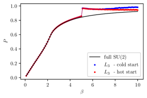
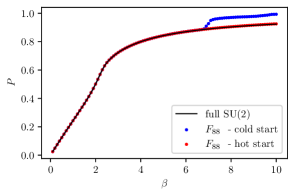
Figure 4: Hysteresis loops for the Fibonacci partitioning $F_{88}$ and the linear partitioning with weights included $L_{3}$. Both have $n=88$ elements.

To study this freezing transition in more detail, we look at $\beta\in\{0.1,0.2,\dots,9.9,10.0\}$. For each value of $\beta$, $7000$ sweeps are performed, once with a hot, and once with a cold starting configuration. The plaquette is then measured by averaging over the last $3000$ iterations.

Such scans in $\beta$ can be found in fig. 4. $\beta_{c}$ is then estimated to be the last value before a significant jump in $\langle P\rangle$, or a significant disagreement between the hot and cold start. We have checked that the such determined critical $\beta$-values do not depend significantly on the volume.

In fig. 5 we show the $\beta_{c}$-values at which the freezing transitions takes place as a function of the number $n$ of elements in the set of points or the subgroups. It can be seen that the Fibonacci lattices outperform all other partitionings, and thus offer the biggest range of beta for a given size $n$. Furthermore, it seems that $\beta_{c}$ is smaller when considering the Voronoi weights for the linear and volleyball lattices, compared to the trivial weights.

In Ref. [3] the authors find that the critical $\beta$-value can be computed theoretically, at least approximately, for the finite subgroups:

$$\beta_{c}(N)\approx\frac{\ln\left(1+\sqrt{2}\right)}{1-\cos(2\pi/N)}\,.$$ (16)

Here $N$ denotes the power to which the closest neighbors $g$ of the identity need to be taken, such that $g^{N}=1$. Fibonacci, linear and volleyball partitionings however lack group structure. Therefore, it is not guaranteed that there is an $N\in\mathbb{N}$ for which $g^{N}=1$.

Thus, we have to approximate the order $N$. For (approximately) isotropic discretisations such as the finite subgroups and the Fibonacci partitioning a global average over the point density is bound to yield a good approximation for the elements in $C(G)$ and therefore $N$. The volume of the three-dimensional unit sphere is $2\pi^{2}$. If we then assume a locally primitive cubic lattice, the average distance of $n$ points in $S_{3}$ becomes

$$d(n)=\left(\frac{2\pi^{2}}{n}\right)^{1/3}\,.$$ (17)

Two points of this distance together with the origin form a triangle with the opening angle

$$\alpha(n)=2\arcsin\left(\frac{d(n)}{2}\right)\,,$$ (18)

thus, a first approximation of the cyclic order is obtained by

$$\tilde{N}(n)=\frac{2\pi}{\alpha(n)}\,,$$ (19)

which solely depends on the number $n$ of elements in the partition.

Note that the assumption of a primitive cubic lattice is even asymptotically incorrect for all the partitionings discussed in this work, and at best a good approximation. How good an approximation it is, can only be checked numerically. In specific cases, it needs further refinement.

In particular, in the case of the Fibonacci partitioning the approximation has to be adjusted. Since the points are distributed irregularly in this case, a path going around the sphere does not lie in a two-dimensional plane. Instead, it follows some zigzag route which is longer than the straight path. Assuming the optimal maximally dense packing, we expect the points to lie at the vertices of tetrahedra locally tiling the sphere. The length of the straight path would then correspond to the height of the tetrahedron, whereas the length of the actual path corresponds to the edge length. Their ratio is $\sqrt{3/2}$, so $\tilde{N}$ has to be rescaled by this factor to best describe $\beta_{c}$ for the Fibonacci partitioning.

We show the curve eq. 16 using $\tilde{N}(n)$ and $\sqrt{3/2}\tilde{N}$, respectively, in addition to the data in fig. 5. The version with $\tilde{N}$ is in very good agreement with the results obtained for the finite subgroups, while the rescaled version matches the values for the Fibonacci partitioning remarkably well.

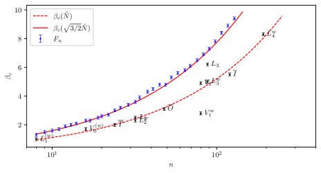
Figure 5: The critical value $\beta_{c}$ as a function of the number $n$ of elements in the set. The lines represent the approximation eq. 16 where the order $\tilde{N}(n)$ is obtained from eq. 19.

5 Conclusion

In this proceeding, we have presented several asymptotically dense partitionings of SU$(2)$, which do not represent subgroups of SU$(2)$ but which have adjustable numbers of elements. MC simulations restricted to these partitionings turned out to give good agreement with the standard simulation code, in particular when correcting for anisotropies in the point distribution.

In addition we have investigated the so-called freezing transition for the partitions and for all finite subgroups of SU$(2)$. The main result visualised in fig. 5 is that the partitioning $F_{k}$ based on Fibonacci lattices allows for a flexible choice of the number of elements by adjusting $k$ and at the same time larger $\beta_{c}$-values compared to finite subgroups and the other discussed partitionings. Thus, Fibonacci based discretisations provide the largest simulatable $\beta$-range at fixed $n$.

Coming back to the introduction, using the partitionings proposed here does not pose any problem even at very large $\beta$-values at least in Monte Carlo simulations. This leaves us optimistic for their applicability in the Hamiltonian formalism for tensor network or quantum computing applications.

References

- [1] T. Hartung, T. Jakobs, K. Jansen, J. Ostmeyer and C. Urbach, The European Physical Journal C 82, 237 (2022), https://doi.org/10.1140/epjc/s10052-022-10192-5.
- [2] J. L. Britton, The Mathematical Gazette 42, 139–140 (1958).
- [3] D. Petcher and D. H. Weingarten, Phys. Rev. D 22, 2465 (1980).
- [4] D. C. Hackett et al., Phys. Rev. A 99, 062341 (2019), arXiv:1811.03629 [quant-ph].
- [5] G. Voronoi, Journal für die reine und angewandte Mathematik (Crelles Journal) 1908, 97 (1908), https://doi.org/10.1515/crll.1908.133.97.
- [6] G. Voronoi, Journal für die reine und angewandte Mathematik (Crelles Journal) 1908, 198 (1908), https://doi.org/10.1515/crll.1908.134.198.
- [7] K. G. Wilson, Phys. Rev. D 10, 2445 (1974).
- [8] ALPHA Collaboration, U. Wolff, Comput. Phys. Commun. 156, 143 (2004), arXiv:hep-lat/0306017, [Erratum: Comput.Phys.Commun. 176, 383 (2007)].
- [9] B. Kostrzewa et al., hadron: package to extract hadronic quantities, https://github.com/HISKP-LQCD/hadron, 2020, R package version 3.1.0.
- [10] R Core Team, R: A Language and Environment for Statistical Computing, R Foundation for Statistical Computing, Vienna, Austria, 2019.