Abstract

As an alternative gravity model we consider an extended Einstein-Maxwell gravity containing a gauge invariance property. Extension is assumed to be addition of a directional coupling between spatial electromagnetic fields with the Ricci tensor. We will see importance of the additional term in making a compact stellar object and value of its radius. As an application of this model we substitute ansatz of magnetic field of a hypothetical magnetic monopole which has just time independent radial component and for matter part we assume a perfect fluid stress tensor. To obtain spherically symmetric internal metric of the perfect fluid stellar compact object we solve Tolman-Oppenheimer-Volkoff equation with a polytropic form of equation of state as $p(\rho)=a\rho^{2}$. Using dynamical system approach we study stability of the solutions for which arrow diagrams show saddle (quasi stable) for $a<0$ (dark stars) and sink (stable) for $a>0$ (normal visible stars). We check also the energy conditions, speed of sound and Harrison-Zeldovich-Novikov static stability criterion for obtained solution and confirm that they make stable state.

1 Introduction

High energy astronomical compact objects in cosmic scales are considered as excellent laboratories for investigating astrophysical phenomena, and their relationship with nuclear and elementary particles physics has opened a new approach to modern astrophysics. High energy astronomical compact objects include for instance, neutron stars, quark stars, boson stars, white dwarfs, and black holes can be formed when a massive star runs out of its fuel and therefore cannot remain stable against its own gravity and then collapses [1],[2]. Depending on total value of the mass of the star, the collapse changes the star‘s configuration and then initiates a new structure. In general a star is stable when the pressure force from the gas atoms is equal to its gravitational force and otherwise will be unstable. The stability of the star can be investigated in the presence of both electric and magnetic fields. Solving the Einstein-Maxwell field equations for compact stars with the charged anisotropic fluid model give more stable solutions than for neutral stars. The presence of charges create repulsive forces against the gravitational force, and so it causes to stable more for stars with higher total mass and so larger redshift [3]. In the core of neutron stars, there is possibility of hadron-quark phase transition. Charged quarks can create more stable quark stars than neutron nuclei. In theories beyond the standard model, the effect of dark matter on the internal structure of the neutron stars suggests that the neutron stars is mixed with dark matter in the core and it is surrounded by a shell. This feature affects the stellar mass-radius relation such that dark matter effects are responsible for reducing the stellar mass, while the main effect of the shell is to increase the stellar radius [4]. In compact objects mixed with normal matter and dark matter, as the central pressure of dark matter increases, the neutron stars becomes unstable and the white dwarfs will have unusual masses and radii. Therefore, the resulting object will have unusually small mass and radius [5]. When enough non-destructive dark matter accumulates on a neutron stars, it creates a central degenerate star. If the mass of the dark matter in the star reaches the Chandrasekhar mass limitation of the star, the dark matter leads to collapse the mixed neutron stars [6]. The stability can also be investigated for compact stars that are affected by strong magnetic fields and so affect the process of stellar evolution. Surface Magnetic fields observed in stars can be divided into two categories: the fossil and dynamo hypothesis. The fossil hypothesis is used to explain magnetism in massive stars, and the dynamo hypothesis, which is used for the inner space of stars, shows the effects of a strong magnetic field on the propagation of gravitational waves [7]. Stability of stars has provided via many gravitational models in which the main question is whether a small perturbation can rapidly decay in comparison to the model’s parameters or not [8]. Hydrodynamical simulations in general theory of relativity have been applied to investigate the dynamical stability of differentially rotating neutron stars [9]. Dynamical instability of a star undergoing a dissipative collapse, has been explored by considering the role of pressure anisotropy [10]. In general it is confirmed that the magnetic fields has a main role in evolution and stability of the stars. For instance it is obvious that sunspots are the largest concentration of complex magnetic flux [11]. Also there is inferred that energy source of emission from magnetars is magnetic field (see for instance [12] and [13]). Furthermore, the origin and dynamics of magnetic fields in the surface of massive stars have been studied in ref [14]. Extensive study of the evolution of magnetic field has been performed in rotating radiative zones of intermediate-mass stars [15]. Due to the importance of the magnetic field effects on stability of stars we like to study stability of a spherical perfect fluid stellar compact object in presence of radial magnetic field of hypothetical magnetic monopoles [16], [17],[18],[19],[20],[21]. Pierre Curie pointed out in 1894 [22] that magnetic monopoles could conceivably exist, despite not having been seen so far. From quantum theory of matter, Paul Dirac [23] showed that if any magnetic monopoles exist in the universe, then all electric charge in the universe must be quantized (Dirac quantization condition)[24]. Since Dirac’s paper, several systematic monopole searches have been performed. Experiments in 1975 [25] and 1982 [26] produced candidate events that were initially interpreted [25] as monopoles, but are now regarded inconclusive. Therefore, it remains an open question whether the magnetic monopoles exist. Further advances in theoretical particle physics, particularly developments in grand unified theories and quantum gravity, have led to more compelling arguments that monopoles do exist. Joseph Polchinski, provided an argument from string theory, confirming the existence of magnetic unipolarity, which has not yet been observed by experimental physics [27]. These theories are not necessarily inconsistent with the experimental evidence. In some theoretical models, magnetic monopoles are unlikely to be observed, because they are too massive to create in particle accelerators, and also too rare in the Universe to enter a particle detector with much probability [27].
It is well known that the ordinary matter consists of fermions in fact. But the fermions composed in such a way that the final products have integer spins. For real fermions as matter sources, we have to use spinors which can not be directly included in Einstein’s GR equation. By the way, in cosmology, we consider the perfect fluid as a thermodynamics representation of the matter content of the universe and it is not constructed from some elementary particles. The energy density and pressure are two independent thermodynamics variables and they are related to each other via equation of state $p(\rho).$ However there is ‘Thomas-Fermi approximation‘ where two assumptions are considered usually: (a) All gravitational and other possible sources are slowly varying fields with respect to fermion fields and so they do not interact with each other so that one can use mean field theory (macroscopic quantities) instead of dynamical microscopic fermion fields. (b) the fermion gas is at equilibrium so that all the macroscopic quantities are time independent and its stress tensor behaves as perfect fluid which in the isotropic form is described by mass/energy density $\rho$ and hydrostatic isotropic pressure $p$ (see for instance [28] and [29] for more details). On the other side exotic $\alpha$ dependent term in our used lagrangian (see eq. (2.1)) produces $\Theta$ term of stress tensor (3.9) which does not satisfies covariant conservation condition (Bianchi identity) alone and thus we need other matter stress tensor to balance this inconsistency. Hence we assume the matter term to be a perfect fluid stress tensor with polytropic type of equation of state $p=a\rho^{b}.$ Usually the latter form of equation of state is used for neutron stars with $b=2$. By using dynamical system approach (see introduction section in [36]) and solving TOV equations we obtained parametric critical points in the phase space and to check which of the internal metric solutions near the critical points in phase space are physical we investigate null energy condition (NEC), weak energy condition (WEC) and strong energy condition (SEC) together with regularity, causality and Harrison-Zeldovich-Novikov static stability (HZN) conditions. Layout of this paper is as follows.
In section two we present proposed modified Einstein-Maxwell gravity model together with its physical importance. As an magnetic source to produce a spherically symmetric static metric of an stellar object we consider radial magnetic field of a magnetic monopole charge and derive TOV equations of internal metric of the system for stress tensor of perfect isotropic fluid. We see that the equations of the fields are nonlinear and so we must be use dynamical system approach to obtain solutions of the fields near the critical points in phase space. This is done in the section of third. Physical analysis of the obtained solutions are dedicated to the section four.The last part of this work is devoted to conclusions and prospects for the development of the work.

2 Gravity model

Let us start with the following generalized Einstein Maxwell gravity.

$$I=\int d^{4}x\sqrt{g}\left[\frac{R}{16\pi}+\frac{1}{4}F_{\mu\nu}F^{\mu\nu}+\alpha F_{\rho\mu}R^{\mu}_{\eta}F^{\eta\rho}\right]+I_{matter},$$ (2.1)

where $g$ is absolute value of determinant of the metric field and dimensions in the coupling constant $\alpha$ is square of length and we write the action in the geometric units $c=G=1$. $R_{\mu\nu}(R)$ is Ricci tensor (scalar) and anti-symmetric electromagnetic tensor field $F_{\mu\nu}$ is defined by $F_{\mu\nu}=\nabla_{\mu}A_{\nu}-\nabla_{\nu}A_{\mu}$ which for torsion free Riemannian geometries can be rewritten as that

$$F_{\mu\nu}=\partial_{\mu}A_{\nu}-\partial_{\nu}A_{\mu}.$$ (2.2)

In fact motivation of such a model is given previously in the paper [31] to investigate how is broken conformal invariance symmetry of the electromagnetic field in the cosmological context. This is needed to produce large scale magnetic fields $(\sim Mpc)$ with high intensity. Regretfully, a pure $U(1)$ gauge theory with the standard Lagrangian $F_{\mu\nu}F^{\mu\nu}/4$ is conformal invariant and so for a Robertson-Walker spacetime with scale factor $a(t),$ the magnetic field intensity decreases as $1/a^{2}$ and in the de Sitter inflationary epoch is ineffective and the vacuum energy density is dominated. While, today, it is obvious that magnetic fields are present throughout the universe and it plays an important role in astrophysical situations. For instance presence of high intensity magnetic field generates a high pressure which prevents the star from contracting. Even it is necessary to initiate substantial currents in superconducting cosmic strings which can be possible just by presence of high intensity cosmic magnetic fields (see [31] and reference therein).To do so we must add some additional suitable scalars to the Lagrangian $F_{\mu\nu}F^{\mu\nu}/4$ such as given in the equation (2.1). It is easy to check that the above action functional is not changed by transforming $A_{\mu}\to A_{\mu}+\partial_{\mu}\xi$ where $A_{\mu}$ is four vector electromagnetic potential field and $\xi$ is a scalar gauge field, because by using the mentioned transformation, we obtain $F_{\mu\nu}\to F_{\mu\nu}$. Varying the above action with respect to the metric tensor field $g_{\mu\nu}$ reads the Einstein metric field equations such that

$$G_{\mu\nu}=8\pi T_{\mu\nu}^{total}=8\pi[T_{\mu\nu}^{EM}+\alpha\Theta_{\mu\nu}+T_{\mu\nu}^{(matter)}],$$ (2.3)

where

$$G_{\mu\nu}=R_{\mu\nu}-\frac{1}{2}g_{\mu\nu}R,$$ (2.4)

is the Einstein tensor defined by the Ricci tensor $R_{\mu\nu}$ and the Ricci scalar $R=g^{\mu\nu}R_{\mu\nu}$,

$$T^{EM}_{\mu\nu}=-\frac{1}{8}\left[F_{\mu\alpha}F^{\alpha}_{\nu}+F_{\beta\nu}F^{\beta}_{\mu}-\frac{1}{2}g_{\mu\nu}F_{\alpha\beta}F^{\alpha\beta}\right]$$ (2.5)

is traceless electromagnetic field stress tensor,

$$\Theta_{\mu\nu}=\frac{1}{4}g_{\mu\nu}F_{\rho\alpha}R^{\alpha}_{\eta}F^{\eta\rho}-\frac{1}{2}[F_{\rho\mu}R_{\nu\eta}F^{\eta\rho}+F_{\rho\eta}R^{\eta}_{\mu}F^{\rho}_{\nu}+F_{\rho\mu}R^{\rho}_{\eta}F^{\eta}_{\nu}]$$

$$+\frac{1}{4\sqrt{g}}\partial_{\alpha}\left[\partial_{\eta}\left(\sqrt{g}F^{\alpha}_{\rho}F^{\eta\rho}\right)\right]g_{\mu\nu}-\frac{1}{2\sqrt{g}}\partial_{\mu}\left(\sqrt{g}F^{\alpha}_{\rho}F^{\eta\rho}\right)\Gamma_{\nu\alpha\eta}$$

$$-\frac{1}{8\sqrt{g}}g_{\eta\mu}g_{\sigma\nu}\partial_{\lambda}\left[\partial_{\alpha}\left(\sqrt{g}F^{\lambda}_{\rho}F^{\eta\rho}\right)g^{\alpha\sigma}\right]$$

$$-\frac{1}{8\sqrt{g}}g_{\sigma\mu}g_{\lambda\nu}\partial_{\eta}\left[\partial_{\alpha}\left(\sqrt{g}F^{\lambda}_{\rho}F^{\eta\rho}\right)g^{\alpha\sigma}\right]+\frac{1}{8\sqrt{g}}g_{\lambda\mu}g_{\eta\nu}\partial_{\sigma}\left[\partial_{\alpha}\left(\sqrt{g}F^{\lambda}_{\rho}F^{\eta\rho}\right)g^{\alpha\sigma}\right]$$ (2.6)

is gravity-photon interaction stress tensor and $T_{\mu\nu}^{(matter)}$ is matter part stress tensor respectively. Here we choose matter content of the system to be isotropic perfect fluid with stress tensor [32]

$$(T^{matter})^{\mu}_{\nu}=diag(-\rho,p,p,p)$$ (2.7)

where pressure is related to the density via a suitable equation of state $p(\rho)=a\rho^{b}.$ Electromagnetic Maxwell field equation is given by varying the action functional (2.1) with respect to the gauge field $A_{\mu}$ such that

$$\nabla_{\nu}F^{\mu\nu}=2\alpha J^{\mu},$$ (2.8)

where the four current density, $J^{\mu}$, is defined by

$$J^{\mu}=\nabla_{\lambda}C^{\lambda\mu}$$ (2.9)

in which $C^{\lambda\mu}$ is anti-symmetric tensor

$$C^{\lambda\mu}=-C^{\mu\lambda}=\left(R^{\mu}_{\eta}F^{\eta\lambda}-R^{\lambda}_{\eta}F^{\eta\mu}\right).$$ (2.10)

One can show that the Maxwell equation (2.8) can be rewritten as follows.

$$\nabla_{\nu}\tilde{F}^{\mu\nu}=0,~{}~{}~{}\tilde{F}^{\mu\nu}=F^{\mu\nu}+2\alpha C^{\mu\nu}$$ (2.11)

and for arbitrary anti-symmetric tensor $O^{\mu\nu}$ we have

$$\nabla_{\mu}O^{\mu\nu}=\frac{\partial_{\nu}(\sqrt{g}O^{\mu\nu})}{\sqrt{g}}$$ (2.12)

in torsion free curved spacetimes. In the differential geometry formalism of the electromagnetic field, the above antisymmetric Faraday tensor can be written as follows [33].

$$\textbf{F}=\frac{1}{2}F_{\mu\nu}dx^{\mu}\wedge dx^{\nu}=\textbf{B}+\textbf{E}\wedge dx^{0}=d\textbf{A}+\textbf{E}\wedge dx^{0}$$ (2.13)

in which

$$\textbf{E}=E_{i}dx^{i}$$ (2.14)

is 1-form electric field and

$$\textbf{B}=\frac{1}{2}\epsilon_{ijk}B^{i}dx^{j}\wedge dx^{k}$$ (2.15)

is 2-form magnetic field. In fact they are spatial vector fields and $i,j=1,2,3$ correspond to spatial coordinates while $x^{0}$ denotes to time coordinate in the curved background spacetime. In the above equation $\epsilon_{ijk}$ is third rank totally antisymmetric Levi Civita tensor density. Its numeric value is $+1(-1)$ for $\{i,j,k\}=\{1,2,3\}$ and for any even (odd) permutations while it takes zero value for any two repeated indices. The equation (2.13) can be rewritten to the following form also [10].

$$F_{\mu\nu}=n_{\mu}E_{\nu}-n_{\nu}E_{\mu}+\epsilon_{\mu\nu\eta\lambda}B^{\eta}n^{\lambda}$$ (2.16)

where $n_{\mu}$ is a unit time-like vector field and is normal to the spatial 3D hypersurface $x^{0}=const$ and so can be defined by $n^{\mu}=-\nabla_{\mu}x^{0}/||\nabla_{\mu}x^{0}||.$ Consequently the electric and magnetic fields components $\{E_{i},B_{i}\}$ are measured by a normal observer aligned to $n_{\mu}$ and so they are absolutely spatial vector fields $E_{\mu}n^{\mu}=0=B_{\mu}n^{\mu}.$ From ADM formalism in the $1+3$ decomposition of any 4D curved background spacetime metric the whole of spacetime can be foliated into hypersurfaces with constant time coordinate $x_{0}$ where $h_{ij}=g_{ij}$ are spatial 3-metric defined on the spacelike hypersurfaces. In the other words the general form of line element $ds^{2}=g_{\mu\nu}dx^{\mu}dx^{\nu}$ reads

$$ds^{2}=-\alpha^{2}dt^{2}+h_{ij}(dx^{i}+\beta^{i}dt)(dx^{j}+\beta^{j}dt)$$ (2.17)

in which $\alpha$ is lapse function and $\beta^{i}$ is shift vector. In the definition (2.16) $\epsilon_{\mu\nu\eta\lambda}$ is fourth rank totally antisymmetric Levi Civita tensor density. Its numeric value is $+1(-1)$ for $\{\mu,\nu,\eta,\lambda\}=\{0,1,2,3\}$ and for any even (odd) permutations while it takes zero value for any two repeated indices. For time independent static curved spacetimes the line element (2.17) takes a simpler forme because $\beta^{i}=0$ and $\alpha$ and $h_{ij}$ take on just spatial coordinates $x^{i}$. In this case we can apply a suitable coordinates transformation to remove all non-diagonal components of $h_{ij}$ such that

$$ds^{2}=-(\alpha dt)^{2}+(\gamma_{i}dq^{i})^{2}$$ (2.18)

in which $d\ell_{i}=\gamma_{i}dq_{i}$ has length dimension and $dq^{i}$ is spatial coordinates used in a local curvilinear frame in the 3D space [34]. For the line element (2.18) the identity (2.13) reads

$$F_{it}=\sqrt{\alpha}\gamma_{i}E_{i},~{}~{}~{}F_{jk}=\epsilon_{ijk}B_{i}\gamma_{j}\gamma_{k}$$ (2.19)

in which repeated indexes for $\epsilon_{ijk}$ do not follow the Einstein summation rule and just follows permutation cycles. In the next section we write the Einstein equations and the Tolman-Oppenheimer-Volkoff equation for internal metric of a spherically symmetric static compact stellar object in presence of magnetic field of a magnetic monopole charge and stress tensor of a perfect fluid with density $\rho$ and pressure $p$ with polytropic form of equation of state $p=a\rho^{2}.$ This form of equation of state is used usually for Neutron stars [35].

3 Tolman-Oppenheimer-Volkoff equation

Line element for a general spherically symmetric curved spacetime is given by

$$ds^{2}=-X(t,r)dt^{2}+Y(t,r)dr^{2}+r^{2}(d\theta^{2}+\sin^{2}\theta d\varphi^{2})$$ (3.1)

for which the equations (2.19) reads

$$F_{\mu\nu}=\left(\begin{array}[]{cccc}0&-\sqrt{XY}E_{r}&-\sqrt{X}rE_{\theta}&-\sqrt{X}r\sin\theta E_{\varphi}\\ \sqrt{XY}E_{r}&0&\sqrt{Y}rB_{\varphi}&-\sqrt{Y}r\sin\theta B_{\theta}\\ \sqrt{X}rE_{\theta}&-\sqrt{Y}rB_{\varphi}&0&r^{2}\sin\theta B_{r}\\ \sqrt{X}r\sin\theta E_{\varphi}&\sqrt{Y}r\sin\theta B_{\theta}&-r^{2}\sin\theta B_{r}&0\\ \end{array}\right)$$ (3.2)

and the $t,r$ components of the Einstein equation (2.3) reads

$$\frac{X^{\prime}}{X}=8\pi rY(T_{total})^{r}_{r}+\frac{(Y-1)}{2r},$$ (3.3)

$$\frac{Y^{\prime}}{Y}=-8\pi rY(T_{total})^{t}_{t}-\frac{(Y-1)}{2r}$$ (3.4)

and

$$\frac{\dot{Y}}{Y}=8\pi rX(T_{total})^{t}_{r}$$ (3.5)

where ^′ and $\dot{~{}}$ are partial derivatives with respect to $r$ and $t$ respectively. In usual way to study internal metric of spherically symmetric object $\theta\theta$ and $\varphi\varphi$ components of the Einstein equations are not used and instead of them, one usually use the Bianchi identity or equivalently, the covariant conservation equation of matter stress tensor. Covariant conservation equation for the perfect fluid stress tensor (2.7) namely $\nabla_{\mu}(T_{fermions})^{\mu}_{\nu}=0$ gives us equation of motions for $\rho(t,r)$ and $p(t,r)$ such that

$$\dot{\rho}=-\frac{\dot{Y}}{2Y}(\rho+p)$$ (3.6)

and

$$p^{\prime}=-\frac{X^{\prime}}{2X}(\rho+p).$$ (3.7)

It is easy to check that the only magnetic field having property of spherical symmetry is corresponded just to the magnetic monopole with assumed charge $q_{m}$ whose the magnetic potential is

$$A_{\varphi}(\theta)=-q_{m}\cos\theta.$$ (3.8)

By regarding (2.3) one can show that the corresponding non-vanishing component of the Maxwell tensor field for (3.8) is

$$F_{\theta\varphi}=\partial_{\theta}A_{\varphi}=q_{m}\sin\theta$$ (3.9)

which by substituting into (3.2) we obtain

$$B_{r}(r)=\frac{q_{m}}{r^{2}}.$$ (3.10)

This is similar to radial electric field of an electric monopole charge $E_{r}(r)=\frac{q_{e}}{r^{2}}.$ One can show that for the magnetic monopole field (3.9) we will have

$$(T^{EM})^{\mu}_{\nu}=\frac{q_{m}^{2}}{8r^{4}}\left(\begin{array}[]{cccc}+1&0&0&0\\ 0&+1&0&0\\ 0&0&-1&0\\ 0&0&0&-1\\ \end{array}\right)$$ (3.11)

and for $\Theta^{\mu}_{\nu}$ tensor we obtain

$$\Theta^{t}_{r}=-\frac{q_{m}^{2}}{2r^{5}}\bigg{(}\frac{\dot{X}}{X}+\frac{\dot{Y}}{Y}\bigg{)},$$ (3.12)

$$\Theta^{t}_{t}=\frac{q_{m}^{2}}{4r^{6}Y}\bigg{[}2(1-2Y)+r\bigg{(}\frac{X^{\prime}}{X}-\frac{Y^{\prime}}{Y}\bigg{)}\bigg{]}$$ (3.13)

$$\Theta^{r}_{r}=\frac{q_{m}^{2}}{r^{6}Y}\bigg{[}\frac{r}{2}\frac{X^{\prime}}{X}-(1+Y)\bigg{]}$$ (3.14)

and

$$\Theta^{\theta}_{\theta}=\Theta^{\varphi}_{\varphi}=\frac{q_{m}^{2}}{8r^{6}Y}\bigg{[}7Y-8+4r\bigg{(}\frac{2Y^{\prime}}{Y}-\frac{X^{\prime}}{X}\bigg{)}+\frac{r^{2}}{2}\bigg{(}\frac{X^{\prime\prime}}{X}+\frac{Y^{\prime\prime}}{Y}\bigg{)}$$ (3.15)

$$+\frac{r^{2}}{4}\bigg{(}\frac{4X^{\prime}Y^{\prime}}{XY}+\frac{X^{\prime 2}}{X^{2}}-\frac{Y^{\prime 2}}{Y^{2}}\bigg{)}+\frac{r^{2}Y}{2X}\bigg{[}\frac{2\dot{X}^{2}}{X^{2}}+\frac{\dot{Y}^{2}}{Y^{2}}+\frac{\dot{X}\dot{Y}}{XY}-\frac{\ddot{X}}{X}-\frac{\ddot{Y}}{Y}\bigg{]}\bigg{]}.$$

It is easy to check that the magnetic monopole field (3.9) satisfies the Maxwell equation (2.11) as trivially. By substituting (2.7), (3.11), (3.12), (3.13) and (3.14) into the equations (3.3), (3.4) and (3.5) we obtain

$$p=-\frac{1}{16\pi r^{2}}-\frac{q_{m}^{2}}{8r^{4}}+\frac{\alpha q_{m}^{2}}{r^{6}}+\frac{1}{16\pi r^{2}Y}\bigg{(}1+\frac{16\pi\alpha q_{m}^{2}}{r^{4}}\bigg{)}$$ (3.16)

$$+\frac{1}{8\pi rY}\bigg{(}1-\frac{4\pi\alpha q_{m}^{2}}{r^{4}}\bigg{)}\frac{X^{\prime}}{X}$$

$$\rho=-\frac{1}{16\pi r^{2}}-\frac{q_{m}^{2}}{8r^{4}}+\frac{1}{16\pi r^{2}Y}\bigg{(}1-\frac{8\pi\alpha q_{m}^{2}}{r^{4}}\bigg{)}-\frac{\alpha q_{m}^{2}}{4r^{5}Y}\frac{X^{\prime}}{X}$$ (3.17)

$$-\frac{1}{8\pi rY}\bigg{(}1-\frac{2\pi\alpha q_{m}^{2}}{r^{4}}\bigg{)}\frac{Y^{\prime}}{Y}$$

and

$$\dot{X}+\bigg{(}X+\frac{r^{4}}{4\pi\alpha q_{m}^{2}}\bigg{)}\frac{\dot{Y}}{Y}=0.$$ (3.18)

$\theta,\varphi$ components of the Einstein equations (2.3) have similar form and they are a constraint condition between the metric solutions $X(r)$ and $Y(r).$ To investigate internal metric of stellar compact object we use the covariant conservation equation of matter stress tensor given by (3.6) and (3.7) instead of the $\theta,\varphi$ components of the Einstein equation. To solve these equations we need also an extra relation between the pressure and the density $p=f(\rho)$ called as equation of state. In this paper we use general form of polytropic equation of state

$$p(\rho)=a\rho^{b}$$ (3.19)

where dimensionless parameter $b$ is called as the constant adiabatic exponent but dimensional parameter $a$ is called as barotropic index. This kind of equation of state is usually applicable for relativistic stares for instance the neutron stars ($b=2,$[35]), the boson or the fermion stars ($b=\frac{4}{3}$, [6]). We see in the subsequent sections that $a>0(a<0)$ corresponds to visible (dark) stars with stable (quasi stable) nature. We are now in position to solve the above dynamical equations as follows.
To study stability condition of the Einstein metric solutions it is convenient we consider static time-independent version of the line element (3.1) which is dependent just to $r$ coordinate. Hence we ignore all partial time derivatives of the fields. In this case one can see that (3.6) and (3.18) are removed trivially, while (3.7) by substituting the equation of state (3.19) reads

$$X(r)=\frac{K}{(1+a\rho^{b-1})^{\frac{2b}{b-1}}}$$ (3.20)

in which $K$ is a suitable integral constant. By substituting (3.20) and the equation of state (3.19), the equations (3.16) and (3.17) read to the following forms respectively:

$$\rho^{\prime} =\bigg{(}\frac{1+a\rho^{b-1}}{ab\rho^{b-2}}\bigg{)}\frac{8\pi r}{\big{(}1-\frac{4\pi\alpha q_{m}^{2}}{r^{4}}\big{)}}\bigg{[}Y\bigg{(}a\rho^{b}+\frac{1}{16\pi r^{2}}+\frac{q_{m}^{2}}{8r^{4}}-\frac{\alpha q_{m}^{2}}{r^{6}}\bigg{)}$$

$$-\frac{1}{16\pi r^{2}}\bigg{(}1+\frac{16\pi\alpha q_{m}^{2}}{r^{4}}\bigg{)}\bigg{]}$$ (3.21)

and

$$Y^{\prime} =\bigg{(}1-\frac{4\pi\alpha q_{m}^{2}}{r^{4}}\bigg{)}^{-1}\bigg{(}1-\frac{2\pi\alpha q_{m}^{2}}{r^{4}}\bigg{)}^{-1}\bigg{\{}Y\bigg{[}\frac{\pi\alpha q_{m}^{2}}{r^{5}}\bigg{(}1+\frac{16\pi\alpha q_{m}^{2}}{r^{4}}\bigg{)}$$

$$-\frac{1}{2r}\bigg{(}1-\frac{4\pi\alpha q_{m}^{2}}{r^{4}}\bigg{)}\bigg{(}1-\frac{8\pi\alpha q_{m}^{2}}{r^{4}}\bigg{)}\bigg{]}-Y^{2}\bigg{[}\frac{\pi\alpha q_{m}^{2}}{r^{3}}\bigg{(}16\pi a\rho^{b}+\frac{1}{r^{2}}$$

$$+\frac{2\pi q_{m}^{2}}{r^{4}}-\frac{16\pi\alpha q_{m}^{2}}{r^{6}}\bigg{)}+4\pi r\bigg{(}1-\frac{4\pi\alpha q_{m}^{2}}{r^{4}}\bigg{)}\bigg{(}16\pi\rho+\frac{1}{r^{2}}+\frac{2\pi q_{m}^{2}}{r^{4}}\bigg{)}\bigg{]}\bigg{\}}.$$ (3.22)

These equations show a two dimensional phase space $\{Y,\rho\}$ which can be solved near the critical points by approach of dynamical systems. We know that density and pressure of a compact stellar object should vanishes on its surface. The equation (3) is singular at $\rho=0$ for $b\neq 2$ and so we substitute ansatz $b=2$ in that equation. In this case we can assume that the critical radius of the compact object is its radius $R=r_{c}$ if it satisfies the critical point equations $\rho^{\prime}=0=Y^{\prime}$ for which

$$\rho_{c}(R)=0,~{}~{}~{}r_{c}=R$$

$$Y_{c}=\frac{1+\frac{16\pi\alpha q_{m}^{2}}{r^{4}_{c}}}{1+\frac{2\pi q_{m}^{2}}{r_{c}^{2}}-\frac{16\pi\alpha q_{m}^{2}}{r_{c}^{4}}}$$ (3.23)

and critical radius of the stellar compact object $r_{c}$ is obtained by the equation

$$\bigg{(}1-\frac{4\pi\alpha q_{m}^{2}}{r^{4}_{c}}\bigg{)} \bigg{[}\bigg{(}1-\frac{8\pi\alpha q_{m}^{2}}{r^{4}_{c}}\bigg{)}\bigg{(}1+\frac{2\pi q_{m}^{2}}{r_{c}^{2}}-\frac{16\pi\alpha q_{m}^{2}}{r^{4}_{c}}\bigg{)}$$

$$+8\bigg{(}1+\frac{16\pi\alpha q_{m}^{2}}{r^{4}_{c}}\bigg{)}\bigg{(}1+\frac{2\pi\alpha q_{m}^{2}}{r^{4}_{c}}\bigg{)}\bigg{]}=0.$$ (3.24)

The first term in the above equation has unacceptable solution as $r_{c}=(4\pi\alpha q_{m}^{2})^{\frac{1}{4}}$ because, coefficients of the Jacobi matrix calculated at the belove diverge to infinity. Hence we exclude this solution from the physical critical radius. Other physical solutions of the critical radiuses are obtained from the second part of the equation (3). However, one can obtain Jacobi matrix components as

$$J_{ij}=\frac{\partial O^{\prime}_{i}}{\partial O_{j}}\bigg{|}_{\rho_{c}=0,Y=Y_{c},b=2}=\left(\begin{array}[]{cc}0&J_{12}\\ J_{21}&J_{22}\\ \end{array}\right)$$ (3.25)

in which

$$J_{12}=\frac{1}{4ar_{c}}\bigg{(}1-\frac{4\pi\alpha q_{m}^{2}}{r_{c}^{4}}\bigg{)}^{-1}\bigg{[}1+\frac{2\pi q_{m}^{2}}{r_{c}^{2}}-\frac{16\pi\alpha q_{m}^{2}}{r_{c}^{4}}\bigg{]}$$

$$J_{21}=\frac{-64\pi^{2}r_{c}\big{(}1+\frac{16\pi\alpha q_{m}^{2}}{r_{c}^{4}}\big{)}^{2}}{\big{(}1-\frac{2\pi\alpha q_{m}^{2}}{r_{c}^{4}}\big{)}\big{(}1+\frac{2\pi q_{m}^{2}}{r_{c}^{2}}-\frac{16\pi\alpha q_{m}^{2}}{r_{c}^{4}}\big{)}^{2}}$$

$$J_{22}=\frac{-\frac{\pi\alpha q_{m}^{2}}{r_{c}^{5}}\big{(}1+\frac{16\pi\alpha q_{m}^{2}}{r_{c}^{4}}\big{)}}{\big{(}1-\frac{2\pi\alpha q_{m}^{2}}{r_{c}^{4}}\big{)}\big{(}1-\frac{4\pi\alpha q_{m}^{2}}{r_{c}^{4}}\big{)}}-\frac{\frac{1}{2r_{c}}\big{(}1-\frac{8\pi\alpha q_{m}^{2}}{r_{c}^{4}}\big{)}}{\big{(}1-\frac{2\pi\alpha q_{m}^{2}}{r_{c}^{4}}\big{)}}$$

$$-\frac{\frac{8\pi}{r_{c}}\big{(}1+\frac{2\pi q_{m}^{2}}{r_{c}^{2}}\big{)}\big{(}1+\frac{16\pi\alpha q_{m}^{2}}{r_{c}^{4}}\big{)}}{\big{(}1-\frac{2\pi q_{m}^{2}}{r_{c}^{2}}\big{)}\big{(}1+\frac{2\pi q_{m}^{2}}{r_{c}^{2}}-\frac{16\pi\alpha q_{m}^{2}}{r_{c}^{4}}\big{)}}.$$ (3.26)

In the dynamical system approach we can now obtain solutions of the field equations near the critical point (3) by

$$\frac{d}{dr}\left(\begin{array}[]{c}\rho\\ Y\\ \end{array}\right)=\left(\begin{array}[]{cc}0&J_{12}\\ J_{21}&J_{22}\\ \end{array}\right)\left(\begin{array}[]{c}\rho\\ Y\\ \end{array}\right)$$ (3.27)

which reads to the following equations:

$$\rho(r)=J_{12}\int_{r<r_{c}}^{r_{c}}Y(r)dr$$

$$Y^{\prime\prime}-J_{22}Y^{\prime}-J_{12}J_{21}Y=0.$$ (3.28)

To solve these equations we must use the initial conditions given by the critical point (3) such that

$$Y(r)=Y_{c}\bigg{[}\frac{\omega_{-}e^{\omega_{+}(r-r_{c})}-\omega_{+}e^{\omega_{-}(r-r_{c})}}{\omega_{-}-\omega_{+}}\bigg{]}$$ (3.29)

in which

$$\omega_{\pm}=\frac{J_{22}\pm\sqrt{J^{2}_{22}+4J_{12}J_{21}}}{2}.$$ (3.30)

By substituting the metric solution (3.29) into the equation (3) and calculation of its integration one find

$$\rho(r)=\frac{Y_{c}J_{12}}{\omega_{-}-\omega_{+}}\bigg{[}\frac{\omega_{-}}{\omega_{+}}(1-e^{\omega_{+}(r-r_{c})})-\frac{\omega_{+}}{\omega_{-}}(1-e^{\omega_{-}(r-r_{c})})\bigg{]}.$$ (3.31)

In fact $\omega_{\pm}$ given by the equation (3.30) is obtained from the secular equation of the Jacobi matrix $det(J_{ij}-\omega\delta_{ij})=0.$ In the dynamical system approach the obtained solutions near the critical points are stable if the eigenvalues $\omega_{\pm}$ have negative values when they are real and when they are complex numbers then their real part should be negative. In the cases with positive values for real eigenvalues the obtained solutions are not stable. Hence we extract the choices with negative values for real part of $\omega_{\pm}.$ Also we can obtain exactly numeric values for the critical points $r_{c}$ given by the equation (3) but it is useful we study asymptotic behavior of the obtained solutions for large radiuses $r_{c}>>>|q_{m}|.$ In this case the equation (3) reads

$$9\bigg{(}\frac{r_{c}}{q_{m}}\bigg{)}^{4}+2\pi\bigg{(}\frac{r_{c}}{q_{m}}\bigg{)}^{2}+120\pi\alpha q_{m}^{2}\approx 0$$ (3.32)

with solutions

$$1<<\bigg{(}\frac{r_{c}}{q_{m}}\bigg{)}^{2}=\frac{\sqrt{\pi^{2}-1080\pi\alpha q_{m}^{2}}-\pi}{9}\approx\bigg{(}-\frac{40}{3}\alpha q_{m}^{2}\bigg{)}^{\frac{1}{2}},~{}~{}~{}\alpha<0$$ (3.33)

or

$$r_{c}\approx q_{m}\bigg{(}-\frac{40}{3}\alpha q_{m}^{2}\bigg{)}^{\frac{1}{4}},~{}~{}~{}\alpha<0.$$ (3.34)

For $r_{c}>>q_{m}$ one can show

$$\lim_{\frac{r_{c}}{q_{m}}\to\infty}J_{12}\sim\frac{1}{4ar_{c}},~{}~{}~{}\lim_{\frac{r_{c}}{q_{m}}\to\infty}J_{21}\sim-64\pi^{2}r_{c}$$

$$\lim_{\frac{r_{c}}{q_{m}}\to\infty}J_{22}\sim 0,~{}~{}~{}\lim_{\frac{r_{c}}{q_{m}}\to\infty}Y_{c}(r)\sim 1,~{}~{}~{}\lim_{\frac{r_{c}}{q_{m}}\to\infty}\omega_{\pm}\sim\frac{\pm 4\pi i}{\sqrt{a}}.$$ (3.35)

By substituting these asymptotic behavior of the parameters into the solutions (3.29) and (3.31) we find

$$Y(r)\approx\cos[\Omega(1-\bar{r})],~{}~{}~{}\bar{\rho}(\bar{r})=\frac{\rho(r)}{\rho(0)}\approx\frac{\sin[\Omega(1-\bar{r})]}{\sin[\Omega]},~{}~{}~{}0\leq\bar{r}\leq 1$$ (3.36)

in which

$$\Omega=\frac{4\pi r_{c}}{\sqrt{a}},~{}~{}~{}\bar{r}=\frac{r}{r_{c}}$$ (3.37)

and we defined central density as

$$\rho(0)=\frac{\sin[\Omega]}{4a\Omega},$$ (3.38)

For this density function, one find mass function such that

$$M(r_{c})=\int_{0}^{r_{c}}\rho(r)dr=\frac{\rho(0)\sqrt{a}r_{c}^{2}}{\sin[\Omega]}\bigg{[}1-\bigg{(}\frac{\sin\Omega}{\Omega}\bigg{)}^{2}\bigg{]}$$ (3.39)

for which

$$\frac{2M}{R}=\frac{2M(r_{c})}{r_{c}}=\frac{1}{8\pi}\bigg{[}1-\bigg{(}\frac{\sin\Omega}{\Omega}\bigg{)}^{2}\bigg{]}<1.$$ (3.40)

This result shows that our obtained solutions describe a regular star without a Schwarzschild-like horizon. To see stability of the solution it is useful to plot arrow diagrams of the dynamical equations given by (3.27) such that

$$\dot{\bar{\rho}}\approx Y,~{}~{}~{}\dot{Y}\approx\epsilon\bar{\rho},~{}~{}~{}\bar{\rho}=4\pi a\rho,~{}~{}~{}\dot{~{}}=\frac{1}{r_{c}}\frac{d}{d\tau},~{}~{}~{}r=r_{c}\tau,~{}~{}~{}\epsilon=-\frac{16r_{c}^{2}}{a}.$$ (3.41)

See figure 1 which is plotted for ansatz $\epsilon=1$ and $\epsilon=-1.$ To be more sure of the obtained solutions, we investigate on these solutions some physical conditions that a real compact stellar fluid must be had.

4 Physical analysis of the metric solution

A realistic stellar model should satisfy some physical properties including the energy conditions, regularity, causality and stability. In this section we check all these properties for the obtained solutions.

4.1 Energy conditions

Energy conditions for a physical perfect fluid model are included to three parts the so called null energy condition (NEC) with $\rho\geq 0,$ weak energy condition (WEC) with $\rho-p\geq 0$ and strong energy condition (SEC) with $\rho-3p\geq 0.$ By looking at the diagrams given in the figures 1-d, 2-a, 2-b, 2-c and 2-d one can infer that NEC is dependent to value of the dimensionless critical radius $\Omega.$ These diagrams show that by raising $\Omega>3$ then, sign of the density function changes to negative sign for regions $\bar{r}>0.2$ but for $\Omega\leq 3$ we have $\rho>0$ for full region $0<\bar{r}\leq 1.$ To study WEC we substitute $p=a\rho^{2}$ to obtain $\rho(1-a\rho)>0$ which reads to the condition $a\rho<1.$ By substituting the obtained solution (3.36) the WEC called as $a\rho<1$ reads

$$WEC:~{}~{}~{}\frac{\sin[\Omega(1-\bar{r})]}{4\Omega}\leq 1$$ (4.1)

and for SEC called as $3a\rho\leq 1$ we obtain same inequality condition such that

$$SEC:~{}~{}~{}~{}\frac{3\sin[\Omega(1-\bar{r})]}{4\Omega}\leq 1$$ (4.2)

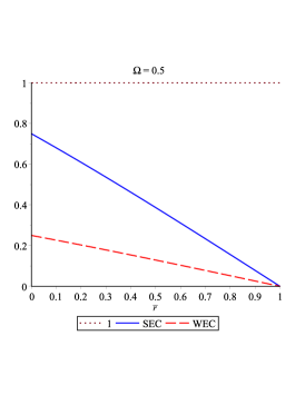
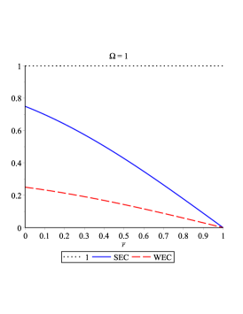
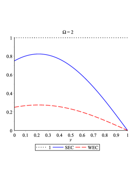
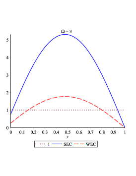
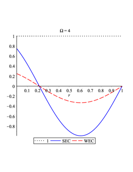
Figure 3: Diagrams for WEC and SEC inequalities for different values of the $\Omega$ parameter

We plot diagrams of the above inequalities in figure 3.

4.2 Regularity

By looking at the obtained density function (3.36) one can infer that it is convergent regular function for $0\leq\bar{r}\leq 1$. Furthermore arrow diagrams show that sink stable state for a regular visible stellar compact object with $a>0$ while for $a<0$ which is so called as dark stars the solutions has quasi stable nature in the arrow diagram and so one can infer that our obtained solutions behave same as stellar compact object with normal (non-dark) matter with positive barotropic index $a>0.$

4.3 Casuality

The speed of sound $v^{2}=\frac{dp}{d\rho}$ for a compact stellar object should be less than the speed of light $c=1$ and so by substituting the equation of state $p=a\rho^{2}$ one can obtain speed of sound for our model as

$$v=\sqrt{2a\rho}=\sqrt{\frac{\sin[\Omega(1-\bar{r})]}{2\Omega}}$$ (4.3)

which its diagram is plotted vs $\bar{r}$ for different values of the $\Omega$ parameter in figure 4-a. By looking at this diagram one can infer that the case $\Omega=4$ is not physical because does not satisfy the causality condition near the center $0<\bar{r}<0.2.$ In other words it is complex imaginary which is not seen in the diagram while other cases $0<\Omega<3$ satisfy the causality condition completely.

4.4 Stability

One of ways to check gravitational stability of a stellar system to be not collapsing is investigation of numeric values of the adiabatic index of the perfect fluid which in case of isotropic state is defined by $\Gamma=\frac{dp}{d\rho}(1+\rho/p)$ [37], [38] . When $\Gamma\geq\frac{4}{3}$ then a stellar fluid object is said to be stable from gravitational collapse. For our model one can show that

$$\Gamma=2(1+a\rho)\geq\frac{4}{3}$$ (4.4)

which means that our obtained solutions is free of gravitational collapse just for $a\rho\geq-\frac{1}{3}$ such that

$$\frac{\sin[\Omega(1-\bar{r})]}{4\Omega}\geq-\frac{1}{3}.$$ (4.5)

We plot diagram of this inequality for different values of the parameter $\Omega$ vs $0\leq\bar{r}\leq 1$ in figure 4-b. Other way to study stability of a compact gaseous stellar object in presence of radial perturbations was provided at a first time by Chandrashekhar (see [39] and [40]). It was developed and simplified by Harrison et al [41] and Zeldovich with collaboration of Novikov [42]. This is now well known as ‘Harrison-Zeldovich-Novikov (HZN) static stability criterion‘ which infers that any solution describes static and stable (unstable) stellar structure if the gravitational total mass $M(\rho(0))$ is an increasing (decreasing) function versus the central density $\rho(0)$ i.e, $\frac{\partial M}{\partial\rho(0)}>0(<0)$ under radial pulsations. For our model the HZN condition reads

$$HZN=\frac{1}{\sqrt{a}r_{c}^{2}}\frac{\partial M(\rho(0))}{\partial\rho(0)}=\frac{1}{\sin\Omega}\bigg{[}1-\bigg{(}\frac{\sin\Omega}{\Omega}\bigg{)}^{2}\bigg{]}$$ (4.6)

which we plot its diagram vs $\Omega$ in figure 4-c. It shows stability condition for choices $0<\Omega<\pi$ which obey the other diagrams given by figures 2. To see this one can look behavior of the red-dash-lines in figures 1-d, 2-a,2-b-2 and 2-c where the density functions take on positive values (NEC) for full interior region of the compact stellar object $0<\bar{r}<1$ but not for $\Omega=4$ given by the figure 2-d.

5 Conclusion

In this paper we considered a modified Einstein-Maxwell gravity where modification is the directional dependence of coupling between the electromagnetic field and Ricci tensor. Motivation of this kind of extensions is support of cosmic inflation with cosmic magnetic fields instead of unknown dark sector of the matter/energy. Hence we encouraged to investigate such a model for a stellar compact object system with a perfect fluid kind of matter source. To consider magnetic field of the model we use ansatz of magnetic field of magnetic monopole charge. We solved Tolman-Oppenheimer-Volkoff equation for interior metric of a spherically symmetric static perfect fluid. We used dynamical system approach to do because of nonlinearity form of the dynamical equations and obtained solutions of the fields near critical points. Our obtained solutions are physical because they satisfy energy conditions (NEC, WEC, SEC) and also the Harrison-Zeldovich-Novikov static stability. Also we check that sound speed is less than the light velocity and the obtained solutions obey the causality. In this work we use mean field theory approximation for matter stress tensor with mean energy density and isotropic pressure and we do not consider microscopic behavior of the matter source. As an extension of this work we like to study in our next work, effects of anisotropic imperfect fluid from point of view of its microscopic behavior in presence of magnetic monopole field.

Acknowledgement

This work was supported in part by the Semnan University Grant No. 1678-2021 for Scientific Research

6 Data Availability Statement

No Data associated in the manuscript

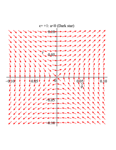
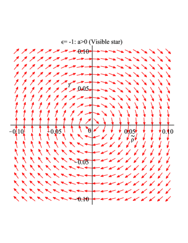
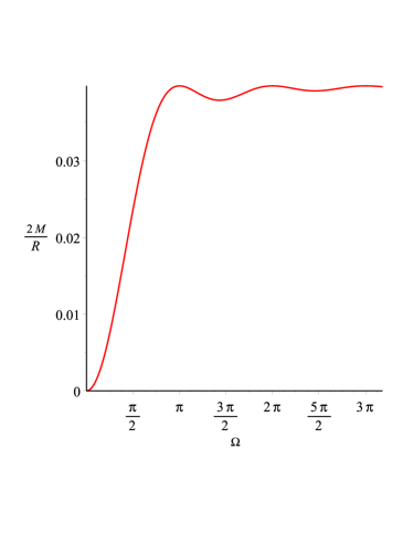
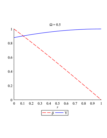
Figure 1: Arrow diagrams for dark sector of stellar object (Negative pressure $a<0$) (a) and visible stellar object (Positive pressure $a>0$) (b), Buchdahl inequality (compactness) parameter (c), density function $\bar{\rho}$ and metric field $Y$ for $\Omega=0.5$ (d)

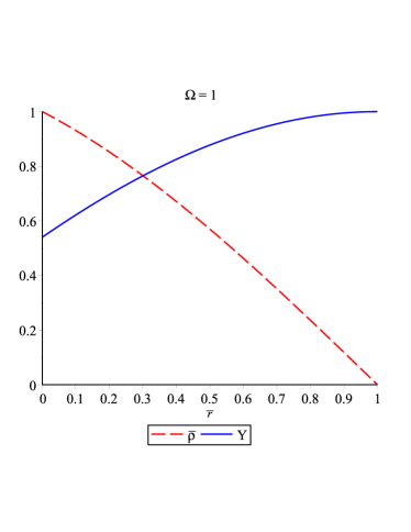
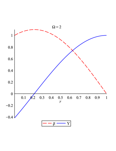
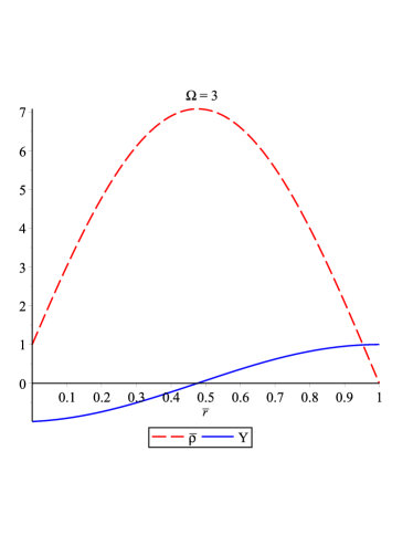
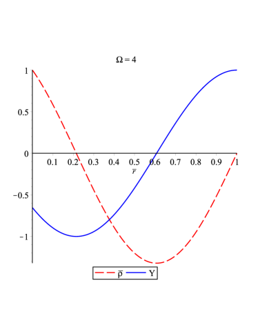
Figure 2: Diagrams of energy density and metric field for $\Omega=1$ (a), $\Omega=2$ (b), $\Omega=3$ (c) and $\Omega=4$ (d)

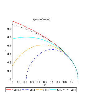
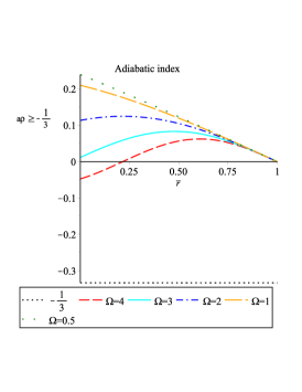
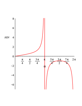
Figure 4: Diagrams for speed of sound (a) which is less than the light velocity describing a stable state. Diagram of adiabatic index (b) for which $a\rho\geq-\frac{1}{3}$ defines stabilization of the system.

References

- [1] J. Kumar and P. Bharti, ‘The classification of interior solutions of anisotropic fluid configurations‘, (2021), arXiv:2112.12518v2 [gr-qc]
- [2] P. Bhar, ‘Charged strange star with Krori Barua potential in f(R,T) gravity admitting Chaplygin equation of state‘, Eur. Phys. J. Plus 135, 757 (2020)
- [3] B. Dayanandan, S.K. Maurya and Smitha T. T,‘Modeling of charged anisotropic compact stars in general relativity‘, Eur. Phys. J. A 53, 141 (2017); arXiv:1611.00320 [gr-qc]
- [4] J. C. Jimnez and E. S. Fraga, ‘Radial oscillations in neutron stars from QCD‘, Phys. Rev. D 104, 014002 (2021); arXiv:2104.13480 [hep-ph]
- [5] F. Rocha, G. A. Carvalho, D. Deb and M. Malheiro, ‘Study of the charged super-Chandrasekhar limiting mass white dwarfs in the f(R,T) gravity‘,Phys. Rev. D 101, 104008 (2020); arXiv:1911.08894 [physics.gen-ph]
- [6] B. Kain, ‘Fermion-charged-boson stars‘, Phys. Rev. D 104, 043001 (2021); arXiv:2108.01404 [gr-qc]
- [7] X. Lai, Ch. Xia and R. Xu, ‘Bulk Strong Matter; the Trinity‘, ADVANCES IN PHYSICS, X, 8, 1, 2137433 (2023); arXiv: 2210.01501[hep-ph]
- [8] R. Kippnhahn, A. Weigret and A. Weiss, ‘Stellar Structure and Evolution‘ (Spriger-Verlag, Berlin Heidelberg, 2012).
- [9] P. L. Espino, V. Paschalidis, T. W. Baumgarte, and S. L. Shapiro, ‘Dynamical stability of quasitoroidal differentially rotating neutron stars‘, Phys. Rev. D 100, 043014 (2019).
- [10] R. S. Bogadi, M. Govender and S. Moyo,‘Dynamical (in)stability analysis of a radiating star model, cast from an initial static configuration‘, Eur. Phys. J. Plus. 135, 170 (2020).
- [11] J.H. Thomas and N. O. Weiss,‘Sunspots: Theory and Observations 139 (Springer Science+Business Media Dordrecht, 1992) .
- [12] C. Thompson, and R. C. Duncan, ‘The soft gamma repeaters as very strongly magnetized neutron stars I. Radiative mechanism for outbursts‘, MNRAS 275, 255 (1995).
- [13] C. Thompson C. and R. C. Duncan,‘The Soft Gamma Repeaters as Very Strongly Magnetized Neutron Stars. II. Quiescent Neutrino, X Ray, and Alfven Wave Emission‘APJ 473, 322 (1996).
- [14] J. MacDonald and D. J. Mullan,‘Magnetic fields in massive stars: dynamics and origin ‘ MNRAS 348, 702, (2004).
- [15] M. Gaurat, L. Jouve, F. Lignires and T. Gastine, ‘Evolution of a magnetic field in a differentially rotating radiative zone ‘,Astron. Astrophys. 580, A103 (2015).
- [16] D. Hooper, ‘Dark Cosmos: In Search of Our Universe’s Missing Mass and Energy‘, Harper Collins. ISBN:9780061976865, (2009).
- [17] S. Eidelman, K.G. Hayes, K.A. Olive, R.Y. Zhu ‘Review of Particle Physics‘, (Particle Data Group), Phys. Lett.B 592, 1 (2004) (URL: http://pdg.lbl.gov)
- [18] G. X. Wen, E. Witten, ‘Electric and magnetic charges in superstring models‘, Nucl. Phys. B, Vol261, 651 (2004).
- [19] S. Coleman, ‘ The Magnetic Monopole Fifty Years Later. In: Zichichi, A. (eds) The Unity of the Fundamental Interactions. Springer, Boston, MA.(1983), https://doi.org/10.1007/978-1-4613-3655-6-2
- [20] C. Castelnovo, R. Moessner and S. L. Sondhi, ‘Magnetic monopoles in spin ice‘, Nature 451,7174, 42 (2008); arXiv:0710.5515[cond-mat.str-el]
- [21] M. W. Ray, E. Ruokokoski, S. Kandel M. Mottonen and D. S. Hall, ‘Observation of Dirac monopoles in a synthetic magnetic field‘, Nature. 505, 7485, 657 (2014); arXiv:1408.3133[cond-mat.quant-gas]
- [22] P. Curie, ‘Sur la possibilite d’existence de la conductibilite magnetique et du magnetisme libre‘ [On the possible existence of magnetic conductivity and free magnetism]. Seances de la Societe Francaise de Physique (in French). Paris: 76, (1894).
- [23] P. Dirac, ‘Quantised Singularities in the Electromagnetic Field‘, Proc. Roy. Soc. (London) A 133, 60 (1931).
- [24] Lecture notes by Robert Littlejohn, University of California, Berkeley, 8 (2007)
- [25] P. B. Price, E.K. Shirk, W. Z. Osborne, and L. S. Pinsky, ‘Evidence for Detection of a Moving Magnetic Monopole‘, Phys. Rev. Lett. 35 (8), 487 (1975).
- [26] B. Cabrera, ‘First Results from a Superconductive Detector for Moving Magnetic Monopoles‘,Phys. Rev. Lett. 48 (20), 1378 (1982).
- [27] J. Polchinski, ‘Monopoles, Duality, and String Theory‘, Int. J. Mod. Phys. A. 19 (supp01), 145 (2004); arXiv:hep-th/0304042
- [28] T. D. Lee and Y. Pang, ‘Fermion soliton stars and black holes‘, Phys. Rev. D 35, 3678 (1987).
- [29] L. Del Grosso, G. Franciolini, P. Pani and A. Urbano, ‘Fermion Soliton Stars‘, arXiv:2301.08709 [gr-qc]
- [30] A. B. Balakin, V. V. Bochkarev and J. P. S. Lemos, ‘Non-minimal coupling for the gravitational and electromagnetic fields: black hole solutions and solitons‘, Phys.Rev.D77:084013,(2008); arXiv:0712.4066[gr-qc]
- [31] M. S. Turner, ‘Inflation-produced, large-scale magnetic fields‘, Phys. Rev. D 37, 2743 (1988)
- [32] N. K. Glendenning, ‘Compact Stars: Nuclear physics, Particle Physics, and general relativity‘, 2nd ed.(Springer, New York 2000)
- [33] J. Baez and J. P. Muniain, (‘Gauge Fields, Knots and Gravity‘, World Scientific publishing Co. Pte. Lid, 1994)
- [34] G. Arfken, ‘Mathematical methos for Physicists‘, Academic press Inc, (1985).
- [35] S. L. Liebling, L. Lehner, D. Neilsen and C. Palenzuela, ‘Evolution of magnetized and rotating neutron stars‘, Phys. Rev. D81, 124023 (2010).
- [36] H. Ghaffarnejad, E. Yaraie, ‘Dynamical system approach to scalar-vector-tensor cosmology‘,Gen Relativ Gravit 49, 49 (2017); arXiv:1604.06269 [physics.gen-ph]
- [37] V. Ferrari and M. Germano, ‘Scattering of gravitational waves by newotonian stars‘, Proc. R. Soc. Lond. A, 444, 389 (1994)‘
- [38] H. Hernandez, ‘Convection and cracking stability of spheres in General Relativity‘, Eur. Phys. J. C 78, 883 (2018); gr-qc/1808.10526
- [39] S. Chandrashekhar, ‘Dynamical Instability of Gaseous Masses Approaching the Schwarzschild Limit in General Relativity‘ Phys. Rev. Let,12,114,(1964);Erratum Phys. Rev. Lett. 12, 437 (1964)
- [40] S. Chandrashekhar, ‘The Dynamical Instability of Gaseous Masses Approaching the Schwarzschild Limit in General Relativity. ‘Astro. Phys. J. 140, 417 (1964).
- [41] B. K. Harrison et al, ‘Gravitational theory and Garavitational collapse‘, University of Chicago press, Chicago , (1966).
- [42] Y. B. Zeldovich and I. D. Novikov, ‘Relativity Astrophysical: Stars and Relativity‘, University of Chicago press, Chicago (1971).