Accelerating Antimicrobial Peptide Discovery with Latent Structure

Abstract.

Antimicrobial peptides (AMPs) are promising therapeutic approaches against drug-resistant pathogens. Recently, deep generative models are used to discover new AMPs. However, previous studies mainly focus on peptide sequence attributes and do not consider crucial structure information. In this paper, we propose a latent sequence-structure model for designing AMPs (LSSAMP). LSSAMP exploits multi-scale vector quantization in the latent space to represent secondary structures (e.g. alpha helix and beta sheet). By sampling in the latent space, LSSAMP can simultaneously generate peptides with ideal sequence attributes and secondary structures. Experimental results show that the peptides generated by LSSAMP have a high probability of antimicrobial activity. Our wet laboratory experiments verified that two of the 21 candidates exhibit strong antimicrobial activity. The code is released at https://github.com/dqwang122/LSSAMP.

1. Introduction

In recent years, the development of neural networks for drug discovery has attracted increasing attention. It can facilitate the discovery of potential therapies and reduce the time and cost of drug development (Stokes et al., 2020). Great success has been achieved in applying deep generative models to accelerate the discovery of potential drug-like molecules (Jin et al., 2018; Shi et al., 2019; Schwalbe-Koda and Gómez-Bombarelli, 2020; Xie et al., 2020).

Antimicrobial peptides (AMPs) are one of the most promising emerging therapeutic agents to replace antibiotics. They are short proteins that can kill bacteria by destroying the bacterial membrane (Aronica et al., 2021; Cardoso et al., 2020). Compared with the chemical interactions between antibiotics and bacteria that can be avoided by bacterial evolution, this physical mechanism is more difficult to resist.

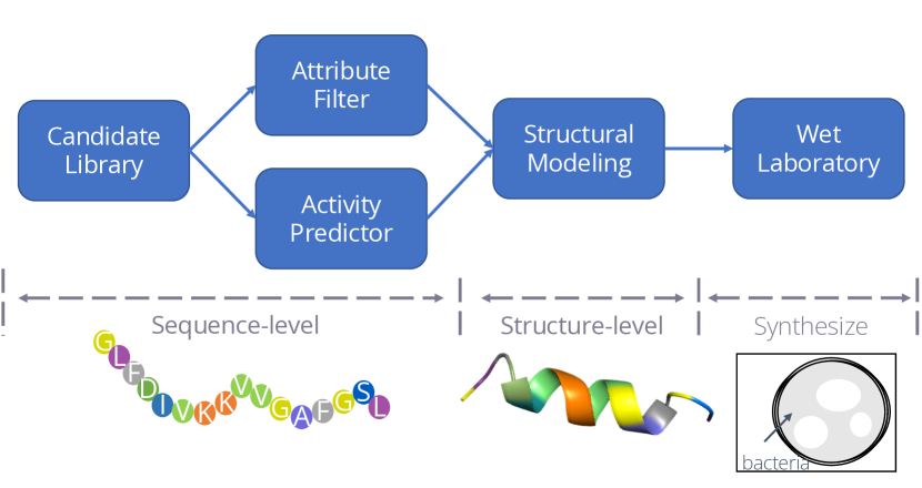
Figure 1. The overview of AMP discovery. The first two steps focus on sequence attributes and the third models the structure. The final step is to verify the antimicrobial activity by inhibiting the growth of bacteria. The grep region is the bacterial suspension and the white one means the bacteria concentration in this region is small.

A typical antimicrobial discovery process usually consists of four steps, as shown in Figure 1. First, a candidate library is built based on the existing AMPs database. These candidates can be created by applying manual heuristic approaches or training deep generative models. Then, several sequence-based filters are created to screen candidate peptides based on different chemical features, including computational metrics and predictive models trained to estimate ideal properties. After that, to ensure that these sequences can fold into appropriate structures with biological functions, the structure of these sequences will be modeled using peptide structure predictors such as PEPFold 3 (Shen et al., 2014) and molecule dynamics simulations will be performed. Finally, the filtered sequences will be synthesized and tested in the wet laboratory.

Recently, deep generative models have achieved great success in accelerating AMP discovery. They use sequence attributes to control the generation and directly generate peptides with ideal attributes directly (Das et al., 2018, 2021; Van Oort et al., 2021). However, these studies only consider sequence features and ignore the structure-activity relationship. The generated sequences still need to be fed into structure predictors and checked manually, which slows down the discovery process. Besides, the structure also plays an important role in determining biological attributes, which in turn facilitates attribute control (Chen et al., 2019; Torres et al., 2018; Tucker et al., 2018).

In this paper, we incorporate the structure information into the generative model and propose a Latent Sequence-Structure model for AntiMicrobial Peptide (LSSAMP). It maps the sequence features and secondary structures into the same latent space and samples the peptides with ideal sequence compositions and structures.LSSAMP controls the generation in a more fine-grained manner by assigning a latent variable to each position instead of a continuous variable to control the attributes of the whole sequence. We employ a multi-scale vector quantized-variational autoencoder (VQ-VAE) (van den Oord et al., 2017) to capture patterns of different lengths on sequences and structures. During the generation process, LSSAMP samples from the latent space and generates a peptide sequence with its secondary structure. The experimental results via public AMP predictors show that the peptides generated by LSSAMP have a high probability of AMP. We further conduct a comprehensive qualitative analysis, which indicates that our model captures the sequence and structure distribution. We select 21 generated peptides and conduct wet laboratory experiments, and find that 2 of them have high antimicrobial activity against Gram-negative bacteria.

To conclude, our contributions are as follows:

• We propose LSSAMP, a sequence-structure generative model that combines secondary structure information into the generation, which can further accelerate AMP discovery.

• We develop a multi-scale VQ-VAE to control the generation in a fine-grained manner and map patterns in sequences and structures into the same latent space.

• Experimental results of AMP predictors show that LSSAMP generates peptides with high probabilities of AMP. Moreover, 2 of 21 generated peptides show strong antimicrobial activities in wet laboratory experiments.

2. Related work

Antimicrobial Peptide Generation Traditional methods for AMP discovery can be divided into three approaches (Torres and de la Fuente-Nunez, 2019): (i) Pattern recognition algorithms first builds an antimicrobial sequential pattern database from existing AMPs. Each time a template peptide is chosen to substitute local fragments with those patterns (Loose et al., 2006; Porto et al., 2018). (ii) Genetic algorithms use the AMP database to design some antimicrobial activity functions and optimize ancestral sequences with these functions  (Maccari et al., 2013). (iii) Molecular modeling and molecular dynamics methods build 3D models of peptides and evaluate their antimicrobial activity by the interaction between peptides and the bacterial membrane (Matyus et al., 2007; Bolintineanu and Kaznessis, 2011). Pattern recognition and genetic algorithm bottleneck on representing patterns, and the modeling and dynamics method is computationally expensive and time-consuming.

Deep generative models take a rapid growth in recent years. Dean and Walper (2020) encodes the peptide into the latent space and interpolates across a predictive vector between a known AMP and its scrambled version to generate novel peptides. The PepCVAE (Das et al., 2018) and CLaSS (Das et al., 2021) employ the variational auto-encoder model to generate sequences. The AMPGAN (Van Oort et al., 2021) uses the generative adversarial network to generate new peptide sequences with a discriminator distinguishing the real AMPs and artificial ones. To our knowledge, this is the first study to incorporate secondary structure information into the generative phase, which is conducive to efficiently generating well-structured sequences with desired properties.

Sequence Generation via VQ-VAE The variational auto-encoders (VAEs) were first proposed by Kingma and Welling (2014) for image generation, and then widely applied to sequence generation tasks such as language modeling (Bowman et al., 2016), paraphrase generation (Gupta et al., 2018), machine translation (Bao et al., 2019) and so on. Instead of mapping the input to a continuous latent space in VAE, the vector quantized-variational autoencoder (VQ-VAE) (van den Oord et al., 2017) learns the codebook to obtain a discrete latent representation. It can avoid issues of posterior collapse while has comparable performance with VAEs. Based on it, Razavi et al. (2019) uses a multi-scale hierarchical organization to capture global and local features for image generation. Bao et al. (2021) learns implicit categorical information of target words with VQ-VAE and models the categorical sequence with conditional random fields in non-autoregressive machine translation. In this paper, we employ the multi-scale vector quantized technique to obtain the discrete representation for each position of the peptide.

3. Latent Sequence-Structure Model

In this section, we first introduce the background of AMP discovery and discuss the limitation of existing generative models. Then we introduce the Latent Sequence-Structure model for AMP (LSSAMP), which uses the multi-scale VQ-VAE to co-design sequence and secondary structure within the same latent space.

	Uniq	C	H	uH	Combination
VAE (Dean and Walper, 2020)	475	18.45% $\pm$ 2.92%	2.68% $\pm$ 3.28%	-2.78% $\pm$ 1.64%	0.29% $\pm$ 0.74%
AMP-GAN (Van Oort et al., 2021)	1966	2.79% $\pm$ 0.50%	2.16% $\pm$ 0.34%	-2.29% $\pm$ 0.53%	0.17% $\pm$ 0.35%
PepCVAE (Das et al., 2018)	208	3.87% $\pm$ 1.58%	-1.93% $\pm$ 1.61%	1.01% $\pm$ 2.80%	3.93% $\pm$ 1.82%
MLPeptide (Capecchi et al., 2021)	2106	-2.48% $\pm$ 0.39%	2.01% $\pm$ 0.57%	9.24% $\pm$ 1.22%	1.12% $\pm$ 0.38%

Table 1. The delta ratio of the sequence properties filtered by the secondary structures. Uniq is the uniq peptide number in 5000 generated sequences. C, H, uH correspond to charge, hydrophobicity, hydrophobic moment. Combination is the percentage of satisfying three valid ranges for AMPs at the same time.

3.1. Background

As shown in Figure 1, a typical AMP discovery includes the sequence-level attribute and the structure-level modeling before the wet laboratory experiments. Existing deep generative models have shown promise in accelerating AMP discovery by considering the sequence-level attributes during the generation. However, they still need to check and filter the structures with external tools after the sequence generation, which makes the process less efficient. For example, Van Oort et al. (2021) manually check the generated peptides and only got 12 AMP candidates with the ideal cationic and helical structure. Capecchi et al. (2021) required an extra secondary structure predictor (SPIDER3 (Heffernan et al., 2018)) to filter the generated peptides based on the percentage of the predicted a-helix structure fraction.

Moreover, there is a close relationship between the structure and activity of peptides. We investigate the effect of secondary structure on sequence properties by filtering the generated sequences based on the proportion of $\alpha$-helices, which is the most common secondary structure in AMPs. In Table 1, we use three sequence attributes (charge, hydrophobicity, hydrophobic moment) that are crucial for AMP mechanism to evaluate generation performance (Yeaman and Yount, 2003; Gidalevitz et al., 2003; Wimley, 2010).

The ratio in Table 1 is the difference in performance before and after the secondary structure filter. We can find that most of the results are improved by limiting alpha-helical structures. The results show that by controlling the structure, the sequence properties can be improved. Thus, incorporating the structure information into generative models can not only accelerate discovery by combining all the steps before the wet laboratory but also improve the sequence properties and make the generative process more efficient.

To address these challenges, we combine the secondary structure with sequence attributes in AMP discovery and generate peptides with ideal sequence attributes and secondary structures simultaneously.

Notation

A peptide with length $L$ can be denoted by $\mathbf{x}=\{x_{1},x_{2},\cdots,x_{L}\}$ and $x_{i}\in\mathcal{V}_{a}$ belongs to one of the 20 common amino acids, which is also called a residue. The secondary structure is used to describe the local form of the 3D structure of the peptide. It can be annotated as $\mathbf{y}=\{y_{1},y_{2},\cdots,y_{L}\}$, where $y_{i}\in\mathcal{V}_{s}$ is from 8 secondary structure types . The goal is to generate peptide candidates with high antimicrobial activities to accelerate the AMP discovery process.

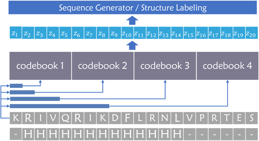
Figure 2. The encoder of LSSAMP. Here, we use $N=4$ pattern selectors to select local patterns with different scales and use the corresponding codebooks to obtain discrete latent variables $z_{i}$ for each position. The number of selectors is further discussed in Section 4.5.

3.2. VAE-based AMP Models

Given a sequence $\mathbf{x}$, the variational auto-encoders assume that it depends on a continuous latent variable $\mathbf{z}$. Thus the likelihood can be denoted by:

(1) $$p(\mathbf{x})=\int p(\mathbf{z})p(\mathbf{x}|\mathbf{z})d\mathbf{z}.$$

The controlled sequence generation incorporates the attribute $a$ and models the conditional probability $p(\mathbf{x}|a)$. Previous work such as PepCVAE (Das et al., 2018) assumes that $\mathbf{z}$ and $a$ are independent and $p(\mathbf{x}|a)=\int_{\mathbf{z}}p(\mathbf{z})p(\mathbf{x}|\mathbf{z},a)d\mathbf{z}$, while CLaSS (Das et al., 2021) models the dependency between $\mathbf{z}$ and $a$ by $p(\mathbf{x}|a)=\int_{\mathbf{z}}p(\mathbf{z}|a)p(\mathbf{x}|\mathbf{z})d\mathbf{z}$.

The vanilla VAE are usually trained in an auto-encoder framework with regularization. The encoder parameterizes an approximate posterior distribution $q_{\phi}(\mathbf{z}|\mathbf{x})$ and the decoder $p_{\theta}(\mathbf{x}|\mathbf{z})$ reconstructs $\mathbf{x}$ based on the latent $\mathbf{z}$. The models optimizes a evidence lower bound (ELBO):

(2) $$ELBO=E_{q_{\phi}(\mathbf{z}|\mathbf{x})}[log(p_{\theta}(\mathbf{x}|\mathbf{z}))]-\text{KL}(q_{\phi}(\mathbf{z}|\mathbf{x})||p(\mathbf{z})),$$

where the $E_{q_{\phi}(\mathbf{z}|\mathbf{x})}[log(p_{\theta}(\mathbf{x}|\mathbf{z}))]$ is the reconstruction loss and the KL divergence is the regularization. For the conditional generation, the attributes are directly fed to the decoder with latent variable $\mathbf{z}$ for $p_{\theta}(\mathbf{x}|\mathbf{z},a)$, or trained on the latent space to get an attribute-conditioned posterior distribution $p(\mathbf{z}|a)$. The VAE-based peptide generative models are first trained on the unsupervised peptide or protein sequences and then finetuned with a few sequences with biological attribute labels.

3.3. LSSAMP

To capture the sequence and the secondary structure feature simultaneously, we would like to model the joint distribution $p(\mathbf{x},\mathbf{y})$. Based on Eqn 2, the training objective is:

(3) $$ELBO=E_{q_{\phi}(\mathbf{z}|\mathbf{x},\mathbf{y})}[log(p_{\theta}(\mathbf{x},\mathbf{y}|\mathbf{z}))]-\text{KL}(q_{\phi}(\mathbf{z}|\mathbf{x},\mathbf{y})||p(\mathbf{z})).$$

For sequence $\mathbf{x}$ and secondary structure $\mathbf{y}$, we assume that they are independent given the latent variable $\mathbf{z}$. Thus the joint distribution can be written as $p(\mathbf{x},\mathbf{y})=\int_{z}p(\mathbf{x}|\mathbf{z})p(\mathbf{y}|\mathbf{z})p(\mathbf{z})d\mathbf{z}$. Moreover, since a peptide has a deterministic secondary structure given its amino acid sequence, we further approximate $q_{\phi}(\mathbf{z}|\mathbf{x},\mathbf{y})$ with $q_{\Phi}(\mathbf{z}|\mathbf{x})$. Therefore, the training objective is written as:

$$ELBO=E_{q_{\Phi}(\mathbf{z}|\mathbf{x})}[log(p_{\theta_{a}}(\mathbf{x}|\mathbf{z}))+log(p_{\theta_{s}}(\mathbf{y}|\mathbf{z}))]$$

(4) $$-\text{KL}(q_{\Phi}(\mathbf{z}|\mathbf{x})||p(\mathbf{z})).$$

For fine-grained control over each position, we assign one latent variable $z_{i}$ for each $x_{i}$ instead of a continuous $\mathbf{z}$ for the whole sequence. Since it is computationally intractable to sum continuous latent variables over the sequence, we use VQ-VAE (van den Oord et al., 2017) to lookup the discrete embedding vector $\mathbf{z}_{q}=\{z_{q}(x_{1}),\cdots,z_{q}(x_{L})\}$ for each position by vector quantization.

Specifically, the original latent variable $z_{e}(x_{i})\in\mathbb{R}^{d}$ will be replaced by the codebook entry $z_{q}(x_{i})\in\mathbb{R}^{d}$ via a nearest neighbors lookup from the codebook $\mathbf{B}\in\mathbb{R}^{K\times d}$ :

(5) $$z_{q}(x_{i})=e_{k},\text{and }k=\operatorname{argmin}_{j\in\{1,\cdots,K\}}\left\|{z_{e}(x_{i})-e_{j}}\right\|_{2}.$$

Here, $K$ is the slot number of the codebook and $d$ is the dimension of the codebook entry $e$. Then, the decoder will take $z_{q}(x_{i})$ as its input. So $\text{KL}(q_{\Phi}(\mathbf{z}|\mathbf{x})||p(\mathbf{z}))$ in Eqn 3.3 is replaced by:

(6) $$\left\|\operatorname{sg}\left[z_{e}(x_{i})\right]-z_{q}(x_{i})\right\|_{2}^{2}+\beta\left\|z_{e}(x_{i})-\operatorname{sg}[z_{q}(x_{i})]\right\|_{2}^{2},$$

measuring the difference between the original latent variable $z_{e}(x_{i})$ and the nearest codebook entry, rather than the KL divergence between two continuous distributions. Here, $sg(\cdot)$ is the stop gradient operator, which becomes 0 at the backward pass. $\beta$ is the commit coefficient to control the codebook loss.

For the sequence feature, we use the reconstruction loss to learn $\theta_{a}$, and for the secondary structure, we view it as an 8-category labeling task. Therefore, the first term in Eqn 3.3 becomes:

(7) $$\sum_{i=1}^{L}\log p_{\theta_{a}}\left(x_{i}|z_{q}(x_{i})\right)+\sum_{i=1}^{L}\log p_{\theta_{s}}\left(y_{i}|z_{q}(x_{i})\right)$$

However, the structure motifs are often longer than chain patterns. Therefore, we establish multiple codebooks to capture features of various scales.

Multi-scale VQ-VAE The structure motifs are often longer than sequence patterns. For example, a valid $\alpha$- helix contains at least 4 residues and may be longer than 12. However, sequence patterns with specific biological functions are much shorter, usually between 1 and 8 residues. In order to capture these features and map them into the same latent space, we first apply $N$ multi-scale pattern selectors $F_{n}$ on $z_{e}$ and get $z_{e_{n}}$. Then, we establish multiple codebooks $B_{n}\in\mathbb{R}^{K\times d}$ and use Eqn. 5 to look up the nearest codebook embedding $z_{q_{n}}(x_{i})$. We share the codebooks between sequence reconstruction and secondary structure prediction to capture common features and relationships between the residue and its structure. The concatenated multi-scale codebook embedding is fed to the sequence generator:

(8) $$z_{q}(x_{i})=\|_{n\in N}{z_{q_{n}}(x_{i})},$$

The total training objective is composed of the reconstruction loss, the labeling loss, and the codebook loss, which can be denoted by:

$$ELMO=\sum_{i=1}^{L}\log p_{\theta_{a}}\left(x_{i}|z_{q}(x_{i})\right)+\sum_{i=1}^{L}\log p_{\theta_{s}}\left(y_{i}|z_{q}(x_{i})\right)$$

(9) $$-\sum_{n=1}^{N}\left[\left\|\operatorname{sg}\left[z_{e_{n}}(x_{i})\right]-z_{q_{n}}(x_{i})\right\|_{2}^{2}+\beta\left\|z_{e_{n}}(x_{i})-\operatorname{sg}[z_{q_{n}}(x_{i})]\right\|_{2}^{2}\right]$$

The framework is shown in Figure 2.

Algorithm 1 Training and Sampling phase of LSSAMP

0:  A protein dataset $D_{r}$, a peptide dataset with secondary structure $D_{s}$, and the AMP dataset $D_{amp}$. The model $M$={$\theta_{a}$, $\theta_{s}$, $B_{n}$ } with $N$ codebooks. A set of $N$ prior models $M_{prior_{n}}$.

1:  Train on $D_{r}$ to optimize $\theta_{a}$ and $B_{n}$.

2:  Train on $D_{s}$ to optimize $\theta_{a}$, $\theta_{s}$, $B_{n}$ via Eqn. 3.3.

3:  Finetune $M$ on $D_{amp}$ via Eqn. 3.3.

4:  for  each codebook $n=1,2,\cdots,N$  do

5:     Create an empty dataset $C_{n}$.

6:     for $x_{i}\in D_{amp}$ do

7:        Get $n$-th codebook index $k_{i_{n}}$ of $x_{i}$ via Eqn. 5 and save it to $C_{n}$

8:     end for

9:     Train an auto-regressive language model $M_{\text{prior}_{n}}$ on $C_{n}$.

10:  end for

Training As VAE-based generative models, we first train LSSAMP in an unsupervised manner with protein sequences, which is similar to the original ELBO in Eqn 2. Then, we incorporate the structure information by jointly training on a smaller protein dataset with secondary structure annotation. Finally, we finetune our model on the AMP dataset to capture the specific AMP characteristics. The whole training process is described in Algorithm 1.

Following Kaiser et al. (2018), we use Exponential Moving Average (EMA) to update the embedding vectors in the codebooks. Specifically, we keep a count $c_{k}$ measuring the number of times that the embedding vector $e_{k}$ is chosen as the nearest neighbor of $z_{e}(x_{i})$ via Eqn. 5. Thus, the counts are updated with a sort of momentum: $c_{k}\leftarrow\lambda c_{k}+(1-\lambda)\sum_{i}\mathbb{I}[z_{q}(x_{i})=e_{k}]$, with the embedding $e_{k}$ being updated as $e_{k}\leftarrow\lambda e_{k}+(1-\lambda)\sum_{i}\frac{\mathbb{I}[z_{q}(x_{i})=e_{k}]z_{e}(x_{i})}{c_{k}}$. Here, $\lambda$ is the decay parameter.

Modeling dependency between position To model the dependency between $z_{1:L}$, we build an auto-regressive model on the index sequence of each codebook:

(10) $$p(\mathbf{z})=p(z_{1:L})=\prod_{i=1}^{L}p(z_{i}|z_{<i}).$$

Specifically, we train Transformer-based language models $M_{\text{prior}_{n}}$ based on the index sequences from Eqn. 5 for each codebook $n$ .

Sampling We sample several index sequences from the prior models for each codebook $n$, and then look up the codebook to get the embedding vector $\mathbf{z}_{q_{n}}$. Finally, $\mathbf{z}_{q_{n}}$ is fed to the decoder to generate the sequence with its secondary structure. We also further control the secondary structure by heuristic structure patterns to improve the generation quality.

4. Experiment

We first describe our experiment settings (Section 4.1) and introduce the automatic evaluation metrics (Section 4.2) and results (Section 4.3). Then, we verify the antimicrobial activity in the wet laboratory (Section 4.4). Last but not least, we conduct an in-depth analysis (Section 4.5) to understand LSSAMP and discuss its limitation (Section 4.6).

	SVM	RF	DA	Scanner	AMPMIC	IAMPE	amPEP	Average
APD	87.78%	91.24%	86.24%	94.66%	98.42%	97.83%	91.50%	92.52%
Decoy	17.43%	13.71%	16.04%	0.25%	18.07%	23.53%	52.92%	20.28%
Random $p=0.1$	86.06%	86.12%	84.01%	93.23%	79.14%	95.60%	91.74%	87.99%
Random $p=0.2$	76.66%	76.64%	74.83%	86.95%	68.57%	91.14%	87.89%	80.38%
VAE (Dean and Walper, 2020)	24.90%	15.30%	13.83%	15.12%	15.25%	40.31%	24.30%	21.29%
AMP-GAN (Van Oort et al., 2021)	78.62%	87.29%	83.82%	82.17%	89.58%	93.88%	80.52%	85.13%
PepCVAE (Das et al., 2018)	82.84%	85.96%	93.33%	85.44%	98.44%	98.14%	80.77%	89.27%
MLPeptide (Capecchi et al., 2021)	90.43%	92.55%	93.08%	93.72%	96.34%	97.05%	91.37%	93.51%
LSSAMP	92.03%	92.60%	93.45%	91.52%	95.84%	96.64%	93.23%	93.62%
LSSAMP w/o cond	78.98%	80.24%	80.01%	86.73%	83.81%	93.80%	85.32%	84.13%

Table 2. The percentage of generated sequences being predicted as AMP. The classifiers are described in Section 4.2.1. The first part is the prediction results on AMP and non-AMP dataset as the reference. The bold ones are the best model results.

4.1. Experiment Setup

Dataset The Universal Protein Resource (UniProt) is a comprehensive protein dataset. We download reviewed protein sequences (550k) with the limitation of 100 in length as $D_{r}$ (57k examples). Then we use a community reimplementation of AlphaFold(AlQuraishi, 2019), which is called ProSPr (Billings et al., 2019) to predict the secondary structure for $D_{r}$. After filtering some low-quality examples, we obtain $D_{s}$ with 46k examples, including both sequence and secondary structure information. For the antimicrobial peptide dataset, we download from Antimicrobial Peptide Database (APD) (Wang et al., 2016) and filter repeated ones to get 3222 AMPs as $D_{amp}$. We randomly extract 3,000 examples as validation and 3,000 as the test on $D_{r}$ and $D_{s}$. For $D_{amp}$, the size of validation and test is both 100. Following Veltri et al. (2018), we create a decoy set of negative examples without antimicrobial activities for comparison. It removes peptide sequences with antimicrobial activity from Uniprot, and sequences with length $<10$ or $>40$, resulting in 2021 non-AMP sequences (Decoy).

Baseline Traditional methods usually randomly replace several residues on existing AMPs and conduct biological experiments on them. Thus, we use Random baseline to represent the method of replacing residue randomly with a probability $p$. Following Dean and Walper (2020), we use VAE to embed the peptides into the latent space and sample latent variable $z$ from the standard Gaussian distribution $p\sim N(0,1)$. For a fair comparison, we use the same Transformer architecture as our model LSSAMP and train on the Uniprot $D_{r}$ and APD dataset $D_{amp}$. AMP-GAN is proposed by Van Oort et al. (2021), which uses a BiCGAN architecture with convolution layers. It consists of three parts: the generator, discriminator, and encoder. The generator and discriminator share the same encoder. It is trained on 49k false negative sequences from UniProt and 7k positive AMP sequences. PepCVAE is a semi-VAE generative model that concatenates the attribute features to the latent variable for conditional generation (Das et al., 2018). Since the authors did not release their code, we use the model architecture from Hu et al. (2017) and modify the reproduced code for AMPs, as described in their paper. The original paper uses 93k sequences from UniProt and 7960/6948 positive/negative AMPs for training. For comparison, we use UniProt dataset $D_{r}$ and ADP dataset $D_{amp}$ to train it. MLPeptide (Capecchi et al., 2021) is RNN-based generator. It is first trained on 3580 AMPs and then transferred to specific bacteria. LSSAMP is implemented as described in Section 3.3 and the detailed hyperparameters are attached in Appendix A.3.

4.2. Automatic Evaluation Metric

Following previous work (Das et al., 2020; Van Oort et al., 2021), we use open-source AMP prediction tools to estimate the AMP probability of the generated sequence. Since these open-source AMP predictors are trained and report results in different AMP datasets, we use them to predict sequences in APD and decoy datasets as a reference of their performance. We also evaluate the generative diversity of these models.

	Uniq	C	H	uH	Combination
APD	3222	68.75%	27.96%	4.72%	6.15%
Decoy	2020	21.83%	8.81%	1.98%	0.10%
Random $p=0.1$	4978	65.86% $\pm$ 0.19%	26.80% $\pm$ 0.23%	23.10% $\pm$ 0.58%	4.38% $\pm$ 0.16%
Random $p=0.2$	5000	62.13% $\pm$ 0.39%	24.87% $\pm$ 0.29%	20.79% $\pm$ 0.76%	2.47% $\pm$ 0.17%
VAE	4988	38.00% $\pm$ 0.36%	21.07% $\pm$ 0.58%	12.43% $\pm$ 0.66%	0.34% $\pm$ 0.11%
AMP-GAN	4976	87.66% $\pm$ 0.45%	17.31% $\pm$ 0.74%	23.45% $\pm$ 0.73%	1.92% $\pm$ 0.05%
PepCVAE	1346	15.61% $\pm$ 0.06%	14.54% $\pm$ 0.55%	11.65% $\pm$ 0.23%	2.75% $\pm$ 0.25%
MLPeptide	4486	77.95% $\pm$ 0.72%	8.11% $\pm$ 0.27%	32.91% $\pm$ 0.60%	2.90% $\pm$ 0.16%
LSSAMP	4876	81.88% $\pm$ 0.31%	25.06% $\pm$ 0.45%	37.10% $\pm$ 0.33%	6.26% $\pm$ 0.07%
LSSAMP w/o cond	4903	82.04% $\pm$ 0.42%	21.32% $\pm$ 0.34%	30.51% $\pm$ 0.51%	4.46% $\pm$ 0.20%

Table 3. Sequence attributes of generated sequences. We use the percentage of peptides meeting the valid range (Appendix A.1) to measure the performance. Uniq is the number of unique generated sequences. C, H, uH correspond to charge, hydrophobicity, hydrophobic moment. The best results are bold.

4.2.1. AMP Classifiers

Thomas et al. (2010) trained on the AMP database of 3782 sequences with random forest (RF), discriminant analysis (DA), support vector machines (SVM), and artificial neural network (ANN) respectively. AMP Scanner v2 (Veltri et al., 2018), short as Scanner, is a CNN-&LSTM-based deep neural network trained on 1778 AMPs picked from APD. AMPMIC (Witten and Witten, 2019) trained a CNN-based regression model on 6760 unique sequences and 51345 MIC measurement to predict MIC values. IAMPE (Kavousi et al., 2020) is a model based on Xtreme Gradient Boosting. It achieves the highest correct prediction rate on a set of ten more recent AMPs (Aronica et al., 2021). ampPEP (Lawrence et al., 2021) is a random forest based model which is trained on 3268 AMPs. It has the best performance across multiple datasets (Aronica et al., 2021).

4.2.2. Sequence Attributes

Following the previous AMP design (Das et al., 2018; Van Oort et al., 2021; Capecchi et al., 2021; Das et al., 2021), we use the three sequence attributes to evaluate the generation performance: Charge(C), Hydrophobicity(H), Hydrophobic Momentum (uH). Here, we use $x_{i}$ to denote the $i$-th residue and $S$ to indicate the sequence.

Charge is important because the bacterial membrane usually takes the negative charge and peptides with the positive charge are more likely to bind with the membrane. We only take integer charges into consideration. The whole charge of the peptide sequence $S$ is defined as the sum of the charge of all its residues $C(x_{i})$ at pH 7.4, which is $C(S)=\sum_{x_{i}\in S}{C(x_{i})}$.

Hydrophobicity reflects the tendency to bind lipids on the bacterial membrane. A peptide with a high hydrophobicity is easy to move from the solution environment to the bacterial membrane.We use the hydrophobicity scale $H(x_{i})$ in Eisenberg et al. (1984) to calculate the hydrophobicity of a sequence, which is $H(S)=\sum_{x_{i}\in S}{H(x_{i})}$.

Hydrophobic Momentum. It is viewed as the measure of amphipathicity, indicating the ability of the peptide to bind water and lipid simultaneously. It is a definitive feature of antimicrobial peptides(Hancock and Rozek, 2002). Hydrophobic momentum $uH(S,\theta)$ is defined by Eisenberg et al. (1984). The hydrophobic momentum is determined by the hydrophobicity $H(x_{i})$ of each residue $x_{i}$, along with the angle $\theta$ between residues. The angle can be estimated by the secondary structure. $\theta$ is $100^{\circ}$ for the $\alpha$-helix structure, and $180^{\circ}$ for $\beta$-sheet.

(11) $$uH(S,\theta)=\sqrt{R_{cos}^{2}(S,\theta)+R_{sin}^{2}(S,\theta)},$$

(12) $$R_{cos}(S,\theta)=\sum_{x_{i}\in S}{H(x_{i})*cos(i*\theta)},$$

(13) $$R_{sin}(S,\theta)=\sum_{x_{i}\in S}{H(x_{i})*sin(i*\theta)}.$$

For each peptide, we calculate the above attributes to measure its antimicrobial activity. For comparison, we draw the distribution on the APD and decoy dataset and select a range for each attribute based on the biological mechanism (Appendix A.1). We use the percentage of peptides in each attribute range to exploit the generation performance and use Combination to measure the percentage of peptides that satisfy three conditions at the same time.

4.2.3. Novelty

To measure the novelty of the generated peptides, we define three evaluation metrics: Uniqueness, Diversity, and Similarity. Uniqueness is the percentage of unique peptides in the generation phase. Diversity measures the similarity among the generated peptides. We calculate the Levenshtein distance (Levenshtein et al., 1966) between every two sequences and normalize it by the sequence length. Then we average the normalized distance to get the mean as its diversity. The higher the diversity, the more dissimilar the generated peptides are. Novelty is the difference between the generated peptides and the training AMP set. For each generated sequence, we search the training set for a peptide that has the smallest Levenshtein distance from it and normalizes the distance according to its length. We calculate the average length as the Novelty.

	Uniqueness $\uparrow$	Diversity $\uparrow$	Novelty $\uparrow$
Random $p=0.1$	0.995 $\pm$ 0.000	0.871 $\pm$ 0.021	0.078 $\pm$ 0.001
Random $p=0.2$	0.999 $\pm$ 0.000	0.971 $\pm$ 0.022	0.160 $\pm$ 0.001
VAE	0.986 $\pm$ 0.001	1.011 $\pm$ 0.038	0.584 $\pm$ 0.002
AMP-GAN	0.995 $\pm$ 0.001	0.907 $\pm$ 0.023	0.565 $\pm$ 0.007
PepCVAE	0.265 $\pm$ 0.006	0.367 $\pm$ 0.007	0.423 $\pm$ 0.005
MLPeptide	0.900 $\pm$ 0.003	0.850 $\pm$ 0.016	0.416 $\pm$ 0.010
LSSAMP	0.981 $\pm$ 0.001	0.878 $\pm$ 0.018	0.503 $\pm$ 0.005
LSSAMP w/o cond	0.976 $\pm$ 0.002	0.901 $\pm$ 0.013	0.515 $\pm$ 0.008

Table 4. The novelty of the sampling. $\uparrow$ means higher is better.

	PPL $\downarrow$	Loss $\downarrow$	AA Acc.$\uparrow$	SS Acc.$\uparrow$
LSSAMP	3.24 $\pm$ 0.16	1.17 $\pm$ 0.05	99.79 $\pm$ 0.20	87.20 $\pm$ 0.62
w/o $D_{r}$	11.56 $\pm$ 3.81	2.45 $\pm$ 0.94	66.06$\pm$ 0.67	82.78 $\pm$ 0.57
w/o $D_{s}$	3.83 $\pm$ 0.32	1.34 $\pm$ 0.04	99.58$\pm$ 0.26	85.87$\pm$ 0.35
w/o subbook	3.49 $\pm$ 0.20	1.25 $\pm$ 0.05	99.86 $\pm$ 0.36	86.61 $\pm$ 0.95

Table 5. Ablation Study on validation set of $D_{amp}$. ‘w/o’ indicates that we remove the module from LSSAMP. $\uparrow$ means higher is better, and $\downarrow$ is the opposite.

No	Sequence	Activity (ug/mL) $\downarrow$			Sequence identity $\downarrow$	Hemolysis/Toxicity $\downarrow$
		A. Baumannii	P. aeruginose	E. coli
P1	GAFGNFLKNVAKKAGIYLLSIAQCKLFGTP	16-32	/	32-64	83.30%	Low
P2	FIGFLFKLAKKIIPSLFQTKTE	8	32	/	75.00%	Low

Table 6. Wet laboratory experiment results. The activity is measured by MIC and $\downarrow$ means the lower the better. ‘Sequence identity’ measures the similarity with existing AMPs and ‘Hemolysis/Toxicity’ measures the damage to other cells.

4.3. Experimental Results

We generate 5000 sequences for each baseline. During the generation process, we add structural restrictions on positions based on the antimicrobial mechanism. Specifically, we reject peptides with more than 30% coil structure (‘-’), which can hardly fold in the solution environment, and insert the bacterial membrane in silico screening. Besides, we limit the minimum length of a continuous helix (‘H’) to 4 according to physical rules. We name our model with structural control as LSSAMP and the model without extra conditions as LSSAMP w/o cond.

AMP Prediction The results of prediction tools are shown in Table 2. LSSAMP performs best in four of seven and has the highest average score across all classifiers, indicating its advantage over baselines. PepCVAE performs best on the AMPMIC and IAMPE predictors, however, it performs poorly on the other predictors and gets a low average score. MLPeptide performs relatively evenly across predictors, outperforming other models on only Scanner and slightly underperforming our model on the average score. The comparison of LSSAMP and LSSAMP w/o cond indicates that adding fine-grained control on the secondary structure can further improve the generation performance. It further indicates the importance of taking the secondary structure into consideration during the AMP generation.

Sequence Attributes As listed in Table 3, LSSAMP outperforms all baselines on the combination percentage, which indicates that our model can generate sequences satisfying multiple properties at the same time. Besides, the combination percentage is similar to APD, which means that our model generates sequences that have a similar distribution to APD. LSSAMP tends to generate peptides with higher hydrophobicity, while AMP-GAN and MLPeptide sample more cationic sequences. It is because they were only trained on sequences and more focused on the direct amino acid attributes. Compared with them, LSSAMP can better capture the amphiphilic indicated by the highest uH for the incorporation of structure labels. PepCVAE inefficiently generates redundant sequences, which results in a significant decrease in the number of unique sequences. Since the percentage is calculated based on the whole generation size (5000), it leads to low performance on all attributes. Furthermore, we can find that by further controlling the secondary structure, H, uH and Combination can be improved. This verifies that secondary structure will also affect sequence attributes.

Novelty From Table 4, we can see that VAE has the highest diversity and novelty. However, from Table 2 and Table3, we can find that the peptides generated by VAE do not have a high probability of AMP or the ideal sequence attributes. It means that the vanilla VAE trained on AMP datasets without attribute control can hardly capture the antimicrobial features. At the same time, LSSAMP has a significant advantage over the above strong baseline PepCVAE and MLPeptide. It means that our model can generate promising AMPs with relatively high novelty. Besides, the limitation of the secondary structure will lead to a decline in diversity. However, it does not result in more redundant peptides because the uniqueness does not decrease. It indicates that the restrictions make the model capture similar local patterns, but not generate the exact same sequence.

Codebook	PPL $\downarrow$	Loss $\downarrow$	AA Acc.$\uparrow$	SS Acc.$\uparrow$
$[1]$	19.04 $\pm$ 2.84	2.94 $\pm$ 0.14	65.49 $\pm$ 3.49	83.41 $\pm$ 2.34
$[1,2]$	3.84 $\pm$ 0.09	1.35 $\pm$ 0.02	99.40 $\pm$ 0.45	85.39 $\pm$ 0.26
$[1,2,4]$	3.32 $\pm$ 0.03	1.20 $\pm$ 0.01	100.00 $\pm$ 0.00	85.95 $\pm$ 0.42
$[1,2,4,8]$	3.24 $\pm$ 0.16	1.17 $\pm$ 0.05	99.79 $\pm$ 0.20	87.20 $\pm$ 0.62

Table 7. The influence of the number of codebooks on validation set of $D_{amp}$. ‘[1,2,4,8]’ indicates that we use 4 codebooks with window sizes of 1,2,4,8. The meanings of symbols are the same as Table 5.

Ablation Study We conduct the ablation study for our LSSAMP and show the results in Table 5. PPL is the perplexity of generated sequences that can measure fluency. Loss is the model loss on the validation set. AA Acc. is the reconstruction accuracy of residue and SS Acc. is the prediction accuracy of the secondary structure. We can find that without the first training phase on $D_{r}$, the model can hardly generate valid sequences. The second phase to train the model on the large-scale secondary structure dataset $D_{s}$ will affect the prediction performance on the target AMP dataset. If we remove multiple sub-codebooks and use a single large codebook with the same size, the performance will also decline.

4.4. Wet Laboratory Experiments

We synthesized and experimentally characterize peptides designed with LSSAMP. First, we filtered the 5000 generated peptide sequences based on their physical attributes (as outlined in Section 4.2.2 and Appendix A.1) and employed off-the-shelf AMP classifiers to select the ones with high antimicrobial scores (as detailed in Section 4.2.1). Second, we rank the sequences according to their novelty (as described in Section 4.2.3) and select ones with edit distance greater than 5 residues from the existing training sequences. Finally, we obtained 21 peptides and synthesized them for wet-lab experiments.

Following the previous AMP design (Capecchi et al., 2021; Das et al., 2021), we use minimum inhibitory concentration (MIC) to indicate peptide activity, which is defined as the lowest concentration of an antibiotic that prevents the visible growth of bacteria. A lower MIC means a higher antimicrobial activity. To determine MIC, the broth microdilution method was used. A colony of bacteria was grown in LB (Lysogeny broth) medium overnight at 37 degrees under PH=7. A peptide concentration range of 0.25 to 128 mg/liter was used for MIC assay. The concentration of bacteria was quantified by measuring the absorbance at 600 nm and diluted to OD600 = 0.022 in MH medium. The sample solutions(150uL) were mixed with a 4uL diluted bacterial suspension and finally inoculated with about 5 * 10E5 CFU. The Plates were incubated at 37 degrees until satisfactory growth  18h. For each test, two columns of plates were reserved for sterile control (broth only) and growth control (broth with bacterial inoculum, no antibiotics). The MIC was defined as the lowest concentration of the peptide dendrimer that inhibited the growth of bacteria visible after treatment with MTT.

We tested their antimicrobial activities against three panels of Gram-negative bacteria (A. Baumannii, P. aeruginose, E. coli), which cost about 30 days. As shown in Table 6, two peptides were both found to be effective against A. Baumannii. P2 against P. aeruginose and P1 against for E.coli also showed activity. Besides, these two newly discovered AMPs differ from existing AMPs and had low toxicity, which means they are promising new therapeutic agents. The wet-lab experiment results demonstrate LSSAMP can effectively find AMP candidates and reduce the time.

ID	Sequence	Secondary Structure	C	H	uH
Y1	FLPLVRVWAKLI	–HHHHHHHHHH	2.0	0.471	0.723
Y2	FLSTVPYVAFKVVPTLFCPIAKTC	–HHHHHHHHHHHHHHHHHHHT–	2.0	0.446	1.812
Y3	FFGVLARGIKSVVKHVMGLLMG	–HHHHHHHHHHHHHHHHHH–	3.0	0.420	0.549
Y4	GVLPAFKQYLPGIMKIIVKF	–HHHHHHHHHHHHHHH—	3.0	0.419	0.523
Y5	VFTLLGAIIHHLGNFVKRFSHVF	-HHHHHHHHHHHHHHHHHHHH–	2.0	0.416	0.514
Y6	FVPGLIKAAVGIGYTIFCKISKACYQ	–HHHHHHHHHHHHHHHHHHHT—-	3.0	0.394	1.815
Y7	ALWCQMLTGIGKLAGKA	–HHHHHHHHHHHHHHH	2.0	0.344	0.506
Y8	LLTRIIVGAISAVTSLIKKS	–HHHHHHHHHHHHHHHH–	3.0	0.334	0.531
Y9	FLSVIKGVWAASLPKQFCAVTAKC	–HHHHHHHHHHHHHHHHHHHT–	3.0	0.334	0.660
Y10	FLNPIIKIATQILVTAIKCFLKKC	–HHHHHHHHHHHHHHHHHHHT–	4.0	0.334	1.940

Table 8. 10 generated peptides. ‘H’ is the alpha-helix, ‘T’ is the Turn and ‘-’ is the coil.

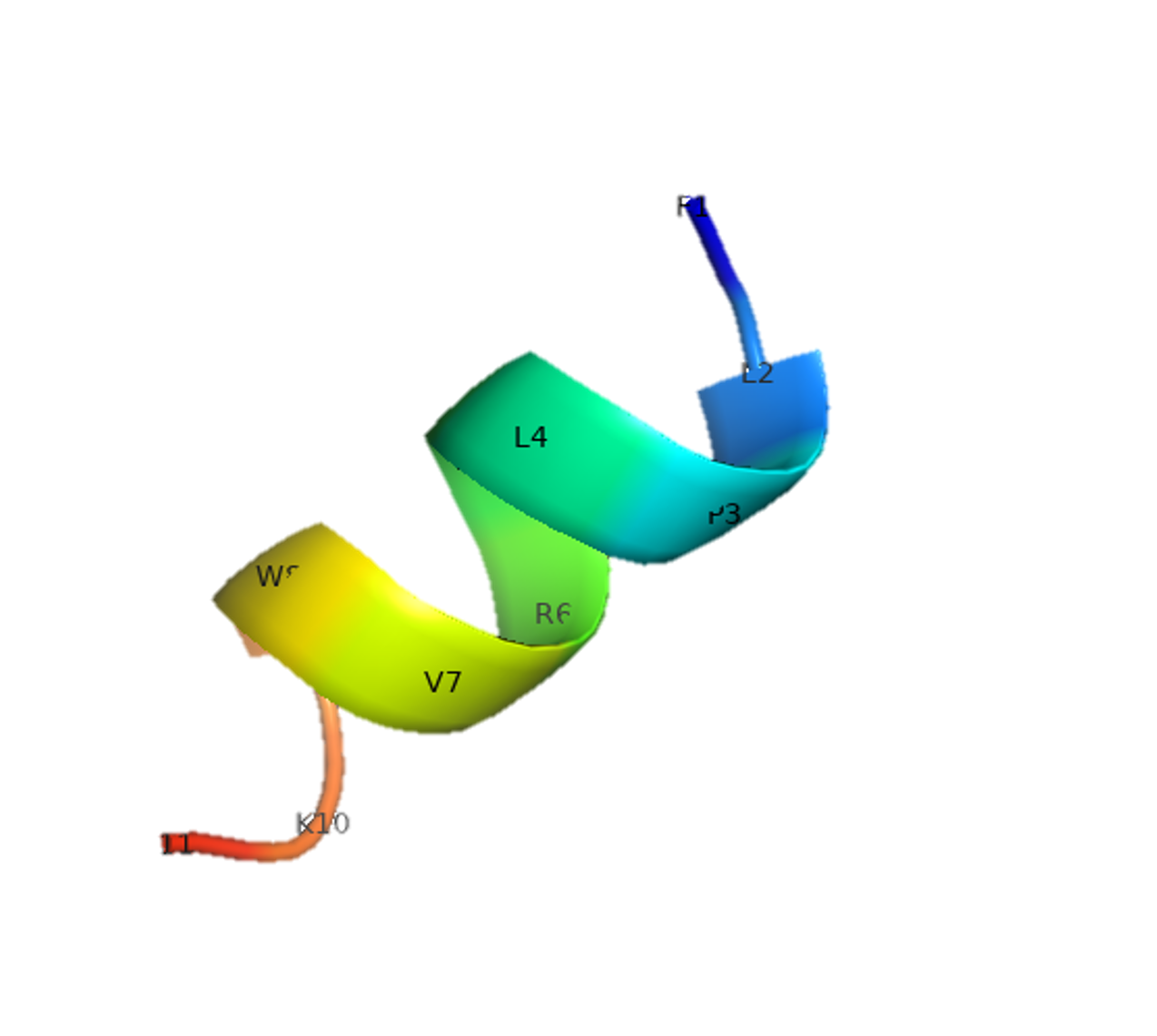
(a) Y1

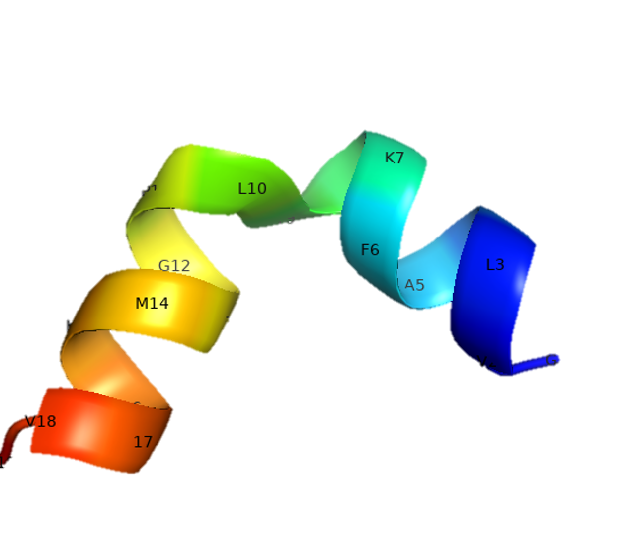
(b) Y4

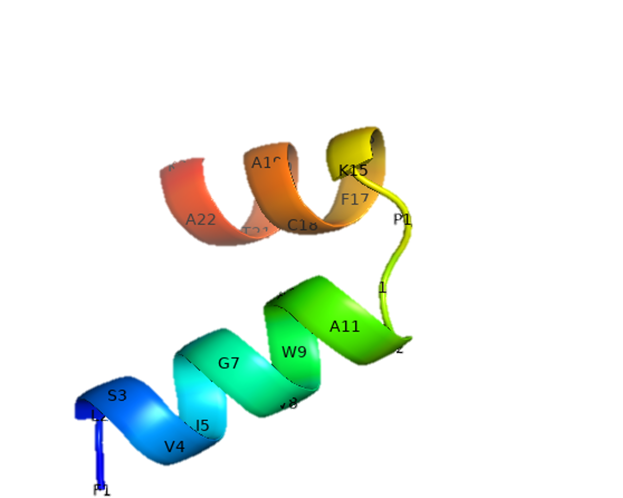
(c) Y9

(d) Y10

Figure 3. 3D structures for Y1, Y4, Y9, and Y10 in Table 8.

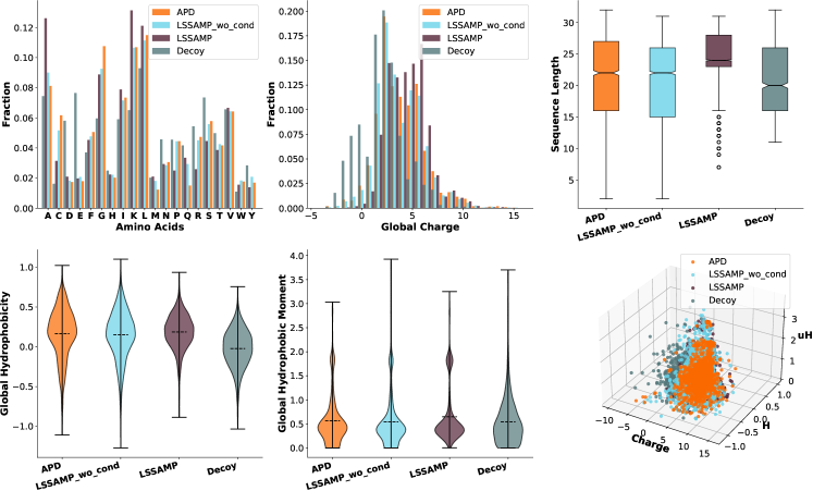
Figure 4. The distribution of amino acids, charge, sequence length, hydrophobicity, hydrophobic momentum, and a 3D visualization for three sequence attributes.

4.5. Analysis

Codebook Number We explore the effect of different numbers of codebooks on generation performance. From Table 7, we find that a single small codebook can hardly learn enough information to reconstruct the sequence. The PPL, Loss, and SS Acc. become better with the increase of codebook entries. However, the reconstruction accuracy achieves the best performance when the codebook is 3. This may be due to the relatively short local pattern of sequences, making the window of 8 too long for it. We do not increase the window size to $[1,2,4,8,16]$ because the maximum length of the sequence has been set to 32, making 16 too long to capture features.

Case Study We show 10 peptides generated by LSSAMP in Table 8. We can see that all of them have long alpha-helix in the middle and coil structures at the head or tail. We can also find that these sequences have positive charges with high hydrophobicity and hydrophobicity momentum. We further predict and build 3D structures of 4 generated sequences via PEPFold 3 (Shen et al., 2014) and draw the image via PyMOL (Schrödinger, LLC, 2015) in Figure 3. We can find that all these four peptides have helical structures, which is consistent with our secondary structure prediction. These helical structures make them more likely to have the antimicrobial ability. However, our model also fails for predicting a long continuous helical structure for Y4 and Y9. In fact, they have a small coil structure between the two helical structures. It indicates that our model tends to predict a long continuous secondary structure instead of several discontinuous small fragments.

Visualization of LSSAMP Distribution We plot the distribution of residues, charge, sequence length, hydrophobicity, and hydrophobic momentum for APD, Decoy, and LSSAMP and LSSAMP w/o cond in Figure 4. For the distribution of amino acids, the x-axis is different amino acids and the y-axis is their frequency in the generation set. We can find that without the extra condition, LSSAMP w/o cond has a similar amino acid distribution with APD. However, when we add the secondary structure conditions, it will greatly increase the frequency of A, K, and L. And we can find that those amino acids have a relatively high distribution in APD, which means that they might be responsible for the antimicrobial activity. Therefore, the addition of secondary structures may further change the direction of amino acid distribution to increase the probability of becoming AMPs.

For the global charge, we can find that compared with APD, the decoy dataset has more negative-charge sequences. And our models tend to generate sequences with positive charges. In the sequence length, we can find that the control of structure makes the length of generated sequence less diverse and tends to be longer. This is because we forced the generated sequences to have an alpha-helix structure of a length of more than 4. In hydrophobicity and hydrophobic momentum, we can find a similar tendency where the LSSAMP w/o cond captures the distribution of APD, and the secondary structure condition makes the distribution more concentrated with a higher mean.

In the 3D visualization, we use the charge, H, and uH as the axes to see the combination of the three attributes. We can see that LSSAMP and LSSAMP w/o cond are almost overlapped by APD, which indicates that these three have a similar distribution on these attributes. Decoy sequences are out of the scope.

To conclude, Figure 4 is a sanity check indicating our base model LSSAMP w/o cond can successfully capture the distribution of APD from various dimensions, and the extra secondary structure condition will further improve the distribution.

4.6. Limitation

Although LSSAMP has shown its effectiveness, it is limited by several factors. First, LSSAMP models the secondary structure instead of the 3D structure. The use of 3D structures is limited by the size of the available precise data and the difficulty of predicting 3D structures with only one input sequence. Compared to 3D structures, secondary structures are much easier to annotate. Benefiting from the development of AlphaFold2 in predicting 3D structures, we expect to further extend the work and incorporate the 3D information into the latent representation space and generate sequences with ideal 3D structures.

The other limitation is that currently there is no standard evaluation metric for antimicrobial activities. In this paper, we follow the previous practice of using AMP classifiers and sequence properties to evaluate performance. However, the performance of AMP classifiers on generated peptides may be unreliable because they are trained on existing AMPs (Aronica et al., 2021). Furthermore, it is difficult to identify a reasonable range of sequence properties. It is because existing AMPs have different mechanisms that result in various sequence attributes. The only reliable evaluation method to check antimicrobial activity is the wet laboratory test, but it is expensive and time-consuming, which makes it impossible to perform a large number of evaluations. In the future, we hope that more reliable automatic evaluation metrics for AMPs will be proposed.

5. Conclusion

In this paper, we propose LSSAMP that jointly learns sequential and structural features in the same latent space and can generate peptides with ideal sequence attributes and secondary structures simultaneously. Moreover, It leverages multi-scale VQ-VAE for fine-grained control of each position. The performance evaluated using open resource AMP predictors and computational sequence attributes indicates the effectiveness of LSSAMP. It further designs two peptides with high activity against Gram-negative bacteria. This suggests that our generative model can effectively create an AMP library with high-quality candidates for follow-up biological experiments, which can accelerate the AMP discovery.

Appendix A Appendix

A.1. Attribute Distribution

To determine the effective threshold of charge, hydrophobicity, and hydrophobic moment of AMP, we analyze the sequence distribution in APD and decoy in Figure 5. For charge, we follow the rule summarized by experts and choose sequences whose net charge is +2 to +10. For the remaining two characters, we draw a histogram and compare the proportion in each box. If the proportion of APD is larger than that in the decoy, we add bin to the acceptance range of the evaluation metric. The final ranges are $C\in[2,10]$, $H\in[0.25,\infty]$, and $uH\in[0.5,0.75]\cup[1.75,\infty]$.

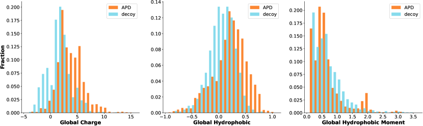
Figure 5. The histogram of charge, hydrophobicity and hydrophobic moment on APD and decoy dataset.

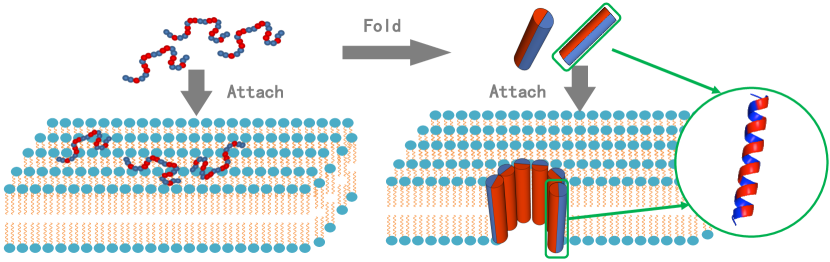
Figure 6. An example of the antimicrobial mechanism. The blue indicates the hydrophobic amino acids, and the red ones are hydrophilic. On the left, although the peptides with reasonable amino acids have attached to the bacterial membrane, they still can not insert into it. However, by folding into the helix structure, as shown on the right, the peptides maintain a stable hole that breaks the membrane of the bacterium.

	Uniq	C	H	uH	Combination
Random $p=0.1$	2055	7.38% $\pm$ 11.01%	37.93% $\pm$ 0.44%	4.61% $\pm$ 0.31%	4.34% $\pm$ 0.41%
Random $p=0.2$	1831	6.87% $\pm$ 0.31%	9.52% $\pm$ 0.31%	1.91% $\pm$ 1.06%	2.19% $\pm$ 0.66%
VAE (Dean and Walper, 2020)	475	18.45% $\pm$ 2.92%	2.68% $\pm$ 3.28%	-2.78% $\pm$ 1.64%	0.29% $\pm$ 0.74%
AMP-GAN (Van Oort et al., 2021)	1966	2.79% $\pm$ 0.50%	2.16% $\pm$ 0.34%	-2.29% $\pm$ 0.53%	0.17% $\pm$ 0.35%
PepCVAE (Das et al., 2018)	208	3.87% $\pm$ 1.58%	-1.93% $\pm$ 1.61%	1.01% $\pm$ 2.80%	3.93% $\pm$ 1.82%
MLPeptide (Capecchi et al., 2021)	2106	-2.48% $\pm$ 0.39%	2.01% $\pm$ 0.57%	9.24% $\pm$ 1.22%	1.12% $\pm$ 0.38%
LSSAMP	4876	0.30% $\pm$ 0.37%	3.96% $\pm$ 0.64%	7.53% $\pm$ 0.41%	1.87% $\pm$ 0.07%

Table 9. The delta ratio of sequence properties filtered by secondary structures. Uniq is the uniq peptide number among 5000 generated sequences. C, H, uH correspond to charge, hydrophobicity, hydrophobic moment. Combination is the percentage satisfying three ranges at the same time.

A.2. Secondary Structure Filter

Similar to proteins, the biological functions of AMPs are determined by their amino acid sequences and folded structures (Boman, 2003). If the peptide can not fold into an appropriate structure, it is still difficult to take effect. For example, by forming a helical structure, the peptide can gather hydrophobic amino acids on one side and hydrophilic amino acids on the other. This amphiphilic structure helps the peptide insert into the membrane and maintain a stable hole with other molecules in the membrane, as shown in Figure 6. Without it, the peptide can hardly penetrate the membrane and attach to the surface.

But does controlling secondary structure also affect sequence attributes? To answer this question, we control the secondary structure of the generated peptides to $\alpha$-helix for our baseline. The performance gaps are shown in Table 9. From Table 9, we can find that most of the results are improved by limiting sequences to the $\alpha$-helix structures. It shows that by controlling the structure, the sequence attributes can be improved, which verifies the importance of introducing secondary structures to the controlled generation process. However, the sequence size has decreased significantly, indicating that this generate-then-filter pipeline is inefficient.

Visualization of Residue Distribution

To illustrate the distribution of residues in the generated peptides, we plot tSNE, shown in Figure 7. We transform the vector with each dimension representing the probability of a certain residue to represent the peptide. Then we use tSNE to convert the high-dimensional vector to 2D and visualize them. We find that there is a large overlap between LSSAMP w/o condition and APD, which indicates that our model has captured the global distribution of APD instead of collapsing to a local mode. Furthermore, LSSAMP covers APD and has some outliers. The results show that with the secondary structure condition, our model can not only learn the existing AMP distribution but also explore more possible spaces.

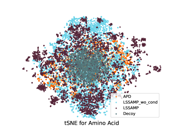
Figure 7. The tSNE plot for the distribution of residue in each sequence on four datasets.

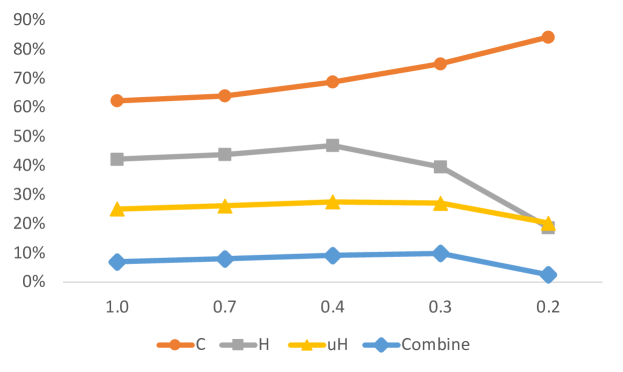
Figure 8. The sequence attributes of peptides with different percentages of the coil structure. The x-axis is the maximum percentage and the y-axis is the percentage of peptides that meet the attribute range.

Structure Condition

As described above, controlling the secondary structure can affect the attributes of generated peptides. Thus we limit the percentage of the coil structure with different ratios and calculate the sequence attributes of generated peptides. The results are shown in Figure 8. The x-axis is the maximum percentage of the coil structures allowed during the generation. We can find that with the decrease in the length of coil structures, the percentage of positive peptides keeps growing. However, for hydrophobicity and hydrophobic momentum, the percentage drop after 0.3. Therefore, we limit the length of the coil structure to 30% in our main experiments.

A.3. Implementation

Implementation details There are three main modules for LSSAMP. The encoder and decoder are based on a 2-layer Transformer (Vaswani et al., 2017) with $d_{model}=128$, $head=8$. The size of FFN projection is $d_{ffn}=512$ and all drouput rate are $0.1$. For the classifier, we use the same CNN block as Billings et al. (2019) with 32 input channels and a dilation scale of $[1,2,4,8,10]$. For multi-scale codebooks, we first apply CNN to extract features. We set $n=4$ and kernel width ranging in $[1,2,4,8]$. The features will be padded to the same length as the input sequence. Then, we use 4 codebooks with $K=8$ and $d=128$. The reconstruction and prediction share the same codebooks, which means $N_{r}=N_{s}=4$. The commit coefficient is set to $\beta=0.05$.

Reproduction We run the model several times and calculate the mean and variance of the main experimental results and analysis. We use PyTorch to implement our model and train it on a single Tesla-V100-32GB. We optimize the parameter with Adam Optimizer (Kingma and Ba, 2015). During pre-training for sequence construction on $D_{r}$, we set the maximum token in a batch $bz$ as 30,000, learning rate $lr$ as 0.01 with 8,000 warm-up steps, and decoy weight for EMA as $\lambda=0.8$. For secondary structure prediction on $D_{s}$, the max length is limited to 32, $bz=10,000$, $lr=0.003$, $\lambda=0.95$, and the prediction loss coefficient $\gamma=1$. Finally, we transfer to $D_{amp}$ with the same hyperparameters except the $lr=0.001$.

A.4. More Case Study

Disulfide Bonds

Studies have shown that disulfide bonds also contribute to the native-folded AMP stability and affect the activity of AMPs by influencing their folding stability (Nehls et al., 2020; Deplazes et al., 2020). Therefore, we also manually check the disulfide bonds in Table 8. For disulfide bonds, there should be at least two Cys residues, so Y2, Y6, Y9, and Y10 are likely to form disulfide bonds. Therefore, we also model 3D structure of Y2 and Y6 in Figure 9. The Y9 and Y10 are shown in Figure 3. For Y6, Y9, and Y10, at least one of the Cys residues lies on the alpha-helix and does not form the disulfide bond. For Y2, the Cys residues don’t form any stable structure. This is no surprise because we control the generated peptide to form the helix structure. Meanwhile, our model fails in predicting the coil and beta structure in Y2, which illustrates the limitation of our secondary structure modeling.

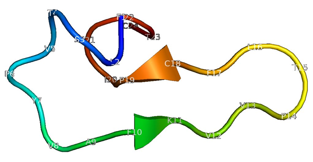
(a) Y2

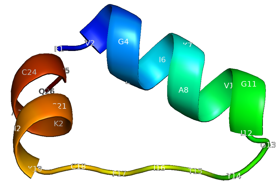
(b) Y6

Figure 9. 3D structures for Y1 and Y6 in Table 8.

References

- (1)
- AlQuraishi (2019) Mohammed AlQuraishi. 2019. AlphaFold at CASP13. Bioinformatics 35, 22 (2019), 4862–4865.
- Aronica et al. (2021) Pietro GA Aronica, Lauren M Reid, Nirali Desai, Jianguo Li, Stephen J Fox, Shilpa Yadahalli, Jonathan W Essex, and Chandra S Verma. 2021. Computational Methods and Tools in Antimicrobial Peptide Research. Journal of Chemical Information and Modeling 61, 7 (2021), 3172–3196.
- Bao et al. (2021) Yu Bao, Shujian Huang, Tong Xiao, Dongqi Wang, Xinyu Dai, and Jiajun Chen. 2021. Non-Autoregressive Translation by Learning Target Categorical Codes. In Proc. of NAACL-HLT. 5749–5759.
- Bao et al. (2019) Yu Bao, Hao Zhou, Shujian Huang, Lei Li, Lili Mou, Olga Vechtomova, Xinyu Dai, and Jiajun Chen. 2019. Generating Sentences from Disentangled Syntactic and Semantic Spaces. In Proc. of ACL.
- Billings et al. (2019) Wendy M Billings, Bryce Hedelius, Todd Millecam, David Wingate, and Dennis Della Corte. 2019. ProSPr: democratized implementation of alphafold protein distance prediction network. bioRxiv (2019), 830273.
- Bolintineanu and Kaznessis (2011) Dan S Bolintineanu and Yiannis N Kaznessis. 2011. Computational studies of protegrin antimicrobial peptides: a review. Peptides 32, 1 (2011), 188–201.
- Boman (2003) HG Boman. 2003. Antibacterial peptides: basic facts and emerging concepts. Journal of internal medicine 254, 3 (2003), 197–215.
- Bowman et al. (2016) Samuel R Bowman, Luke Vilnis, Oriol Vinyals, Andrew M Dai, Rafal Jozefowicz, and Samy Bengio. 2016. Generating sentences from a continuous space. In 20th SIGNLL Conference on Computational Natural Language Learning, CoNLL 2016. Association for Computational Linguistics (ACL), 10–21.
- Capecchi et al. (2021) Alice Capecchi, Xingguang Cai, Hippolyte Personne, Thilo Kohler, Christian van Delden, and Jean-Louis Reymond. 2021. Machine Learning Designs Non-Hemolytic Antimicrobial Peptides. Chemical Science (2021).
- Cardoso et al. (2020) Marlon H Cardoso, Raquel Q Orozco, Samilla B Rezende, Gisele Rodrigues, Karen GN Oshiro, Elizabete S Cândido, and Octávio L Franco. 2020. Computer-aided design of antimicrobial peptides: are we generating effective drug candidates? Frontiers in microbiology 10 (2020), 3097.
- Chen et al. (2019) Charles H Chen, Charles G Starr, Evan Troendle, Gregory Wiedman, William C Wimley, Jakob P Ulmschneider, and Martin B Ulmschneider. 2019. Simulation-guided rational de novo design of a small pore-forming antimicrobial peptide. Journal of the American Chemical Society 141, 12 (2019), 4839–4848.
- Das et al. (2021) Payel Das, Tom Sercu, Kahini Wadhawan, Inkit Padhi, Sebastian Gehrmann, Flaviu Cipcigan, Vijil Chenthamarakshan, Hendrik Strobelt, Cicero Dos Santos, Pin-Yu Chen, et al. 2021. Accelerated antimicrobial discovery via deep generative models and molecular dynamics simulations. Nature Biomedical Engineering 5, 6 (2021), 613–623.
- Das et al. (2020) Payel Das, Tom Sercu, Kahini Wadhawan, Inkit Padhi, Sebastian Gehrmann, Flaviu Cipcigan, Vijil Chenthamarakshan, Hendrik Strobelt, Cicero dos Santos, Pin-Yu Chen, et al. 2020. Accelerating Antimicrobial Discovery with Controllable Deep Generative Models and Molecular Dynamics. arXiv preprint arXiv:2005.11248 (2020).
- Das et al. (2018) Payel Das, Kahini Wadhawan, Oscar Chang, Tom Sercu, Cicero Dos Santos, Matthew Riemer, Vijil Chenthamarakshan, Inkit Padhi, and Aleksandra Mojsilovic. 2018. Pepcvae: Semi-supervised targeted design of antimicrobial peptide sequences. arXiv preprint arXiv:1810.07743 (2018).
- Dean and Walper (2020) Scott N Dean and Scott A Walper. 2020. Variational autoencoder for generation of antimicrobial peptides. ACS omega 5, 33 (2020), 20746–20754.
- Deplazes et al. (2020) Evelyne Deplazes, Yanni K-Y Chin, Glenn F King, and Ricardo L Mancera. 2020. The unusual conformation of cross-strand disulfide bonds is critical to the stability of -hairpin peptides. Proteins: Structure, Function, and Bioinformatics 88, 3 (2020), 485–502.
- Eisenberg et al. (1984) David Eisenberg, Robert M Weiss, and Thomas C Terwilliger. 1984. The hydrophobic moment detects periodicity in protein hydrophobicity. Proceedings of the National Academy of Sciences 81, 1 (1984), 140–144.
- Gidalevitz et al. (2003) David Gidalevitz, Yuji Ishitsuka, Adrian S Muresan, Oleg Konovalov, Alan J Waring, Robert I Lehrer, and Ka Yee C Lee. 2003. Interaction of antimicrobial peptide protegrin with biomembranes. Proceedings of the National Academy of Sciences 100, 11 (2003), 6302–6307.
- Gupta et al. (2018) Ankush Gupta, Arvind Agarwal, Prawaan Singh, and Piyush Rai. 2018. A Deep Generative Framework for Paraphrase Generation. In Proc. of AAAI, Sheila A. McIlraith and Kilian Q. Weinberger (Eds.). 5149–5156.
- Hancock and Rozek (2002) Robert EW Hancock and Annett Rozek. 2002. Role of membranes in the activities of antimicrobial cationic peptides. FEMS microbiology letters 206, 2 (2002), 143–149.
- Heffernan et al. (2018) Rhys Heffernan, Kuldip Paliwal, James Lyons, Jaswinder Singh, Yuedong Yang, and Yaoqi Zhou. 2018. Single-sequence-based prediction of protein secondary structures and solvent accessibility by deep whole-sequence learning. Journal of computational chemistry 39, 26 (2018), 2210–2216.
- Hu et al. (2017) Zhiting Hu, Zichao Yang, Xiaodan Liang, Ruslan Salakhutdinov, and Eric P Xing. 2017. Toward controlled generation of text. In International Conference on Machine Learning. PMLR, 1587–1596.
- Jin et al. (2018) Wengong Jin, Kevin Yang, Regina Barzilay, and Tommi Jaakkola. 2018. Learning Multimodal Graph-to-Graph Translation for Molecule Optimization. In International Conference on Learning Representations.
- Kabsch and Sander (1983) Wolfgang Kabsch and Christian Sander. 1983. Dictionary of protein secondary structure: pattern recognition of hydrogen-bonded and geometrical features. Biopolymers: Original Research on Biomolecules 22, 12 (1983), 2577–2637.
- Kaiser et al. (2018) Lukasz Kaiser, Samy Bengio, Aurko Roy, Ashish Vaswani, Niki Parmar, Jakob Uszkoreit, and Noam Shazeer. 2018. Fast decoding in sequence models using discrete latent variables. In International Conference on Machine Learning. PMLR, 2390–2399.
- Kavousi et al. (2020) Kaveh Kavousi, Mojtaba Bagheri, Saman Behrouzi, Safar Vafadar, Fereshteh Fallah Atanaki, Bahareh Teimouri Lotfabadi, Shohreh Ariaeenejad, Abbas Shockravi, and Ali Akbar Moosavi-Movahedi. 2020. IAMPE: NMR-assisted computational prediction of antimicrobial peptides. Journal of Chemical Information and Modeling 60, 10 (2020), 4691–4701.
- Kingma and Ba (2015) Diederik P. Kingma and Jimmy Ba. 2015. Adam: A Method for Stochastic Optimization. In Proc. of ICLR, Yoshua Bengio and Yann LeCun (Eds.).
- Kingma and Welling (2014) Diederik P Kingma and Max Welling. 2014. Auto-Encoding Variational Bayes. (2014).
- Lawrence et al. (2021) Travis J Lawrence, Dana L Carper, Margaret K Spangler, Alyssa A Carrell, Tomás A Rush, Stephen J Minter, David J Weston, and Jessy L Labbé. 2021. amPEPpy 1.0: a portable and accurate antimicrobial peptide prediction tool. Bioinformatics 37, 14 (2021), 2058–2060.
- Levenshtein et al. (1966) Vladimir I Levenshtein et al. 1966. Binary codes capable of correcting deletions, insertions, and reversals. In Soviet physics doklady, Vol. 10. Soviet Union, 707–710.
- Loose et al. (2006) Christopher Loose, Kyle Jensen, Isidore Rigoutsos, and Gregory Stephanopoulos. 2006. A linguistic model for the rational design of antimicrobial peptides. Nature 443, 7113 (2006), 867–869.
- Maccari et al. (2013) Giuseppe Maccari, Mariagrazia Di Luca, Riccardo Nifosí, Francesco Cardarelli, Giovanni Signore, Claudia Boccardi, and Angelo Bifone. 2013. Antimicrobial peptides design by evolutionary multiobjective optimization. PLoS computational biology 9, 9 (2013), e1003212.
- Matyus et al. (2007) Edit Matyus, Christian Kandt, and D Peter Tieleman. 2007. Computer simulation of antimicrobial peptides. Current medicinal chemistry 14, 26 (2007), 2789–2798.
- Nehls et al. (2020) Christian Nehls, Arne Böhling, Rainer Podschun, Sabine Schubert, Joachim Grötzinger, Andra Schromm, Henning Fedders, Matthias Leippe, Jürgen Harder, Yani Kaconis, et al. 2020. Influence of disulfide bonds in human beta defensin-3 on its strain specific activity against Gram-negative bacteria. Biochimica et Biophysica Acta (BBA)-Biomembranes 1862, 8 (2020), 183273.
- Porto et al. (2018) William F Porto, Isabel CM Fensterseifer, Suzana M Ribeiro, and Octavio L Franco. 2018. Joker: An algorithm to insert patterns into sequences for designing antimicrobial peptides. Biochimica et Biophysica Acta (BBA)-General Subjects 1862, 9 (2018), 2043–2052.
- Razavi et al. (2019) Ali Razavi, Aaron van den Oord, and Oriol Vinyals. 2019. Generating diverse high-fidelity images with vq-vae-2. In Advances in neural information processing systems. 14866–14876.
- Schrödinger, LLC (2015) Schrödinger, LLC. 2015. The PyMOL Molecular Graphics System, Version 1.8. (November 2015).
- Schwalbe-Koda and Gómez-Bombarelli (2020) Daniel Schwalbe-Koda and Rafael Gómez-Bombarelli. 2020. Generative models for automatic chemical design. In Machine Learning Meets Quantum Physics. Springer, 445–467.
- Shen et al. (2014) Yimin Shen, Julien Maupetit, Philippe Derreumaux, and Pierre Tuffery. 2014. Improved PEP-FOLD approach for peptide and miniprotein structure prediction. Journal of chemical theory and computation 10, 10 (2014), 4745–4758.
- Shi et al. (2019) Chence Shi, Minkai Xu, Zhaocheng Zhu, Weinan Zhang, Ming Zhang, and Jian Tang. 2019. GraphAF: a Flow-based Autoregressive Model for Molecular Graph Generation. In International Conference on Learning Representations.
- Stokes et al. (2020) Jonathan M Stokes, Kevin Yang, Kyle Swanson, Wengong Jin, Andres Cubillos-Ruiz, Nina M Donghia, Craig R MacNair, Shawn French, Lindsey A Carfrae, Zohar Bloom-Ackermann, et al. 2020. A deep learning approach to antibiotic discovery. Cell 180, 4 (2020), 688–702.
- Thomas et al. (2010) Shaini Thomas, Shreyas Karnik, Ram Shankar Barai, Vaidyanathan K Jayaraman, and Susan Idicula-Thomas. 2010. CAMP: a useful resource for research on antimicrobial peptides. Nucleic acids research 38, suppl_1 (2010), D774–D780.
- Torres et al. (2018) Marcelo DT Torres, Cibele N Pedron, Yasutomi Higashikuni, Robin M Kramer, Marlon H Cardoso, Karen GN Oshiro, Octavio L Franco, Pedro I Silva Junior, Fernanda D Silva, Vani X Oliveira Junior, et al. 2018. Structure-function-guided exploration of the antimicrobial peptide polybia-CP identifies activity determinants and generates synthetic therapeutic candidates. Communications biology 1, 1 (2018), 1–16.
- Torres and de la Fuente-Nunez (2019) Marcelo Der Torossian Torres and Cesar de la Fuente-Nunez. 2019. Toward computer-made artificial antibiotics. Current opinion in microbiology 51 (2019), 30–38.
- Tucker et al. (2018) Ashley T Tucker, Sean P Leonard, Cory D DuBois, Gregory A Knauf, Ashley L Cunningham, Claus O Wilke, M Stephen Trent, and Bryan W Davies. 2018. Discovery of next-generation antimicrobials through bacterial self-screening of surface-displayed peptide libraries. Cell 172, 3 (2018), 618–628.
- van den Oord et al. (2017) Aaron van den Oord, Oriol Vinyals, and Koray Kavukcuoglu. 2017. Neural discrete representation learning. In Proceedings of the 31st International Conference on Neural Information Processing Systems. 6309–6318.
- Van Oort et al. (2021) Colin M Van Oort, Jonathon B Ferrell, Jacob M Remington, Safwan Wshah, and Jianing Li. 2021. AMPGAN v2: Machine Learning-Guided Design of Antimicrobial Peptides. Journal of Chemical Information and Modeling (2021).
- Vaswani et al. (2017) Ashish Vaswani, Noam Shazeer, Niki Parmar, Jakob Uszkoreit, Llion Jones, Aidan N. Gomez, Lukasz Kaiser, and Illia Polosukhin. 2017. Attention is All you Need. In Proc. of NeurIPS, Isabelle Guyon, Ulrike von Luxburg, Samy Bengio, Hanna M. Wallach, Rob Fergus, S. V. N. Vishwanathan, and Roman Garnett (Eds.). 5998–6008.
- Veltri et al. (2018) Daniel Veltri, Uday Kamath, and Amarda Shehu. 2018. Deep learning improves antimicrobial peptide recognition. Bioinformatics 34, 16 (2018), 2740–2747.
- Wang et al. (2016) Guangshun Wang, Xia Li, and Zhe Wang. 2016. APD3: the antimicrobial peptide database as a tool for research and education. Nucleic acids research 44, D1 (2016), D1087–D1093.
- Wimley (2010) William C Wimley. 2010. Describing the mechanism of antimicrobial peptide action with the interfacial activity model. ACS chemical biology 5, 10 (2010), 905–917.
- Witten and Witten (2019) Jacob Witten and Zack Witten. 2019. Deep learning regression model for antimicrobial peptide design. BioRxiv (2019), 692681.
- Xie et al. (2020) Yutong Xie, Chence Shi, Hao Zhou, Yuwei Yang, Weinan Zhang, Yong Yu, and Lei Li. 2020. MARS: Markov Molecular Sampling for Multi-objective Drug Discovery. In International Conference on Learning Representations.
- Yeaman and Yount (2003) Michael R Yeaman and Nannette Y Yount. 2003. Mechanisms of antimicrobial peptide action and resistance. Pharmacological reviews 55, 1 (2003), 27–55.