Energy supply into a semi-infinite $\beta$-Fermi-Pasta-Ulam-Tsingou chain by periodic force loading

Abstract

We deal with dynamics of the $\beta$-Fermi-Pasta-Ulam-Tsingou chain with one free end, subjected to the sinusoidal periodic force. We examine evolution of the total energy, supplied at large times. In the harmonic case ($\beta=0$), the energy grows in time linearly at non-zero group velocities, corresponding to the excitation frequency and grows in time as $\sqrt{t}$ at zero group velocity. Explanation of behavior in time of the energy is proposed by analysis of obtained approximate closed-form expression for the field of particle velocities. In the weak anharmonic case, large-time asymptotic approximation for the total energy is obtained by using the renormalized dispersion relation. Operating of the approximation, we analyze energy transfer at the driving frequencies, lying both in the pass-band and in the stop-band of the harmonic chain. Consistency of the asymptotic assesses with the results of numerical simulations is discussed.

1 Introduction

Investigation of response of a medium under external excitation is one among the oldest engineering problems, with which one has been encountered [1, 2]. Nowadays the problem concerns not merely the macroscale, but rather the micro- and nanoscale, wherein one deals with discrete structures (see, e.g., [3, 4]).

Wave transmission into the discrete linear medium is known to be possible only at driving frequencies, enclosed inside the pass-band. In contrast, energy can propagate into the nonlinear medium at frequencies, lying outside the pass-band. It was shown, e.g., in [5, 6, 7, 8, 9, 10] that nonlinear interactions result in the nucleation of the intrinsic localized modes (ILMs). It was shown in [11, 12, 13, 14] that energy propagation by ILMs occurs at their own frequencies. Experiments of Watanabe [15, 16, 17, 18] showed the phenomena of supratransmission, namely a sudden energy flow into the discrete media at the frequency in the stop-band due to ILMs, provided that some threshold value of the excitation amplitude is reached.

There are plenty of works, devoted to theoretical analysis of the energy propagation, induced by the supratransmission. In general, theoretical studies are focused on determining of conditions of the energy propagation by ILMs, with which emergence of the supratransmission is associated. The paper [19] is probably the first, wherein the supratransmission was shown to be accompanied by sharp increasing of the supplied energy. This process was described by dint of the Sine-Gordon equation, which became hereinafter a model equation for studying of the supratransmission (in particular, in the Josephson junctions) both in the discrete (see, e.g., [20, 21, 22]) and in the continuum (see, e.g., [23, 24, 25, 26]) formulations. Similar results were obtained for the models obeying the nonlinear Schrödinger equation [27, 28], for FPUT chains [29, 32, 33], electrical lattices [30, 31] and others [34]. On the other hand, evolution of the energy, transmitted into the lattice by the loading at driving frequencies, lying both in the stop-band and also in the pass-band, is the rarely studied problem. In the paper [11], evolution of the energy, transmitted into the infinite chain with on-site potential interactions and supplied by kinematic loading was demonstrated. The non-stationary processes of the energy supply may be described analytically in the harmonic approximation, what was done for the infinite harmonic chain on the linear elastic substrate [35] for the cases of both kinematic and force loadings. For small driving amplitudes, rate of supply of the total energy into the nonlinear chain is shown [11] to be indistinguishable from the one, described in the harmonic approximation.

In the present paper, we deal with influence of the free boundary on rate of energy supply. Some results, concerning the latter, were obtained in [36] for the case of the kinematic loading (numerically) and in [37] for the case of the force loading. To the best of our knowledge, there has not been any description of process of the energy supply into anharmonic lattices yet. We address this issue in the current work, considering the $\beta$-FPUT monoatomic chain. We manage here to obtain analytically some estimates of the weak anharmonicty on the processes of energy supply. The model, presented in the current work, is suitable for the experimental setup, described in [17, 18] and thus is expected to be validated by means of aforesaid experiments. However, our main motivation for the current study is closely related to the problems, concerning nanoscale heat transport (see Sect.6 for details), to which much of theoretical studies (see, e.g., [38, 39, 40, 41, 42, 43]) are devoted.

The paper is organized as follows. In Sect. 2, we formulate the problem. In Sects. 3–4, we consider the problem in the harmonic approximation, namely, for the Hooke chain. In particular, in Sect. 3.1, we obtain the equation for the field of particle velocities analytically, by using which we perform asymptotic estimation for the total energy in Sect.4. For explanation of behavior in time of the total energy and peculiarities of transmission of the latter into the chain, we find a closed-form approximate solution for the velocity field (Sect. 3.2). We underline that main results of Sects.3–4, are not new, but rather reproduced. The expressions, obtained in Sect.3.2, were previously got by Mokole and his co-authors (see [37]), but the final results of this section are refined. The total energy, supplied into the chain, was previously estimated in [37] but the case of driving by the cut-off frequency was not analyzed, what we do in Sect.4. The main novelty of the present paper is in Sect. 5, where we investigate influence of anharmonicity on behavior of the supplied energy. Asymptotic approximation for the total energy, obtained in Sect. 5.1, is analyzed for the driving frequencies, lying both inside the pass-band (Sect. 5.2) and inside the stop-band (Sect. 5.3) of the Hooke chain. In Sect. 6, results of the paper and their possible generalizations are discussed.

2 Problem statement

We consider forced oscillations of the semi-infinite chain, consisting of identical particles with mass $m$, which interact with the nearest neighbors via the hard-type $\beta$-Fermi-Pasta-Ulam-Tsingou potential. The chain has one free end, excited by the sudden periodic force with the amplitude $F_{0}$ and the frequency $\Omega$. The governing dynamical equations are

$$\begin{array}[]{l}\dot{u}_{n}=v_{n},\\[5.69054pt] m\dot{v}_{0}=c(u_{1}-u_{0})+\beta(u_{1}-u_{0})^{3}+F_{0}\sin(\Omega t)H(t),\\[5.69054pt] m\dot{v}_{n}=c(u_{n+1}-2u_{n}+u_{n-1})+\beta\left((u_{n+1}-u_{n})^{3}+(u_{n-1}-u_{n})^{3}\right),\quad n\in\mathbb{N},\end{array}$$ (1)

where $H(t)$ is the Heaviside function; $u_{n}$ and $v_{n}$ are displacement and velocity for particle $n$ respectively; $c$ and $\beta$ are harmonic and anharmonic force constants respectively. We assume that interatomic interactions are associated with weak anharmonicity, i.e.,

$$\frac{\beta F_{0}^{2}}{c^{3}}\ll 1.$$ (2)

Initially, the chain is unperturbed, i.e.,

$$u_{n}=0,\qquad\dot{u}_{n}=0.$$ (3)

In the next sections, we investigate rate of energy supply into the chain as function of the driving frequency $\Omega$ and range of the frequencies, permitting the energy transmission. In order to have a benchmark for nonlinear case, we address the issue on energy supply in the harmonic approximation (for $\beta=0$) below.

3 Field of particle velocities in the harmonic chain

3.1 Exact solution

Reformulating the problem statement for the Hooke chain, rewrite the equations of motion (1) as follows:

$$\begin{array}[]{l}\displaystyle\dot{v}_{n}=\omega_{e}^{2}(u_{n+1}-u_{n})+\omega_{e}^{2}(u_{n-1}-u_{n})(1-\delta_{n,0})-2\eta v_{n}+\frac{F_{0}}{m}\sin(\Omega t)H(t)\delta_{n,0},\\[5.69054pt] \omega_{e}=\sqrt{c/m},\quad\eta\ll\omega_{e},\end{array}$$ (4)

where $\omega_{e}$ is the elementary atomic frequency; $\delta_{n,j}$ is the Kronecker delta; $\eta$ is the kinematic viscosity of the external medium. Here, we intend to add the term $-2\eta v_{n}$ into the equations of motion and, following the limiting absorption principle (see, e.g., [46]), limit the obtained solution to the one for initially considered non-dissipative case ($\eta=0+$). Initial conditions are rewritten in the generalized form [45]:

$$u_{n}|_{t<0}=0.$$ (5)

Equations (4) describe forced oscillations of the semi-infinite chain. The problem on the latter was solved analytically in [36, 37, 47, 48, 49, 50]. Kinematic loading was considered in the form of sinusoidal law in [36, 50] and in the form of the linear law in [49] (loading with constant velocity). In [37, 47, 48] force loading was considered. However, the methods, which were applied in the aforesaid studies, seem cumbersome.

In order to solve Eqs. (4), we introduce the direct and inverse discrete cosine transforms (DCT) [51]:

$$\hat{u}(\theta)=\sum_{n=0}^{\infty}u_{n}\cos\frac{(2n+1)\theta}{2},\quad u_{n}=\frac{1}{\pi}\int_{-\pi}^{\pi}\hat{u}(\theta)\cos\frac{(2n+1)\theta}{2}\mathrm{d}\theta,$$ (6)

where $\theta$ is the real-valued wavenumber; $\hat{u}$ is some time-dependent function.
Applying DCT (6) to Eq. (4) yields

$$\begin{array}[]{l}\ddot{\hat{u}}+2\eta\dot{\hat{u}}+\omega^{2}\hat{u}=\displaystyle\frac{F_{0}}{m}\sin(\Omega t)H(t)\cos\frac{\theta}{2},\quad\omega(\theta)=\displaystyle 2\omega_{e}\Big{|}\sin\frac{\theta}{2}\Big{|},\\[5.69054pt] \end{array}$$ (7)

where $\omega(\theta)$ is the dispersion relation for the Hooke chain, corresponding to the pass-band, whence

$$\begin{array}[]{l}\displaystyle\hat{u}=H(t)\left(\hat{u}_{\omega}+\hat{u}_{\Omega}\right)\cos\frac{\theta}{2},\\[7.11317pt] \displaystyle\hat{u}_{\omega}=\frac{F_{0}\Omega\sqrt{4\eta^{2}(\omega^{2}-\eta^{2})+(\Omega^{2}-\omega^{2}+2\eta^{2})^{2}}}{m((\Omega^{2}-\omega^{2})^{2}+4\eta^{2}\Omega^{2})\sqrt{\omega^{2}-\eta^{2}}}e^{-\eta t}\sin\left(t\sqrt{\omega^{2}-\eta^{2}}+\phi_{1}\right),\\[11.38109pt] \displaystyle\hat{u}_{\Omega}=\frac{F_{0}\sin(\Omega t-\phi_{2})}{m\sqrt{(\Omega^{2}-\omega^{2})^{2}+4\eta^{2}\Omega^{2}}},\\[11.38109pt] \phi_{1}(\theta)=\arccos\left(\frac{\Omega^{2}-\omega(\theta)^{2}+2\eta^{2}}{\sqrt{4\eta^{2}(\omega(\theta)^{2}-\eta^{2})+(\Omega^{2}-\omega(\theta)^{2}+2\eta^{2})^{2}}}\right),\\[8.53581pt] \phi_{2}(\theta)=\arccos\left(\frac{\omega(\theta)^{2}-\Omega^{2}}{\sqrt{(\Omega^{2}-\omega(\theta)^{2})^{2}+4\eta^{2}\Omega^{2}}}\right).\end{array}$$ (8)

Applying inverse DCT to $\dot{\hat{u}}$ yields expression for the field of particle velocities:

$$\begin{array}[]{l}\displaystyle v_{n}=v_{n}^{\omega}+v_{n}^{\Omega},\\[5.69054pt] \displaystyle v_{n}^{\omega}=\frac{H(t)}{\pi}\int_{-\pi}^{\pi}\dot{\hat{u}}_{\omega}(\theta)\cos\frac{(2n+1)\theta}{2}\cos\frac{\theta}{2}\mathrm{d}\theta,\\[8.53581pt] \displaystyle v_{n}^{\Omega}=\frac{H(t)}{\pi}\int_{-\pi}^{\pi}\dot{\hat{u}}_{\Omega}(\theta)\cos\frac{(2n+1)\theta}{2}\cos\frac{\theta}{2}\mathrm{d}\theta,\end{array}$$ (9)

written in the integral form. Eq.(9) is represented as exact solution of the dynamical problem (4) and is divided into two terms, corresponding to the the stationary (forced) and decaying natural oscillations ($v_{n}^{\Omega}$ and $v_{n}^{\omega}$ respectively) and is further employed to obtain the total energy, supplied into the chain (see Sect.4.1). However, the integral representation for the particle velocity does not allow to understand nature of propagating into the chain waves clearly. Therefore, we derive an approximate solution for the velocity field in a closed form below.

3.2 Approximate solution

Here, we obtain an approximate solution (Eq. (9)) of the dynamical equations (Eq. (4)) in the limit $\eta\rightarrow 0+$, considering every term, corresponding to the forced and natural oscillations, separately. For the first time this approach was implemented by Hemmer (for the field of particle displacements in the conservative Hooke chain, see [52]) by obtainment of the stationary solution (at $t\rightarrow\infty$). An approach, which is proposed below, aims to modify the latter.

Eq. for $v_{n}^{\Omega}$ is obtained in the following closed form (see Appendix A):

$$v^{\Omega}_{n}=\left[\begin{gathered}\displaystyle\frac{(-1)^{n+1}F_{0}}{m\omega_{e}}\mathcal{T}_{2n+1}\left(\displaystyle\frac{\Omega}{2\omega_{e}}\right)\cos(\Omega t)H(t),\quad 0<\Omega\leqslant 2\omega_{e},\\[8.53581pt] \displaystyle\frac{(-1)^{n+1}F_{0}(1-e^{-\gamma})}{m\sqrt{\Omega^{2}-4\omega_{e}^{2}}}e^{-\gamma n}\cos(\Omega t)H(t),\quad\Omega>2\omega_{e},\;\displaystyle\gamma=2\mathrm{arccosh}\frac{\Omega}{2\omega_{e}},\end{gathered}\right.$$ (10)

where $\mathcal{T}_{n}(x)=\cos(n\arccos{x})$ is the Chebyshev polynomial of the first kind. For $\Omega>2\omega_{e}$, Eq.(10) can also be derived by differentiation with respect to time of either Eq.(34) in [37] or Eq.(8) in [36] taking into account the case of force loading. The latter procedure leads to the same results, written in another form. The quantity $\gamma$ is the attenuation coefficient (or inverse of localization length, see [36]), which coincides with the imaginary part of the complex wave number, corresponding to the dispersion relation for the stop-band of the Hooke chain (for $\omega>2\omega_{e}$, see [53]) and determined at the frequency $\Omega$.

The expression for $v_{n}^{\omega}$ can be asymptotically estimated at large times ($\Omega t\gg 1$). This yields

$$v_{n}^{\omega}=v^{\omega}_{n,\mathrm{cr}}+v^{\omega}_{n,\mathrm{st}}.$$ (11)

Here $v^{\omega}_{n,\mathrm{cr}}$ is large time asymptotics of $v_{n}^{\omega}$ in a form of the contribution from the critical point of the integrand in Eq.(9) (see Appendix B):

$$v^{\omega}_{n,\mathrm{cr}}\backsimeq\left[\begin{gathered}\displaystyle\frac{F_{0}\mathcal{T}_{2n+1}\left(\sqrt{1-\frac{\Omega^{2}}{4\omega_{e}^{2}}}\right)}{m\omega_{e}}\sin(\Omega t),\quad 0<\Omega<2\omega_{e},\\[7.11317pt] \displaystyle\frac{(-1)^{n}F_{0}(2n+1)}{m\sqrt{\pi\omega_{e}t}}\sin\left(2\omega_{e}t+\frac{\pi}{4}\right),\quad\Omega=2\omega_{e}.\end{gathered}\right.$$ (12)

For $\Omega>2\omega_{e}$, $v^{\omega}_{n,\mathrm{cr}}\equiv 0$. Note that, for $0<\Omega\leqslant 2\omega_{e}$, the contributions (10) and (12) themselves are bereft of physical meaning in contrast to their sum, written in the generalized sense (see Eq.(19) in Sect 3.2.2). The contribution $v^{\omega}_{n,\mathrm{st}}$ is the large time asymptotics of $v^{n}_{\omega}$ at the moving front (see Appendix C):

$$\begin{array}[]{l}\displaystyle v^{\omega}_{n,\mathrm{st}}\backsimeq\frac{2F_{0}\Omega H(\tilde{n}_{s}-n)nt}{\sqrt{\pi}m\omega_{e}\sqrt[4]{\omega_{e}^{2}t^{2}-n^{2}}\left(\left(\Omega^{2}-4\omega_{e}^{2}\right)t^{2}+4n^{2}\right)}\sin\left(\psi_{n}t-\frac{\pi}{4}\right),\\[11.38109pt] \displaystyle\psi_{n}(t)=\frac{2\sqrt{\omega_{e}^{2}t^{2}-n^{2}}}{t}+\frac{1}{t}\arcsin{\frac{n}{\omega_{e}t}}-\frac{2n}{t}\arccos{\frac{n}{\omega_{e}t}},\quad\tilde{n}_{s}=\frac{v_{s}t}{a},\end{array}$$ (13)

where $a$ is the undeformed bond length;  $v_{s}\stackrel{{\scriptstyle\text{def}}}{{=}}\omega_{e}a$ is the speed of sound. Here $\tilde{n}_{s}$ is referred to as a coordinate of a point moving with the speed of sound.

Using the contributions (10), (12), (13), we construct an approximate solution for the field of particle velocities. Here (and further), in order to check accuracy of the obtained below approximations, we integrate the dynamical equations (4) in the dimensionless form (putting $\eta=0$) with zero initial conditions using the symplectic leap-frog method with the time step $0.01/\omega_{e}$. The chain with $5\cdot 10^{3}$ particles is considered with the force boundary condition for the left end and with the fixed boundary condition for the right end. Below we consider three cases regarding to the driving frequency $\Omega$.

3.2.1 Case $\Omega>2\omega_{e}$

In this case, the solution for particle velocity has the simple form

$$v_{n}\approx v^{\omega}_{n,\mathrm{st}}+v_{n}^{\Omega},$$ (14)

where $v^{\omega}_{n,\mathrm{st}}$ and $v_{n}^{\Omega}$ are determined by the expressions (13) and (10) respectively. The first term, $v^{\omega}_{n,\mathrm{st}}$, corresponds to the contribution from the propagating waves, which decays in time as $1/t^{3/2}$ and the second term, $v_{n}^{\Omega}$, corresponds to the stationary localized oscillations near the driven boundary, which vanish with increasing of distance from the boundary. Thus, at the considered driving frequencies, the energy is impossible to be transmitted into the chain upon reaching some value. Approximation of the field $v_{n}$ at the fixed moment of time is shown in Fig.1.

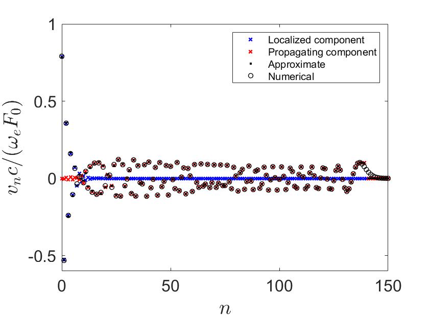
Figure 1: Comparison of the approximate solution (expression (14)) for the field of particle velocities at $\omega_{e}t=140$ and the driving frequency $\Omega=2.04\omega_{e}$ with the corresponding numerical solution. The red and blue crossed correspond to the contributions $v^{\omega}_{n,\mathrm{st}}$ and $v_{n}^{\Omega}$ respectively.

It is seen in Fig.1 that the approximate solution practically coincides with the results of numerical solution.

3.2.2 Case $0<\Omega<2\omega_{e}$

Before constructing the solution for this case, we note that the expression for the contribution $v^{\omega}_{n,\mathrm{cr}}$ for  $0\leqslant\Omega\leqslant 2\omega_{e}$ has a singularity. Introduce a real-valued coordinate $\tilde{n}_{g}$, at which the contribution is singular. From (13), we express the coordinate as

$$\tilde{n}_{g}=\omega_{e}t\sqrt{1-\frac{\Omega^{2}}{4\omega_{e}^{2}}}.$$ (15)

Note that the group velocity for the Hooke chain is determined as

$$v_{g}(\theta)\stackrel{{\scriptstyle\text{def}}}{{=}}a\frac{\mathrm{d}\omega}{\mathrm{d}\theta}=v_{s}\cos\frac{\theta}{2}\mathrm{sgn}\left(\sin\frac{\theta}{2}\right),$$ (16)

or, as the function of the dispersion relation:

$$v^{g}(\omega)=v_{s}\sqrt{1-\frac{\omega^{2}}{4\omega_{e}^{2}}}\mathrm{sgn}\,\omega.$$ (17)

Therefore, we can rewrite Eq.(15) as

$$\tilde{n}_{g}=\frac{v^{g}(\Omega)t}{a}.$$ (18)

For $0<\Omega<2\omega_{e}$, $\tilde{n}_{g}>0$ is the coordinate of a point, moving with the group velocity, corresponding to the frequency $\Omega$. We consider existence of the solution for the contributions to the field of particle velocity both behind the point $\tilde{n}_{g}$ and between $\tilde{n}_{g}$ and $\tilde{n}_{s}$. In the domain $\tilde{n}_{g}<n<\tilde{n}_{s}$, the solutions for $v^{\omega}_{n,\mathrm{cr}}$ and $v^{\Omega}_{n}$ cannot exist, because $\psi_{\tilde{n}_{g}<n<\tilde{n}_{s}}<\Omega$ for all time of motion of $\tilde{n}_{g}$ and thus wave with the frequency $\Omega$ cannot propagate. Based on aforesaid, we construct the following approximate solution for $v_{n}$:

$$v_{n}\approx v^{\omega}_{n,\mathrm{st}}+\left(v_{n}^{\Omega}+v^{\omega}_{n,\mathrm{cr}}\right)H(\tilde{n}_{g}-n),$$ (19)

where $v^{\omega}_{n,\mathrm{cr}}$ is determined by the expression (12). Thus, there is an additional wavefront, which propagates with the group velocity, corresponding to the frequency $\Omega$, besides one, propagating with the speed of sound. In contrast to the first term, which decays in time as $1/t^{\frac{3}{2}}$, the second term performs non-decaying oscillations with the frequency $\Omega$. Note that expression for the second term in (19) ($v_{n}^{\Omega}+v^{\omega}_{n,\mathrm{cr}}$) is the practically known result: the latter can be derived by differentiation with respect to time of Eq.(34) in [37]. In that work, the latter is understood as a solution of dynamical problem at large times. Here, we refine the latter by addition of the contribution $v^{\omega}_{n,\mathrm{st}}$ and by constraints on the existence of the term $v_{n}^{\Omega}+v^{\omega}_{n,\mathrm{cr}}$, which we calculate by using another method, based on the limiting absorption principle. Approximation of the field $v_{n}$ at the fixed moment of time is shown in Fig.2.

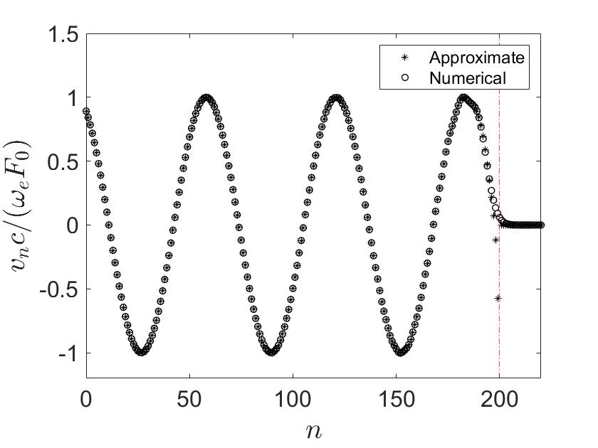
A

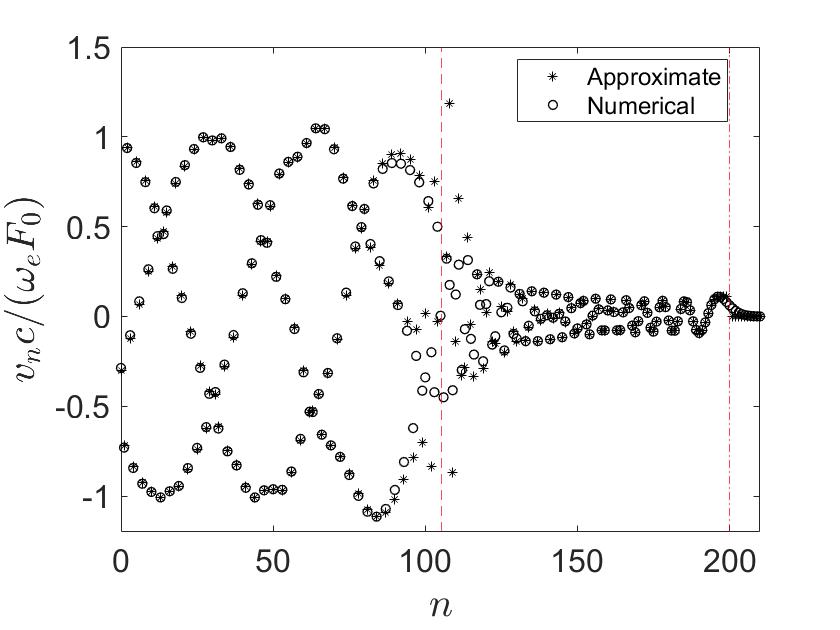
B

Figure 2: Comparison of the approximate solutions (expression (19)) for the field of particle velocities at $\omega_{e}t=200$ and for the driving frequencies $\Omega=0.1\omega_{e}$ (A) and $\Omega=1.7\omega_{e}$ (B) with the corresponding numerical solutions. The dashed and dash-dotted lines correspond to the coordinates of $\tilde{n}_{s}$ and $\tilde{n}_{g}$ respectively.

It is seen from Fig.2A that the velocity field is practically sinusoidal. Since the driving frequency is rather small ($\Omega\ll\omega_{e}$), the front $\tilde{n}_{g}$, carrying the energy, practically coincides with the front $\tilde{n}_{s}$, moving with the speed of sound. The effect of the dispersion can be negligible. For high driving frequencies, the case is quite another (see Fig.2B). The front $\tilde{n}_{g}$ moves significantly slower than $\tilde{n}_{s}$, what is shown below to affect the energy transfer into the chain. It is seen from Fig.2 that approximation for the velocity field, obtained here, becomes inadequate in the neighborhood of the wavefronts. The accurate estimation of the velocity field for $n\backsimeq\tilde{n}_{g}$ and $n=\tilde{n}_{s}$ is beyond the scope of present paper. If necessary, the latter can be performed by operation of the proposed in [53, 54] methods.

3.2.3 Case $\Omega=2\omega_{e}$

In this case,  $\tilde{n}_{g}=0$ and, therefore, the contribution $v_{n(\omega)}^{\mathrm{st}}$ is singular (and thus inaccurate) at the boundary. However, it is seen that the second expression in (12) becomes inaccurate for large enough $n$. Therefore, an approximate solution can be constructed by a crosslinking of the two solutions at a point $h$, which is not far from the free boundary:

$$v_{n}\approx v^{\omega}_{n,\mathrm{st}}H(n-h)+\left(v_{n}^{\Omega}+v^{\omega}_{n,\mathrm{cr}}\right)H(h-n).$$ (20)

Therefore, for $1\ll n<\tilde{n}_{s}$, the expression for particle velocity, $v_{n}$, can be written as

$$v_{n}\approx v^{\omega}_{n,\mathrm{st}}\approx\frac{F_{0}H(\tilde{n}_{s}-n)t}{\sqrt{\pi}m\sqrt[4]{\omega_{e}^{2}t^{2}-n^{2}}n}\sin\left(\psi_{n}t-\frac{\pi}{4}\right).$$ (21)

From Eq.(21) it is seen that, at $\Omega=2\omega_{e}$, expression for velocity of distant from the boundary particle grows in time as $\sqrt{t}$. Note that approximate solution for the field of particle velocity in the infinite Hooke chain (see time derivative of Eq.(1.58) in [52]) also grows in time as $\sqrt{t}$, however, with much larger amplitude than one in the semi-infinite Hooke chain because the latter decreases with increasing of $n$. Comparison of approximate and numerical solutions are shown in Fig.3. In particular, dependence of the $50$-th particle velocity is shown in Fig.3B.

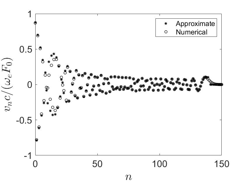
A

B

Figure 3: A: Comparison of the approximate solution (Eq.(20) at $h=10$) for the field of particle velocities at $\omega_{e}t=140$ and for the driving frequency $\Omega=2\omega_{e}$ with the corresponding numerical solution. B: Evolution in time of the $50$-th particle velocity at $\Omega=2\omega_{e}$.

It is seen in Fig.3 that approximate and numerical solutions are in good agreement except the neighborhood of the point $h$, in where the contributions, defined in the first and second terms in Eq.(20) are crosslinked. Comparing of the approximations (20) and (21) with time derivative of Eq.(25) in [37], we conclude that the latter result is erroneous.

Thus, at zero group velocity, the expression for the field of particle velocities grows in time. As it is shown below, the latter is reason of growth of the total energy, although the contributions from the oscillations with the driving frequency and from the singular point are also localized near the boundary (as at $\Omega>2\omega_{e}$).

In the next section, we estimate the total energy, supplied into the chain.

4 Energy transfer into the semi-infinite Hooke chain

4.1 Exact equation for the energy

According to the energy balance law, the total energy of the chain, $U$, is equal to the work, done by the external force to displace zeroth particle:

$$U=F_{0}\int_{0}^{t}v_{0}(\tau)\sin(\Omega\tau)\mathrm{d}\tau.$$ (22)

Substitution of $\eta=0$ and $n=0$ to (9) and then (9) to (22) using evenness property of the integrands yields

$$\begin{array}[]{l}\displaystyle U=\displaystyle\frac{2F_{0}^{2}\Omega}{m\pi v_{s}^{2}}\int_{0}^{\pi}\frac{v_{g}(\theta)^{2}\left(\Omega-\Omega\cos(\Omega t)\cos(\omega(\theta)t)-\omega\sin(\omega(\theta)t)\sin(\Omega t)\right)}{(\Omega^{2}-\omega(\theta)^{2})^{2}}\mathrm{d}\theta\\[8.53581pt] \displaystyle-\frac{F_{0}^{2}}{m\pi v_{s}^{2}}\int_{0}^{\pi}\frac{v_{g}(\theta)^{2}\sin^{2}(\Omega t)}{\Omega^{2}-\omega(\theta)^{2}}\mathrm{d}\theta.\end{array}$$ (23)

The equation (23) is the exact expression for the total energy of the semi-infinite chain. Below we investigate behavior of $U$ at large times.

4.2 Large time asymptotics

In order to estimate large time asymptotics for the total energy, we follow the proposed in [35] approach, simplifying expression for the energy (23). If the frequency $\Omega$ exceeds $2\omega_{e}$, i.e., does not belong the pass-band, defined by the dispersion relation, the total energy can not be permanently supplied into the chain for a reason discussed in Sect.3.2.1. The energy reaches some value and oscillates in time near it. Therefore, we consider only the case, when the driving frequency belongs to the pass-band ($\Omega\in(0;2\omega_{e}]$). At large time, the second term in (23) can be neglected by virtue of its boundedness, if the frequency $\Omega$ is not about zero.

Changing the wavenumber integral to the frequency integral in first term of (23), we rewrite expression for the energy $U$ as

$$\small U\approx\frac{2F_{0}^{2}\Omega a}{m\pi v_{s}^{2}}\int_{0}^{2\omega_{e}}\frac{v^{g}(\omega)\left(\Omega-\Omega\cos(\Omega t)\cos(\omega t)-\omega\sin(\omega t)\sin(\Omega t)\right)}{(\Omega^{2}-\omega^{2})^{2}}\mathrm{d}\omega,\normalsize$$ (24)

where $v^{g}$ is determined by Eq.(17). It is seen from expression (24) that the main contribution to the integral comes from vicinity of the point $\omega=\Omega$. Changing the variable in the integral in (24) $\epsilon=\Omega-\omega$ and, using the following asymptotic expansions with respect to $\epsilon/\omega_{e}$:

$$\begin{array}[]{l}\displaystyle\Omega-\Omega\cos(\Omega t)\cos(\omega t)-\omega\sin(\omega t)\sin(\Omega t)=2\Omega\sin^{2}\left(\frac{\epsilon t}{2}\right)+O\left(\frac{\epsilon}{\omega_{e}}\right),\\[5.69054pt] \displaystyle\Omega^{2}-\omega^{2}=2\Omega\epsilon+O\left(\left(\frac{\epsilon}{\omega_{e}}\right)^{2}\right),\\[5.69054pt] \displaystyle v^{g}(\omega)=v^{g}(\Omega)+O\left(\frac{\epsilon}{\omega_{e}}\right),\end{array}$$ (25)

we rewrite the expression for the total energy as

$$U\approx\frac{F_{0}^{2}av^{g}(\Omega)}{m\pi v_{s}^{2}}\int_{\Omega-2\omega_{e}}^{\Omega}\frac{\sin^{2}\left(\frac{\epsilon t}{2}\right)}{\epsilon^{2}}\mathrm{d}\epsilon.$$ (26)

Tending in the integral in (26) $\epsilon t\rightarrow\infty$ and using the identity

$$\int_{0}^{\infty}\frac{\sin^{2}\frac{x}{2}}{x^{2}}\mathrm{d}x=\frac{\pi}{4},$$ (27)

we write expression for energy, supplied into the chain at large times, in the final form:

$$U\approx\frac{F_{0}^{2}v^{g}(\Omega)at}{2mv_{s}^{2}}.$$ (28)

According to (28), the total energy, supplied into the chain by periodic force loading, linearly grows in time. The reason of the growth is propagation of the non-decaying oscillations through the chain with the group velocity (see Sect.3.2.2 for details). The more frequency $\Omega$ is the slower front $\tilde{n}_{g}$, carrying the energy, propagates and thus the rate of energy supply is less. For the first time the result was obtained in [37] in terms of the average power supply (i.e., $\dot{U}$).

Note that the total energy, supplied into the infinite Hooke chain and is expressed as (see expression (18) in [35])

$$U_{\mathrm{inf}}\approx\frac{F_{0}^{2}at}{4mv^{g}(\Omega)},$$ (29)

grows also linearly in time but is inversely proportional to the group velocity, owing to which rate of energy grows with increasing of $\Omega$.

In order to check the expression (28), we perform numerical integration of Eqs. (4) in the same way as discussed in Sect.3.2. The obtained particle velocities and displacements are used for calculation the total energy of the chain. Comparison of the expressions (28) with the numerical solution and (29) is shown in Fig.4.

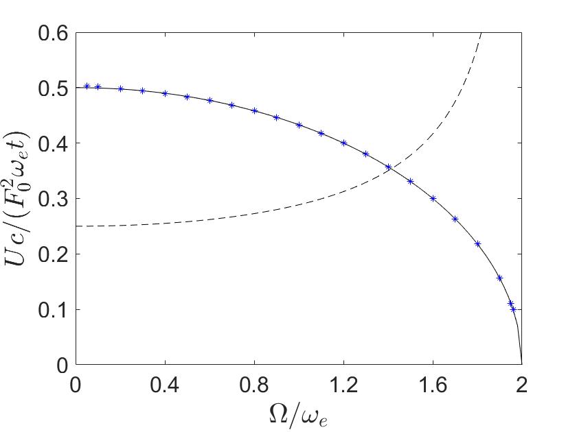
Figure 4: Dependence of rate of growth of the total energy, supplied into the semi-infinite ((28), solid line) and infinite ((29), dashed line) chains versus the excitation frequency $\Omega$. Results of the numerical simulations are shown by the asterisks.

It is seen that energy is supplied into the semi-infinite chain faster than into the infinite chain at the driving frequencies $\Omega\in\left(0;\sqrt{2}\omega_{e}\right)$. At the driving frequencies $\Omega\in\left(\sqrt{2}\omega_{e};2\omega_{e}\right)$ energy is supplied to the infinite chain faster than to the semi-infinite chain. Note that, at low frequencies, the energy supplied into the semi-infinite chain is approximately 2 times more than the one supplied into the infinite chain. Therefore, for $\Omega\ll\omega_{e}$, the problem on energy supply may be considered symmetric with respect to zero particle. Note also that energy supply into the infinite elastic bar (model of the Hooke chain in the continuum limit), caused by the force loading, is estimated in [35] (see expression (50) therein). The expression for the energy, transmitted to the infinite bar has the same form as for the infinite Hooke chain, if $v^{g}$ in (29) is replaced by $v_{s}$. The latter is satisfied also for the semi-infinite elastic bar (according to the comparison of (28) and the expression (49) in [35]). Therefore, energy transfer into the semi-infinite Hooke chain can be estimated by the continuum model only for low driving frequencies. It is also seen that asymptotic solution for the energy in the semi-infinite chain is estimated with high accuracy.

At the cut-off frequency, $\Omega=2\omega_{e}$ (at zero group velocity), the asymptotic approximation (28) becomes inapplicable. In this case, we derive the latter as follows. Rewrite the asymptotic expansions (25) with respect to $\epsilon=2\omega_{e}-\omega$ as

$$\begin{array}[]{l}\displaystyle\Omega-\Omega\cos(\Omega t)\cos(\omega t)-\omega\sin(\omega t)\sin(\Omega t)=4\omega_{e}\sin^{2}\left(\frac{\epsilon t}{2}\right)+O\left(\frac{\epsilon}{\omega_{e}}\right),\\[5.69054pt] \displaystyle\Omega^{2}-\omega^{2}=4\omega_{e}\epsilon+O\left(\left(\frac{\epsilon}{\omega_{e}}\right)^{2}\right),\\[5.69054pt] \displaystyle v_{g}\approx v_{s}\sqrt{\displaystyle\frac{\epsilon}{\omega_{e}}}+O\left(\left(\frac{\epsilon}{\omega_{e}}\right)^{\frac{3}{2}}\right).\end{array}$$ (30)

Therefore, expression for the energy can be approximately rewritten in the form

$$U\approx\frac{F_{0}^{2}a\sqrt{t}}{\pi mv_{s}\sqrt{\omega_{e}}}\int_{0}^{2\omega_{e}t}\frac{\sin^{2}\left(\frac{\epsilon t}{2}\right)}{(\epsilon t)^{\frac{3}{2}}}\mathrm{d}(\epsilon t).$$ (31)

Tending in (31) $\epsilon t\rightarrow\infty$ and using the identity

$$\int_{0}^{\infty}\frac{\sin^{2}\frac{x}{2}}{x^{\frac{3}{2}}}\mathrm{d}x=\sqrt{\frac{\pi}{2}},$$ (32)

we write expression for energy, supplied into the chain at large times, in the final form:

$$U\approx\frac{F_{0}^{2}\sqrt{t}}{m\sqrt{2\pi\omega_{e}^{3}}}.$$ (33)

Therefore, at the frequency $\Omega=2\omega_{e}$ energy grows in time proportionally to $\sqrt{t}$. In this case, the reason of the growth is increasing in time of the field of particle velocities (and, therefore, field of particle displacements). Note that energy, supplied into the infinite chain at the same frequency, grows in time as $t^{3/2}$ (see expression (19) in [35]) and the growth is caused by the same [52]. The reason of different asymptotic behavior of the total energy of the infinite and semi-infinite chains may be caused by peculiarities of growth of amplitudes of the corresponding fields of particle velocity. A comparison of the expression (33) with the numerical results is discussed in Sect.5.2.

Thus, analytical estimation of the energy transfer into the semi-infinite Hooke chain is performed. We show in the next section that the expression (28) serves for zeroth approximation for the solution in the anharmonic case.

5 Energy transfer into the $\beta$-FPUT chain

In the section, we investigate manifestation of anharmonicity on the behavior of energy, supplied into the semi-infinite chain and perform large-time asymptotic estimation for it. The total energy can be calculated via Eq.(22) by substitution of asymptotic expansion for the velocity of zeroth particle up to order of $\beta F_{0}^{2}/c^{3}$, which can be obtained by means of the perturbation analysis (see, e.g., [56, 57]). However, this approach involves technical difficulties and, therefore, we propose the following strategy below.

5.1 Quasiharmonic approximation for the energy

We refer to the wave turbulence theory (see, e.g., [58]). According to it, the main contribution to the energy exchange between waves, induced by the cubic nonlinearity, comes from the four-wave trivial resonant (2 $\rightarrow$ 2)-type interactions. The dispersion relation, corresponding to the harmonic part of the Hamiltonian is the renormalized dispersion relation. For the $\beta$-FPUT chain, the latter is analyzed in papers [60, 61, 62]. In order to estimate the total energy, we make use of expression for the renormalized dispersion relation, obtained in the paper [60] (see Eq.(3) therein).

Remark 1. The expression for the renormalized dispersion relation of $\beta$-FPUT chain may also be derived in the different ways, for instance, as discussed in [61]. Comparison of these ways with one, considered here, is beyond the scope of present paper.
For the semi-infinite chain, we rewrite equation for the latter as

$$\tilde{\omega}=\lambda\omega,\quad\lambda=\sqrt{1+\frac{3\beta}{2\pi c\omega_{e}^{2}}\int_{-\pi}^{\pi}\langle\hat{u}(t)^{2}\rangle_{t}\omega(\theta)^{2}\mathrm{d}\theta}.$$ (34)

where $\lambda$ is the renormalized factor; $\hat{u}$ is the direct DCT of the particle displacement, which, in general case (for arbitrary $\beta$), is unknown; the $\langle...\rangle_{t}$ stands for the time averaging. Here, we average over period of the weakly anharmonic Duffing oscillator:

$$\langle...\rangle_{t}=\frac{1}{\tau_{D}}\int_{0}^{\tau_{D}}...\mathrm{d}t,\quad\tau_{D}=\frac{2\pi}{\omega_{e}}\left(1-\frac{3\beta F_{0}^{2}}{8c^{3}}\right)+O\left(\frac{\beta^{2}F_{0}^{4}}{c^{6}}\right).$$ (35)

Remark 2. The renormalized dispersion relation is derived in [60] under assumption that the $\beta$-FPUT chain is strongly nonlinear and is in thermal equilibrium. This is not our case. Here, $\tilde{\omega}$ is understood as some equivalent linear dispersion relation, which is analogous to the equivalent linear frequency, in terms of which some dynamical problems of nonlinear oscillators may be solved (see, e.g., [64, 65]).
Note that, firstly, the renormalized factor does not depend on the wavenumber $\theta$. Secondly, since we calculate $\lambda$ with accuracy up to order of $\beta F_{0}^{2}/c^{3}$, the expression for $\hat{u}$ in the harmonic approximation can be used. Substitution of (8) at $\eta=0$ and (35) to (34) and further simplification with remaining terms of order of $\beta F_{0}^{2}/c^{3}$, yields the following approximation for $\lambda$:

$$\begin{array}[]{l}\lambda\approx 1\displaystyle+\frac{\beta F_{0}^{2}}{c^{3}}\mu(\Omega),\\[8.53581pt] \mu(\Omega)=\displaystyle\frac{3\omega_{e}^{2}}{8\pi^{2}}\int_{0}^{2\pi}\int_{0}^{2\pi}\frac{\cos^{2}\frac{\theta}{2}\Bigl{(}\Omega\sin(\omega(\theta)t)-\omega(\theta)\sin(\Omega t)\Bigr{)}^{2}}{(\Omega^{2}-\omega(\theta)^{2})^{2}}\mathrm{d}({\omega_{e}t})\mathrm{d}\theta.\end{array}$$ (36)

In simulations, the integral in (36) is calculated using the rectangular rule with division of the integration domain on $10^{6}$ equal squares. Dependence of the function $\mu$, determining the renormalization factor, on the excitation frequency is shown in Fig.5.

Figure 5: Dependence of the function $\mu$ on the frequency $\Omega$.

For convenience, we rewrite $\mu$ in the following approximate form, which is satisfied for $\Omega/\omega_{e}\in[1.5;2.1]$:

$$\mu\approx 0.848\left(\frac{\Omega}{\omega_{e}}\right)^{3}-4.580\left(\frac{\Omega}{\omega_{e}}\right)^{2}+7.591\left(\frac{\Omega}{\omega_{e}}\right)-3.332.$$ (37)

We assume that the main contribution to energy transmission comes from the oscillations with frequencies, which belong to the renormalized dispersion relation $\tilde{\omega}$ and from the harmonic oscillations with the driving frequency $\Omega$ (subharmonic (with the frequencies $m$ times less $\Omega$ ($\kappa\in\mathbb{N},\kappa>1$), see, e.g., [66] for details) and superharmonic (with the frequencies $m$ times more $\Omega$ ($\kappa\in\mathbb{N},\kappa>1$)) oscillations are neglected). Then, taking into account the first equation in Eq. (34) and (36) and supposing that $\Omega$ is not too close to zero, we rewrite Eq.(24) for the energy, transmitted into the chain, with respect to $\tilde{\omega}$, namely

$$U\approx\frac{2F_{0}^{2}\Omega a}{m\lambda\pi v_{s}^{2}}\int_{0}^{\tilde{\omega}_{\max}}\frac{v^{g}\left(\frac{\tilde{\omega}}{\lambda}\right)\left(\Omega-\Omega\cos(\Omega t)\cos(\tilde{\omega}t)-\tilde{\omega}\sin(\tilde{\omega}t)\sin(\Omega t)\right)}{(\Omega^{2}-\tilde{\omega}^{2})^{2}}\mathrm{d}\tilde{\omega},$$ (38)

where $\tilde{\omega}_{\max}$ is the maximal value of the renormalized dispersion relation. Performing the same operations as done in Sect.4.2 yields the following asymptotic approximation for the total energy:

$$U\approx\displaystyle\frac{F_{0}^{2}v^{g}\left(\displaystyle\frac{\Omega}{\lambda}\right)at}{2m\lambda v_{s}^{2}}.$$ (39)

Substituting (36) to (39) and preserving the terms of order of $\beta F_{0}^{2}/c^{3}$, we obtain the final expression for the total energy

$$U\approx\displaystyle\frac{F_{0}^{2}v^{g}\left(\tilde{\Omega}\right)at}{2mv_{s}^{2}}\left(1-\frac{\beta F_{0}^{2}}{c^{3}}\mu\right),\quad\tilde{\Omega}=\Omega\left(1-\frac{\beta F_{0}^{2}}{c^{3}}\mu\right).$$ (40)

Therefore, expression for the total energy, supplied into the chain, is represented as a sum of harmonic approximation at the frequency $\tilde{\Omega}$ and correction, directly proportional to the first term. Further, we refer (40) to as a quasiharmonic approximation. It is seen from (40) that, firstly, as expected, energy dependence on $F_{0}^{2}$ is not linear. Secondly, the expression (40) is valid not only for the cutoff frequency of the Hooke chain ($\Omega=2\omega_{e}$) but for frequencies, which may slightly exceed this value. From (40), we determine a maximal frequency, permitting passing waves into the chain, $\Omega_{\mathrm{cr}}$, satisfies the equation

$$\Omega_{\mathrm{cr}}\left(1-\frac{\beta F_{0}^{2}}{c^{3}}\mu(\Omega_{\mathrm{cr}})\right)=2\omega_{e}.$$ (41)

The value of $\Omega_{\mathrm{cr}}$ is found from Eq.(41) with accuracy up to order of $\beta F_{0}^{2}/c^{3}$ as (see Appendix D):

$$\Omega_{\mathrm{cr}}\approx\left(2+2\mu(2\omega_{e})\frac{\beta F_{0}^{2}}{c^{3}}\right)\omega_{e}.$$ (42)

From (37), $\mu(2\omega_{e})\approx 0.314$. In order to check accuracy of the approximations (40) and (42), we perform the numerical simulations by integration of Eqs.(1) in the same way as described in Sect.3.2. The obtained particle velocities and displacements are used for calculation the total energy of the chain. Further, we investigate evolution of the total energy at large times and for different types of the driving frequencies.

5.2 Energy propagation at frequencies, lying in the pass-band of the Hooke chain

Evolution of the total energy at large times and at $\Omega\in(0;2\omega_{e})$ for $\beta F_{0}^{2}/c^{3}=0.1$ is shown in Fig.6A.

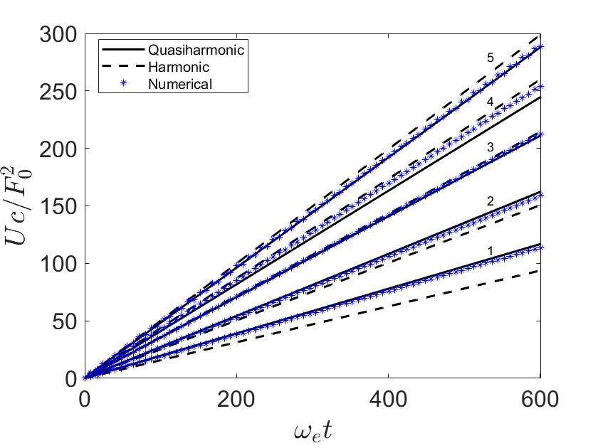
A

B

Figure 6: A: Asymptotic solutions for the total energy, supplied into the semi-infinite chain for $\beta F_{0}^{2}/c^{3}=0.1$ at frequencies $\Omega=1.90\omega_{e}$ (1), $\Omega=1.73\omega_{e}$ (2), $\Omega=1.41\omega_{e}$ (3), $\Omega=\omega_{e}$ (4), $\Omega=0.20\omega_{e}$ (5) in the harmonic and quasiharmonic approximations (expressions (28) and (40) respectively). B: Relative error of asymptotic solution for the rate of energy supply into the harmonic (dashed line) and quasiharmonic (solid line) approximations for $\beta F_{0}^{2}/c^{3}=0.02$ (red line) and $\beta F_{0}^{2}/c^{3}=0.1$ (black line).

It is seen that asymptotics for the energy in the harmonic approximation (28) is valid at short times for all range of the considered driving frequencies. For the frequency $\Omega=1.41\omega_{e}$, results, obtained in harmonic approximation, coincide with results, obtained in the quasiharmonic approximation (dashed and solid lines coincide, see Fig.6A), and also with the results of numerical simulations. However, at large times, manifestation of nonlinearity occurs. For instance, for the frequencies $\Omega=1.90\omega_{e}$, $\Omega=1.73\omega_{e}$ and $\Omega=0.20\omega_{e}$ description of the energy supply is more accurate in quasiharmonic approximation than in the harmonic one. Wherein, however, for $\Omega=\omega_{e}$, the harmonic approximation is more correct than the quasiharmonic one. In order to analyze accuracy of the asymptotic approximations in detail, we calculate the relative error between $\dot{U}_{\mathrm{asympt}}$ (using the expressions (28) and (40) for the harmonic and quasiharmonic approximations respectively) and $\dot{U}_{\mathrm{num}}$, averaged over time interval, equal to $10^{3}/\omega_{e}$, for range of the frequencies $\Omega\in[0.09\omega_{e};1.95\omega_{e}]$. One can see in Fig.6B that, for the driving frequencies, which are close to the cut-off frequency of the Hooke chain, the relative error of the harmonic approximation is sufficiently higher than one of the quasiharmonic approximation. Therefore, for the driving frequency $\Omega\lessapprox 1.5\omega_{e}$, energy transfer can be estimated in the harmonic approximation with reasonable accuracy.

Consider evolution of the total energy, transferred into the chain at the cut-off frequency of the Hooke chain. Time dependence of the total energy is shown in Fig.7.

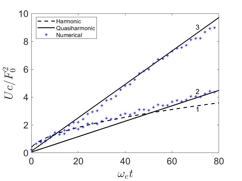
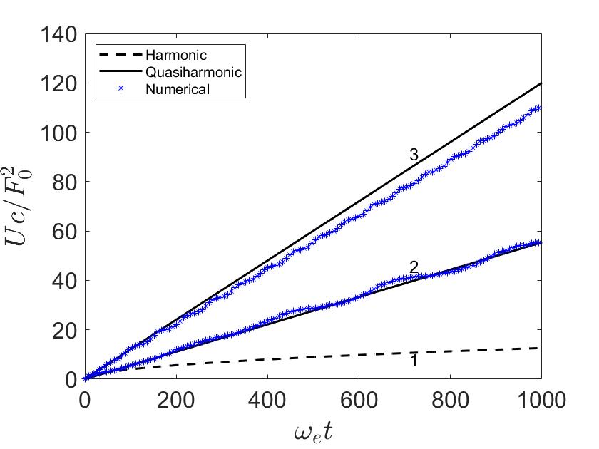
Figure 7: Evolution of energy, supplied into the semi-infinite chain at the cut-off frequency of the harmonic chain ($\Omega=2\omega_{e}$) at short times (left) and at large times (right). Asymptotic solution is shown for $\beta F_{0}^{2}/c^{3}=0$ (1, expression (33)), $\beta F_{0}^{2}/c^{3}=0.02$ (2, expression (40)), $\beta F_{0}^{2}/c^{3}=0.1$ (3, expression (40)).

It is seen in Fig.7 that energy supply at $\Omega=2\omega_{e}$ has two time scales. The first time scale corresponds to growth of the total energy, which can be adequately described in the harmonic approximationexpression (expression (33)). Starting from some time, the rate of propagation undergoes sharp increase. Evolution of the energy may be then described in the quasiharmonic approximation with rather high accuracy (at least at times $\omega_{e}t<250$, see Fig.7 (right)).

5.3 Energy propagation at frequencies, lying in the stop-band of the Hooke chain

We consider energy supply into the semi-infinite chain at $\Omega>2\omega_{e}$. The loading with the frequency, exceeding $2\omega_{e}$, results in energy supply into the chain (see Fig.8).

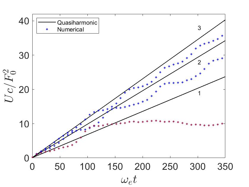
Figure 8: Asymptotic approximation (40) for energy, supplied into the semi-infinite chain at the frequencies $\Omega=2.005\omega_{e}$ (3), $\Omega=2.02\omega_{e}$ (2), $\Omega=2.04\omega_{e}$ (1). Comparison of the asymptotic and numerical solutions is shown for $\beta F_{0}^{2}/c^{3}=0.1$.

In order to understand nature of sharp increase of the supplied energy, we perform set of numerical experiments (See Sect.5.1 for details). These experiments revealed a localized mode, which moves slower than the decaying perturbations moving with the speed of sound. Moreover, a numerical experiment, performed for the free semi-infinite Hooked chain ($\beta=0,F=0$) showed that the launched same localized mode is extinguished. According to the aforesaid observations, we suppose that the reason of the energy supply is the supratransmission and the source of the transferred into the chain energy (as well as for $\Omega=2\omega_{e}$) is, apparently, intrinsic localized modes. It is seen in Fig.8 that, firstly, evolution of the total energy can be well-described in the quasiharmonic approximation (39) at least at times $\omega_{e}t<150$. However, the quasiharmonic approximation becomes hereafter no longer valid owing to the either slowdown or stop of this process, therefore, at high driving frequencies and sufficiently large times, energy does not grow linearly. Apparently, corrections of order of $\beta^{2}F_{0}^{4}/c^{6}$ are required for more accurate description of this process. Secondly, one can see that small change of the driving frequency results in sufficient change of rate of the transfer.

Consider the case when the excitation frequency is close to $\Omega_{\mathrm{cr}}$. We calculate numerically the total energy of the chain for frequencies $2\omega_{e}\leqslant\Omega\leqslant\Omega_{\mathrm{cr}}$ and $0<\beta F_{0}^{2}/c^{3}\leqslant 0.1$ and then compare results with the quasiharmonic approximation (40). The ratios between $\Omega/\omega_{e}$ and $\beta F_{0}^{2}/c^{3}$, corresponding to the different situations, concerning energy transmission into the chain, are shown in Fig.9. There are such ratios, at which the energy is not transmitted into the chain, according to the both simulations and the quasiharmonic approximation (40). These ratios are marked in the diagram, shown in Fig.9 by the triangles above the dividing line, determining $\Omega_{\mathrm{cr}}$ by means of the prediction (42).

Figure 9: Diagram of ratios between anharmonic force $\beta F_{0}^{2}/c^{3}$ and $\Omega/\omega_{e}$, corresponding to different character of the energy supply. The quasiharmonic approximation ((42), solid line) and numerical results (triangles, circles and squares).

There are such values of $\Omega/\omega_{e}$ and $\beta F_{0}^{2}/c^{3}$, at which energy is transmitted into the chain and the quasiharmonic approximation is in agreement with it (marked by the squares). However, according to the numerical results, several values of $\Omega/\omega_{e}$ and $\beta F_{0}^{2}/c^{3}$ correspond to inability to pass energy into the chain, while the quasiharmonic approximation (42) shows in the contrary. These values are marked by the circles and are redistributed between the triangles and squares. Therefore, the real value of the frequency, permitting energy transmission, is less than $\Omega_{\mathrm{cr}}$. Apparently, neglecting non-trivial resonant or ($3\rightarrow 1$)- and ($4\rightarrow 0$)-type interactions in the assessment of the total energy might result in some error in (38) and (42). We do not consider the question in detail in the current work.

The expression (42) may be estimated as an upper boundary of the critical frequency. A lower boundary of the critical frequencies can be contingently determined by straight line to the point $(0.10;2.045)$. The slope of the latter ($0.450$) is less than one, corresponding to the upper boundary ($2\mu(2\omega_{e})\approx 0.628$).

Remark 3. We have reproduced the numerical calculations of the total energy, having replaced $\sin(\Omega t)$ in right part of Eq.(1) by $\cos(\Omega t)$ and have convinced that this action does practically not affect on the obtained in this section (and in the present paper at whole) results.

6 Conclusions

Energy supply into the semi-infinite $\beta$-FPUT chain by the sudden periodic force loading was considered. In this case, the loading results in growth of the supplied energy. Asymptotic peculiarities of the growth at large times have been estimated.

A modification of the Hemmer approach, which allows to obtain an approximate solution of a dynamical problem in the harmonic approximation (namely, for the Hooke chain) is proposed (Sect.3.2). Herewith, the contribution, corresponding tho the forced oscillations, is found exactly while for the second contribution, corresponding tho the natural oscillations, the large-time asymptotic estimation is performed. Obtained expressions for the contributions are used to construct the approximate solution, which is refined version of the dynamical problem solution got in [37] and upon which the explanation of mechanism of energy supply into the chain at large time is based. At low driving frequencies an effect of free boundary may be shown to be neglected: a process of energy supply is qualitatively indistinguishable from the same process both in the infinite chain and in the elastic rod (see [35]). However, at high frequencies, rate of energy supply decreases with increasing of the driving frequency (in contrast to the infinite chain).

In the weakly anharmonic case, the process of energy supply can be described in the harmonic approximation for short times at driving frequencies, lying in the pass-band of the Hooke chain. At large times, the harmonic approximation is reasonably accurate for $\Omega\lessapprox 1.5\omega_{e}$. For general case, asymptotic solution for the total energy (referred further to as the quasiharmonic approximation) was obtained (expression (40)) by dint of the derived in [60] and rewritten for the semi-infinite chain equation for the renormalized dispersion relation. It was shown that the quasiharmonic approximation is suitable for description of energy transfer at large times (of order at least of $150/\omega_{e}$) under force loading with the driving frequency, which both may be equal to $2\omega_{e}$ and may lie in the stop band of the Hooke chain. By using the first term in (40), approximation for the frequency, above which the energy transmission into the chain is impossible ($\Omega_{\mathrm{cr}}$), was obtained (expression (42)). However, the results of numerical analysis have shown that the real value of this frequency is less than $\Omega_{\mathrm{cr}}$ for any power of anharmonicity.

The results of the current work can be generalized into the cases of the interactions via more physically realistic (than $\beta$-FPUT) potentials. Consideration of the cases of loading by a force, arbitrary changing in time, will be also an interesting extension of the present paper. Results with regard to energy transport in this case may serve for development of theory of heat transport at the nanoscale in the frameworks of the lattice dynamics approach. In particular, a problem on propagation of thermal wave through the interface between two dissimilar semi-infinite homogeneous chains can be interpreted in terms of dynamics of the one chain segment, undergone an equivalent force, acting from the second segment. An expression for this force is unknown. However, by using the approaches based on the energy dynamics [44], one can obtain some quantities without calculation of the equivalent force itself (see [67]). The results, concerning asymptotic assesses of the supplied total energy are expected to serve for simplification of aforesaid problem, concerning inhomogeneous anharmonic lattices. Understanding of the heat transport therein is important for development of thermal diode techniques (see, e.g., [68, 69, 70, 71]), because making up the thermal diode lattices are nonlinear.

Conflict of interest

None to declare.

Appendix A Derivation of Eq. (10)

Here, we derive Eq. for the contribution $v_{n(\Omega)}$ in the closed form. Using the following approximations due to $\eta/\omega_{e}$ is infinitesimal:

$$\begin{array}[]{l}\displaystyle\phi_{2}\approx\pi,\\[8.53581pt] \displaystyle\sqrt{\Omega^{2}-\omega^{2}\pm 2\mathrm{i}\eta\Omega}\approx\sqrt{\Omega^{2}-\omega^{2}}\pm\frac{\mathrm{i}\eta\Omega}{\sqrt{\Omega^{2}-\omega^{2}}},\end{array}$$ (43)

rewrite the expression for $v_{n(\Omega)}$ in Eq.(9) as follows:

$$v_{n(\Omega)}\approx-\frac{F_{0}\Omega\cos(\Omega t)H(t)}{m}\left(\mathrm{I}_{n}+\mathrm{I}_{n+1}+\mathrm{c.c.}\right),\quad\mathrm{I}_{n}=\frac{1}{4\pi}\int_{-\pi}^{\pi}\frac{e^{\mathrm{i}n\theta}\mathrm{d}\theta}{\Omega^{2}-\omega^{2}-\mathrm{i}\eta\Omega},$$ (44)

where $\mathrm{c.c.}$ stands for the complex conjugate terms. We transform the integral in Eq.(44) to the unit circle integral. Put $z=e^{\mathrm{i}\theta}$. Then

$$\mathrm{d}\theta=-\mathrm{i}\frac{\mathrm{d}z}{z},\qquad 2\cos\theta=z+\frac{1}{z},$$ (45)

and, therefore,

$$\mathrm{I}_{n}=-\frac{\mathrm{i}}{4\pi}\int_{|z|=1}\frac{z^{n}\mathrm{d}z}{\omega_{e}^{2}z^{2}+(\Omega^{2}-2\omega_{e}^{2}-\mathrm{i}\eta\Omega)z+\omega_{e}^{2}}.$$ (46)

Rewrite Eq.(46) as

$$\begin{array}[]{l}\displaystyle\mathrm{I}_{n}=-\frac{\mathrm{i}}{4\pi\omega_{e}^{2}(z_{1}-z_{2})}\left(\int_{|z|=1}\frac{z^{n}\mathrm{d}z}{z-z_{1}}-\int_{|z|=1}\frac{z^{n}\mathrm{d}z}{z-z_{2}}\right),\\[14.22636pt] \displaystyle z_{1,2}=\frac{2\omega_{e}^{2}-\Omega^{2}+\mathrm{i}\eta\Omega\pm\mathrm{i}\sqrt{\Omega}\sqrt{\Omega-\mathrm{i}\eta}\sqrt{4\omega_{e}^{2}-\Omega^{2}+\mathrm{i}\eta\Omega}}{2\omega_{e}^{2}}.\end{array}$$ (47)

where $z_{1}$ and $z_{2}$ are roots of the denominator of the integrand in Eq.(46), i.e., poles. Rewrite the latter in the limit $\eta\rightarrow 0+$:

$$z_{1,2}=1-\frac{\Omega^{2}}{2\omega_{e}^{2}}\pm\mathrm{i}\left(\frac{\Omega\sqrt{4\omega_{e}^{2}-\Omega^{2}}}{2\omega_{e}^{2}}+0\right).$$ (48)

Consider $0<\Omega<2\omega_{e}$. In this case, the pole $z_{2}$ lies inside the unit circle $|z|<1$ only. Therefore, we take into account the residue at $z_{2}$ only and the first term in (47) equals zero. Therefore, we have

$$\mathrm{I}_{n}=\frac{\mathrm{i}z_{2}^{n}}{2\Omega\sqrt{4\omega_{e}^{2}-\Omega^{2}}}=\frac{(-1)^{n}e^{2\mathrm{i}\varphi n}}{-2\mathrm{i}\Omega\sqrt{4\omega_{e}^{2}-\Omega^{2}}},\quad\varphi=\arccos{\frac{\Omega}{2\omega_{e}}}.$$ (49)

Consider $\Omega>2\omega_{e}$. In this case, Eqs. for $z_{1,2}$ have the form

$$z_{1,2}=1-\frac{\Omega^{2}\pm\Omega\sqrt{\Omega^{2}-4\omega_{e}^{2}}}{2\omega_{e}^{2}}.$$ (50)

Substituting $z_{1,2}$ to Eq.(47) with taking into account $|z_{2}|<1$ yields

$$\begin{array}[]{l}\displaystyle\mathrm{I}_{n}=\frac{z_{2}^{n}}{2\Omega\sqrt{\Omega^{2}-4\omega_{e}^{2}}}=\frac{(-1)^{n}e^{-\gamma n}}{2\Omega\sqrt{\Omega^{2}-4\omega_{e}^{2}}},\\[5.69054pt] \displaystyle\gamma=-\ln\left(\frac{\Omega^{2}-\Omega\sqrt{\Omega^{2}-4\omega_{e}^{2}}}{2\omega_{e}^{2}}-1\right)=2\mathrm{arccosh}\frac{\Omega}{2\omega_{e}}.\end{array}$$ (51)

Consider $\Omega=2\omega_{e}$. The integral for $\mathrm{I}_{n}$ and its complex conjugation, $\bar{\mathrm{I}}_{n}$, determined in (44), can be analogously transformed into the unit circle integral and then to the form

$$\begin{array}[]{l}\displaystyle\mathrm{I}_{n}=-\frac{\mathrm{i}}{4\pi\omega_{e}^{2}}\int_{|z|=1}\frac{z^{n}\mathrm{d}z}{(z+1-\mathrm{i}0)^{2}}=0,\\[5.69054pt] \displaystyle\bar{\mathrm{I}}_{n}=-\frac{\mathrm{i}}{4\pi\omega_{e}^{2}}\int_{|z|=1}\frac{z^{-n}\mathrm{d}z}{(z+1+\mathrm{i}0)^{2}}=\frac{(-1)^{(n+1)}n}{2\omega_{e}^{2}}.\end{array}$$ (52)

Here, the following identities [72]

$$\frac{1}{(z\pm\mathrm{i}0)^{2}}=\pm\mathrm{i}\pi\delta^{\prime}(z)+\mathrm{p.v.}\frac{1}{z^{2}},$$ (53)

where $\mathrm{p.v.}$ stands for the Cauchy principle value, are used. Substitution of Eqs. (49), (51), (52) to Eq.(44) with respect to the corresponding values of the driving frequency and with further simplifications yields Eq.(10). Note that the expressions (49), (51), (52) were previously obtained in [52]. However, Eqs. (49)+$\mathrm{c.c.}$ and (52) were obtained in the sense of the Cauchy principal value only, while, here, we do this exactly by using the limiting absorption principle.

Appendix B Derivation of expression (12)

Rewrite Eq. for $v_{n(\omega)}$ in Eq.(9) as follows:

$$v_{n(\omega)}=\frac{2F_{0}\Omega e^{-\eta t}H(t)}{m\pi}\int_{0}^{\pi}\frac{(\Omega^{2}-\omega(\theta)^{2})\cos(\omega(\theta)t)}{(\Omega^{2}-\omega(\theta)^{2})^{2}+4\eta^{2}\Omega^{2}}\cos\frac{(2n+1)\theta}{2}\cos\frac{\theta}{2}\mathrm{d}\theta.$$ (54)

Here, we use the following approximations due to $\eta/\omega_{e}$ is infinitesimal:

$$\begin{array}[]{l}\displaystyle\phi_{1}\approx\left[\begin{gathered}0,\,\omega<\Omega;\\ \pi,\,\omega>\Omega,\\ \end{gathered}\right.\\[14.22636pt] \sqrt{\omega^{2}-\eta^{2}}\approx\omega,\quad\sqrt{4\eta^{2}(\omega^{2}-\eta^{2})+(\Omega^{2}-\omega^{2}+2\eta^{2})^{2}}\approx|\Omega^{2}-\omega^{2}|.\end{array}$$ (55)

Rewrite the wavenumber integral (54), changing to the frequency integral:

$$\begin{array}[]{l}\displaystyle v_{n(\omega)}=\frac{2F_{0}\Omega e^{-\eta t}H(t)}{m\omega_{e}\pi}\int_{0}^{2\omega_{e}}\frac{(\Omega^{2}-\omega^{2})\cos(\omega(\theta)t)}{(\Omega^{2}-\omega^{2})^{2}+4\eta^{2}\Omega^{2}}\cos\left((2n+1)\arcsin\frac{\omega}{2\omega_{e}}\right)\mathrm{d}\omega.\end{array}{}$$ (56)

Introduce a function, $\mathrm{I}_{n}^{\mathrm{cr}}$, which denotes the contribution to Eq.(54), coming from the vicinity of the point $\Omega=\omega$. We introduce a variable $\epsilon=\Omega-\omega$, which is infinitesimal for infinitesimal value $\eta/\omega_{e}$. Consider two cases: $0<\Omega<2\omega_{e}$ and $\Omega=2\omega_{e}$. In the first case we transform (54), using the following asymptotic expansions with respect to $\epsilon/\omega_{e}$:

$$\begin{array}[]{l}\displaystyle\Omega^{2}-\omega^{2}=2\Omega\epsilon+O\left(\left(\frac{\epsilon}{\omega_{e}}\right)^{2}\right),\\[5.69054pt] \displaystyle\cos\left((2n+1)\arcsin\frac{\omega}{2\omega_{e}}\right)=\cos\left((2n+1)\arcsin\frac{\Omega}{2\omega_{e}}\right)+O\left(\frac{\epsilon}{\omega_{e}}\right).\end{array}$$ (57)

Based on aforesaid, we write equation for $\mathrm{I}^{\mathrm{cr}}_{n}$ as the integral along the vicinity of $\epsilon=0$:

$$\begin{array}[]{l}\displaystyle\mathrm{I}^{\mathrm{cr}}_{n}=\frac{F_{0}e^{-\eta t}H(t)\mathcal{T}_{2n+1}\left(\sqrt{1-\frac{\Omega^{2}}{4\omega_{e}^{2}}}\right)}{m\omega_{e}\pi}\Bigg{[}\cos(\Omega t)\int_{\Omega-2\omega_{e}}^{\Omega}\frac{\epsilon\cos(\epsilon t)\mathrm{d}\epsilon}{\epsilon^{2}+\eta^{2}}+\\[8.53581pt] \displaystyle\sin(\Omega t)\int_{\Omega-2\omega_{e}}^{\Omega}\frac{\epsilon\sin(\epsilon t)\mathrm{d}\epsilon}{\epsilon^{2}+\eta^{2}}\Bigg{]}.\end{array}$$ (58)

Introduce a function $v_{n(\omega)}^{\mathrm{cr}}$ such as

$$v_{n(\omega)}^{\mathrm{cr}}=\mathrm{I}^{\mathrm{cr}}_{n}|_{\Omega t\gg 1,\,\eta\rightarrow 0+}.$$ (59)

Then, tending $\epsilon t\rightarrow\infty$ in the integrals in Eq.(58) and using the following identities, which are true for any $\tilde{\eta}>0$

$$\int_{-\infty}^{\infty}\frac{x\sin x}{x^{2}+\tilde{\eta}^{2}}\mathrm{d}x=e^{-\tilde{\eta}}\pi,\qquad\int_{-\infty}^{\infty}\frac{x\cos x}{x^{2}+\tilde{\eta}^{2}}\mathrm{d}x=0,$$ (60)

we write the expression for $v_{n(\omega)}^{\mathrm{cr}}$ in the form

$$v_{n(\omega)}^{\mathrm{cr}}\approx\displaystyle\frac{F_{0}\mathcal{T}_{2n+1}\left(\sqrt{1-\frac{\Omega^{2}}{4\omega_{e}^{2}}}\right)}{m\omega_{e}}\sin(\Omega t).$$ (61)

Consider the case when $\Omega=2\omega_{e}$. Putting $\eta=0$ and  $\epsilon=2\omega_{e}-\omega$, we rewrite the asymptotic expansions (57) as

$$\begin{array}[]{l}\displaystyle\Omega^{2}-\omega^{2}=4\omega_{e}\epsilon+O\left(\left(\frac{\epsilon}{\omega_{e}}\right)^{2}\right),\\[5.69054pt] \displaystyle\cos\left((2n+1)\arcsin\frac{\omega}{2\omega_{e}}\right)=(-1)^{n}(2n+1)\sqrt{\frac{\epsilon}{\omega_{e}}}+O\left(\left(\frac{\epsilon}{\omega_{e}}\right)^{\frac{3}{2}}\right).\end{array}$$ (62)

Therefore,

$$\small\mathrm{I}^{\mathrm{cr}}_{n}=\frac{(-1)^{n}F_{0}H(t)(2n+1)}{m\pi\sqrt{\omega_{e}}}\Bigg{[}\cos(2\omega_{e}t)\int_{0}^{2\omega_{e}}\frac{\cos(\epsilon t)\mathrm{d}\epsilon}{\sqrt{\epsilon}}+\sin(2\omega_{e}t)\int_{0}^{2\omega_{e}}\frac{\sin(\epsilon t)\mathrm{d}\epsilon}{\sqrt{\epsilon}}\Bigg{]}.$$ (63)

Tending $\epsilon t\rightarrow\infty$ in (63) and using Eq. (59) and the identities

$$\int_{0}^{\infty}\frac{\cos x\,\mathrm{d}x}{\sqrt{x}}=\sqrt{\frac{\pi}{2}},\qquad\int_{0}^{\infty}\frac{\sin x\mathrm{d}x}{\sqrt{x}}=\sqrt{\frac{\pi}{2}},$$ (64)

we write the expression for $v_{n(\omega)}^{\mathrm{cr}}$ as

$$v_{n(\omega)}^{\mathrm{cr}}\approx\displaystyle\frac{(-1)^{n}F_{0}(2n+1)}{m\sqrt{2\pi\omega_{e}t}}\left(\cos(2\omega_{e}t)+\sin(2\omega_{e}t)\right),$$ (65)

which can be transformed to the form shown in Eq.(12).

Appendix C Derivation of expression (13)

Put $\eta=0$ in Eq.(9) and rewrite Eq. for $v_{n(\omega)}$ in as follows:

$$\begin{array}[]{l}\displaystyle v_{n(\omega)}=\frac{F_{0}\Omega H(t)}{m}\left(\mathrm{I}_{1}-\mathrm{I}_{2}+\mathrm{I}_{3}+\mathrm{I}_{4}\right),\\[8.53581pt] \displaystyle\mathrm{I}_{1,3}=\frac{1}{\pi}\int_{0}^{\pi}\frac{\cos(\omega(\theta)t\pm n\theta)}{\Omega^{2}-\omega(\theta)^{2}}\cos^{2}\frac{\theta}{2}\mathrm{d}\theta,\\[8.53581pt] \displaystyle\mathrm{I}_{2,4}=\frac{1}{\pi}\int_{0}^{\pi}\frac{\sin(\omega(\theta)t\pm n\theta)}{\Omega^{2}-\omega(\theta)^{2}}\cos\frac{\theta}{2}\sin\frac{\theta}{2}\mathrm{d}\theta.\end{array}$$ (66)

In order to estimate the large-time asymptotics of the integrals in Eq.(66) at the moving front, firstly, we transform them to the form with the structure of the Fourier integral:

$$\tilde{\mathrm{I}}=\int f(\theta)e^{\mathrm{i}\varphi(\theta)t}\mathrm{d}\theta.$$ (67)

Following [73, 74], put $n=w\omega_{e}t$, where $w$ is the dimensionless constant in time speed of the observation point, $0<w<1$. Then, we consider the following integrals:

$$\begin{array}[]{l}\displaystyle\tilde{\mathrm{I}}_{1\pm}=\frac{1}{\pi}\int_{0}^{\pi}f_{1}(\theta)e^{\mathrm{i}\varphi_{\pm}(\theta)\omega_{e}t},\qquad\tilde{\mathrm{I}}_{2\pm}=\frac{1}{\pi}\int_{0}^{\pi}f_{2}(\theta)e^{\mathrm{i}\varphi_{\pm}(\theta)\omega_{e}t},\\[9.95845pt] \displaystyle f_{1}(\theta)=\frac{\displaystyle\cos^{2}\frac{\theta}{2}}{\Omega^{2}-\omega(\theta)^{2}},\qquad f_{2}(\theta)=\frac{\displaystyle\cos\frac{\theta}{2}\sin\frac{\theta}{2}}{\Omega^{2}-\omega(\theta)^{2}},\qquad\varphi_{\pm}(\theta)=2\sin\frac{\theta}{2}\pm w\theta.\end{array}$$ (68)

For estimation of large-time asymptotics, we use the stationary phase method [75]. The stationary points, $\theta_{s}$, corresponding to the integrals in Eq.(68) satisfy the condition $\displaystyle\frac{\mathrm{d}\varphi_{\pm}}{\mathrm{d}\theta}\Big{|}_{\theta=\theta_{s}}=0$. As well as the negative stationary points, the stationary point $\theta_{s}=2(\pi-\arccos{w})$ does not belong to the interval $(0;\pi)$. Therefore,

$$\tilde{\mathrm{I}}_{1+}=\tilde{\mathrm{I}}_{2+}=O((\omega_{e}t)^{-\infty})$$ (69)

and thus $\mathrm{I}_{1}=\mathrm{I}_{2}=O((\omega_{e}t)^{-\infty})$. Consider $\theta_{s}=2\arccos w$. Then

$$\begin{array}[]{l}\displaystyle\varphi_{-}(\theta_{s})=2\sqrt{1-w^{2}}-2w\arccos w,\\[5.69054pt] \displaystyle\frac{\mathrm{d}^{2}\varphi_{-}}{\mathrm{d}\theta^{2}}\Big{|}_{\theta=\theta_{s}}=-\frac{1}{2}\sqrt{1-w^{2}}<0.\end{array}$$ (70)

Since the stationary point is not degenerate, we can therefore write the following expression for the principal term of the asymptotics of the integral $\tilde{\mathrm{I}}_{1-}$ [75]:

$$\begin{array}[]{l}\displaystyle\tilde{\mathrm{I}}_{1-}=\frac{1}{\pi}\sqrt{\frac{2\pi}{\omega_{e}t\Big{|}\frac{\mathrm{d}^{2}\varphi_{-}}{\mathrm{d}\theta^{2}}\big{|}_{\theta=\theta_{s}}\Big{|}}}f_{1}(\theta_{s})e^{\mathrm{i}\left(\varphi_{-}(\theta_{s})\omega_{e}t+\frac{\pi}{4}\mathrm{sgn}\frac{\mathrm{d}^{2}\varphi_{-}}{\mathrm{d}\theta^{2}}\Big{|}_{\theta=\theta_{s}}\right)}+O((\omega_{e}t)^{-\infty})\\[8.53581pt] \displaystyle=\frac{2}{\sqrt{\pi\omega_{e}t\sqrt{1-w^{2}}}}\frac{w^{2}}{\Omega^{2}-4\omega_{e}^{2}(1-w^{2})}e^{\mathrm{i}\left((2\sqrt{1-w^{2}}-2w\arccos w)\omega_{e}t-\frac{\pi}{4}\right)}+O((\omega_{e}t)^{-\infty}).\end{array}$$ (71)

Analogously,

$$\tilde{\mathrm{I}}_{2-}=\frac{2}{\sqrt{\pi\omega_{e}t\sqrt{1-w^{2}}}}\frac{w\sqrt{1-w^{2}}}{\Omega^{2}-4\omega_{e}^{2}(1-w^{2})}e^{\mathrm{i}\left((2\sqrt{1-w^{2}}-2w\arccos w)\omega_{e}t-\frac{\pi}{4}\right)}+O((\omega_{e}t)^{-\infty}).$$ (72)

The integrals $\mathrm{I}_{3}$ and $\mathrm{I}_{4}$ are calculated as

$$\mathrm{I}_{3}=\mathrm{Re}(\tilde{\mathrm{I}}_{1-})H(1-w),\qquad\mathrm{I}_{4}=\mathrm{Im}(\tilde{\mathrm{I}}_{2-})H(1-w).$$ (73)

Substitution of $w=n/(\omega_{e}t)$ to Eqs. (71), (72) and (73) and the final result to Eq. (66) with dropping out the term $O((\omega_{e}t)^{-\infty})$ and further simplifications yields the expression (13).

Appendix D Solution of Eq.(41)

We seek solution of Eq.(41) with accuracy up to order of $\beta F_{0}^{2}/c^{3}$. Knowing that $\Omega_{\mathrm{cr}}>2\omega_{e}$ but not much more, than $2\omega_{e}$ we can write expression for $\mu(\Omega_{\mathrm{cr}})$ as

$$\mu(\Omega_{\mathrm{cr}})=\mu(2\omega_{e})+O\left(\frac{\beta F_{0}^{2}}{c^{3}}\right).$$ (74)

Substituting (74) to (41) with preserving terms of order of $\beta F_{0}^{2}/c^{3}$ yields

$$\Omega_{\mathrm{cr}}\left(1-\frac{\beta F_{0}^{2}}{c^{3}}\mu(2\omega_{e})\right)=2\omega_{e},$$ (75)

whereas

$$\Omega_{\mathrm{cr}}=\frac{2\omega_{e}}{1-\frac{\beta F_{0}^{2}}{c^{3}}\mu(2\omega_{e})}=2\omega_{e}\left(1+\frac{\beta F_{0}^{2}}{c^{3}}\mu(2\omega_{e})+O\left(\frac{\beta^{2}F_{0}^{4}}{c^{6}}\right)\right).$$ (76)

References

- [1] Pupin, M. Propagation of long electrical waves. Transaction of the AIEE, pp.91-142 (1899)
- [2] Mead, D.J. Vibration Response and Wave Propagation in Periodic Structures. Journal of Engineering for Industry, 93(3) (1971)
- [3] Svidlov, A., Drobotenko, M. et al. DNA dynamics under periodic force effects. International Journal of Molecular Sciences, 22(15) (2021)
- [4] Shkurinov, A. P., Sinko, A. S. et al. Impact of the dipole contribution on the terahertz emission of air-based plasma induced by tightly focused femtosecond laser pulses. Physical Review E, 95(4), 043209 (2017)
- [5] Ovchinnikov, A. A. Localized long-lived vibrational states in molecular crystals. Sov. Phys. JETP, 30(1), 147-150 (1970)
- [6] Sievers, A., Takeno, S. Intrinsic Localized Modes in Anharmonic Crystals. Phys. Rev. Lett., 61(8) (1988)
- [7] Flach, S., Willis, C. Discrete breathers. Physics Reports. Vol.295 (1998)
- [8] Kosevich, A. M., Kovalev, A. S. Selflocalization of vibrations in a one-dimensional anharmonic chain. Sov. Phys. JETP, 67, 1793 (1974)
- [9] Dolgov, A. S. On the localization of vibrations in a nonlinear crystal structure. Fizika Tverdogo Tela, 28(6), 1641-1644 (1986)
- [10] Sato, M., Mukaide, T. et al. Inductive intrinsic localized modes in a one-dimensional nonlinear electric transmission line. Phys.Rev.E, 94(1) (2016)
- [11] Saadatmand, D., Xiong, D., Kuzkin, V.A., Krivtsov, A.M., Savin, A.V., Dmitriev, S.V. Discrete breathers assist energy transfer to ac-driven nonlinear chains. Phys. Rev. E., 97(2) (2018)
- [12] Evazzade, I., Lobzenko, I., Korznikova, E. et al. Energy transfer in strained graphene assisted by discrete breathers excited by external ac driving. Phys. Rev. B., 95(3) (2017)
- [13] Caputo, J., Leon, J., Spire, A., et al. Nonlinear energy transmission in the gap. Phys. Rev. A., Vol.283, pp.129-135 (2001)
- [14] Kevrekidis, P.G., Dmitriev, S.V., Takeno, S., Bishop, A.R., Aifantis, E.C. Rich example of geometrically induced nonlinearity: From rotobreathers and kinks to moving localized modes and resonant energy transfer. Physical Review E, 70(6) (2004)
- [15] Watanabe, Y., Hamada, K., Sugimoto, N. Mobile intrinsic localized modes of a spatially periodic and articulated structure. Journal of the Physical Society of Japan, 81(1) (2012)
- [16] Watanabe, Y., Nishida, T., Sugimoto, N. Excitation of intrinsic localized modes in finite mass-spring chains driven sinusoidally at end. Proceedings of the Estonian Academy of Sciences, 64(3) (2015)
- [17] Watanabe, Y., Nishimoto, M., Shiogama, C. Experimental excitation and propagation of nonlinear localized oscillations in an air-levitation-type coupled oscillator array. Nonlinear Theory and Its Applications, IEICE, 8(2) (2017)
- [18] Watanabe, Y., Nishida, T., Doi, Y., Sugimoto, N. Experimental demonstration of excitation and propagation of intrinsic localized modes in a mass–spring chain. Physics Letters, Section A: General, Atomic and Solid State Physics, 382(30) (2018)
- [19] Geniet, F., Leon, J. Energy transmission in the forbidden band gap of a nonlinear chain. Phys. Rev. Lett, 89(13) (2002)
- [20] Geniet, F., Leon, J. Nonlinear supratransmission. Journal of Physics: Condensed Matter, 15(17), 2933 (2003)
- [21] Leon, J. Nonlinear supratransmission as a fundamental instability. Physics Letters A, 319(1-2), 130-136 (2003)
- [22] Macías-Díaz, J. E. Numerical study of the transmission of energy in discrete arrays of sine-Gordon equations in two space dimensions. Physical Review E, 77(1), 016602 (2008)
- [23] Macías-Díaz, J. E. Numerical study of the process of nonlinear supratransmission in Riesz space-fractional sine-Gordon equations. Communications in Nonlinear Science and Numerical Simulation, 46, 89-102 (2017)
- [24] De Santis, D., Guarcello, C. et al. Supratransmission-induced travelling breathers in long Josephson junctions. Communications in Nonlinear Science and Numerical Simulation, 115, 106736 (2022)
- [25] De Santis, D., Guarcello, C. et al. Generation of travelling sine-Gordon breathers in noisy long Josephson junctions. Chaos, Solitons and Fractals, 158, 112039 (2022)
- [26] De Santis, D., Guarcello, C. et al. Breather dynamics in a stochastic sine-Gordon equation: evidence of noise-enhanced stability. Chaos, Solitons and Fractals, 168, 113115 (2023)
- [27] Susanto, H. Boundary driven waveguide arrays: Supratransmission and saddle-node bifurcation. arXiv:0809.3861 (2008)
- [28] Motcheyo, A., Kimura, M. Doi, Y et al. Supratransmission in discrete one-dimensional lattices with the cubic–quintic nonlinearity. Nonlinear Dynamics, 95(3), pp.2461–2468 (2019)
- [29] Khomeriki, R., Lepri, S., Ruffo, S. Nonlinear supratransmission and bistability in the Fermi-Pasta-Ulam model. Phys. Rev. E, 70(6) (2004)
- [30] Kenmogne, F. et al. Nonlinear supratransmission in a discrete nonlinear electrical transmission line: Modulated gap peak solitons. Chaos, Solitons and Fractals. Vol. 75, pp.263-271 (2015)
- [31] Motcheyo, A., Tchawoua, C., Tchameu, J. Supratransmission induced by waves collisions in a discrete electrical lattice. Phys. Rev. E., 88(4) (2013)
- [32] Macías-Díaz, J.E., Bountis, A. Supratransmission in -Fermi–Pasta–Ulam chains with different ranges of interactions. Communications in Nonlinear Science and Numerical Simulation, Vol.63, pp.307–321 (2018)
- [33] Macías-Díaz, J.E. Modified Hamiltonian Fermi–Pasta–Ulam–Tsingou arrays which exhibit nonlinear supratransmission. Results in Physics, Vol.18, pp.1–11 (2020)
- [34] Bader, A., Gendelman, O. V. Supratransmission in a vibro-impact chain. Journal of Sound and Vibration, 547, 117493 (2023)
- [35] Kuzkin, V.A., Krivtsov, A.M. Energy transfer to a harmonic chain under kinematic and force loadings: Exact and asymptotic solutions. Journal of Micromechanics and Molecular Physics, 3(1-2) (2018)
- [36] Cannas, S., Prato, D. Externally excited semi-infinite one-dimensional models. American Journal of Physics, 59(10), pp.915–920 (1991)
- [37] Mokole, E. L., Mullikin, A. L., Sledd, M. B. Exact and steady-state solutions to sinusoidally excited, half-infinite chains of harmonic oscillators with one isotopic defect. Journal of mathematical physics, 31(8), 1902-1913 (1990)
- [38] Dhar, A. Heat transport in low-dimensional systems. Advances in Physics, 57(5) (2008)
- [39] Chen, G. Non-Fourier phonon heat conduction at the microscale and nanoscale. Nature Reviews Physics, 3(8) (2021)
- [40] Lepri, S., Livi, R., Politi, A. (2016). Heat Transport in Low Dimensions: Introduction and Phenomenology. In: Lepri, S. (eds) Thermal Transport in Low Dimensions. Lecture Notes in Physics, vol 921. Springer, Cham.
- [41] Podolskaya, E. A., Krivtsov, A. M. and Kuzkin, V. A. Discrete thermomechanics: From thermal echo to ballistic resonance (a review). Mechanics and Control of Solids and Structures, 501-533 (2022)
- [42] Benenti, G., Donadio, D., Lepri, S. and Livi, R. Non-Fourier heat transport in nanosystems. La Rivista del Nuovo Cimento, 1-57 (2023)
- [43] Bao, H., Chen, J., Gu, X., Cao, B. A review of simulation methods in micro/nanoscale heat conduction. ES Energy Environment, 1(39), 16-55 (2018)
- [44] Krivtsov, A. M. Dynamics of matter and energy. ZAMM-Journal of Applied Mathematics and Mechanics/Zeitschrift für Angewandte Mathematik und Mechanik, e202100496 (2022)
- [45] Vladimirov, V.: Equations of Mathematical Physics. Marcel Dekker, New York (1971)
- [46] Alekseev, V. V., Indeitsev, D. A., Mochalova, Y. A. Resonant oscillations of an elastic membrane on the bottom of a tank containing a heavy liquid. Technical Physics, 44, 903-907 (1999)
- [47] Lee, K. Propagation of a general disturbance along a semi-infinite linear chain. American Journal of Physics, 40(7), pp.1032–1034 (1972)
- [48] Lee, K., Kim, H. Exact Solutions for Dynamics of Finite, Semi-Infinite, and Infinite Chains with General Boundary and Initial Conditions. J. Chem. Phys. 57, 5037 (1972)
- [49] Nayfeh, A., Rice, M. On the propagation of disturbances in a semi-infinite one-dimensional lattice. American Journal of Physics, 40(3), pp.469–470 (1972)
- [50] Prato, D., Lamberti, P. Quantum dynamics of a semi-infinite homogeneous harmonic chain. Physica A, 197, pp.232–242 (1993)
- [51] Ahmed, H., Nataryan, T., Rao, K.R. Discrete cosine transform. IEEE Transactions on Computers C-23(1), 90–93 (1974)
- [52] Hemmer, P. C. Dynamic and stochastic types of motion in the linear chain. Tapir forlag (1959)
- [53] Shishkina, E. V., Gavrilov, S. N. Unsteady ballistic heat transport in a 1D harmonic crystal due to a source on an isotopic defect. Continuum Mechanics and Thermodynamics, 35(2), 431-456 (2023)
- [54] Gavrilov, S. N. Non-stationary problems in dynamics of a string on an elastic foundation subjected to a moving load. J. Sound Vib. 222(3), 345–361 (1999)
- [55] Slepyan, L. I., Tsareva, O. V. Energy flux for zero group velocity of the carrying wave. In Soviet Physics Doklady. Vol. 32, p. 522 (1987)
- [56] Narisetti, R., Leamy, M., Ruzzene, M. A perturbation approach for predicting wave propagation in one-dimensional nonlinear periodic structures. Journal of Vibration and Acoustics, Transactions of the ASME. 132(3) (2010)
- [57] Sepehri, S., Mashhadi, M. M. and Fakhrabadi, M. M. S. Dispersion curves of electromagnetically actuated nonlinear monoatomic and mass-in-mass lattice chains. International Journal of Mechanical Sciences, 214, 106896 (2022)
- [58] Zakharov, V., Lvov, V., Falkovich, G. Kolmogorov spectra of turbulence I. Wave turbulence. Springer Series in Nonlinear Dynamics (1992)
- [59] Shirokoff, D. Renormalized waves and thermalization of the Klein-Gordon equation. Physical Review E, 83(4), 046217 (2011)
- [60] Gershgorin, B., Lvov, Y. V., Cai, D. Renormalized waves and discrete breathers in -Fermi-Pasta-Ulam chains. Phys. Rev. Lett, 95(26), 264302 (2005)
- [61] Gershgorin, B., Lvov, Y. V. and Cai, D. Interactions of renormalized waves in thermalized Fermi-Pasta-Ulam chains. Physical Review E, 75(4), 046603 (2007)
- [62] Lee, W., Kovačič, G. and Cai, D. Renormalized resonance quartets in dispersive wave turbulence. Physical review letters, 103(2), 024502 (2009)
- [63] Brennan, M. J., Kovacic, I. The Duffing Equation: Nonlinear Oscillators and Their Phenomena. Wiley (2011)
- [64] Panovko, Y. G. A review of applications of the method of direct linearization. Applied Mechanics, pp.167–171 (1966)
- [65] Hu, H. Solution of a quadratic nonlinear oscillator by the method of harmonic balance. Journal of Sound and Vibration, 293(1-2), pp.462–468 (2006)
- [66] Keen, B., Fletcher, W. H. Nonlinear plasma instability effects for subharmonic and harmonic forcing oscillations. Journal of Physics A: General Physics, 5(1), 152 (1972)
- [67] Kuzkin, V.A. Acoustic transparency of the chain-chain interface. Phys. Rev. E 107, 065004 (2023)
- [68] Terraneo, M., Peyrard, M., Casati, G. Controlling the energy flow in nonlinear lattices: a model for a thermal rectifier. Physical Review Letters, 88(9), 094302 (2002)
- [69] Kobayashi, W., Teraoka, Y., Terasaki, I. An oxide thermal rectifier. Applied Physics Letters, 95(17), 171905 (2009)
- [70] Li, N., Ren, J., Wang, L., Zhang, G., Hänggi, P., Li, B. Colloquium: Phononics: Manipulating heat flow with electronic analogs and beyond. Reviews of Modern Physics, 84(3), 1045 (2012)
- [71] Malik, F. K., Fobelets, K. A review of thermal rectification in solid-state devices. Journal of Semiconductors, 43(10), 103101 (2022)
- [72] Gelfand, I., Shilov, G.: Generalized Functions. Properties and Operations, vol. 1. Academic Press, New York (1964)
- [73] Slepyan, L. I. Nonstationary elastic waves. Sudostroenie, Leningrad, 376 (1972) (in Russian)
- [74] Gavrilov, S.N. Discrete and continuum fundamental solutions describing heat conduction in a 1D harmonic crystal: Discrete-to-continuum limit and slow-and-fast motions decoupling. International Journal of Heat and Mass Transfer, 194, 123019 (2022)
- [75] Fedoryuk, M. V. The saddle-point method. Science (1977) (in Russian)