Unraveling on Kinesin Acceleration in Intracellular Environments: A Theory for Active Bath

Abstract

Single molecular motor kinesin harnesses thermal and non-thermal fluctuations to transport various cargoes along microtubules, converting chemical energy to directed movements. To describe the non-thermal fluctuations generated by the complex environment in living cells, we establish a bottom-up model to mimic the intracellular environment, by introducing an active bath consisting of active Ornstein-Uhlenbeck (OU) particles. Simulations of the model system show that kinesin and the probe attached to it are accelerated by such active bath. Further, we provide a theoretical insight into the simulation result by deriving a generalized Langevin equation (GLE) for the probe with a mean-field method, wherein an effective friction kernel and fluctuating noise terms are obtained explicitly. Numerical solutions of the GLE show very good agreement with simulation results. We sample such noises, calculate their variances and non-Gaussian parameters, and reveal that the dominant contribution to probe acceleration is attributed to noise variance.

I Introduction

Kinesins are a class of molecular motor proteins that are driven by hydrolysis of adenosine triphosphate (ATP) and move along microtubule filaments to transport various cargos [1, 2, 3]. The kinetic mechanism of kinesin movement has been well studied through single-molecule measurement technologies [4, 5, 6]. Beyond direct ATP propulsion, in living cells, cargo-loaded kinesin utilizes thermal fluctuations to make directed motions [7, 3]. Besides, metabolic activities, which are hard to recur in experimental conditions (in vitro) but do occur in living cells, generate non-thermal fluctuations through energy input [8, 9, 10, 11, 12]. A few works showed that active fluctuations have non-Gaussian properties in various physical systems, such as active swimmer suspensions [13, 14, 15] and cytoskeleton networks [16]. Effects of these active fluctuations have become a hot topic recently in biophysics and non-equilibrium statistical physics community[17, 18, 13, 19], and direct measurement of kinesin with non-thermal noises has been achieved experimentally (in vitro) [17, 18, 20].

It has been shown that active fluctuations promote the transport of molecular motors as far as we know [11, 13, 16, 21, 18, 20, 17]. Ariga et al [17] studied the noise-induced acceleration of kinesin with experiments and a phenomenological theory. They found that kinesin accelerates under a semi-truncated Lévy noise, and when a large hindering force is loaded, this acceleration becomes more significant. They also pointed out that the efficiency of kinesin is surprisingly low in vitro [19] so that they hypothesized the kinesin movement is likely to be optimized for noisy intracellular environment but not necessarily for extracellular situations. Similarly, another class of motor proteins, dynein, also exhibits analogous behavior. Ezber et al [21] found that dynein harnesses active fluctuations for faster movement experimentally, and described this phenomenon with a racket potential model based on Arrhenius theory. Analogously, Pak et al [20] studied probe transport and diffusion enhancement in the ratchet potential and the presence of “exponentially correlated Poisson (ECP) noise” experimentally. They found that the probe velocity not only increased with noise strength, but also reached maximum for a characteristic correlation time scale and non-Gaussian distribution of such noise.

On the other hand, when biological swimmers or artificial self-propelled particles are suspended in the fluid, the transport properties of the probe can be dramatically altered. This constitutes a model called “active bath” or “active suspension” that has been widely investigated experimentally and theoretically in recent decades [22, 23, 24, 25, 26, 27, 28, 29, 30, 31, 32]. In particular, significant progress has been made in recent years in modelling and theoretical researches, which are based on various theoretical methods, including density functional theory [33], non-equilibrium linear response theory [28, 34, 35, 36, 37, 38, 39], mean-field theory method (including our previous work on the effective mobility and diffusion of a passive tracer in the active bath [40]) [41, 42, 43, 44, 45, 46], and even mode-coupling theory [47, 48]. The “active bath” model brings an available tool to investigate the probe properties in complex fluids which are far from equilibrium and evolve complicated interactions, such as cytoplasm in living cells. All these works inspire us to build a bottom-up model for kinesin in an intracellular environment and derive a corresponding theory that serves as a novel fundamental way to decode the kinesin acceleration in non-equilibrium situations.

In the present work, we introduce an active bath model to mimic the cytoplasmic environment, by utilizing soft colloidal particles (also known as “active crowder”) to imitate various proteins or vesicae, and particle activity to simulate metabolic processes. Then we investigate the effects of thermal/non-thermal fluctuation generated by these crowders on kinesin transport. Our model briefly captures the most significant parts of the system and allows a wide range of parameters to include various kinds of situations. It brings a novel, quantifiable research approach to active fluctuations in living cell.

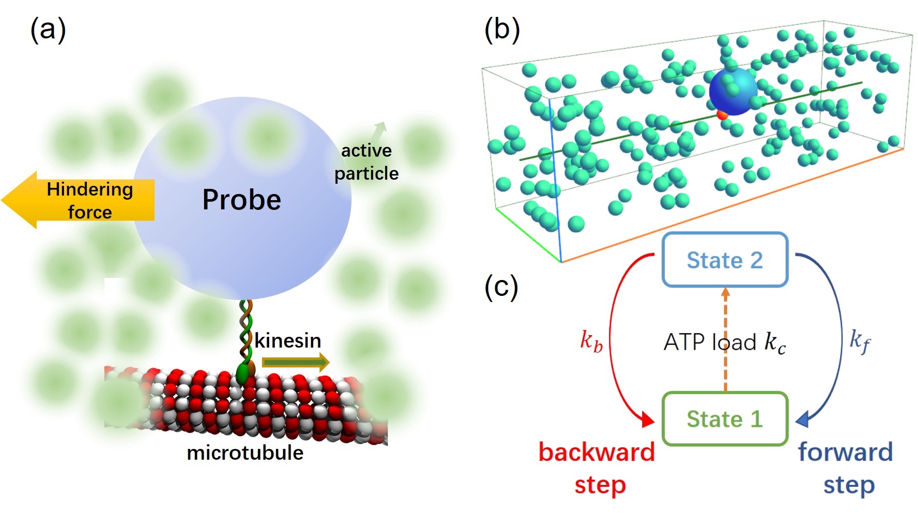
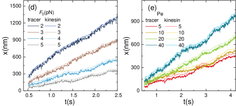
Figure 1: (a)Cartoon for the model system; (b)Schema for actual simulation system: large blue ball stands for the probe, small cyan balls indicate active particles(only a few particles are shown), and red dot indicates the kinesin;(c)Schematic diagram for Markovian model of kinesin movement. Typical trajectories of tracer and kinesin in active bath, (d)for different hindering forces from $-2$ to $-4$ pN with constant activity ${\rm Pe}=40$, (e) for different activity of bath under constant drag force $F_{0}=-4$pN.

II Modeling and Simulations

Let us consider a three-dimensional system shown in Fig.1(a), where a probe (or called tracer elsewhere) attached to a kinesin is suspended in an active bath consisting of $N$ self-propelled particles inside a box of side length $L_{x},L_{y},L_{z}$ with periodic boundaries. These bath particles are propelled by independent OU noises, forced by inter-particle repulsive potentials and background thermal noises. The movement of bath particles is governed by overdamped Langevin equations

$$\dot{{\bf r}}_{i}= -\mu_{b}\nabla_{i}\left[\sum_{j\neq i}V(|{\bf r}_{i}-{\bf r}_{j}|)+U(|{\bf r}_{i}-{\bf x}_{p}|)\right]$$

$$+{\bf f}_{i}+\sqrt{2\mu_{b}k_{B}T}\boldsymbol{\xi}_{i}$$ (1a)

$$\tau_{b}\dot{{\bf f}}_{i}= -{\bf f}_{i}+\sqrt{2D_{b}}\boldsymbol{\zeta}_{i}$$ (1b)

where ${\bf r}_{i}$ is the position for $i$-th bath particle, $\mu_{b}$ is the mobility, ${\bf x}_{p}$ is the position of the probe particle, $V(r)$ and $U(r)$ are interacting potentials between bath-bath particles and bath-probe respectively, ${\bf f}_{i}$ is the propulsion force acting on $i$-bath particle with persistent time $\tau_{b}$ and strength $D_{b}$, $k_{B}$ is Boltzmann constant and $T$ is the background temperature, $\boldsymbol{\xi}_{i}$ and $\boldsymbol{\eta}_{i}$ are independent Gaussian white noise vectors in 3d space, with zero means and delta correlations $\left\langle\boldsymbol{\xi}_{i}(t)\boldsymbol{\xi}_{j}(t^{\prime})\right\rangle=2\delta_{ij}\delta(t-t^{\prime}){\bf I}$ and $\left\langle\boldsymbol{\zeta}_{i}(t)\boldsymbol{\zeta}_{j}(t^{\prime})\right\rangle=2\delta_{ij}\delta(t-t^{\prime}){\bf I}$, where ${\bf I}$ is the unit matrix.

The molecular motor is described by a phenomenological Markov-like kinetic diagram based on experimental observations [19], wherein the complex kinesin walking process is simplified to a two-state Markov transition. In this model, the central ATP hydrolysis and walking process is divided into three transition steps(see Fig.1(c)). The first step is ATP load with constant rate $k_{c}$ and causes a “state transition” (state 1 to state 2). This rate is dependent on the concentration of ATP, and independent of any mechanical issues. The second and third steps are mechanical transitions for forward and backward steps with constant step size $d=8$nm along the microtubule as well as rates $k_{f}$ and $k_{b}$ respectively. Meanwhile the state transition accompanies both steps, from state 2 to state 1. These two rates have both force $F$ dependent as Arrhenius-type

$$k_{\{f,b\}}(F)=k_{\{f,b\}}^{0}\exp\left(\frac{d_{\{f,b\}}F}{k_{B}T}\right)$$ (2)

where $k_{\{f,b\}}^{0}$ is the rate constant without any external force load, $d_{\{f,b\}}$ is the characteristic distant, and all of these parameters are fitted by experimental data. Mathematically, the evolution of the probability of each state ($P_{1}$ and $P_{2}$) obeys a Master equation

$$\frac{{\rm d}}{{\rm d}t}P_{2}=k_{c}P_{1}-(k_{f}+k_{b})P_{2}$$ (3)

This equation establishes the relationship between mean velocity and all fitting parameters for kinesin systems, $\bar{v}=d\frac{(k_{f}-k_{b})k_{c}}{k_{f}+k_{b}+k_{c}}$, which is used to identify fitting parameters mentioned above and can be determined by experiments [17].

One of the most concerned quantities in our model is the position of the probe ${\bf x}_{p}$. The probe is dragged by a constant hindering force ${\bf F}_{0}$ (to mimic optical tweezers in experiments) and pulled by a molecular motor kinesin via a linear spring with stiffness $K$. To illustrate the setup, we draw a cartoon in Fig.1(a), and show the actual simulation system in (b) wherein the kinesin and probe are both constrained to move along $\vec{e}_{x}$ direction. The movement of the probe is also described by an overdamped Langevin equation

$$\dot{x}_{p}=\mu_{p}\left[K(x_{m}-x_{p})+F_{0}+F_{bath}\right]+\sqrt{2\mu_{p}k_{B}T}\xi_{t}$$ (4)

where $x_{p}$ and $x_{m}$ are the position of the probe and the motor along $\vec{e}_{x}$ direction respectively, $\mu_{p}$ is the mobility of the probe, and $F_{bath}=-\frac{\partial}{\partial x_{p}}\sum_{i}U(|{\bf r}_{i}-{\bf x}_{p}|)$ is the interactions between the probe and bath particles.

For easier comparison with the previous experimental results, in simulations we use SI unit and set $k_{B}T=4.115{\rm pN\cdot nm}$ for room temperature. Considering the intracellular environment is dense, and interactions of various components such as proteins and vesicae are soft, we roughly set the active crowder diameter $R_{b}=160$nm and mobility $\mu_{b}=1.0\times 10^{5}{\rm nm/(pN\cdot s)}$, set the bath particle density $\rho=N/(L_{x}L_{y}L_{z})=1.0/R_{b}^{3}$ as a relatively high value, choose harmonic potential as the interactions between particles, $U(r)=\frac{\kappa}{2}(\sigma_{pb}-|r|)^{2}$ for $|r|<\sigma_{pb}$ and $V(r)=\frac{\kappa}{2}(\sigma_{bb}-|r|)^{2}$ for $|r|<\sigma_{bb}$ , where $\sigma_{pb}=(R_{p}+R_{b})/2=340$nm, $\sigma_{bb}=R_{b}=160$nm is the interacting distance of probe-bath particles and bath-bath particles, $\kappa$ is the interaction strength which is set as a constant. Other parameters and simulation details are shown in App.A. In this work, the main control parameters are the activity of active crowder, measured by Péclet number, which is dimensionless and defined as ${\rm Pe}=\frac{\sqrt{D_{b}/\tau_{b}}R_{b}}{\mu_{b}k_{B}T}$, where $\sqrt{D_{b}/\tau_{b}}$ is standard deviation of ${\bf f}_{i}$, as well as the persistent time of active crowder $\tau_{b}$.

Figure1(d,e) shows several typical simulation trajectories of the kinesin and the probe attached to it. Due to the kinesin walking process, all kinesin/probe moves toward positive $x$ direction. With the constant bath activity and kinetics parameters of kinesin, the influence of hindering load force on kinesin/probe movement is shown in Fig.1(d). As a matter of course, larger load force leads to slower movement, as well as larger distance between kinesin and probe. Besides, the active fluctuations on probe contribute significant promotion effect. As shown in Fig.1(e), with the constant hindering force, larger bath activity induces faster kinesin/probe movement.

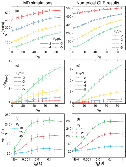
Figure 2: (a)Simulation results, average velocity of the probe in the active bath of activity. Each marker indicates various average loads from $-2$ to $-5$pN; (b)Numerical solution of GLE with the same conditions and parameters as (a); (c,d)Relative velocity of the probe under the same parameters with (a,b) respectively; (e,f)Probe velocity for various activity Pe, figures are the plots of $v$ as the function of persistent time $\tau_{b}$. Other parameters herein: for (a)-(d), we use $\tau_{b}=0.01{\rm s}\approx\frac{R_{b}^{2}}{6\mu_{b}k_{B}T}$, which is the characteristic rotational time of a Brownian particle with diameter $R_{b}$. All figures use $\kappa=0.003{\rm pN/nm}$ that indicates a weak interaction, we also test other values of $\kappa$, qualitatively results are not affected by this parameter.

Average velocities of probe $v$ for variant bath activities are shown in Fig.2(a) and (c) for a normalized version, and each marker indicates the hindering force $F_{0}$ from $-2$ to $-5$pN. Results show that probe velocity $v$ increases with bath activity Pe monotonically in all cases. Especially, normalized velocity $v/v_{{\rm Pe=0}}$ shows a stronger enhancement under high hindrance loads. This result is very similar to a most recent in vitro experiment [17], wherein the researchers have used optical tweezers to apply a “semitruncated Lévy noise” and an additional constant load force on the probe. They found that motor/probe velocity increases with the magnitude of the noise, and that such increases are larger for the stronger load forces. We also investigate the kinesin velocity dependence on persistent time of active bath particles with fixed activity Pe, shown in Fig.2(e). Simulations show that the probe velocity increases with persistent time $\tau_{b}$ at first and next reaches a platform. Then, probe velocity weakly decreases at large $\tau_{b}$ region.

III Theory of Active Bath

To understand our simulation results, we develop a mean-field theory method to investigate the system theoretically. The starting point of the theory is the overdamped Langevin equations (1), and the objective of the theory is to obtain an effective movement equation that only contains probe and kinesin variables. To eliminate numerous degrees of freedom of bath particles, we describe the model system at a coarse-grained level, employing an evolution equation for bath particles’ density profile $\rho({\bf r},t)$

$$\frac{\partial\rho({\bf r},t)}{\partial t}= \mu_{b}\nabla_{{\bf r}}\cdot\rho({\bf r},t)\nabla_{{\bf r}}\Big{[}\int\rho({\bf r}^{\prime},t)V(|{\bf r}-{\bf r}^{\prime}|){\rm d}{\bf r}^{\prime}$$

$$+U(|{\bf r}-{\bf x_{p}}|)\Big{]}+\nabla\cdot\left[\sqrt{\rho({\bf r},t)}\boldsymbol{\xi}^{A}({\bf r},t)\right]$$ (5)

$$+\nabla\cdot\left[\sqrt{\rho({\bf r},t)}\boldsymbol{\xi}^{T}({\bf r},t)\right]+\mu_{b}k_{B}T\nabla^{2}\rho({\bf r},t)$$

which is a Dean-like equation for active particle system, wherein $\boldsymbol{\xi}^{A,T}\left({\bf r},t\right)$ are noise filed functions. To embody the effect of such density profile on probe movement, we firstly solve this equation in Fourier space formally,

$$\frac{\partial\rho_{k}(t)}{\partial t} \approx-\mu_{b}k^{2}\left[(k_{B}T+\rho V_{k})\rho_{k}(t)+\rho U_{k}e^{i{\bf k}\cdot{\bf x}_{p}}\right]$$

$$+i\sqrt{\rho}{\bf k}\cdot\left[\tilde{\boldsymbol{\xi}}^{T}({\bf k},t)+\tilde{\boldsymbol{\xi}}^{A}({\bf k},t)\right]$$ (6)

where $\rho$ is the number density of bath particle, $\tilde{\boldsymbol{\xi}}^{A,T}({\bf k},t)$, $U_{k},V_{k}$ are Fourier transform of noises $\boldsymbol{\xi}^{A,T}({\bf r},t)$ and potentials $U(r),V(r)$ respectively, with time correlations $\left\langle\tilde{\xi}_{\alpha}^{A*}({\bf k},t)\tilde{\xi}_{\beta}^{A}({\bf k}^{\prime},t^{\prime})\right\rangle=\frac{D_{b}}{\tau_{b}}\delta_{\alpha\beta}(2\pi)^{3}\delta({\bf k}-{\bf k}^{\prime})e^{-|t-t^{\prime}|/\tau_{b}}$ and $\left\langle\tilde{\xi}_{\alpha}^{T*}({\bf k},t)\tilde{\xi}_{\beta}^{T}({\bf k}^{\prime},t^{\prime})\right\rangle=2\mu_{b}k_{B}T\delta_{\alpha\beta}(2\pi)^{3}\delta({\bf k}-{\bf k}^{\prime})\delta(t-t^{\prime})$. Then insert this formal solution into Eq.(4) by utilizing an identity $-\nabla_{{\bf x}_{p}}\sum_{i}U(|{\bf r}_{i}-{\bf x}_{p}|)\equiv\frac{1}{(2\pi)^{3}}\int i{\bf k}e^{-i{\bf k}\cdot{\bf x}_{p}}\rho_{k}(t)U_{k}{\rm d}^{3}{\bf k}$. After some appropriate approximations, we obtain a generalized Langevin equation for the probe

$$\dot{x}_{p}(t)= -\mu_{p}\int_{-\infty}^{t}\zeta(t-s)\dot{x}_{p}(s){\rm d}s+\eta_{A}(t)+\eta_{T}(t)$$

$$+\mu_{p}[K(x_{m}-x_{p})+F_{0}]+\sqrt{2\mu_{p}k_{B}T}\xi_{t}$$ (7)

with memory kernel

$$\zeta(t)=\frac{\mu_{p}\mu_{b}\rho}{3(2\pi)^{3}}\int k^{4}U_{k}^{2}a_{k}e^{-t/a_{k}}{\rm d}^{3}{\bf k}$$ (8)

where $a_{k}=\left[\mu_{b}k^{2}(k_{B}T+\rho V_{k})\right]^{-1}$ is a characteristic time scale, and $\eta_{A,T}$ are complicated colored noise

$$\eta_{A,T}(t)= \frac{\mu_{p}\sqrt{\rho}}{(2\pi)^{3}}\int ik_{x}U_{k}$$

$$\times\int_{-\infty}^{t}e^{-(t-s)/a_{k}}{\bf k}\cdot\tilde{\boldsymbol{\xi}}^{A,T}({\bf k},s){\rm d}s{\rm d}^{3}{\bf k}$$ (9)

with time correlation functions

$$\left\langle\eta_{T}(t)\eta_{T}(t^{\prime})\right\rangle =\frac{\mu_{t}^{2}\rho\mu_{b}k_{B}T}{3(2\pi)^{3}}\int U_{k}^{2}k^{4}a_{k}e^{-|t-t^{\prime}|/a_{k}}{\rm d}^{3}{\bf k}$$ (10a)

$$\left\langle\eta_{A}(t)\eta_{A}(t^{\prime})\right\rangle =\frac{\mu_{t}^{2}\rho D_{b}}{3(2\pi)^{3}}\int U_{k}^{2}k^{4}\frac{1}{(\tau_{b}/a_{k})^{2}-1}$$

$$\times\left[\tau_{b}e^{-|t-t^{\prime}|/\tau_{b}}-a_{k}e^{-|t-t^{\prime}|/a_{k}}\right]{\rm d}^{3}{\bf k}$$ (10b)

Herein, a generalized fluctuation-dissipation relationship (FDR) is reveal between memory kernel $\zeta(t)$ and noise $\eta_{T}$, and the OU noise of the bath particle brings an explicitly violation of the FDR. When the activity of the bath is absent, Eq.(7) reduces to a GLE in equilibrium and the FDR holds naturally.

Equations (7)-(9) are main theoretical results of the present work. They unravel the properties of noise generated by active environment, and allow us to directly calculate the probe movement and average velocity. Numerical solutions of Eq.(7) are shown in Fig.2(b), (d) and (f), wherein the parameters are chosen same as (a),(c) and (e) respectively. Compared with simulation results, the GLE reproduces the acceleration effect of active crowders (a)-(d), quantitatively in most cases. Surprisingly, GLE solutions also show very similar behavior of relationship between probe velocity and persistent time $\tau_{b}$, which further confirms the non-trivial phenomenon.

Theoretical explanations about the mechanism of kinesin acceleration are still in development. In Ref.[17], the authors pointed out that the amplitude of noise is a major factor. Yet in a ratchet potential model [20], not only the noise strength significantly influence the probe dynamics, but also non-Gaussian property and time correlation behavior of the noise. Herein, with the help of the GLE, it is feasible to investigate which property of the noise dominates kinesin acceleration.

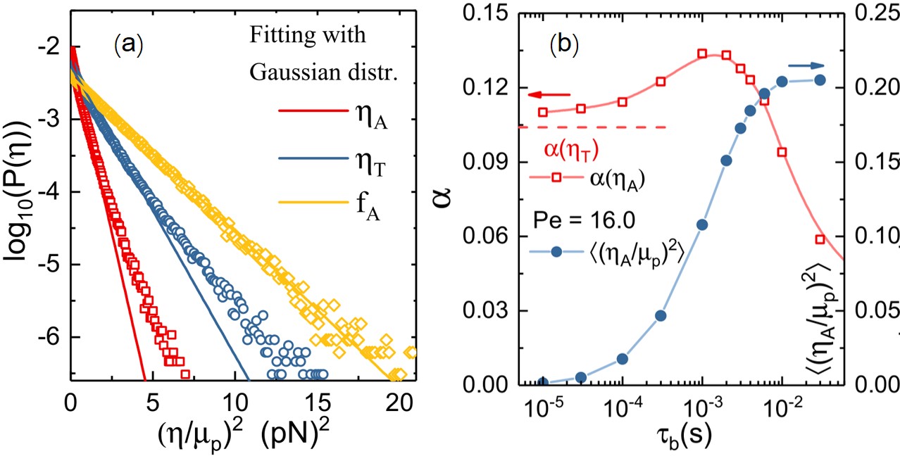
Figure 3: (a) Distributions for noise $\boldsymbol{\eta}_{A}$ (red squares) and $\boldsymbol{\eta}_{T}$ (blue round dots), solid lines are fitting lines with hypothetical Gaussian distributions. ${\rm f}_{A}$ is an OU process as a reference(yellow diamonds and line), which satisfies an exact Gaussian distribution. Herein, we set $\tau_{b}=0.01{\rm s}$. (b) Non-Gaussian parameters $\alpha$ for $\boldsymbol{\eta}_{A}$ and $\boldsymbol{\eta}_{T}$ (red squares and left vertical axis), the formal one depends on persistent $\tau_{b}$ which is drawn here as horizontal axis. Also, we plot the variance of noise $\boldsymbol{\eta}_{A}/\mu_{p}$ (blue points and right vertical axis). Other parameters for all subplots: $\kappa=0.01{\rm pN/nm}$, ${\rm Pe}=16.0$.

Firstly, we focus on the strength (or amplitude) of the colored noise $\eta_{A,T}(t)$. According to Eq.(9), or more straightforwardly, the time correlation function of $\eta_{A,T}(t)$, the explicit expression for variance

$$\left\langle\eta_{T}^{2}\right\rangle= \frac{\mu_{t}^{2}\rho\mu_{b}k_{B}T}{3(2\pi)^{3}}\int U_{k}^{2}k^{4}a_{k}{\rm d}^{3}{\bf k},$$ (11a)

$$\left\langle\eta_{A}^{2}\right\rangle= \frac{\mu_{t}^{2}\rho D_{b}}{3(2\pi)^{3}}\int\frac{U_{k}^{2}k^{4}a_{k}^{2}}{\tau_{b}+a_{k}}{\rm d}^{3}{\bf k},$$ (11b)

can be obtained, therefore $\left\langle\eta_{A}^{2}\right\rangle\propto{\rm Pe}^{2}\tau_{b}\int\frac{k^{4}U_{k}^{2}a_{k}^{2}}{\tau_{b}+a_{k}}{\rm d}^{3}{\bf k}$. As shown in Fig.2(b) and (d), probe velocity $v$ increases with Pe monotonically when $\tau_{b}$ is constant. Although the analytical relation between $v$ and Pe is not given due to the complexity of memory kernel and colored noise, qualitatively variance of noise $\eta_{A}$ definitely makes a positive contribution to kinesin acceleration.

Another quantity we concerned is the non-Gaussian property of these two colored noises. To intuitively show the distributions of such noises, we plot the probability distribution function $P(\eta)$ in Fig.3(a). Red square and blue round hollow dots represent $\eta_{A}$ and $\eta_{T}$ respectively, and solid curves are their Gaussian fitting. Interestingly, both $\eta_{T}$ and $\eta_{A}$ show heavy tail distributions and clearly deviate from Gaussian distributions. As a contrast, the distribution function of OU noise ${\rm f}_{A}$ is also plotted with yellow diamond dots, which perfectly satisfies Gaussian distribution. Noticing that Lévy noise also have such heavy tail distribution[17], as well as the ECP noise[20], they all have non-trivial acceleration effect on kinesin. To quantitatively investigate this property, we then calculate the non-Gaussian parameter $\alpha(\eta)=\frac{\left\langle\eta^{4}\right\rangle}{3\left\langle\eta^{2}\right\rangle^{2}}-1$ of $\eta_{A,T}(t)$. These quantities are not functions of temperature $T$ nor activity Pe, therefore the contribution of non-Gaussian property cannot be seen in Fig.2(a)-(d). Yet $\alpha(\eta_{A})$ is a function of $\tau_{b}$, and both simulation and GLE solution show the same dependency relationship of kinesin velocity on $\tau_{b}$. Hence we plot non-Gaussian parameter $\alpha$ (red squares, left axis) and corresponding noise variance (blue dots, right axis) as functions of persistent time $\tau_{b}$ in Fig.3(b). When $\tau_{p}\rightarrow 0$, $\eta_{A}$ reduces to the noise $\eta_{T}$ (under an effective temperature $T_{{\rm eff}}=D_{b}/(\mu_{b}k_{B})$), and its non-Gaussian parameter is shown as a red horizontal dash line in Fig.3(b). As $\tau_{b}$ increases, $\left\langle\eta_{A}^{2}\right\rangle$ monotonically increases and then reaches to a plateau, which is very similar to the velocity increase with $\tau_{b}$ at short and mediate region. As shown in Fig.2(e,f), when $\tau_{b}$ is large enough, the kinesin velocity slightly decreases with $\tau_{b}$. This weak decrease behavior has not be seen in the noise variance. On the contrary, a strongly non-monotonic dependence of $\alpha(\eta_{A})$ on $\tau_{b}$ is observed. The non-Gaussian parameter $\alpha(\eta_{A})$ rapidly decreases with $\tau_{b}$ when it is large. This phenomenon is very likely to lead to the weak decrease of the kinesin velocity. In general, variance indeed make the major contribution to the kinesin acceleration, while non-Gaussian property also makes a minor yet positive contribution to it.

IV Conclusion

In summary, we build a bottom-up model consisting of a Markovian kinesin model and an active particle bath to investigate the acceleration behavior of kinesin and probe attached to it in complex intracellular environment. Simulations show kinesin velocity increases with bath activity monotonically, especially for larger load situations where more significant acceleration effect is observed. We also establish a coarse-grained theoretical framework to describe the active bath and obtain a generalized Langevin equation for probe movement. The effects of active bath on the probe are simplified into a memory kernel and two effective noises. Numerical calculations of the GLE show very good agreement with simulation data. Furthermore, the introduction of the theory allows us to study the noise property conveniently and to investigate which one of them is the essential to kinesin acceleration. Comparing simulations and numerical solutions for GLE, we find out that the variance of noise plays a major role in kinesin acceleration, while non-Gaussian property brings positive yet minor contributions.

Our model and theory bring a novel, quantifiable research approach to active fluctuations in living cells, which bridges between phenomenological description of kinesin movement and underlying principles of statistical physics. For further study, with more information input such as accurate interacting parameters, we believe our model could give more accurate results, and deeper understanding on the noise property. In addition, the theory of active bath is independent of the kinesin model, which also serves as a new way to investigate active environment. The generality of which could lead to numerous other applications in other probe-bath interacting systems.

V Acknowledgement

This work is supported by MOST(2018YFA0208702) and NSFC (32090044, 21833007).

 

Appendix A Numerical Simulations

Numerical simulations are run in a three-dimensional box $(L_{x},L_{y},L_{z})=(40\sigma,10\sigma,10\sigma)$ with periodic boundary, where $\sigma=160$nm as the unit of length. In the present coarse-grained model, both the kinesin and the probe’s movements are constrained on a fixed line $(y,z)=(L_{y}/2,L_{z}/2)$. The volume repulsive interactions are only considered between bath-bath particles and bath-probe, meaning that the kinesin’s volume repulsive interaction is not considered. The diameter of bath particle and the probe are set as $R_{b}=\sigma,R_{p}=3.25\sigma$, so that inter-particle distance $\sigma_{pb}=2.125\sigma$. The temperature is set as the room temperature, therefore $k_{B}T=4.115{\rm pN\cdot nm}$, which is used as the unit of the energy. The mobility of bath particle is $\mu_{b}=1.0\times 10^{5}{\rm nm/(pN\times s)}$, which can be used to label the unit of time $\tau_{u}=\sigma^{2}/(\mu_{b}k_{B}T)=6.22\times 10^{-2}{\rm s}$. We set the probe diameter $R_{p}=520$nm and mobility $\mu_{p}=0.308\times 10^{5}{\rm nm/(pN\cdot s)}$.

In simulations, we use the time step $\delta t=5.0\times 10^{-6}{\rm s}$ (to keep $k_{c,b,f}\delta t\ll 1$, $\delta_{t}\ll\tau_{b}$ and $\delta t\ll\tau_{u}$). For each time interval, both the Markovian dynamics for kinesin and the Langevin dynamics for probe and bath particles are performed. For each simulation, the system is allowed to reach a steady state over $10^{6}\delta t$, and then the kinesin/probe’s displacements and velocities are averaged over following $10^{7}\delta t$ time interval. The variance of the velocity is calculated by at least 20 times simulations with the exact same parameters and different random number seeds. We find that more average counts did not have a significant effect on the reduction of the variance.

For the numerical calculation of the GLE, the time step is also set as $\delta t=5.0\times 10^{-6}{\rm s}$. The generation of the complex color noises is shown in App.C. Velocities and their variances are calculated by over $10^{7}$ time steps and 50 trajectories.

The Markov transition migrates from Ref.[17], and parameters in Eqs.2 and 3 also come from this reference: $k_{f}^{0}=1002{\rm s^{-1}}$, $k_{b}^{0}=27.9{\rm s^{-1}}$, $k_{c}=102{\rm s^{-1}}$, $d_{f}=3.61{\rm nm}$, $d_{b}=1.14{\rm nm}$.

Appendix B Dean’s equation for active bath and effective generalized Langevin equation for probe

This section gives the derivation details of Eq.(4) in main text. The starting point is the Langevin equation for bath particles

$$\dot{{\bf r}}_{i}= -\mu_{b}\nabla_{i}\left[\sum_{j\neq i}V(|{\bf r}_{i}-{\bf r}_{j}|)+U(|{\bf r}_{i}-{\bf x}_{p}|)\right]+{\bf f}_{i}+\sqrt{2\mu_{b}k_{B}T}\boldsymbol{\xi}_{i}$$ (12a)

$$\tau_{b}\dot{{\bf f}}_{i}= -{\bf f}_{i}+\sqrt{2D_{b}}\boldsymbol{\eta}_{i}$$ (12b)

Introducing the single particle density $\rho_{i}({\bf r},t)=\delta({\bf r}-{\bf r}_{i}(t))$ and the collective one $\rho({\bf r},t)=\sum_{i=1}^{N}\rho_{i}({\bf r},t)$, for an arbitrary function of bath particle coordinate $g({\bf r}_{i})$ with natural boundary condition, according to the Itō calculus, one has

$$\frac{{\rm d}g({\bf r}_{i})}{{\rm d}t}= \left\{-\mu_{b}\nabla_{i}\left[\sum_{j\neq i}V(|{\bf r}_{i}-{\bf r}_{j}|)+U(|{\bf r}_{i}-{\bf x_{p}}|)\right]+{\bf f}_{i}+\sqrt{2\mu_{b}k_{B}T}\boldsymbol{\xi}_{i}\right\}\cdot\nabla_{i}g({\bf r}_{i})$$

$$+\mu_{b}k_{B}T\nabla_{i}^{2}g({\bf r}_{i})$$

$$= \int\rho_{i}({\bf r},t)\Bigg{\{}\left(-\mu_{b}\nabla_{{\bf r}}\left[\sum_{j\neq i}V(|{\bf r}-{\bf r}_{j}|)+U(|{\bf r}-{\bf x_{p}}|)\right]+{\bf f}_{i}+\sqrt{2\mu_{b}k_{B}T}\boldsymbol{\xi}_{i}\right)\cdot\nabla_{{\bf r}}g({\bf r})$$

$$+\mu_{b}k_{B}T\nabla_{{\bf r}}^{2}g({\bf r})\Bigg{\}}{\rm d}{\bf r}$$

$$= \int\rho_{i}({\bf r},t)\Bigg{\{}\left[-\mu_{b}\nabla_{{\bf r}}\left[\int\rho({\bf r}^{\prime},t)V(|{\bf r}-{\bf r}^{\prime}|){\rm d}{\bf r}^{\prime}+U(|{\bf r}-{\bf x_{p}}|)\right]+{\bf f}_{i}+\sqrt{2\mu_{b}k_{B}T}\boldsymbol{\xi}_{i}\right]\cdot\nabla_{{\bf r}}g({\bf r})$$

$$+\mu_{b}k_{B}T\nabla_{{\bf r}}^{2}g({\bf r})\Bigg{\}}{\rm d}{\bf r}$$

$$= \int g({\bf r})\Bigg{\{}\nabla_{{\bf r}}\cdot\left[\mu_{b}\nabla_{{\bf r}}\left[\int\rho({\bf r}^{\prime},t)V(|{\bf r}-{\bf r}^{\prime}|){\rm d}{\bf r}^{\prime}+U(|{\bf r}-{\bf x_{p}}|)\right]-{\bf f}_{i}-\sqrt{2\mu_{b}k_{B}T}\boldsymbol{\xi}_{i}\right]\rho_{i}({\bf r},t)$$

$$+\mu_{b}k_{B}T\nabla_{{\bf r}}^{2}\rho_{i}({\bf r},t)\Bigg{\}}$$ (13)

In the third step it seems there is an extra term $V(0)$, but it vanishes due to $\nabla_{{\bf r}}$ operator, and the last step used part integral. On the other hand, with the identity $\frac{{\rm d}}{{\rm d}t}g({\bf r}_{i})=\frac{{\rm d}}{{\rm d}t}\int\rho_{i}({\bf r},t)g({\bf r}){\rm d}{\bf r}=\int\frac{\partial\rho_{i}({\bf r},t)}{\partial t}g({\bf r}){\rm d}{\bf r}$, and considering the arbitrariness of function $g({\bf r})$, immediately

$$\frac{\partial\rho_{i}({\bf r},t)}{\partial t}= \nabla_{{\bf r}}\cdot\rho_{i}({\bf r},t)\left[\mu_{b}\nabla_{{\bf r}}\left[\int\rho({\bf r}^{\prime},t)V(|{\bf r}-{\bf r}^{\prime}|){\rm d}{\bf r}^{\prime}+U(|{\bf r}-{\bf x_{p}}|)\right]-{\bf f}_{i}-\sqrt{2\mu_{b}k_{B}T}\boldsymbol{\xi}_{i}\right]$$

$$+\mu_{b}k_{B}T\nabla_{{\bf r}}^{2}\rho_{i}({\bf r},t)$$ (14)

then the collective density function

$$\frac{\partial\rho({\bf r},t)}{\partial t}= \mu_{b}\nabla\cdot\left[\rho({\bf r},t)\nabla\left(\int\rho({\bf r}^{\prime},t)V(|{\bf r}-{\bf r}^{\prime}|)+U(|{\bf r}-{\bf x}_{p}|)\right)\right]$$

$$+\sum_{i}\left[-\nabla\cdot({\bf f}_{i}\rho_{i})-\sqrt{2\mu_{b}k_{B}T}\nabla\cdot(\rho_{i}\boldsymbol{\xi}_{i})\right]+\mu_{b}k_{B}T\nabla^{2}\rho({\bf r},t)$$ (15)

This equation is not self-consistent yet, since ${\bf f}_{i}\rho_{i}$ and $\rho_{i}\boldsymbol{\xi}_{i}$ terms still exist. To fix this, following Dean’s method [49], we introduce two noise fields $\chi_{1,2}({\bf r},t)$ as functions of $\rho({\bf r},t)$ to replace $\chi_{1}^{\prime}({\bf r},t)=-\sum_{i}\nabla\cdot({\bf f}_{i}\rho_{i})$ and $\chi_{2}^{\prime}({\bf r},t)=-\sqrt{2\mu_{b}k_{B}T}\sum_{i}\nabla\cdot(\rho_{i}\boldsymbol{\xi}_{i})$. Considering

$$\left\langle\chi_{1}^{\prime}({\bf r},t)\chi_{1}^{\prime}({\bf r}^{\prime},t^{\prime})\right\rangle= \frac{D_{b}}{\tau_{b}}e^{-|t-t^{\prime}|/\tau_{b}}\sum_{i}\nabla\cdot\nabla^{\prime}\left[\rho_{i}({\bf r},t)\rho_{i}({\bf r}^{\prime},t^{\prime})\right]$$

$$= \frac{D_{b}}{\tau_{b}}e^{-|t-t^{\prime}|/\tau_{b}}\nabla\cdot\nabla^{\prime}\left[\rho({\bf r},t)\delta({\bf r}-{\bf r}^{\prime})\right],$$ (16a)

$$\left\langle\chi_{2}^{\prime}({\bf r},t)\chi_{2}^{\prime}({\bf r}^{\prime},t^{\prime})\right\rangle= 2\mu_{b}k_{B}T\delta(t-t^{\prime})\sum_{i}\nabla\cdot\nabla^{\prime}\left[\rho_{i}({\bf r},t)\rho_{i}({\bf r}^{\prime},t^{\prime})\right]$$

$$= 2\mu_{b}k_{B}T\delta(t-t^{\prime})\nabla\cdot\nabla^{\prime}\left[\rho({\bf r},t)\delta({\bf r}-{\bf r}^{\prime})\right],$$ (16b)

we construct noise field $\chi_{1}({\bf r},t)=\nabla\cdot\left[\sqrt{\rho({\bf r},t)}\boldsymbol{\xi}^{A}({\bf r},t)\right]$ and $\chi_{2}({\bf r},t)=\nabla\cdot\left[\sqrt{\rho({\bf r},t)}\boldsymbol{\xi}^{T}({\bf r},t)\right]$ to keep the correlations of $\chi_{1}$ and $\chi_{1}^{\prime}$, $\chi_{2}$ and $\chi_{2}^{\prime}$ equal, where $\boldsymbol{\xi}^{A,T}({\bf r},t)$ are also noise field with correlation $\left\langle\boldsymbol{\xi}^{A}({\bf r},t)\boldsymbol{\xi}^{A}({\bf r}^{\prime},t^{\prime})\right\rangle=\frac{D_{b}}{\tau}e^{-|t-t^{\prime}|/\tau_{b}}\delta({\bf r}-{\bf r}^{\prime}){\bf I}$ and $\left\langle\boldsymbol{\xi}^{T}({\bf r},t)\boldsymbol{\xi}^{T}({\bf r}^{\prime},t^{\prime})\right\rangle=2\mu_{b}k_{B}T\delta(-|t-t^{\prime}|)\delta({\bf r}-{\bf r}^{\prime}){\bf I}$ respectively. Now we achieve a self-consistent equation for the evolution of $\rho({\bf r},t)$

$$\frac{\partial\rho({\bf r},t)}{\partial t}= \mu_{b}\nabla_{{\bf r}}\cdot\rho({\bf r},t)\nabla_{{\bf r}}\left[\int\rho({\bf r}^{\prime},t)V(|{\bf r}-{\bf r}^{\prime}|){\rm d}{\bf r}^{\prime}+U(|{\bf r}-{\bf x_{p}}|)\right]$$

$$+\mu_{b}k_{B}T\nabla^{2}\rho({\bf r},t)+\nabla\cdot\left[\sqrt{\rho({\bf r},t)}\boldsymbol{\xi}^{A}({\bf r},t)\right]+\nabla\cdot\left[\sqrt{\rho({\bf r},t)}\boldsymbol{\xi}^{T}({\bf r},t)\right]$$ (17)

This equation is one of the central results in this section, also known as Dean’s equation.

To eliminate variables of bath particle positions, we use a mean-field theory to describe the active bath. Using Eq.17 and assuming the environment is isotropic, homogeneous and no special structures(suitable for weak interaction and dense situations), the evolution equation for bath density can be simplified as

$$\frac{\partial\rho_{k}(t)}{\partial t}\approx-\mu_{b}k^{2}\left[(k_{B}T+\rho V_{k})\rho_{k}(t)+\rho U_{k}e^{i{\bf k}\cdot{\bf x}_{p}}\right]+i\sqrt{\rho}{\bf k}\cdot\left[\tilde{\boldsymbol{\xi}}^{T}({\bf k},t)+\tilde{\boldsymbol{\xi}}^{A}({\bf k},t)\right]$$ (18)

in Fourier space, where $\rho_{k}(t)$, $U_{k}$, $V_{k}$, $\tilde{\boldsymbol{\xi}}^{A}({\bf k},t)$ and $\tilde{\boldsymbol{\xi}}^{T}({\bf k},t)$ are Fourier transforms of $\rho({\bf r},t)$, $U(r),V(r),\boldsymbol{\xi}^{A}({\bf r},t)$ and $\boldsymbol{\xi}^{T}({\bf r},t)$ respectively. This equation has a formal solution

$$\rho_{k}(t)=\int_{-\infty}^{t}e^{-(t-s)/a_{k}}\left[-\mu_{b}k_{B}Tk^{2}\rho U_{k}e^{i{\bf k}\cdot{\bf x}_{p}}+i\sqrt{\rho}{\bf k}\cdot(\tilde{\boldsymbol{\xi}}^{A}({\bf k},s)+\tilde{\boldsymbol{\xi}}^{T}({\bf k},s))\right]{\rm d}s$$ (19)

where $a_{k}=\left[\mu_{b}k^{2}(k_{B}T+\rho V_{k})\right]^{-1}$. Using the identity (performing Fourier transition and its inverse transform on the l.h.s.)

$$-\nabla_{{\bf x}_{p}}\sum_{i}U(|{\bf r}_{i}-{\bf x}_{p}|)\equiv\frac{1}{(2\pi)^{3}}\int i{\bf k}e^{-i{\bf k}\cdot{\bf x}_{p}}\rho_{k}(t)U_{k}{\rm d}^{3}{\bf k},$$ (20)

and inserting the formal solution (19) into the Langevin equation for probe Eq.(1) in main text, we get a generalized Langevin equation for probe movement along $\vec{e}_{x}$-direction.

$$\dot{x}_{p}=\mu_{p}\int_{-\infty}^{t}\tilde{F}(t-s){\rm d}s+\mu_{p}[K(x_{m}-x_{p})+F_{0}]+\eta_{A}(x_{p}(t),t)+\eta_{T}(x_{p}(t),t)+\sqrt{2\mu_{p}k_{B}T}\xi_{t}$$ (21)

where $\tilde{F}(t)=-\frac{\mu_{b}\rho}{(2\pi)^{3}}\int ik_{x}k^{2}U_{k}^{2}e^{-ik_{x}[x_{p}(t)-x_{p}(s)]}e^{-(t-s)/a_{k}}$ is a complex memory kernel, and

$$\eta_{A,T}(x_{p}(t),t)=\frac{\mu_{p}\sqrt{\rho}}{(2\pi)^{3}}\int ik_{x}U_{k}e^{-ik_{x}x_{p}(t)}\int_{-\infty}^{t}e^{-(t-s)/a_{k}}{\bf k}\cdot\tilde{\boldsymbol{\xi}}^{A,T}({\bf k},s){\rm d}s{\rm d}^{3}{\bf k}$$ (22)

is the colored noise term induced by bath. This memory kernel is far complex to use, yet to the linear order, the memory kernel can be simplified to the form $\mu_{p}\int_{-\infty}^{t}\tilde{F}(t-s){\rm d}s\approx-\int_{-\infty}^{t}\zeta(t-s)\dot{x}_{p}(s){\rm d}s$, where

$$\zeta(t)=\frac{\mu_{p}\mu_{b}\rho}{3(2\pi)^{3}}\int k^{4}U_{k}^{2}a_{k}e^{-t/a_{k}}{\rm d}^{3}{\bf k}$$ (23)

which is much easier to employ. As for the noise $\eta_{A,T}(x_{p}(t),t)$, considering the time scale of probe movement is much slower than bath particles, we use the adiabatic approximation so that the noises can be simplified into

$$\eta_{A,T}(t)=\frac{\mu_{p}\sqrt{\rho}}{(2\pi)^{3}}\int ik_{x}U_{k}\int_{-\infty}^{t}e^{-(t-s)/a_{k}}{\bf k}\cdot\tilde{\boldsymbol{\xi}}^{A,T}({\bf k},s){\rm d}s{\rm d}^{3}{\bf k}$$ (24)

with time correlations

$$\left\langle\eta_{T}(t)\eta_{T}(t^{\prime})\right\rangle =\frac{2\mu_{t}^{2}\rho\mu_{b}k_{B}T}{(2\pi)^{3}}\int k_{x}^{2}U_{k}^{2}k^{2}\frac{a_{k}}{2}e^{-|t-t^{\prime}|/a_{k}}{\rm d}^{3}{\bf k}$$ (25a)

$$\left\langle\eta_{A}(t)\eta_{A}(t^{\prime})\right\rangle =\frac{\mu_{t}^{2}\rho D_{b}}{(2\pi)^{3}}\int k_{x}^{2}U_{k}^{2}k^{2}\frac{1}{(\tau_{b}/a_{k})^{2}-1}\left[\tau_{b}e^{-|t-t^{\prime}|/\tau_{b}}-a_{k}e^{-|t-t^{\prime}|/a_{k}}\right]{\rm d}^{3}{\bf k}$$ (25b)

Appendix C Generation of Complex Colored Noise

According to Eq.(24), and using Greek alphabet to express vector component, $\boldsymbol{\eta}_{A,T}$ in $\alpha$ component is

$$\eta_{A,T}^{\alpha}(t)=\frac{\mu_{t}\sqrt{\rho}}{(2\pi)^{3}}\int{\rm d}^{3}{\bf k}k^{\alpha}e^{-i{\bf k}\cdot{\bf x}_{p}(t)}U_{k}\int_{-\infty}^{t}e^{-(t-s)/a_{k}}[\sum_{\beta}k^{\beta}\tilde{\xi}^{A,T}_{\beta}({\bf k},s)]{\rm d}s$$ (26)

Since $\tilde{\xi}_{\beta}^{A,T}({\bf k},t)=\int{\xi}^{A,T}_{\beta}({\bf r},t)e^{i{\bf k}\cdot{\bf r}}{\rm d}^{3}{\bf r}$, as well as the correlations shown in Sec.B, one has

$$\left\langle\tilde{\xi}^{A*}_{\alpha}({\bf k},t)\tilde{\xi}^{A}_{\beta}({\bf k}^{\prime},t^{\prime})\right\rangle =\frac{D_{b}}{\tau_{b}}\delta_{\alpha\beta}(2\pi)^{3}\delta({\bf k}-{\bf k}^{\prime})e^{-|t-t^{\prime}|/\tau_{b}}$$ (27a)

$$\left\langle\tilde{\xi}^{T*}_{\alpha}({\bf k},t)\tilde{\xi}^{T}_{\beta}({\bf k}^{\prime},t^{\prime})\right\rangle =2\mu_{b}k_{B}T\delta_{\alpha\beta}(2\pi)^{3}\delta({\bf k}-{\bf k}^{\prime})\delta(t-t^{\prime})$$ (27b)

Therefore random variables $\tilde{\xi}^{A,T}_{\alpha}({\bf k},t)$ can be devided into two independent stochastic processes in time and $k$ space,

$$\tilde{\xi}^{A}_{\alpha}({\bf k},t){\rm d}t{\rm d}^{3}{\bf k} =\sqrt{\frac{D_{b}}{\tau_{b}}}(2\pi)^{3/2}f_{\alpha}(t){\rm d}t{\rm d}^{3}W_{{\bf k}}$$ (28a)

$$\tilde{\xi}^{T}_{\alpha}({\bf k},t){\rm d}t{\rm d}^{3}{\bf k} =\sqrt{2\mu_{b}k_{B}T}(2\pi)^{3/2}{\rm d}W_{t}{\rm d}^{3}W_{{\bf k}}$$ (28b)

where $W_{t}$ and $W_{{\bf k}}$ are independent Wiener processes, $f_{\alpha}(t)$ is an dimensionless OU process with $\tau_{b}\dot{f}_{\alpha}(t)=-f_{\alpha}(t)+\sqrt{2\tau_{b}}\xi_{t}$ ($\xi_{t}$ stands for standard white noise), formal solution $f_{\alpha}(t)=\sqrt{\frac{2}{\tau_{b}}}\int_{-\infty}^{t}e^{-(t-s)/\tau_{b}}\xi_{s}{\rm d}s$ and time correlation $\left\langle f_{\alpha}(t)f_{\beta}(t^{\prime})\right\rangle=\delta_{\alpha\beta}e^{-|t-t^{\prime}|/\tau_{b}}$.

This proposal indicates Eq.(26) can be rewritten as

$$\eta_{A}^{\alpha}(t) =-\frac{\mu_{t}}{(2\pi)^{3/2}}\sqrt{\rho D_{b}}\int k_{\alpha}e^{-i{\bf k}\cdot{\bf x}(t)}U_{k}\sum_{\beta}k_{\beta}B^{A}_{\beta}({\bf k},t){\rm d}^{3}W_{{\bf k}}$$

$$=-\frac{\mu_{t}}{d(2\pi)^{3/2}}\sqrt{\rho D_{b}}\int k^{2}e^{-i{\bf k}\cdot{\bf x}(t)}U_{k}B^{A}_{\alpha}({\bf k},t){\rm d}^{3}W_{{\bf k}}$$ (29a)

$$\eta_{T}^{\alpha}(t) =-\frac{\mu_{t}}{(2\pi)^{3/2}}\sqrt{2\rho\mu_{b}k_{B}T}\int k_{\alpha}e^{-i{\bf k}\cdot{\bf x}(t)}U_{k}\sum_{\beta}k_{\beta}B^{T}_{\beta}({\bf k},t){\rm d}^{3}W_{{\bf k}}$$

$$=-\frac{\mu_{t}}{d(2\pi)^{3/2}}\sqrt{2\rho\mu_{b}k_{B}T}\int k^{2}e^{-i{\bf k}\cdot{\bf x}(t)}U_{k}B^{T}_{\alpha}({\bf k},t){\rm d}^{3}W_{{\bf k}}$$ (29b)

where $B^{A}_{\alpha}({\bf k},t)=\int_{-\infty}^{t}\tau_{b}^{-1/2}e^{-(t-s)/a_{k}}f_{\alpha}(s){\rm d}s$, $B^{T}_{\alpha}({\bf k},t)=\int_{-\infty}^{t}e^{-(t-s)/a_{k}}{\rm d}W_{s}$ are independent stochastic processes which can be generated numerically.

In detail, one has $\dot{B}_{\alpha}^{T}=-a_{k}^{-1}B_{\alpha}^{T}+\xi_{t}$, which is also an OU process with $\left\langle B^{T}_{\alpha}(t)B^{T}_{\alpha}(t^{\prime})\right\rangle=\frac{a_{k}}{2}e^{-|t-t^{\prime}|/a_{k}}$. Therefore the initial value of $B_{\alpha}^{T}({\bf k},t)$ can be set as a Gaussian random number with zero mean and variance $a_{k}/2$. Numerically, $B_{\alpha}^{T}({\bf k},t_{i+1})=e^{-\Delta t/a_{k}}B_{\alpha}^{T}({\bf k},t_{i})+\sqrt{\frac{a_{k}}{2}(1-e^{-2\Delta t/a_{k}})}u_{i+1}$, where $\Delta t=t_{i+1}-t_{i}$ is the time interval, $\{u_{i}\}$ is a set of independent Gaussian random variables of zero mean and variance 1. Here we emphasize that the ordinary Eular-Maruyama algorithm (i.e. $B_{\alpha}^{T}({\bf k},t_{i+1})=(1-\Delta t/a_{k})B_{\alpha}^{T}({\bf k},t_{i})+\sqrt{\Delta t}u_{i}$) is not suitable for the present case, since the characteristic time scale $a_{k}$ is dependent on $k=|{\bf k}|$ and it is not practical to choose a small enough interval s.t. $\Delta t\ll a_{k}$ for all $k$s.

On the other hand, $\dot{B}_{\alpha}^{A}=-a_{k}^{-1}B_{\alpha}^{A}+\tau_{b}^{-1/2}f_{\alpha}(t)$ and $\ddot{B}_{\alpha}^{A}+(a_{k}^{-1}+\tau_{b}^{-1})\dot{B}_{\alpha}^{A}+(a_{k}\tau_{b})^{-1}B_{\alpha}^{A}=\frac{\sqrt{2}}{\tau_{b}}\xi_{t}$, leads to the solution

$$B_{\alpha}^{A}({\bf k},t)=\frac{a_{k}\sqrt{2}}{\tau_{b}-a_{k}}\int_{-\infty}^{t}\left[e^{-(t-s)/\tau_{b}}-e^{-(t-s)/a_{k}}\right]{\rm d}W_{s}$$ (30)

with correlation function $\left\langle B^{A}_{\alpha}(t)B_{\alpha}^{A}(t^{\prime})\right\rangle=\frac{1}{(\tau_{b}/a_{k})^{2}-1}\left[\tau_{b}e^{-|t-t^{\prime}|/\tau_{b}}-a_{k}e^{-|t-t^{\prime}|/a_{k}}\right]$. So the inital value of $B_{\alpha}^{A}(t)$ can be set of Gaussian random number with zero mean and variance $\frac{a_{k}^{2}}{\tau_{b}+a_{k}}$. Consequently, $B_{\alpha}^{A}({\bf k},t)$ can be written as

$$B_{\alpha}^{A}({\bf k},t_{i+1})=e^{-\Delta t/a_{k}}B_{\alpha}^{A}({\bf k},t_{i})+\frac{a_{k}\sqrt{2}}{\tau_{b}-a_{k}}\left[(e^{-\Delta t/\tau_{b}}-e^{-\Delta t/a_{k}})\sqrt{\frac{\tau_{b}}{2}}f_{\alpha}(t_{i})+G_{\alpha}({\bf k},t_{i})\right],$$ (31)

where $G_{\alpha}({\bf k},t_{i})=\int_{t_{i}}^{t_{i+1}}\left[e^{-(t_{i+1}-s)/\tau_{b}}-e^{-(t_{i+1}-s)/a_{k}}\right]{\rm d}W_{s}$, with expectation

$$\left\langle G_{\alpha}({\bf k},t_{i})G_{\alpha}({\bf k},t_{j})\right\rangle =\delta_{ij}\left[\frac{\tau_{b}}{2}(1-e^{-2\Delta t/\tau_{b}})+\frac{a_{k}}{2}(1-e^{-2\Delta t/a_{k}})-\frac{2\tau_{b}a_{k}}{a_{k}+\tau_{b}}(1-e^{-\Delta t/\tau_{b}}e^{-\Delta t/a_{k}})\right]$$

$$\equiv\delta_{ij}\mathcal{G}_{\alpha}({\bf k},\Delta t)$$ (32)

which is in order $\frac{\Delta t^{3}(a_{k}-\tau_{b})^{2}}{3a_{k}^{2}\tau_{b}^{2}}+O(\Delta t^{4})$. Finally, the exact numerical algorithm to generate $B_{\alpha}^{A}({\bf k},t_{i})$ is

$$B_{\alpha}^{A}({\bf k},t_{i+1}) =e^{-\Delta t/a_{k}}B_{\alpha}^{A}({\bf k},t_{i})+\frac{a_{k}\sqrt{2}}{\tau_{b}-a_{k}}\left[(e^{-\Delta t/\tau_{b}}-e^{\Delta t/a_{k}})\sqrt{\frac{\tau_{b}}{2}}f_{\alpha}(t_{i})+\sqrt{\mathcal{G}_{\alpha}({\bf k},\Delta t)}v_{i}\right]$$ (33a)

$$f_{\alpha}(t_{i+1}) =e^{-\Delta t/\tau_{b}}f_{\alpha}(t_{i})+\sqrt{1-e^{-2\Delta t/\tau_{b}}}w_{i}$$ (33b)

where $\{v_{i}\}$ and $\{w_{i}\}$ are sets of independent Gaussian random variables of zero mean and variance 1. Comparing with the direct differential algorithm $B_{\alpha}^{A}(t_{i+1})=(1-\Delta t/a_{k})B_{\alpha}^{A}(t_{i})+\tau_{b}^{-1/2}f_{\alpha}(t)\Delta t$, our method is suitable for the situation when $\Delta t\geq a_{k}$.

For 3d system, stochastic integral over ${\rm d}^{3}W_{{\bf k}}$ can be simplified through following method. For simplicity, consider an arbitrary bounded stochastic integral $\eta=\iiint f({\bf k}){\rm d}^{3}W_{\bf k}$ with $f({\bf k})=f(k)$, $k=|{\bf k}|$. One has $\left\langle\eta\right\rangle=0$ and $\left\langle\eta^{2}\right\rangle=\iiint f^{2}(k){\rm d}^{3}{\bf k}=4\pi\int_{0}^{\infty}f^{2}(k)k^{2}{\rm d}k$. Now consider another one-dimensional integral $\varphi=a\int_{0}^{\infty}f(k)k^{b}{\rm d}W_{k}$, one also has $\left\langle\varphi^{2}\right\rangle=a^{2}\int_{0}^{\infty}f^{2}(k)k^{2b}{\rm d}k$. Let $\left\langle\eta^{2}\right\rangle=\left\langle\varphi^{2}\right\rangle$, immediately one gets $a=\sqrt{4\pi}$ and $b=1$. This method can greatly simplify the calculation of $\eta_{A,T}^{\alpha}({\bf x},t)$.

At last, under the adiabatic approximation, we have

$$\eta_{T}^{\alpha}(0,t) =-\frac{\mu_{t}}{3(2\pi)^{3/2}}\sqrt{8\pi\rho\mu_{b}k_{B}T}\int_{0}^{\infty}k^{3}U_{k}B_{\alpha}^{T}(k,t){\rm d}W_{k}$$ (34a)

$$\eta_{A}^{\alpha}(0,t) =-\frac{\mu_{t}}{3(2\pi)^{3/2}}\sqrt{4\pi\rho D_{b}}\int_{0}^{\infty}k^{3}U_{k}B_{\alpha}^{A}(k,t){\rm d}W_{k}$$ (34b)

Now we consider the asymptotic behavior of correlation function at large time scale. In this situation, only very small $k$s contribute to the intergral. Therefore one may assume $e^{-|t-t^{\prime}|/a_{k}}\approx e^{-|t-t^{\prime}|\mu_{b}k^{2}(k_{B}T+\rho V_{0})}$, where $V_{0}$ notes for $V({\bf k}=0)$. Consequently, for $\eta_{T}$, one has

$$\left\langle\eta_{T}^{\alpha}(0,t)\eta_{T}^{\alpha}(0,t^{\prime})\right\rangle\approx \frac{\mu_{t}^{2}\rho\mu_{b}k_{B}T}{(2\pi)^{d}}\int\frac{k_{\alpha}^{2}U_{0}^{2}}{\mu_{b}(k_{B}T+\rho V_{0})}e^{-|t-t^{\prime}|\mu_{b}(k_{B}T+\rho V_{0})k^{2}}{\rm d}^{3}{\bf k}$$

$$= \frac{\mu_{t}^{2}\rho}{(2\pi)^{d}(1+\rho V_{0}/k_{B}T)}\frac{1}{2p}\left(\frac{\pi}{p}\right)^{\frac{d}{2}}$$ (35)

where $U_{0}$ also stands for $U({\bf k}=0)$, $p=|t-t^{\prime}|\mu_{b}(k_{B}T+\rho V_{0})$. As a result, we get $\left\langle\eta_{T}^{\alpha}(0,t)\eta_{T}^{\alpha}(0,t^{\prime})\right\rangle\propto|t-t^{\prime}|^{-(d/2+1)}$.

For $\eta_{A}$, the exponential decay part $e^{-|t-t^{\prime}|/\tau_{b}}$ has no contribution to the long time decay behavior anyway. One may only consider the other part, i.e.

$$\left\langle\eta_{A}^{\alpha}(0,t)\eta_{A}^{\alpha}(0,t^{\prime})\right\rangle\asymp \frac{\mu_{t}^{2}\rho D_{b}}{(2\pi)^{2}}\int k_{\alpha}^{2}U_{k}^{2}\frac{k^{2}a_{k}}{1-(\tau_{b}/a_{k})^{2}}e^{-|t-t^{\prime}|/a_{k}}{\rm d}^{3}{\bf k}$$

$$\approx \frac{\mu_{t}^{2}\rho}{(2\pi)^{d}}\frac{D_{b}}{\mu_{b}(k_{B}T+\rho V_{0})}\int\frac{k_{\alpha}^{2}U_{0}^{2}}{1-(\mu_{b}(k_{B}T+\rho V_{0})\tau_{b})^{2}k^{4}}e^{-|t-t^{\prime}|\mu_{b}(k_{B}T+\rho V_{0})k^{2}}{\rm d}^{3}{\bf k}$$

$$\approx \frac{\mu_{t}^{2}\rho}{(2\pi)^{d}}\frac{D_{b}}{\mu_{b}(k_{B}T+\rho V_{0})}\frac{1}{2p}\left(\frac{\pi}{p}\right)^{\frac{d}{2}}$$ (36)

Clearly the long-time behavior also follows a power law $\left\langle\eta_{A}^{\alpha}(0,t)\eta_{A}^{\alpha}(0,t^{\prime})\right\rangle\propto|t-t^{\prime}|^{-(d/2+1)}$.

Another situation is the weak interaction limit between bath particles, $k_{B}T\gg\rho V(k)$, then $a_{k}\approx\left[\mu_{b}k^{2}k_{B}T\right]^{-1}$. Herein the correlation of $\eta_{T}$ is

$$\left\langle\eta_{T}^{\alpha}(0,t)\eta_{T}^{\alpha}(0,t^{\prime})\right\rangle \approx\frac{\mu_{t}^{2}\rho\mu_{b}k_{B}T}{(2\pi)^{d}}\int\frac{k_{\alpha}^{2}\iint e^{i{\bf k}\cdot({\bf r}+{\bf r}^{\prime})}U(r)U(r^{\prime}){\rm d}{\bf r}{\rm d}{\bf r}^{\prime}}{\mu_{b}k_{B}T}e^{-|t-t^{\prime}|\mu_{b}k_{B}Tk^{2}}{\rm d}^{3}{\bf k}$$

$$=\frac{\mu_{t}^{2}\rho}{(2\pi)^{2}}\int k_{\alpha}^{2}\iint U(r)U(r^{\prime})e^{-|t-t^{\prime}|\mu_{b}k_{B}Tk^{2}+i{\bf k}\cdot({\bf r}+{\bf r}^{\prime})}{\rm d}{\bf r}{\rm d}{\bf r}^{\prime}{\rm d}^{3}{\bf k}$$

$$=\frac{\mu_{t}^{2}\rho}{(2\pi)^{d}}\iint\left[\frac{1-2q^{2}_{\alpha}}{p}e^{-{\bf q}^{2}}\right]\left(\frac{\pi}{p}\right)^{\frac{d}{2}}U(r)U(r^{\prime}){\rm d}{\bf r}{\rm d}{\bf r}^{\prime}$$ (37)

where $p=|t-t^{\prime}|\mu_{b}k_{B}T$, ${\bf q}=\frac{({\bf r}+{\bf r}^{\prime})}{2\sqrt{p}}$. When $|t-t^{\prime}|$ is large enough, $\left\langle\eta_{T}^{\alpha}(0,t)\eta_{T}^{\alpha}(0,t^{\prime})\right\rangle\propto|t-t^{\prime}|^{-(d/2+1)}$

References

- Berg et al. [2002] J. M. Berg, J. L. Tymoczko, L. Stryer, et al., “Kinesin and Dynein Move Along Microtubules”. Biochemistry. (New York: WH Freeman, 2002).
- Hirokawa et al. [2009] N. Hirokawa, Y. Noda, Y. Tanaka, and S. Niwa, Nature reviews Molecular cell biology 10, 682 (2009).
- Vale [2003] R. D. Vale, Cell 112, 467 (2003).
- Milic et al. [2014] B. Milic, J. O. Andreasson, W. O. Hancock, and S. M. Block, Proceedings of the National Academy of Sciences 111, 14136 (2014).
- Dogan et al. [2015] M. Y. Dogan, S. Can, F. B. Cleary, V. Purde, and A. Yildiz, Cell reports 10, 1967 (2015).
- Isojima et al. [2016] H. Isojima, R. Iino, Y. Niitani, H. Noji, and M. Tomishige, Nature chemical biology 12, 290 (2016).
- Vale and Oosawa [1990] R. D. Vale and F. Oosawa, Advances in biophysics 26, 97 (1990).
- Guo et al. [2014] M. Guo, A. Ehrlicher, M. Jensen, M. Renz, J. Moore, R. Goldman, J. Lippincott-Schwartz, F. Mackintosh, and D. Weitz, Cell 158, 822 (2014).
- Parry et al. [2014] B. Parry, I. Surovtsev, M. Cabeen, C. O’Hern, E. Dufresne, and C. Jacobs-Wagner, Cell 156, 183 (2014).
- Nishizawa et al. [2017] K. Nishizawa, M. Bremerich, H. Ayade, C. F. Schmidt, T. Ariga, and D. Mizuno, Science Advances 3, e1700318 (2017), https://www.science.org/doi/pdf/10.1126/sciadv.1700318 .
- Fodor et al. [2015] É. Fodor, M. Guo, N. S. Gov, P. Visco, D. A. Weitz, and F. van Wijland, EPL (Europhysics Letters) 110, 48005 (2015).
- Shin et al. [2019] K. Shin, S. Song, Y. H. Song, S. Hahn, J.-H. Kim, G. Lee, I.-C. Jeong, J. Sung, and K. T. Lee, The Journal of Physical Chemistry Letters 10, 3071 (2019), https://doi.org/10.1021/acs.jpclett.9b01106 .
- Kurihara et al. [2017] T. Kurihara, M. Aridome, H. Ayade, I. Zaid, and D. Mizuno, Physical Review E 95, 030601(R) (2017).
- Esparza López et al. [2019] C. Esparza López, A. Théry, and E. Lauga, Soft Matter 15, 2605 (2019).
- Zaid and Mizuno [2016] I. Zaid and D. Mizuno, Phys. Rev. Lett. 117, 030602 (2016).
- Shi et al. [2019] Y. Shi, C. L. Porter, J. C. Crocker, and D. H. Reich, Proceedings of the National Academy of Sciences 116, 13839 (2019), https://www.pnas.org/content/116/28/13839.full.pdf .
- Ariga et al. [2021] T. Ariga, K. Tateishi, M. Tomishige, and D. Mizuno, Physical review letters 127, 178101 (2021).
- Ariga et al. [2020] T. Ariga, M. Tomishige, and D. Mizuno, Biophysical reviews 12, 503 (2020).
- Ariga et al. [2018] T. Ariga, M. Tomishige, and D. Mizuno, Phys. Rev. Lett. 121, 218101 (2018).
- Paneru et al. [2021] G. Paneru, J. T. Park, and H. K. Pak, The Journal of Physical Chemistry Letters 12, 11078 (2021), pMID: 34748337, https://doi.org/10.1021/acs.jpclett.1c03037 .
- Ezber et al. [2020] Y. Ezber, V. Belyy, S. Can, and A. Yildiz, Nature physics 16, 312 (2020).
- Wu and Libchaber [2000] X.-L. Wu and A. Libchaber, Physical Review Letters 84, 3017 (2000).
- Kim and Breuer [2004] M. J. Kim and K. S. Breuer, Physics of fluids 16, L78 (2004).
- Leptos et al. [2009] K. C. Leptos, J. S. Guasto, J. P. Gollub, A. I. Pesci, and R. E. Goldstein, Physical Review Letters 103, 198103 (2009).
- Valeriani et al. [2011] C. Valeriani, M. Li, J. Novosel, J. Arlt, and D. Marenduzzo, Soft Matter 7, 5228 (2011).
- Lagarde et al. [2020] A. Lagarde, N. Dagès, T. Nemoto, V. Démery, D. Bartolo, and T. Gibaud, Soft Matter 16, 7503 (2020).
- Krishnamurthy et al. [2016] S. Krishnamurthy, S. Ghosh, D. Chatterji, R. Ganapathy, and A. Sood, Nature Physics 12, 1134 (2016).
- Burkholder and Brady [2017] E. W. Burkholder and J. F. Brady, Physical Review E 95, 052605 (2017).
- Maggi et al. [2017] C. Maggi, M. Paoluzzi, L. Angelani, and R. Di Leonardo, Scientific reports 7, 17588 (2017).
- Liu et al. [2020] P. Liu, S. Ye, F. Ye, K. Chen, and M. Yang, Phys. Rev. Lett. 124, 158001 (2020).
- Kanazawa et al. [2020] K. Kanazawa, T. G. Sano, A. Cairoli, and A. Baule, Nature 579, 364 (2020).
- Granek et al. [2022] O. Granek, Y. Kafri, and J. Tailleur, Physical Review Letters 129, 038001 (2022).
- Rauscher et al. [2007] M. Rauscher, A. Domínguez, M. Krüger, and F. Penna, The Journal of Chemical Physics 127, 244906 (2007), https://doi.org/10.1063/1.2806094 .
- Baiesi et al. [2009] M. Baiesi, C. Maes, and B. Wynants, Phys. Rev. Lett. 103, 010602 (2009).
- Maes et al. [2013] C. Maes, S. Safaverdi, P. Visco, and F. van Wijland, Phys. Rev. E 87, 022125 (2013).
- Gomez-Solano et al. [2011] J. R. Gomez-Solano, A. Petrosyan, S. Ciliberto, and C. Maes, Journal of Statistical Mechanics: Theory and Experiment 2011, P01008 (2011).
- Krüger and Maes [2016] M. Krüger and C. Maes, Journal of Physics: Condensed Matter 29, 064004 (2016).
- Maes [2020a] C. Maes, Phys. Rev. Lett. 125, 208001 (2020a).
- Maes [2020b] C. Maes, Frontiers in Physics 8, 229 (2020b).
- Feng and Hou [2021] M. Feng and Z. Hou, arXiv preprint arXiv:2110.00279 (2021).
- Démery et al. [2014] V. Démery, O. Bénichou, and H. Jacquin, New Journal of Physics 16, 053032 (2014).
- Démery and Dean [2011] V. Démery and D. S. Dean, Phys. Rev. E 84, 011148 (2011).
- Démery and Fodor [2019] V. Démery and É. Fodor, Journal of Statistical Mechanics: Theory and Experiment 2019, 033202 (2019).
- Dauchot and Démery [2019] O. Dauchot and V. Démery, Phys. Rev. Lett. 122, 068002 (2019).
- Démery and Dean [2010] V. Démery and D. S. Dean, Phys. Rev. Lett. 104, 080601 (2010).
- Maitra and Voituriez [2020] A. Maitra and R. Voituriez, Physical Review Letters 124, 048003 (2020).
- Gazuz and Fuchs [2013] I. Gazuz and M. Fuchs, Phys. Rev. E 87, 032304 (2013).
- Reichert and Voigtmann [2021] J. Reichert and T. Voigtmann, Soft Matter 17, 10492 (2021).
- Dean [1996] D. S. Dean, Journal of Physics A: Mathematical and General 29, L613 (1996).