Rank-1 Matrix Completion with Gradient
Descent and Small Random Initialization

Abstract

The nonconvex formulation of matrix completion problem has received significant attention in recent years due to its affordable complexity compared to the convex formulation. Gradient descent (GD) is the simplest yet efficient baseline algorithm for solving nonconvex optimization problems. The success of GD has been witnessed in many different problems in both theory and practice when it is combined with random initialization. However, previous works on matrix completion require either careful initialization or regularizers to prove the convergence of GD. In this work, we study the rank-1 symmetric matrix completion and prove that GD converges to the ground truth when small random initialization is used. We show that in logarithmic amount of iterations, the trajectory enters the region where local convergence occurs. We provide an upper bound on the initialization size that is sufficient to guarantee the convergence and show that a larger initialization can be used as more samples are available. We observe that implicit regularization effect of GD plays a critical role in the analysis, and for the entire trajectory, it prevents each entry from becoming much larger than the others.

1 Introduction

Recovering a low-rank matrix from a number of linear measurements lies at the heart of many statistical learning problems. Depending on the structure of the matrix and linear measurements, it reduces to various problems such as phase retrieval [1], blind deconvolution [2], and matrix sensing [3]. Matrix completion [4] is also one such type of problems where each measurement provides one entry of the matrix, and the goal is to recover the low-rank matrix from a partial, usually very sparse, observation of the entries. One of the most notable applications of matrix completion is collaborative filtering [5], which aims to predict preferences of users to items based on a highly incomplete observation of user-item ratings. There are also a number of different applications such as principal component analysis [6], image reconstruction [7], to just name a few.

Extensive amount of work has been dedicated to provide an efficient recovery algorithm for matrix completion with theoretical guarantees. The convex relaxation based nuclear norm minimization [4, 8] was the first algorithm proved to recover the matrix with near optimal sample complexity. Despite its theoretical success, the convex algorithm was found hard to be used in practical scenarios due to its unaffordable computational complexity and memory size. Hence, the nonconvex formulation of matrix completion with quadratic loss has received significant attention in recent years. Many different algorithms were proposed for the nonconvex problem, and their convergence toward the ground truth was analyzed. Examples include optimization on Grassmann manifolds [9], alternating minimization [10], projected gradient descent [11], gradient descent with regularizer [12], and (vanilla) gradient descent [13, 14].

Gradient descent (GD) has served as a baseline algorithm for solving nonconvex optimization. However, the convergence of GD to global minimizers is not guaranteed, and it can take exponential time to escape saddle points [15]. Nevertheless, GD with random initialization was shown to recover the global minimum successfully in many different problems such as phase retrieval [1], matrix sensing [16], matrix factorization [17], and training of neural networks [18]. Previous works on matrix completion [13, 14] proved the convergence of GD under the spectral initialization that locates the initial point in the local region of the minima. However, the role of random initialization when solving matrix completion with GD is not fully understood yet, although its success is observed in practice. Hence, we aim to answer the following question:

Can GD with random initialization solve the nonconvex matrix completion problem?

We answer this question with affirmative showing that GD with small random initialization converges to the ground truth successfully for rank-1 symmetric matrix completion. In the analysis, we use vanilla GD that does not modify GD in any way such as regularizer or truncation does. We also characterize the entire trajectory that GD follows by showing that the trajectory is well approximated by the fully observed case. The small initialization plays a critical role in analyzing the trajectory of early stages, where the randomly initialized vector is almost orthogonal to the first eigenvector of ground truth matrix. We provide a bound on the required initialization size for the algorithm to converge, and our bound suggests that one can use a larger initialization to improve the convergence speed as more samples are provided. However, in any case, GD with small random initialization takes only logarithmic amount of time to reach the point where local convergence can start. To the best of our knowledge, this is the first result on matrix completion that proves the convergence of vanilla GD without any carefully designed initialization.

Although our result is restricted to the rank-1 case, we believe that this work provides an important evidence toward understanding more general rank-$r$ case. At the end of this paper, we will discuss about some technical difficulties that rank-$r$ case naturally has and provide some empirical results related to them. However, studying the rank-1 matrix completion problem is not only motivated by theoretical interest, but the problem itself also appears in some practical problems such as crowdsourcing [19, 20].

Related Works

This work is motivated by the recent success of small initialization in matrix factorization and matrix sensing. It was first conjectured in [21] that small enough step sizes and initialization lead GD to converge to the minimum nuclear norm solution of a full-dimensional matrix sensing problem. The conjecture was proved in [16] for the fully overparameterized matrix sensing under the standard restricted isometry property (RIP). A recent study of [22] provided more general results by showing that the early iterations of GD with small initialization has spectral bias. Many other works such as [23, 24, 25] also studied how GD or gradient flow with small initialization implicitly force the recovered matrix to become low-rank. However, the recovery guarantee for matrix completion was not provided by any work.

For the matrix sensing where RIP holds, the loss function has benign geometry globally that it does not contain any spurious local minima or non-strict saddle points [26]. In case of matrix completion, a similar result was obtained but with a regularizer that penalizes the matrices with large row [27]. Controlling the norm of each row (absolute value of each entry in case of rank-1) is the biggest hurdle in the analysis of matrix completion. In the local convergence analysis of [13], it was proved that gradient descent implicitly regularizes the largest $\ell_{2}$-norm of the rows of error matrices, showing that explicit regularization is unnecessary. In this work, we also prove that such an implicit regularization is induced by GD if it starts from a point with small size. We show that the trajectory is close to the fully observed case in both $\ell_{2}$ and $\ell_{\infty}$-norm. Hence, the trajectory is confined to the region where it has benign geometry, and GD can converge without any explicit regularizer.

Notations

We denote vectors with a lowercase bold letter and matrices with an uppercase bold letter. The components or entries of them are written without bold. We use $\left\lVert\cdot\right\rVert_{2}$ and $\left\lVert\cdot\right\rVert_{\infty}$ to denote $\ell_{2}$ and $\ell_{\infty}$-norm of vectors, respectively, and $\left\lVert\cdot\right\rVert_{\mathrm{F}}$ is used for Frobenius norm of matrices. For any norm $\MT@delim@PAIRED\norm@star{\cdot}$ and two vectors ${\bm{x}},{\bm{y}}$, we define $\MT@delim@PAIRED\norm@star{{\bm{x}}\pm{\bm{y}}}=\min\{\MT@delim@PAIRED\norm@star{{\bm{x}}+{\bm{y}}},\MT@delim@PAIRED\norm@star{{\bm{x}}-{\bm{y}}}\}$. For a vector $\bm{u}^{\star}$ that will be defined later, we denote the component of ${\bm{x}}$ that is orthogonal to $\bm{u}^{\star}$ as ${\bm{x}}_{\perp}$, i.e. ${\bm{x}}_{\perp}={\bm{x}}-\bm{u}^{\star}\bm{u}^{\star\top}{\bm{x}}$. Asymptotic dependencies are denoted with the standard big $O$ notations or with the symbols, $\lesssim$, $\asymp$ and $\gtrsim$.

2 Problem Formulation

The matrix completion problem aims to reconstruct a low-rank matrix from partially observed entries. In this work, we focus on the case where the ground truth matrix, denoted by $\bm{M}^{\star}\in{}^{n\times n}$, is a rank-1 positive semidefinite matrix. Hence, the ground truth matrix is decomposed as $\bm{M}^{\star}=\lambda^{\star}\bm{u}^{\star}\bm{u}^{\star\top}$ with $\lambda^{\star}>0$ and $\left\lVert\bm{u}^{\star}\right\rVert_{2}=1$. We define $\bm{x}^{\star}=\sqrt{\lambda^{\star}}\bm{u}^{\star}$ so that $\bm{M}^{\star}=\bm{x}^{\star}\bm{x}^{\star\top}$. To follow the standard incoherence assumption, we let $\left\lVert\bm{u}^{\star}\right\rVert_{\infty}=\sqrt{\frac{\mu}{n}}$ and allow $\mu$ to be as large as $\operatorname{poly}(\log n)$. We consider a random sampling model that is also symmetric as $\bm{M}^{\star}$. Each entry in the diagonal and upper (or lower) triangular part of $\bm{M}^{\star}$ is revealed independently with probability $0<p\leq 1$. We consider the noisy case where Gaussian noise is added to each observation. Formally, we get as an observation the matrix $\bm{M}^{\circ}$ whose $(i,j)$th entry is $\frac{1}{p}\delta_{ij}(M^{\star}_{ij}+E_{ij})$, where $\left[\delta_{ij}\right]_{1\leq i\leq j\leq n}$ are independent Bernoulli random variables with expectation $p$ and $\left[E_{ij}\right]_{1\leq i\leq j\leq n}$ are independent Gaussian random variables with the distribution $\mathcal{N}(0,\sigma^{2})$. They are both symmetric in the sense that $\delta_{ij}=\delta_{ji}$ and $E_{ij}=E_{ji}$ for all $1\leq i\leq j\leq n$. We use ${\bm{E}}$ to denote the symmetric matrix whose entries are $E_{ij}$. We denote the set of observed entries as $\Omega:=\{(i,j)\mid\delta_{ij}=1\}$, and we define an operator $\mathcal{P}_{\Omega}$ on matrices that makes the entries not contained in $\Omega$ zero. (e.g. $\bm{M}^{\circ}=\frac{1}{p}\mathcal{P}_{#1}\left(\bm{M}^{\star}+{\bm{E}}\right)$)

To recover the matrix, we find ${\bm{x}}\in{}^{n}$ that minimizes the following nonconvex loss function that is the sum of squared differences on observed entries.

$$f({\bm{x}}):=\frac{1}{4p}\sum_{(i,j)\in\Omega}(x_{i}x_{j}-x_{i}^{\star}x_{j}^{\star}-E_{ij})^{2}$$ (1)

We apply vanilla GD to solve the optimization problem starting from a small randomly initialized vector $\bm{x}^{(0)}$. Each entry of $\bm{x}^{(0)}$ is sampled independently from the Gaussian distribution $\mathcal{N}\left(0,\frac{1}{n}\beta_{0}^{2}\right)$. The norm of $\bm{x}^{(0)}$ is expected to be $\beta_{0}$. The update rule of GD is written as

$$\bm{x}^{(t+1)} =\bm{x}^{(t)}-\eta\nabla f\left(\bm{x}^{(t)}\right)$$ (2)

$$=\bm{x}^{(t)}-\frac{\eta}{p}\mathcal{P}_{\Omega}\left(\bm{x}^{(t)}\bm{x}^{(t)\top}\right)\bm{x}^{(t)}+\eta\bm{M}^{\circ}\bm{x}^{(t)},$$

where $\eta>0$ is the step size.

We define $F$ to be the loss function $f$ when all entries of $\bm{M}^{\star}$ are observed with no noise, i.e.,

$$F({\bm{x}}):=\frac{1}{4}\left\lVert{\bm{x}}{\bm{x}}^{\top}-\bm{M}^{\star}\right\rVert_{\mathrm{F}}^{2}.$$

Also, we define $\widetilde{\bm{x}}^{(t)}$ as the trajectory of GD when it is applied to $F$ with the same initial point $\bm{x}^{(0)}$. $\widetilde{\bm{x}}^{(t)}$ is the trajectory of fully observed case. To be specific, it evolves with

$$\widetilde{\bm{x}}^{(t+1)} =\widetilde{\bm{x}}^{(t)}-\eta\nabla F(\widetilde{\bm{x}}^{(t)})$$ (3)

$$=\widetilde{\bm{x}}^{(t)}-\eta\left\lVert\widetilde{\bm{x}}^{(t)}\right\rVert_{2}^{2}\widetilde{\bm{x}}^{(t)}+\eta\bm{M}^{\star}\widetilde{\bm{x}}^{(t)}$$

from the same starting point $\widetilde{\bm{x}}^{(0)}=\bm{x}^{(0)}$.

We lastly introduce the so-called leave-one-out sequences. Those were the major ingredient when controlling the $\ell_{\infty}$-norm in [13]. We also use them for similar purpose. For each $l\in[n]$, let us define an operator $\mathcal{P}_{\Omega}^{(l)}$ such that $\mathcal{P}^{(l)}_{#1}\left({\bm{X}}\right)$ is equal to ${\bm{X}}$ on the $l$th row and column and equal to $\frac{1}{p}\mathcal{P}_{#1}\left({\bm{X}}\right)$ otherwise. The $l$th leave-one-out sequence, $\bm{x}^{(t,l)}$, evolves with

$$\bm{x}^{(t+1,l)}=\bm{x}^{(t,l)}-\eta\mathcal{P}^{(l)}_{#1}\left(\bm{x}^{(t,l)}\bm{x}^{(t,l)\top}\right)\bm{x}^{(t,l)}+\eta\bm{M}^{(l)}\bm{x}^{(t,l)},$$ (4)

${\bm{x}}^{(0,l)}=\bm{x}^{(0)}$, where $\bm{M}^{(l)}=\mathcal{P}^{(l)}_{#1}\left(\bm{M}^{\star}\right)+\bm{E}^{(l)}$, and $\bm{E}^{(l)}$ is obtained by zeroing out the $l$th row and column of $\frac{1}{p}\mathcal{P}_{#1}\left({\bm{E}}\right)$.

3 Main Results

In this section, we present our main results. The first main result is about the global convergence of GD with small random initialization.

Theorem 3.1.

Let the initial point $\bm{x}^{(0)}\in{}^{n}$ be sampled from the Gaussian distribution $\mathcal{N}(\bm{0},\frac{1}{n}\beta_{0}^{2}\bm{I})$ and $\bm{x}^{(t)}$ be updated with (2). Suppose that a sufficiently small step size with $\eta\lambda^{\star}<0.1$ is used and the sample complexity satisfies $n^{2}p\gtrsim\mu^{5}n\log^{22}n$. Then, there exists $T^{\star}=(1+o(1))\frac{1}{\eta\lambda^{\star}}\log\frac{\sqrt{\lambda^{\star}n}}{\beta_{0}}$ such that

$$\left\lVert\bm{x}^{(t)}\pm\bm{x}^{\star}\right\rVert_{2} \lesssim\frac{1}{\sqrt{\log n}}\left\lVert\bm{x}^{\star}\right\rVert_{2},$$ (5)

$$\left\lVert\bm{x}^{(t)}\pm\bm{x}^{\star}\right\rVert_{\infty} \lesssim\frac{1}{\sqrt{\log n}}\left\lVert\bm{x}^{\star}\right\rVert_{\infty},$$ (6)

$$\max_{1\leq l\leq n}\left\lVert\bm{x}^{(t)}-\bm{x}^{(t,l)}\right\rVert_{2} \lesssim\frac{1}{\sqrt{\log n}}\left\lVert\bm{x}^{\star}\right\rVert_{\infty},$$ (7)

$$\max_{1\leq l\leq n}\MT@delim@PAIRED\abs@star \lesssim\frac{1}{\sqrt{\log n}}\left\lVert\bm{x}^{\star}\right\rVert_{\infty}$$ (8)

hold at $t=T^{\star}$ with probability at least $1-o(1/\sqrt{\log n})$ if a sufficiently small initialization with

$$\sqrt{\lambda^{\star}}n^{-10}\lesssim\beta_{0}\lesssim\sqrt{\lambda^{\star}}\sqrt[4]{\frac{np}{\mu^{5}\log^{26}n}}\frac{1}{\sqrt[4]{n}}$$ (9)

is used, and the noise satisfies $\sigma\lesssim\frac{\lambda^{\star}\mu}{n}\sqrt{\log n}$.

We did not do our best to optimize the $\log$ factors, and about half of them can be reduced with more delicate analysis. We will briefly explain about this in Section 6. Several remarks on Theorem 3.1 are in order.

Global Convergence    Theorem 3.1 proves that the trajectory of gradient descent eventually enters the local region of global minimizers $\pm\bm{x}^{\star}$ in the sense of both $\ell_{2}$ and $\ell_{\infty}$-norm starting from a small random initialization. Combined with the result of [13], GD starts to converge linearly to either $\bm{x}^{\star}$ or $-\bm{x}^{\star}$ after $t=T^{\star}$, completing the proof for global convergence.

Leave-one-out Sequence    In order to apply the local convergence result of [13], in addition to Eq. 5 and Eq. 6, the existence of leave-one-out sequences $\{\bm{x}^{(t,l)}\}_{l\in[n]}$ that satisfy Eq. 7 and Eq. 8 is necessary. Leave-one-out sequences also play critical role and appear naturally in the proof of Theorem 3.1.

Step Size    We can assume that $\lambda^{\star}$ does not scale with $n$ because a proper scaling on $\bm{M}^{\star}$ would achieve it. Then, according to the condition $\eta\lambda^{\star}<0.1$, a vanishingly small step size is unnecessary for the convergence of GD, but a small, constant-sized step size is sufficient.

Sample Complexity    The required sample complexity for Theorem 3.1 to hold is optimal up to logarithmic factor compared to the statistical lower bound of $\Omega(n\log n)$.

Convergence Time    Considering that $\beta_{0}^{-1}$ is at most polynomial in $n$, only $O(\log n)$ iterations are required for GD to enter the local region. It requires $O(\log(\frac{1}{\epsilon}))$ more iterations to achieve $\epsilon$-accuracy in the local region, and thus, the overall iteration complexity is given by $O(\log n)+O(\log(\frac{1}{\epsilon}))$.

Initialization Size    Although small initialization allows us to prove the global convergence of GD, a larger initialization is preferred because the convergence time, $T^{\star}$, is inversely proportional to $\beta_{0}$. When the sample complexity is optimal, i.e. $n^{2}p\asymp n\operatorname{poly}(\log n)$, a bound on the initialization size provided by Theorem 3.1 reads $n^{-\frac{1}{4}}$ ignoring the log factors. However, as more samples are provided, we are allowed to use larger initialization to reduce the convergence time. When the sample complexity satisfies $n^{2}p\asymp n^{1+a}$, the bound reads $n^{-\frac{1}{4}(1-a)}$ ignoring the log factors. The bound becomes near constant as $a$ approaches $1$, namely the fully observed case, and this agrees with the previous result that small initialization is unnecessary for the fully observed case [17].

Estimation Error    Current upper bounds Eqs. 5 to 8 are given by $\frac{1}{\sqrt{\log n}}$ times the norms of $\bm{x}^{\star}$. However, if we do not allow the initialization size to grow with respect to sample complexity, we are able to obtain tighter bounds; If we remove the term $np$ from Eq. 9, the upper bounds in Eqs. 5 to 8 are improved to $\frac{1}{\sqrt{np}}$ times the norms of $\bm{x}^{\star}$.

Noise Size    From the incoherence assumption, the maximum absolute value of entries of $\bm{M}^{\star}$ is bounded by $\frac{\lambda^{\star}\mu}{n}$. Theorem 3.1 allows the standard deviation of Gaussian noise to be much larger than the maximum entry.

The next main result is about the trajectory of GD before it enters the local region. The theorem states that for all $t\leq T^{\star}$, $\bm{x}^{(t)}$ stays close to the fully observed case $\widetilde{\bm{x}}^{(t)}$ in both $\ell_{2}$ and $\ell_{\infty}$-norm.

Theorem 3.2.

Suppose that the conditions of Theorem 3.1 hold and $T^{\star}$ be defined as in Theorem 3.1. Then, for all $t\leq T^{\star}$, we have

$$\left\lVert\bm{x}^{(t)}-\widetilde{\bm{x}}^{(t)}\right\rVert_{2} \lesssim\frac{1}{\sqrt{\log n}}\left\lVert\widetilde{\bm{x}}^{(t)}\right\rVert_{2}$$ (10)

$$\left\lVert\bm{x}^{(t)}-\widetilde{\bm{x}}^{(t)}\right\rVert_{\infty} \lesssim\frac{1}{\sqrt{\log n}}\left\lVert\widetilde{\bm{x}}^{(t)}\right\rVert_{\infty}$$ (11)

with probability at least $1-o(1)$.

Trajectory of GD    The sequence $\widetilde{\bm{x}}^{(t)}$ is a linear combination of $\bm{x}^{(0)}$ and $\bm{u}^{\star}$, and it is easy to analyze how $\widetilde{\bm{x}}^{(t)}$ evolves. By showing that $\bm{x}^{(t)}$ stays close to $\widetilde{\bm{x}}^{(t)}$ for all iterations, we not only show the convergence of GD with small initialization as in Theorem 3.1 but also characterize the exact trajectory that GD follows by Theorem 3.2.

Implicit Regularization    One can prove that $\widetilde{\bm{x}}^{(t)}$ is incoherent up to logarithmic factor throughout the whole iterations, and from Eq. 10 and Eq. 11, incoherence of $\bm{x}^{(t)}$ is bounded by that of $\widetilde{\bm{x}}^{(t)}$. Hence, Theorem 3.2 shows that the incoherence of $\bm{x}^{(t)}$ is implicitly controlled by GD without any regularizer. This is an improvement over the previous result on global convergence of GD for matrix completion [27], where explicit regularizer was employed to control $\ell_{\infty}$-norm of $\bm{x}^{(t)}$, although small initialization was not used in that work.

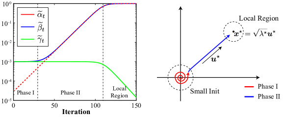
Figure 1: Evolution of the quantities $\widetilde{\alpha}_{t}$, $\widetilde{\beta}_{t}$, $\widetilde{\gamma}_{t}$ simulated with $\widetilde{\alpha}_{0}=\frac{1}{\sqrt{n}}\beta_{0}$, $\beta_{0}=\frac{1}{n}$, $\lambda^{\star}=1$, and $n=1000$. (right) Trajectory of $\widetilde{\bm{x}}^{(t)}$. It starts from a point that is close to the origin due to small initialization. It finds the direction $\bm{u}^{\star}$ while rotating around the origin, and once it finds the direction, it keeps the direction and gets expanded.

4 Fully Observed Case and Proof Sketch

Before we explain about the proof of Theorems 3.1 and 3.2, we describe the trajectory of fully observed case. We characterize $\widetilde{\bm{x}}^{(t)}$ with three variables: $\widetilde{\alpha}_{t}=\MT@delim@PAIRED\abs@star{\bm{u}^{\star\top}\widetilde{\bm{x}}^{(t)}}$, $\widetilde{\beta}_{t}=\lVert\widetilde{\bm{x}}^{(t)}\rVert_{2}$, $\widetilde{\gamma}_{t}=\lVert\widetilde{\bm{x}}_{\perp}^{(t)}\rVert_{2}$. According to Eq. 3, the three variables evolve with

$$\widetilde{\alpha}_{t+1} =(1-\eta\widetilde{\beta}_{t}^{2}+\eta\lambda^{\star})\widetilde{\alpha}_{t},$$

$$\widetilde{\gamma}_{t+1} =(1-\eta\widetilde{\beta}_{t}^{2})\widetilde{\gamma}_{t},$$

$$\widetilde{\beta}_{t}^{2} =\widetilde{\alpha}_{t}^{2}+\widetilde{\gamma}_{t}^{2}.$$

At $t=0$, due to random initialization, the initial vector is almost orthogonal to $\bm{u}^{\star}$, and we have $\widetilde{\alpha}_{0}\approx\frac{1}{\sqrt{n}}\beta_{0}$ and $\widetilde{\gamma}_{0}\approx\widetilde{\beta}_{0}=\beta_{0}$. Also, due to small initialization, the term $\eta\widetilde{\beta}_{t}^{2}$ is ignorable until $\widetilde{\beta}_{t}$ becomes sufficiently large, so $\widetilde{\alpha}_{t}$ increases exponentially with the rate $1+\eta\lambda^{\star}$ while $\widetilde{\gamma}_{t}$ stays still. Hence, at the early iterations where $(1+\eta\lambda^{\star})^{t}$ is still much less than $\sqrt{n}$, $\widetilde{\beta}_{t}$ is kept to its initial value $\beta_{0}$, while the trajectory becomes more parallel to $\bm{u}^{\star}$ because $\widetilde{\alpha}_{t}$ increases. When $(1+\eta\lambda^{\star})^{t}$ gets much larger than $\sqrt{n}$, the trajectory becomes almost parallel to $\bm{u}^{\star}$ in that $\widetilde{\beta}_{t}\approx\widetilde{\alpha}_{t}\gg\widetilde{\gamma}_{t}$. Until $\widetilde{\beta}_{t}$ (asymptotically) reaches $\frac{\sqrt{\lambda^{\star}}}{\sqrt{\log n}}$, we can consider $\widetilde{\alpha}_{t}$ as increasing in a rate $(1+\eta\lambda^{\star})$, and it takes about $\frac{1}{\log(1+\eta\lambda^{\star})}\log\frac{\sqrt{\lambda^{\star}n}}{\beta_{0}}$ steps to reach this point. After this, we can no longer ignore the term $\eta\widetilde{\beta}_{t}^{2}$, and $\widetilde{\alpha}_{t}$ increases with slower rate as $\widetilde{\beta}_{t}$ increases. We can show that $\widetilde{\beta}_{t}^{2}$ becomes sufficiently close to $\lambda^{\star}$ within $O(\log\log n)$ additional iterations as stated in the following lemma.

Lemma 4.1.

Let $T_{2}^{\prime}$ be the largest $t$ such that $\widetilde{\beta}_{t}^{2}\leq\frac{\lambda^{\star}}{64\log n}$. At $t=T_{2}^{\prime}+\frac{6\log\log n}{\log(1+\eta\lambda^{\star})}$, we have $\widetilde{\beta}_{t}^{2}\geq\lambda^{\star}\left(1-\frac{1}{\log n}\right)$.

Finally, local convergence to $\bm{u}^{\star}$ occurs in that $\widetilde{\alpha}_{t}$ approaches $\lambda^{\star}$ and $\widetilde{\gamma}_{t}$ decreases exponentially with the rate $(1-\eta\lambda^{\star})$. We plotted the actual behavior of quantities $\widetilde{\alpha}_{t}$, $\widetilde{\beta}_{t}$, $\widetilde{\gamma}_{t}$ on the left side of Fig. 1.

We define the iterates before $(1+\eta\lambda^{\star})^{t}$ reaches $\frac{1}{\sqrt{np}}\sqrt{n}$, within some logarithmic factors, as Phase I, and the next iterates before $\widetilde{\beta}_{t}^{2}$ reaches $\lambda^{\star}\left(1-\frac{1}{\log n}\right)$ as Phase II. Different techniques were used for each phase to prove that $\bm{x}^{(t)}$ stays close to $\widetilde{\bm{x}}^{(t)}$. At the end of Phase I, $\widetilde{\alpha}_{t}$ is increased to $\frac{1}{\sqrt{np}}\beta_{0}$ from its initial scale $\frac{1}{\sqrt{n}}\beta_{0}$, but still it is not dominant over $\beta_{0}$. Hence, the magnitudes of both $\bm{x}^{(t)}$ and $\widetilde{\bm{x}}^{(t)}$ are kept to $\beta_{0}$ throughout Phase I, and we take advantage of the small random initialization to show that the deviation of $\bm{x}^{(t)}$ from $\widetilde{\bm{x}}^{(t)}$ does not increase much and is kept to $\sqrt{\frac{1}{np}}$ times the norms of $\bm{x}^{(t)}$. In Phase II, we show that $\bm{x}^{(t)}-\widetilde{\bm{x}}^{(t)}$ expands at a rate at most $(1+\eta\lambda^{\star})$. Because the norms of $\bm{x}^{(t)}$ also increases at a rate $(1+\eta\lambda^{\star})$ during most of Phase II, the norms of $\bm{x}^{(t)}-\widetilde{\bm{x}}^{(t)}$ remain negligible compared to those of $\bm{x}^{(t)}$. The next two sections respectively give main lemmas of Phase I and II that will be used to prove Theorems 3.1 and 3.2.

5 Phase I: Finding Direction

We provide detailed results and proof ideas for Phase I in this section. Our main goal is to analyze the deviation of $\bm{x}^{(t)}$ from $\widetilde{\bm{x}}^{(t)}$. First, if we look at the update equations Eq. 2 and Eq. 3, the second term is proportional to the third power of $\left\lVert\bm{x}^{(t)}\right\rVert_{2}$, while the other terms linearly depend on $\left\lVert\bm{x}^{(t)}\right\rVert_{2}$. Hence, the second term becomes almost negligible due to small initialization. Without the second terms, the difference between $\bm{x}^{(t)}$ and $\widetilde{\bm{x}}^{(t)}$ at $t=1$ is $\eta(\bm{M}^{\circ}-\bm{M}^{\star})\bm{x}^{(0)}$. From concentration inequalities, one can show that the $\ell_{2}$ and $\ell_{\infty}$-norms of ${\bm{x}}^{(1)}-\widetilde{\bm{x}}^{(1)}$ are bounded by

$$\left\lVert{\bm{x}}^{(1)}-\widetilde{\bm{x}}^{(1)}\right\rVert_{2} \lesssim\mu\sqrt{\frac{\log n}{np}}\beta_{0},$$

$$\left\lVert{\bm{x}}^{(1)}-\widetilde{\bm{x}}^{(1)}\right\rVert_{\infty} \lesssim\mu\sqrt{\frac{\log^{2}n}{np}}\frac{\beta_{0}}{\sqrt{n}}.$$

Thus, the norms of $\bm{x}^{(t)}-\widetilde{\bm{x}}^{(t)}$ are about $\frac{1}{\sqrt{np}}$ times smaller than those of $\widetilde{\bm{x}}^{(t)}$ at $t=1$.

Due to the third terms of Eq. 2 and Eq. 3, the norms of $\bm{x}^{(t)}-\widetilde{\bm{x}}^{(t)}$ can increase exponentially at a rate $(1+\eta\lambda^{\star})$ in the worst case where $\bm{x}^{(t)}-\widetilde{\bm{x}}^{(t)}$ is parallel to $\bm{u}^{\star}$. In such a case, the norms of $\bm{x}^{(t)}-\widetilde{\bm{x}}^{(t)}$ would be larger than those of $\widetilde{\bm{x}}^{(t)}$ at the end of Phase I because those of $\widetilde{\bm{x}}^{(t)}$ remain still in Phase I. However, we overcome this issue by proving that the bounds increase at most polynomially with respect to $t$, and because $t$ is at most $O(\log n)$, the bounds remain $\frac{1}{\sqrt{np}}$ times smaller than the norms of $\widetilde{\bm{x}}^{(t)}$ up to logarithmic factors throughout Phase I.

Lemma 5.1.

Let $T_{1}$ be the largest $t$ such that $(1+\eta\lambda^{\star})^{t}\leq\sqrt{\frac{\mu^{4}\log^{21}n}{np}}\sqrt{n}$. Suppose that the conditions of Theorem 3.1 hold. Then, for all $t\leq T_{1}$, we have

$$\left\lVert\bm{x}^{(t)}-\widetilde{\bm{x}}^{(t)}\right\rVert_{2} \lesssim\mu\sqrt{\frac{\log n}{np}}\beta_{0}t,$$ (12)

$$\left\lVert\bm{x}^{(t)}-\widetilde{\bm{x}}^{(t)}\right\rVert_{\infty} \lesssim\sqrt{\frac{\mu^{3}\log^{2}n}{np}}\frac{\beta_{0}}{\sqrt{n}}t^{3}$$ (13)

with probability at least $1-o(1/\sqrt{\log n})$.

$T_{1}$ is defined to be the end of Phase I. Lemma 5.1 proves Theorem 3.2 for Phase I.

5.1 Proof of Eq. 12

We first demonstrate how to obtain the $\ell_{2}$-norm bound of Lemma 5.1. Let us define a sequence $\widehat{\bm{x}}^{(t)}$ that is updated with

$$\widehat{\bm{x}}^{(t+1)}=\widehat{\bm{x}}^{(t)}-\eta\left\lVert\widetilde{\bm{x}}^{(t)}\right\rVert_{2}^{2}\widehat{\bm{x}}^{(t)}+\eta\bm{M}^{\circ}\widehat{\bm{x}}^{(t)},\quad\widehat{\bm{x}}^{(0)}=\bm{x}^{(0)}.$$ (14)

Note that the norm of $\widetilde{\bm{x}}^{(t)}$ is used in the second term of Eq. 14. The update equation of $\widehat{\bm{x}}^{(t)}$ differs on the third term compared to $\widetilde{\bm{x}}^{(t)}$ and on the second term compared to $\bm{x}^{(t)}$. We use $\widehat{\bm{x}}^{(t)}$ as a proxy for bounding $\left\lVert\bm{x}^{(t)}-\widetilde{\bm{x}}^{(t)}\right\rVert_{2}$. We first show that $\left\lVert\widehat{\bm{x}}^{(t)}-\widetilde{\bm{x}}^{(t)}\right\rVert_{2}$ increases at most linearly with respect to $t$.

Lemma 5.2.

For all $t\leq T_{1}$, we have

$$\left\lVert\widehat{\bm{x}}^{(t)}-\widetilde{\bm{x}}^{(t)}\right\rVert_{2}\lesssim\mu\sqrt{\frac{\log n}{np}}\beta_{0}t$$ (15)

with probability at least $1-o(1/\sqrt{\log n})$.

The proof of this lemma is based on the fact that $\widehat{\bm{x}}^{(t)}$ is a product between $\bm{x}^{(0)}$ and a matrix polynomial of ${\bm{I}}$, $\bm{M}^{\circ}$, while $\widetilde{\bm{x}}^{(t)}$ is a product between $\bm{x}^{(0)}$ and a matrix polynomial of ${\bm{I}}$, $\bm{M}^{\star}$. We prove the lemma by comparing the two matrix polynomials. We remark that Lemma 5.2 holds regardless of the small initialization, but it relies on the randomness of $\bm{x}^{(0)}$.

Because $\bm{x}^{(t)}$ and $\widehat{\bm{x}}^{(t)}$ differ only on the second term, their initial difference is proportional to $\beta_{0}^{3}$. More precisely, it is $\frac{1}{\sqrt{np}}\beta_{0}^{3}$. We show that the difference increases exponentially at a rate $(1+\eta\lambda^{\star})$.

Lemma 5.3.

If Eq. 13 holds for all $t\leq T_{1}$, we have

$$\left\lVert\bm{x}^{(t)}-\widehat{\bm{x}}^{(t)}\right\rVert_{2}\lesssim\frac{1}{\lambda^{\star}}\sqrt{\frac{\mu^{3}\log^{3}n}{np}}(1+\eta\lambda^{\star})^{t}\beta_{0}^{3}t$$ (16)

for all $t\leq T_{1}$ with probability at least $1-o(1/\sqrt{\log n})$.

The upper bound in Eq. 16 becomes smaller than that of Eq. 15 when $(1+\eta\lambda^{\star})^{t}\beta_{0}^{2}\leq\lambda^{\star}\sqrt{\frac{1}{\mu\log^{2}n}}$. One can check that this condition is satisfied from the definition of $T_{1}$ given in Lemma 5.1 and the bound on initialization size Eq. 9. Hence, Eq. 12 is proved by Eq. 15 and Eq. 16.

5.2 Proof of Eq. 13

We control the $l$th component of $\bm{x}^{(t)}-\widetilde{\bm{x}}^{(t)}$ with the help of $l$th leave-one-out sequence. The leave-one-out sequences have two important properties. First, because they are defined without only one row/column, they are extremely close to $\bm{x}^{(t)}$, and at $t=1$, $\left\lVert\bm{x}^{(t)}-\bm{x}^{(t,l)}\right\rVert_{2}$ is about $\frac{1}{\sqrt{np}}\frac{1}{\sqrt{n}}$. Second, the $l$th component of the $l$th leave-one-out sequence evolves similar to that of $\widetilde{\bm{x}}^{(t)}$, and it is easy to analyze. With these two properties, we bound the $l$th component of $\bm{x}^{(t)}-\widetilde{\bm{x}}^{(t)}$ as

$$\MT@delim@PAIRED\abs@star{\left(\bm{x}^{(t)}-\widetilde{\bm{x}}^{(t)}\right)_{l}}\leq\left\lVert\bm{x}^{(t)}-\bm{x}^{(t,l)}\right\rVert_{2}+\MT@delim@PAIRED\abs@star{\left(\bm{x}^{(t,l)}-\widetilde{\bm{x}}^{(t)}\right)_{l}}.$$ (17)

We claim that both $\left\lVert\bm{x}^{(t)}-\bm{x}^{(t,l)}\right\rVert_{2}$ and $\MT@delim@PAIRED\abs@star{\left(\bm{x}^{(t,l)}-\widetilde{\bm{x}}^{(t)}\right)_{l}}$ increase at most polynomially with respect to $t$ from the initial scale $\frac{1}{\sqrt{np}}\frac{\beta_{0}}{\sqrt{n}}$.

Lemma 5.4.

For all $t\leq T_{1}$, we have

$$\left\lVert\bm{x}^{(t)}-\bm{x}^{(t,l)}\right\rVert_{2} \lesssim\mu\sqrt{\frac{\log^{2}n}{np}}\frac{\beta_{0}}{\sqrt{n}}t$$ (18)

$$\MT@delim@PAIRED\abs@star{\left(\bm{x}^{(t,l)}-\widetilde{\bm{x}}^{(t)}\right)_{l}} \lesssim\sqrt{\frac{\mu^{3}\log^{2}n}{np}}\frac{\beta_{0}}{\sqrt{n}}t^{3},$$ (19)

with probability at least $1-o(1/\sqrt{\log n})$.

As explained for $\bm{x}^{(t)}-\widetilde{\bm{x}}^{(t)}$, due to the third terms of Eq. 2 and Eq. 14, $\bm{x}^{(t)}-\bm{x}^{(t,l)}$ can also increase exponentially with the rate $(1+\eta\lambda^{\star})$ in the worst case where $\bm{x}^{(t)}-\bm{x}^{(t,l)}$ is parallel to $\bm{u}^{\star}$. This is contrary to our result Eq. 18 that $\left\lVert\bm{x}^{(t)}-\bm{x}^{(t,l)}\right\rVert_{2}$ increases only linearly. We show that $\bm{x}^{(t)}-\bm{x}^{(t,l)}$ is maintained almost orthogonal to $\bm{u}^{\star}$ in Phase I, and thus the worst case does not happen.

Lemma 5.5.

For all $l\in[n]$ and $t\leq T_{1}$, we have

$$\MT@delim@PAIRED\abs@star{\displaystyle\bm{u}^{(l)\top}(\bm{x}^{(t)}-\bm{x}^{(t,l)})}\lesssim\sqrt{\frac{\mu^{3}\log^{2}n}{np}}(1+\eta\lambda^{\star})^{t}\frac{\beta_{0}}{n}$$

with probability at least $1-o(1/\sqrt{\log n})$, where $\displaystyle\bm{u}^{(l)}$ is the first eigenvector of $\bm{M}^{(l)}$.

Note that $\displaystyle\bm{u}^{(l)}$ is almost parallel to $\bm{u}^{\star}$. The $\displaystyle\bm{u}^{(l)}$ component of $\bm{x}^{(t)}-\bm{x}^{(t,l)}$ is initialized at the order $\frac{1}{\sqrt{np}}\frac{\beta_{0}}{n}$, which is $\frac{1}{\sqrt{n}}$ times smaller than $\left\lVert\bm{x}^{(t)}-\bm{x}^{(t,l)}\right\rVert_{2}$. Although it is increased exponentially, from the definition of $T_{1}$, the $\displaystyle\bm{u}^{(l)}$ component is maintained much smaller than $\left\lVert\bm{x}^{(t)}-\bm{x}^{(t,l)}\right\rVert_{2}$ in Phase I.

One can show that $\MT@delim@PAIRED\abs@star{\left(\bm{x}^{(t,l)}-\widetilde{\bm{x}}^{(t)}\right)_{l}}$ increases by $\left\lVert\bm{x}^{(t)}-\widetilde{\bm{x}}^{(t)}\right\rVert_{2}\left\lVert\bm{u}^{\star}\right\rVert_{\infty}$ in each step, and summation of the bound Eq. 12 up to $t$ gives Eq. 19. Finally, Eq. 13 is obtained by putting Eq. 18 and Eq. 19 into Eq. 17.

6 Phase II: Expansion

In the next phase, we show that the bounds obtained in Phase I are increased at a rate $(1+\eta\lambda^{\star})$.

Lemma 6.1.

Let $T_{2}$ be the largest $t$ such that $\widetilde{\beta}_{t}^{2}\leq\lambda^{\star}\left(1-\frac{1}{\log n}\right)$. Then, for all $T_{1}<t\leq T_{2}$, we have

$$\left\lVert\bm{x}^{(t)}-\widetilde{\bm{x}}^{(t)}\right\rVert_{2}\lesssim\mu\sqrt{\frac{\log^{3}n}{np}}\beta_{0}(1+\eta\lambda^{\star})^{t-T_{1}},$$ (20)

$$\left\lVert\bm{x}^{(t)}-\widetilde{\bm{x}}^{(t)}\right\rVert_{\infty}\lesssim\sqrt{\frac{\mu^{3}\log^{8}n}{np}}\frac{\beta_{0}}{\sqrt{n}}(1+\eta\lambda^{\star})^{t-T_{1}},$$ (21)

$$\left\lVert\bm{x}^{(t)}-\bm{x}^{(t,l)}\right\rVert_{2}\lesssim\mu\sqrt{\frac{\log^{5}n}{np}}\frac{\beta_{0}}{\sqrt{n}}(1+\eta\lambda^{\star})^{t-T_{1}},$$ (22)

$$\MT@delim@PAIRED\abs@star{\left(\bm{x}^{(t,l)}-\widetilde{\bm{x}}^{(t)}\right)_{l}}\lesssim\sqrt{\frac{\mu^{3}\log^{8}n}{np}}\frac{\beta_{0}}{\sqrt{n}}(1+\eta\lambda^{\star})^{t-T_{1}},$$ (23)

with probability at least $1-o(1/\sqrt{\log n})$.

$T_{2}$ is defined to be the end of Phase II. We explain how Lemma 6.1 leads to Theorem 3.2 in Phase II. We first focus on Eq. 20 and Eq. 10. We can divide Phase II into three parts according to the behavior of $\left\lVert\widetilde{\bm{x}}^{(t)}\right\rVert_{2}$. First, $\left\lVert\widetilde{\bm{x}}^{(t)}\right\rVert_{2}$ is maintained to $\beta_{0}$ until $(1+\eta\lambda^{\star})^{t}$ becomes $\sqrt{n}$, or $(1+\eta\lambda^{\star})^{t-T_{1}}$ becomes $\sqrt{np}$. In this part, although the bounds increase exponentially with the rate $(1+\eta\lambda^{\star})$, $\frac{1}{\sqrt{np}}$ factor that was already present in Eq. 12 of Phase I compensates this increment. At the end of the first part, $\left\lVert\bm{x}^{(t)}-\widetilde{\bm{x}}^{(t)}\right\rVert_{2}$ is smaller than $\left\lVert\widetilde{\bm{x}}^{(t)}\right\rVert_{2}$ by some log factors. Next, $\left\lVert\widetilde{\bm{x}}^{(t)}\right\rVert_{2}$ increases with the rate $(1+\eta\lambda^{\star})$ until it reaches $\frac{\sqrt{\lambda^{\star}}}{8\sqrt{\log n}}$. Because both $\left\lVert\bm{x}^{(t)}-\widetilde{\bm{x}}^{(t)}\right\rVert_{2}$ and $\left\lVert\widetilde{\bm{x}}^{(t)}\right\rVert_{2}$ increase with $(1+\eta\lambda^{\star})$, the ratio between them is maintained in the second part. Lastly, in the remaining iterations, $\left\lVert\widetilde{\bm{x}}^{(t)}\right\rVert_{2}$ increases with $(1-\eta\widetilde{\beta}_{t}^{2}+\eta\lambda^{\star})$ at each step, and the increment becomes smaller as it converges to $\sqrt{\lambda^{\star}}$. Hence, as in the first part, $\left\lVert\bm{x}^{(t)}-\widetilde{\bm{x}}^{(t)}\right\rVert_{2}$ increases faster than $\left\lVert\widetilde{\bm{x}}^{(t)}\right\rVert_{2}$. However, from Lemma 4.1, the length of this part is $O(\log\log n)$, and the ratio between $\left\lVert\bm{x}^{(t)}-\widetilde{\bm{x}}^{(t)}\right\rVert_{2}$ and $\left\lVert\widetilde{\bm{x}}^{(t)}\right\rVert_{2}$ increases only by $\log^{6}n$. We prove that the log factors already present at the end of the second part compensates this, and finally Eq. 10 holds for all $t$ in Phase II. A more delicate analysis may prove that $\left\lVert\bm{x}^{(t)}-\widetilde{\bm{x}}^{(t)}\right\rVert_{2}$ increases with the same rate as $\left\lVert\widetilde{\bm{x}}^{(t)}\right\rVert_{2}$ in the thrid part, and it will reduce the required sample complexity by at most $\log^{12}n$. A similar argument can be used to prove that the bounds for $\left\lVert\bm{x}^{(t)}-\widetilde{\bm{x}}^{(t)}\right\rVert_{\infty}$, $\left\lVert\bm{x}^{(t)}-\bm{x}^{(t,l)}\right\rVert_{2}$, and $\MT@delim@PAIRED\abs@star{(\bm{x}^{(t,l)}-\widetilde{\bm{x}}^{(t)})_{l}}$ are less than $\left\lVert\widetilde{\bm{x}}^{(t)}\right\rVert_{\infty}$ by some log factors throughout Phase II.

At the end of Phase II, $\widetilde{\bm{x}}^{(t)}$ is very close to $\pm\bm{x}^{\star}$ in both $\ell_{2}$ and $\ell_{\infty}$-norms, so one can substitute $\widetilde{\bm{x}}^{(t)}$ of Lemma 6.1 with $\pm\bm{x}^{\star}$ to prove Eqs. 5 to 8 of Theorem 3.1. Hence, we can let $T^{\star}=T_{2}$, and as explained in Section 4, $T_{2}$ is approximately given by $\frac{1}{\log(1+\eta\lambda^{\star})}\log\frac{\sqrt{\lambda^{\star}n}}{\beta_{0}}+O(\log\log n)$, which is $(1+o(1))\frac{1}{\eta\lambda^{\star}}\log\frac{\sqrt{\lambda^{\star}n}}{\beta_{0}}$.

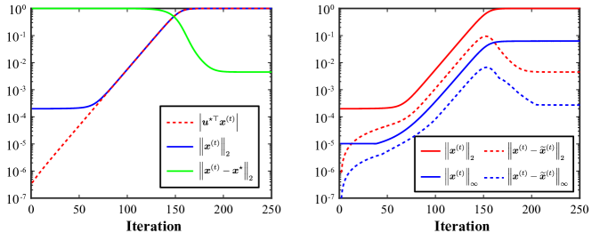
Figure 2: Trajectory of GD obtained with $n=5000$, $\lambda^{*}=1$, $p=0.1$, $\sigma=\frac{0.1}{n}$, $\beta_{0}=\frac{1}{n}$, $\eta=0.1$ for $\bm{u}^{\star}$ generated by normalizing a Gaussian vector. (left) Evolution of the quantities $|\bm{u}^{\star\top}\bm{x}^{(t)}|$, $\|\bm{x}^{(t)}\|_{2}$ that behaves similar to $\widetilde{\alpha}_{t}$, $\widetilde{\beta}_{t}$, respectively, and $\|\bm{x}^{(t)}\pm\bm{x}^{\star}\|_{2}$ that shows local convergence. (right) Comparison between the norms of $\bm{x}^{(t)}$ and $\bm{x}^{(t)}-\widetilde{\bm{x}}^{(t)}$.

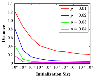
Figure 3: Convergence of GD with respect to initialization size and sampling probability. $\|\bm{x}^{(t)}\pm\bm{x}^{*}\|_{2}$ was measured at $t=\frac{1}{\log(1+\eta\lambda^{\star})}\log\frac{\sqrt{\lambda^{\star}n}}{\beta_{0}}+100$ and averaged over $1000$ trials. The conditions used in Fig. 2 were used again, but with $n=500$.

7 Simulation

In this section, we provide some simulation results that support our theoretical findings.

Trajectory of GD

With the dimension $n=5000$, we constructed the ground truth vector $\bm{u}^{\star}$ by sampling it from the Gaussian distribution $\mathcal{N}(\bm{0},\frac{1}{n}{\bm{I}})$ and normalized it to have unit norm. We let $\lambda^{\star}=1$ so that the matrix $\bm{M}^{\star}$ is given by $\bm{u}^{\star}\bm{u}^{\star\top}$, and we randomly sampled the matrix symmetrically with sampling rate $p=0.1$ and Gaussian noise of $\sigma=\frac{0.1}{n}$. The initialization size was set to $\beta_{0}=\frac{1}{n}$ and step size of $0.1$ was used for GD. Fig. 2 represents one trial of the experiment, but similar graphs were obtained in every repetition of the experiment. The evolution of some important quantities such as $\left\lVert\bm{x}^{(t)}\right\rVert_{2}$ and $\MT@delim@PAIRED\abs@star{\bm{u}^{\star\top}\bm{x}^{(t)}}$ are depicted on the left side of Fig. 2. As observed in the fully observed case, the signal component $\MT@delim@PAIRED\abs@star{\bm{u}^{\star\top}\bm{x}^{(0)}}$ increases with the rate $(1+\eta\lambda^{\star})$ until it gets close to $\sqrt{\lambda^{\star}}$, and local convergence to $\bm{x}^{\star}$ occurs, where $\left\lVert\bm{x}^{(t)}-\bm{x}^{\star}\right\rVert_{2}$ decreases exponentially and saturates at the level determined by noise size $\sigma$. On the right side of Fig. 2, we describe the deviation of $\bm{x}^{(t)}$ from $\widetilde{\bm{x}}^{(t)}$ in both $\ell_{2}$ and $\ell_{\infty}$-norms. The solid lines represent norms of $\bm{x}^{(t)}$ and the dotted lines represent those of $\bm{x}^{(t)}-\widetilde{\bm{x}}^{(t)}$. We could observe that there is a gap between solid and dotted lines throughout whole iterations. Hence, $\bm{x}^{(t)}$ stays close to the trajectory of fully observed case as we proved in Theorem 3.2.

Small Initialization

In the next experiment, we assessed the importance of small initialization for convergence of GD. We used the same conditions used in the previous experiment except $n=500$. We measured $\left\lVert\bm{x}^{(t)}\pm\bm{x}^{\star}\right\rVert_{2}$ at $t=\frac{1}{\log(1+\eta\lambda^{\star})}\log\frac{\sqrt{\lambda^{\star}n}}{\beta_{0}}+100$ and averaged it over $1000$ trials. We repeated the experiment while changing the initialization size from $10^{0}$ to $10^{-9}$ and the sampling probability from $0.01$ to $0.04$. The result is summarized to Fig. 3. In all sampling probabilities, the small initialization improves the convergence of GD. Also, the performance starts to saturate at much larger initialization size as sampling probability increases, and this agrees with our finding Eq. 9 that a larger initialization is possible as more samples are available.

8 Discussion

In this paper, we showed that for rank-1 symmetric matrix completion with $\ell_{2}$-loss, GD can converge to the ground truth starting from a small random initialization. Ignoring for logarithmic factors, the bound on initialization size reads $n^{-\frac{1}{4}}$ when optimal number of samples are provided, and the bound becomes larger as more samples are provided. The result is interesting because the loss function does not have global benign geometry if no regularizer is applied. Our result does not use any explicit regularizer and only rely on the implicit regularizing effect of GD.

The most important future work is an extension to the rank-$r$ case. Suppose that $\bm{M}^{\star}$ is a rank-$r$ matrix and its eigendecomposition is given by $\bm{U}^{\star}\bm{\Sigma}^{\star}\bm{U}^{\star\top}=\bm{X}^{\star}\bm{X}^{\star\top}$, where $\bm{\Sigma}^{\star}=\operatorname{diag}(\lambda_{1}^{\star},\cdots,\lambda_{r}^{\star})$ and $\bm{X}^{\star}=\bm{U}^{\star}\bm{\Sigma}^{\star\frac{1}{2}}$. Then, the trajectory of GD becomes an $n\times r$ matrix $\bm{X}^{(t)}$, which is updated with

$$\bm{X}^{(t+1)}=\bm{X}^{(t)}-\frac{\eta}{p}\mathcal{P}_{#1}\left(\bm{X}^{(t)}\bm{X}^{(t)\top}\right)\bm{X}^{(t)}+\eta\bm{M}^{\circ}\bm{X}^{(t)}.$$

Each entry of $\bm{X}^{(0)}$ is sampled independently from the Gaussian distribution $\mathcal{N}\left(0,\frac{1}{n}\beta_{0}^{2}\right)$ as in the rank-1 case.

One instance of $\bm{X}^{(t)}$ is depicted in Fig. 4. The same conditions as in Fig. 3 are used, except that the ground truth matrix is a rank-3 matrix with nonzero eigenvalues $1,0.75,0.5$. The singular values of $\bm{X}^{(t)}$ behave similar to $\left\lVert\bm{x}^{(t)}\right\rVert_{2}$ of the rank-1 case. At the early iterations where orthogonal components dominate, the singular values stay near their initial scale $\beta_{0}$. After that, each singular value $\sigma_{i}(\bm{X}^{(t)})$ increases at a rate $(1+\eta\lambda_{i}^{\star})$ and saturates at $\sqrt{\lambda_{i}^{\star}}$. We use $\left\lVert{\bm{X}}-{\bm{Y}}\right\rVert_{\mathrm{R}}$ to denote the Frobenius norm between ${\bm{X}}$ and ${\bm{Y}}$ under best rotational alignment. $\left\lVert\bm{X}^{(t)}-\bm{X}^{\star}\right\rVert_{\mathrm{R}}$ decreases exponentially and saturates at the level determined by noise size $\sigma$, after all singular values saturate, as local convergence begins.

In order to extend the results of rank-1 case, we need to show that $\left\lVert\bm{X}^{(t)}-\smash{\widetilde{\bm{X}}^{(t)}}\right\rVert_{\mathrm{R}}$ stays much less than $\left\lVert\bm{X}^{(t)}\right\rVert_{\mathrm{F}}$ throughout the iterations. Before $\sigma_{1}(\bm{X}^{(t)})$ saturates around $\sqrt{\lambda_{1}^{\star}}$, it behaves similar to $\left\lVert\bm{x}^{(t)}-\widetilde{\bm{x}}^{(t)}\right\rVert_{2}$ of the rank-1 case, i.e. it expands at a rate $(1+\eta\lambda_{1}^{\star})$ together with $\left\lVert\bm{X}^{(t)}\right\rVert_{\mathrm{F}}$ after the early iterations. However, because each singular value increases at a different rate, different phenomenon is observed for the rank-$r$ case. During the iterations before $\sigma_{i+1}(\bm{X}^{(t)})$ saturates after $\sigma_{i}(\bm{X}^{(t)})$ does, both $\left\lVert\bm{X}^{(t)}-\smash{\widetilde{\bm{X}}^{(t)}}\right\rVert_{\mathrm{R}}$ and $\left\lVert\bm{X}^{(t)}\right\rVert_{\mathrm{F}}$ do not increase much. Our current theory can only show that $\left\lVert\bm{X}^{(t)}-\smash{\widetilde{\bm{X}}^{(t)}}\right\rVert_{\mathrm{R}}$ increases at a rate less than $(1+\eta\lambda_{i+1}^{\star})$, and in order for $\left\lVert\bm{X}^{(t)}-\smash{\widetilde{\bm{X}}^{(t)}}\right\rVert_{\mathrm{R}}$ to stay much less than $\left\lVert\bm{X}^{(t)}\right\rVert_{\mathrm{F}}$, extra sample complexity is required to compensate for the exponential increases. Hence, we expect that the convergence of GD for rank-$r$ case can be proved with the techniques developed in this paper if $n^{1+\Theta(\kappa-1)}\operatorname{poly}(\kappa,r,\log n)$ samples are provided, where $\kappa=\frac{\lambda_{1}^{\star}}{\lambda_{r}^{\star}}$ is the condition number. Nevertheless, whether GD can converge with the optimal $n\operatorname{poly}(\kappa,r,\log n)$ samples for rank-$r$ matrix completion problem is left as an open problem.

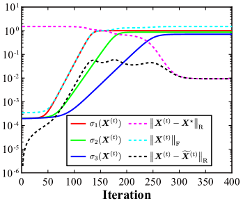
Figure 4: Trajectory of GD obtained for a rank-3 matrix with nonzero eigenvalues $1,0.75,0.5$. The same parameters used in Fig. 2 were used.

Detailed proofs for the results explained in the main text are provided in this supplementary. We say that an event happens with high probability if it happens with probability at least $1-\frac{1}{n^{C}}$ for a constant $C>0$ and $C$ can be made arbitrary large by controlling constant factors. A union of $\operatorname{poly}(n)$ number of events that happens with high probability still happens with high probability. For a matrix ${\bm{A}}$, we denote the spectral norm by $\MT@delim@PAIRED\norm@star{{\bm{A}}}$ and the maximum absolute value of entries by $\left\lVert{\bm{A}}\right\rVert_{\infty}$. Also, the largest $\ell_{2}$-norm of rows of ${\bm{A}}$ is denoted as $\left\lVert{\bm{A}}\right\rVert_{2,\infty}$.

Appendix A Spectral Analysis

We introduce some spectral bounds related to sampling and Gaussian noise.

Lemma A.1.

If $n^{2}p\gtrsim n\log n$, we have

$$\MT@delim@PAIRED\norm@star{\frac{1}{p}\mathcal{P}_{#1}\left(\bm{M}^{\star}\right)-\bm{M}^{\star}}\lesssim\lambda^{\star}\mu\sqrt{\frac{\log n}{np}}$$

with high probability.

Lemma A.2.

If $n^{2}p\gtrsim\mu n\log n$, for all $l\in[n]$, we have

$$\MT@delim@PAIRED\norm@star{\frac{1}{p}\mathcal{P}_{#1}\left(\bm{M}^{\star}\right)-\mathcal{P}^{(l)}_{#1}\left(\bm{M}^{\star}\right)}\lesssim\lambda^{\star}\sqrt{\frac{\mu}{np}}$$

with high probability.

Lemma A.3.

If $n^{2}p\gtrsim n\log^{2}n$, we have

$$\MT@delim@PAIRED\norm@star{\frac{1}{p}\mathcal{P}_{#1}\left({\bm{E}}\right)}\lesssim\sigma\sqrt{\frac{n}{p}}$$

with high probability.

Note that Lemma A.3 also implies that $\MT@delim@PAIRED\norm@star{\bm{E}^{(l)}}\lesssim\sigma\sqrt{\frac{n}{p}}$ for all $l\in[n]$ with high probability. Combined with the condition $\sigma\lesssim\frac{\lambda^{\star}\mu}{n}\sqrt{\log n}$, we have

$$\MT@delim@PAIRED\norm@star{\frac{1}{p}\mathcal{P}_{#1}\left({\bm{E}}\right)}\lesssim\lambda^{\star}\mu\sqrt{\frac{\log n}{np}},\quad\MT@delim@PAIRED\norm@star{\bm{E}^{(l)}}\lesssim\lambda^{\star}\mu\sqrt{\frac{\log n}{np}}$$

for all $l\in[n]$. Proofs for Lemmas A.1 and A.2 are provided in Appendix F, and see Lemma 11 of [11] for the proof of Lemma A.3.

Next, we state bounds on the eigenvalues of $\bm{M}^{\circ}$ and $\bm{M}^{(l)}$. The first eigenvalues of $\bm{M}^{\circ}$ and $\bm{M}^{(l)}$ are denoted as $\lambda^{\circ}$ and $\lambda^{(l)}$, respectively. The following lemma is derived from Lemmas A.1 and A.2 with Weyl’s Theorem.

Lemma A.4.

If $n^{2}p\gtrsim\mu n\log n$, we have

$$\MT@delim@PAIRED\abs@star{\lambda^{\circ}-\lambda^{\star}} \lesssim\lambda^{\star}\mu\sqrt{\frac{\log n}{np}}$$ (24)

$$\MT@delim@PAIRED\abs@star{\lambda^{(l)}-\lambda^{\star}} \lesssim\lambda^{\star}\mu\sqrt{\frac{\log n}{np}}$$ (25)

for all $l\in[n]$ with high probability.

Lastly, Lemmas A.1 and A.2 with Davis-Kahan Theorem gives the following lemma.

Lemma A.5.

If $n^{2}p\gtrsim\mu n\log n$, we have

$$\left\lVert\displaystyle\bm{u}^{(l)}-\bm{u}^{\star}\right\rVert_{2}\lesssim\mu\sqrt{\frac{\log n}{np}}$$

for all $l\in[n]$ with high probability.

Appendix B Initialization

We introduce some properties that the initialization vector $\bm{x}^{(0)}$ satisfies in this section. Recall that each entry of $\bm{x}^{(0)}$ is sampled from $\mathcal{N}(0,\frac{1}{n}\beta_{0}^{2})$ independently. We use ${\bm{H}}$ to denote the perturbation $\bm{M}^{\circ}-\bm{M}^{\star}$.

Lemma B.1.

The initialization vector $\bm{x}^{(0)}$ satisfies

$$\frac{1}{2}\beta_{0}\leq\left\lVert\bm{x}^{(0)}\right\rVert_{2}\leq\frac{3}{2}\beta_{0}$$ (26)

with probability at least $1-e^{-n/32}$, and

$$\left\lVert\bm{x}^{(0)}\right\rVert_{\infty}\leq 2\sqrt{\log n}\frac{\beta_{0}}{\sqrt{n}},$$ (27)

$$\MT@delim@PAIRED\abs@star{\bm{u}^{\star\top}{\bm{H}}^{s}\bm{x}^{(0)}}\leq 2\sqrt{\log n}\frac{\beta_{0}}{\sqrt{n}}\MT@delim@PAIRED\norm@star{{\bm{H}}}^{s},\quad\forall s\leq 30\log n,$$ (28)

with probability at least $1-\frac{1}{n}-\frac{30\log n}{n^{2}}$. It also satisfies

$$\frac{1}{\sqrt{\log n}}\frac{\beta_{0}}{\sqrt{n}}\leq\MT@delim@PAIRED\abs@star{\bm{u}^{\star\top}\bm{x}^{(0)}}$$ (29)

with probability at least $1-\frac{1}{2\sqrt{\log n}}$.

Proof.

To bound $\left\lVert\bm{x}^{(0)}\right\rVert_{2}$, we use the following basic concentration inequality that holds for i.i.d. standard normal variables $\{X_{i}\}_{i\in[n]}$.

$$\operatorname*{\mathbb{P}}\left[\MT@delim@PAIRED\abs@star{\frac{1}{n}\sum_{i=1}^{n}X_{i}^{2}-1}\geq t\right]\leq 2e^{-nt^{2}/8}$$

If we put $t=\frac{1}{2}$, with probability at least $1-e^{-n/32}$, we have

$$\frac{1}{2}\beta_{0}^{2}\leq\left\lVert\bm{x}^{(0)}\right\rVert_{2}^{2}\leq\frac{3}{2}\beta_{0}^{2},$$

and this implies Eq. 26.

For a centered Gaussian random variable with standard deviation $\sigma$, we have

$$\operatorname*{\mathbb{P}}\left[\MT@delim@PAIRED\abs@star{X}\geq t\right]\leq e^{-\frac{t^{2}}{2\sigma^{2}}}.$$

Hence, an entry of $\bm{x}^{(0)}$ is less than $2\sqrt{\log n}\frac{\beta_{0}}{\sqrt{n}}$ with probability at least $1-\frac{1}{n^{2}}$, and all entries of $\bm{x}^{(0)}$ is less than $2\sqrt{\log n}\frac{\beta_{0}}{\sqrt{n}}$ with probability at least $1-\frac{1}{n}$. $\bm{u}^{\star\top}{\bm{H}}^{s}\bm{x}^{(0)}$ follows a centered Gaussian distribution with standard deviation $\left\lVert{\bm{H}}^{s}\bm{u}^{\star}\right\rVert_{2}\leq\MT@delim@PAIRED\norm@star{{\bm{H}}}^{s}\left\lVert\bm{u}^{\star}\right\rVert_{2}$ for all $s$, and Eq. 28 holds with probability at least $1-\frac{10\log n}{n^{2}}$.

For a random variable $X$ that is sampled from $\mathcal{N}(0,\sigma^{2})$, we have

$$\operatorname*{\mathbb{P}}\left[\MT@delim@PAIRED\abs@star{X}\leq t\right]\leq\frac{t}{\sqrt{2\pi\sigma^{2}}}.$$

Hence, we have

$$\frac{1}{\sqrt{\log n}}\frac{\beta_{0}}{\sqrt{n}}\leq\MT@delim@PAIRED\abs@star{\bm{u}^{\star\top}\bm{x}^{(0)}}$$

with probability at least $1-\frac{1}{2\sqrt{\log n}}$. ∎

Lemma B.1 implies that the $\bm{u}^{\star}$ component of $\bm{x}^{(0)}$ is in the range

$$\frac{1}{\sqrt{\log n}}\frac{\beta_{0}}{\sqrt{n}}\leq\MT@delim@PAIRED\abs@star{\bm{u}^{\star\top}\bm{x}^{(0)}}\leq 2\sqrt{\log n}\frac{\beta_{0}}{\sqrt{n}}.$$ (30)

Lemma B.2.

We have

$$\left\lVert a\bm{x}^{(0)}+b\bm{u}^{\star}\right\rVert_{\infty}\geq(\MT@delim@PAIRED\abs@star{a}\beta_{0}+\MT@delim@PAIRED\abs@star{b})\frac{1}{\sqrt{n}}$$ (31)

for all $a,b$, with probability at least $1-\mathrm{exp}\left(-\frac{n}{2\mu}\right)$.

Proof.

The probability that an entry of $\bm{x}^{(0)}$ is less than $\frac{\beta_{0}}{\sqrt{n}}$ is bounded by $\frac{1}{\sqrt{2\pi}}$. Without loss of generality, let us assume that all entries of $\bm{u}^{\star}$ are not negative and $a,b\geq 0$. There are at least $\frac{n}{\mu}$ entries of $\bm{u}^{\star}$ that are larger than $\frac{1}{\sqrt{n}}$. For such entries, the probability that all entries of $\bm{x}^{(0)}$ is less than $\frac{\beta_{0}}{\sqrt{n}}$ is bounded by $\left(\frac{1}{\sqrt{2\pi}}\right)^{\frac{n}{\mu}}\leq\mathrm{exp}\left(-\frac{n}{2\mu}\right)$. Hence, for at least one position, both entries of $\bm{x}^{(0)}$ and $\bm{u}^{\star}$ are larger than $\frac{\beta_{0}}{\sqrt{n}}$ and $\frac{1}{\sqrt{n}}$, respectively, with probability at least $1-\mathrm{exp}\left(-\frac{n}{2\mu}\right)$. ∎

In the following sections, we assume that we are given an initialization vector $\bm{x}^{(0)}$ that satisfies Eqs. 26 to 31.

Appendix C Fully Observed Case

We provide some lemmas related to $\widetilde{\bm{x}}^{(t)}$ in this section. We first note that $\widetilde{\bm{x}}^{(t)}$ is explicitly written as

$$\widetilde{\bm{x}}^{(t)}=\prod_{s=1}^{t}(1-\eta\widetilde{\beta}_{s}^{2})\bm{x}^{(0)}+\prod_{s=1}^{t}(1-\eta\widetilde{\beta}_{s}^{2}+\eta\lambda^{\star})(\bm{u}^{\star\top}\bm{x}^{(0)})\bm{u}^{\star}:=A^{(t)}\bm{x}^{(0)}+B^{(t)}\bm{u}^{\star}.$$ (32)

Let us define $T_{2}^{\prime}$ as the last $t$ such that $\widetilde{\beta}_{t}^{2}\leq\frac{\lambda^{\star}}{64\log n}$. We claim that $T_{2}^{\prime}\leq\frac{64\log n}{\eta\lambda^{\star}}$ and prove this later. Then, for all $t\leq T_{2}^{\prime}$, we have

$$\begin{gathered}\frac{1}{4}(1+\eta\lambda^{\star})^{t}\leq\prod_{s=1}^{t}(1-\eta\widetilde{\beta}_{s}^{2}+\eta\lambda^{\star})\leq(1+\eta\lambda^{\star})^{t}\\ \frac{1}{4}\leq\prod_{s=1}^{t}(1-\eta\widetilde{\beta}_{s}^{2})\leq 1\end{gathered}$$ (33)

because

$$\prod_{s=1}^{T_{2}^{\prime}}\left(\frac{1+\eta\lambda^{\star}-\eta\widetilde{\beta}_{s}^{2}}{1+\eta\lambda^{\star}}\right)\geq\prod_{s=1}^{T_{2}^{\prime}}(1-\eta\widetilde{\beta}_{s}^{2})\geq\left(1-\frac{\eta\lambda^{\star}}{64\log n}\right)^{\frac{64\log n}{\eta\lambda^{\star}}}\geq\frac{1}{4}$$

if $\frac{\eta\lambda^{\star}}{64\log n}\leq\frac{1}{2}$. Note that the upper bounds in Eq. 33 hold even if $t>T_{2}$.

From Eq. 33, we have the approximation $\widetilde{\bm{x}}^{(t)}\approx\bm{x}^{(0)}+(1+\eta\lambda^{\star})^{t}(\bm{u}^{\star\top}\bm{x}^{(0)})\bm{u}^{\star}$ for all $t\leq T_{2}^{\prime}$ and the $\ell_{2}$-norm of $\widetilde{\bm{x}}^{(t)}$ is also approximately given by $\left(1+\frac{(1+\eta\lambda^{\star})^{t}}{\sqrt{n}}\right)\beta_{0}$. The $\ell_{\infty}$-norm is about $\frac{1}{\sqrt{n}}$ times smaller than the $\ell_{2}$-norm. We make this observation rigorous with the following lemma.

Lemma C.1.

For all $t\leq T_{2}^{\prime}$, we have

$$\frac{1}{8}\frac{1}{\sqrt{\log n}}\left(1+\frac{(1+\eta\lambda^{\star})^{t}}{\sqrt{n}}\right)\beta_{0} \leq\left\lVert\widetilde{\bm{x}}^{(t)}\right\rVert_{2}\leq 2\sqrt{\log n}\left(1+\frac{(1+\eta\lambda^{\star})^{t}}{\sqrt{n}}\right)\beta_{0},$$

$$\frac{1}{4}\frac{1}{\sqrt{\log n}}\left(1+\frac{(1+\eta\lambda^{\star})^{t}}{\sqrt{n}}\right)\frac{\beta_{0}}{\sqrt{n}} \leq\left\lVert\widetilde{\bm{x}}^{(t)}\right\rVert_{\infty}\leq 2\sqrt{\log n}\left(1+(1+\eta\lambda^{\star})^{t}\sqrt{\frac{\mu}{n}}\right)\frac{\beta_{0}}{\sqrt{n}}.$$

Proof.

For brevity, les us drop the superscript $(t)$ and write $\widetilde{\bm{x}}=A\bm{x}^{(0)}+B\bm{u}^{\star}$. For the upper bounds, we may use the triangle inequality

$$\MT@delim@PAIRED\norm@star{A\bm{x}^{(0)}+B\bm{u}^{\star}}\leq A\MT@delim@PAIRED\norm@star{\bm{x}^{(0)}}+\MT@delim@PAIRED\abs@star{B}\MT@delim@PAIRED\norm@star{\bm{u}^{\star}}.$$

If we use Eq. 30 and Eq. 33, we get the upper bounds for $A$ and $B$. We have $\left\lVert\bm{x}^{(0)}\right\rVert_{2}\leq 2\beta_{0}$ by Eq. 26, and the $\ell_{\infty}$-norm of $\bm{x}^{(0)}$ is controlled through Eq. 27. These finish the proof for the upper bounds.

From the definition of $B$, we have $B(\bm{u}^{\star\top}\bm{x}^{(0)})\geq 0$, and

$$\left\lVert A\bm{x}^{(0)}+B\bm{u}^{\star}\right\rVert_{2}^{2} =A^{2}\left\lVert\bm{x}^{(0)}\right\rVert_{2}^{2}+B^{2}+2AB(\bm{u}^{\star\top}\bm{x}^{(0)})$$

$$\geq A^{2}\left\lVert\bm{x}^{(0)}\right\rVert_{2}^{2}+B^{2}$$

$$\geq\frac{1}{4}\left(A\left\lVert\bm{x}^{(0)}\right\rVert_{2}+\MT@delim@PAIRED\abs@star{B}\right)^{2}.$$

Eq. 26 and Eq. 29 together with the lower bound in Eq. 33 gives the desired lower bound for $\left\lVert\widetilde{\bm{x}}\right\rVert_{2}$. The lower bound for $\ell_{\infty}$-norm is directly implied from Lemma B.2 together with Eq. 29 and Eq. 33. ∎

With Lemma C.1, we have

$$\frac{1}{8}\frac{1}{\sqrt{\log n}}\frac{(1+\eta\lambda^{\star})^{T_{2}^{\prime}}}{\sqrt{n}}\beta_{0}\leq\frac{1}{8}\frac{1}{\sqrt{\log n}}\left(1+\frac{(1+\eta\lambda^{\star})^{T_{2}^{\prime}}}{\sqrt{n}}\right)\beta_{0}\leq\left\lVert\widetilde{\bm{x}}^{(T_{2}^{\prime})}\right\rVert_{2}\leq\frac{\sqrt{\lambda^{\star}}}{8\sqrt{\log n}},$$

and thus

$$T_{2}^{\prime}\leq\frac{1}{\log(1+\eta\lambda^{\star})}\log\frac{\sqrt{\lambda^{\star}n}}{\beta_{0}}\leq\frac{11\log n}{\log(1+\eta\lambda^{\star})}\leq\frac{64\log n}{\eta\lambda^{\star}}.$$

For $t\leq T_{1}$ where $(1+\eta\lambda^{\star})^{t}$ is not big, the bounds in Lemma C.1 are simplified to

$$\frac{1}{\sqrt{\log n}}\beta_{0}\lesssim\left\lVert\widetilde{\bm{x}}^{(t)}\right\rVert_{2}\lesssim\sqrt{\log n}\beta_{0},$$ (34)

$$\frac{1}{\sqrt{\log n}}\frac{\beta_{0}}{\sqrt{n}}\lesssim\left\lVert\widetilde{\bm{x}}^{(t)}\right\rVert_{\infty}\lesssim\sqrt{\log n}\frac{\beta_{0}}{\sqrt{n}}.$$ (35)

After $\widetilde{\bm{x}}^{(t)}$ becomes almost parallel to $\bm{u}^{\star}$ and before $T_{2}^{\prime}$, we could approximate $\widetilde{\beta}_{t}$ as increasing with the rate $(1+\eta\lambda^{\star})$. However, after $T_{2}^{\prime}$, this approximation is invalid, and $\widetilde{\beta}_{t}$ grows at a slower rate as it increases and it eventually converges to $\sqrt{\lambda^{\star}}$. How much iterations will be required for it to reach $\sqrt{\lambda^{\star}}\sqrt{1-\frac{1}{\log n}}$ after $T_{2}^{\prime}$? With Lemma C.2, we will prove that $O(\log\log n)$ iterations are required after $T_{2}^{\prime}$.

Lemma C.2.

At $t=T_{2}^{\prime}+\frac{6\log\log n}{\log(1+\eta\lambda^{\star})}$, we have $\widetilde{\beta}_{t}^{2}\geq\lambda^{\star}\left(1-\frac{1}{\log n}\right)$.

Proof.

From the decomposition Eq. 32, we have

$$\MT@delim@PAIRED\abs@star{\left\lVert\widetilde{\bm{x}}^{(t)}\right\rVert_{2}-\MT@delim@PAIRED\abs@star{B^{(t)}}} \leq\left\lVert\bm{x}^{(0)}\right\rVert_{2}$$

$$\MT@delim@PAIRED\abs@star{\MT@delim@PAIRED\abs@star{\bm{u}^{\star\top}\bm{x}^{(0)}}-\MT@delim@PAIRED\abs@star{B^{(t)}}} \leq\MT@delim@PAIRED\abs@star{A^{(t)}}\MT@delim@PAIRED\abs@star{\bm{u}^{\star\top}\bm{x}^{(0)}}\leq\left\lVert\bm{x}^{(0)}\right\rVert_{2},$$

and thus

$$\MT@delim@PAIRED\abs@star{\widetilde{\alpha}_{t}-\widetilde{\beta}_{t}}\leq 2\left\lVert\bm{x}^{(0)}\right\rVert_{2}\leq\frac{\sqrt{\lambda^{\star}}}{3\log^{2}n}.$$ (36)

holds for all $t$. Because $\widetilde{\beta}_{t}\gtrsim\frac{1}{\log n}$ for all $t\geq T_{2}^{\prime}$, Eq. 36 implies that $\widetilde{\beta}_{t}$ is well approximated by $\widetilde{\alpha}_{t}$. Hence, we will focus on $\widetilde{\alpha}_{t}$, which is an increasing sequence that evolves with

$$\widetilde{\alpha}_{t+1}=(1-\eta\widetilde{\beta}_{t}^{2}+\eta\lambda^{\star})\widetilde{\alpha}_{t}.$$

For all $i\geq 1$, let $N_{i}$ be the last $t$ such that $\lambda^{\star}-\widetilde{\alpha}_{t}^{2}\geq\frac{\lambda^{\star}}{e^{i}}$. Then, we have

$$\lambda^{\star}-\widetilde{\alpha}_{N_{i}}^{2}\geq\frac{\lambda^{\star}}{e^{i}}>\lambda^{\star}-\widetilde{\alpha}_{N_{i}+1}^{2}.$$ (37)

Let $i\geq 2$. For all $N_{i-1}<t\leq N_{i}$,

$$\frac{\widetilde{\alpha}_{t+1}}{\widetilde{\alpha}_{t}}=1-\eta\widetilde{\beta}_{t}^{2}+\eta\lambda^{\star}=1+\eta(\lambda^{\star}-\widetilde{\alpha}_{t}^{2})+\eta(\widetilde{\alpha}_{t}^{2}-\widetilde{\beta}_{t}^{2})\geq 1+\frac{\eta\lambda^{\star}}{e^{i}}-\frac{\eta\lambda^{\star}}{\log^{2}n}\geq 1+0.99\frac{\eta\lambda^{\star}}{e^{i}}.$$

We used Eq. 36, Eq. 37, and the fact that $\widetilde{\alpha}_{t},\widetilde{\beta}_{t}\leq\sqrt{\lambda^{\star}}$ for all $t$. This implies

$$\left(1+0.99\frac{\eta\lambda^{\star}}{e^{i}}\right)^{N_{i}-N_{i-1}-1}x_{N_{i-1}+1}\leq x_{N_{i}}.$$

From the lower and upper bounds provided by Eq. 37, we have

$$\sqrt{\lambda^{\star}}\sqrt{1-\frac{1}{e^{i-1}}}\left(1+0.99\frac{\eta\lambda^{\star}}{e^{i}}\right)^{N_{i}-N_{i-1}-1}\leq\sqrt{\lambda^{\star}}\sqrt{1-\frac{1}{e^{i}}},$$

$$\left(1+0.99\frac{\eta\lambda^{\star}}{e^{i}}\right)^{2(N_{i}-N_{i-1}-1)}\leq\frac{e^{i}-1}{e^{i}}\frac{e^{i-1}}{e^{i-1}-1}=\frac{e^{i-1}-\frac{1}{e}}{e^{i-1}-1}\leq 1+\frac{1}{e^{i-1}}.$$

Taking $\log$ on both sides and using the inequality $\frac{1}{2}x<\log(1+x)<x$ that holds for $0<x<1$, we get

$$N_{i}-N_{i-1}\leq 1+\frac{1}{2}\frac{\log\left(1+\frac{1}{e^{i-1}}\right)}{\log\left(1+0.99\frac{\eta\lambda^{\star}}{e^{i}}\right)}\leq 1+\frac{e}{0.99\eta\lambda^{\star}}.$$

For $t\leq N_{1}$, we have

$$\frac{\widetilde{\alpha}_{t+1}}{\widetilde{\alpha}_{t}}\geq 1+0.99\frac{\eta\lambda^{\star}}{e},$$

and thus

$$\sqrt{\lambda^{\star}}\sqrt{1-\frac{1}{e}}\geq\alpha_{N_{1}}\geq\left(1+0.99\frac{\eta\lambda^{\star}}{e}\right)^{N_{1}}\widetilde{\alpha}_{T_{2}^{\prime}}=\left(1+0.99\frac{\eta\lambda^{\star}}{e}\right)^{N_{1}}\sqrt{\frac{\lambda^{\star}}{21\log n}}.$$

Taking $\log$ on both sides we get

$$N_{1}\leq 3\frac{\log\log n}{\eta\lambda^{\star}}.$$

Hence, we have

$$N_{\log\log n+1}+1 \leq\left(1+\frac{e}{0.99\eta\lambda^{\star}}\right)\log\log n+N_{1}+1$$

$$\leq\left(1+\frac{e}{0.99\eta\lambda^{\star}}\right)\log\log n+3\frac{\log\log n}{\eta\lambda^{\star}}+1$$

$$\leq\frac{6\log\log n}{\log(1+\eta\lambda^{\star})},$$

but at $t=N_{\log\log n+1}+1$, it holds that

$$\widetilde{\alpha}_{t}^{2}>\lambda^{\star}\left(1-\frac{1}{e\log n}\right),$$

and we have

$$\widetilde{\beta}_{t}^{2}>\lambda^{\star}\left(1-\frac{1}{\log n}\right)$$

as desired. Note that $\widetilde{\beta}_{t}$ is also an increasing sequence as $\widetilde{\alpha}_{t}$. ∎

It is implied from Lemma C.2 that $T_{2}\leq\frac{1}{\log(1+\eta\lambda^{\star})}\log\frac{\sqrt{\lambda^{\star}n}}{\beta_{0}}+\frac{6\log\log n}{\log(1+\eta\lambda^{\star})}=(1+o(1))\frac{1}{\eta\lambda^{\star}}\log\frac{\sqrt{\lambda^{\star}n}}{\beta_{0}}$. The following corollary shows that $\widetilde{\bm{x}}^{(t)}$ is sufficiently close to $\bm{x}^{\star}$ at $t=T_{2}$.

Corollary C.3.

At $t=T_{2}$, we have

$$\min\left\{\left\lVert\widetilde{\bm{x}}^{(t)}-\bm{x}^{\star}\right\rVert_{2},\left\lVert\widetilde{\bm{x}}^{(t)}+\bm{x}^{\star}\right\rVert_{2}\right\} \lesssim\frac{1}{\sqrt{\log n}}\left\lVert\bm{x}^{\star}\right\rVert_{2},$$ (38)

$$\min\left\{\left\lVert\widetilde{\bm{x}}^{(t)}-\bm{x}^{\star}\right\rVert_{\infty},\left\lVert\widetilde{\bm{x}}^{(t)}+\bm{x}^{\star}\right\rVert_{\infty}\right\} \lesssim\frac{1}{\sqrt{\log n}}\left\lVert\bm{x}^{\star}\right\rVert_{\infty}.$$ (39)

Proof.

When $B^{(t)}>0$, from the decomposition

$$\bm{x}^{(t)}-\bm{x}^{\star}=A^{(t)}\bm{x}^{(0)}+(B^{(t)}-\widetilde{\beta}_{t})\bm{u}^{\star}+(\widetilde{\beta}_{t}-\sqrt{\lambda^{\star}})\bm{u}^{\star},$$

we have

$$\left\lVert\bm{x}^{(t)}-\bm{x}^{\star}\right\rVert_{2}\leq 2\left\lVert\bm{x}^{(0)}\right\rVert_{2}+\frac{\sqrt{\lambda^{\star}}}{\sqrt{\log n}}\leq\frac{2\sqrt{\lambda^{\star}}}{\sqrt{\log n}}=\frac{2}{\sqrt{\log n}}\left\lVert\bm{x}^{\star}\right\rVert_{2}.$$

For the cases $B^{(t)}<0$ and $\ell_{\infty}$-norm, we may use similar technique. ∎

Appendix D Phase I

D.1 Proof of Lemma 5.2

In this subsection, we provide a proof to the following lemma, which is a formal statement of Lemma 5.2.

Lemma D.1.

With high probability, there exists a universal constant $c_{0}>0$ such that

$$\left\lVert\widehat{\bm{x}}^{(t)}-\widetilde{\bm{x}}^{(t)}\right\rVert_{2}\leq c_{0}\mu\sqrt{\frac{\log n}{np}}\beta_{0}t$$ (40)

for all $t\leq T_{1}$, if $n^{2}p\gtrsim\mu^{4}n\log^{21}n$ and the initialization point $\bm{x}^{(0)}$ satisfies Eqs. 26 to 31.

Proof.

Let us rewrite the update equations Eq. 3 and Eq. 14 as

$$\widetilde{\bm{x}}^{(t+1)} =\left({\bm{I}}-\eta\widetilde{\beta}_{t}^{2}+\eta\bm{M}^{\star}\right)\widetilde{\bm{x}}^{(t)},$$

$$\widehat{\bm{x}}^{(t+1)} =\left({\bm{I}}-\eta\widetilde{\beta}_{t}^{2}+\eta\bm{M}^{\circ}\right)\widehat{\bm{x}}^{(t)},$$

where $\widetilde{\beta}_{t}=\left\lVert\widetilde{\bm{x}}^{(t)}\right\rVert_{2}^{2}$. Then, $\widehat{\bm{x}}^{(t)}-\widetilde{\bm{x}}^{(t)}$ is a product between $\bm{x}^{(0)}$ and $P^{(t)}({\bm{I}},\bm{M}^{\star},{\bm{H}})$, which is a matrix polynomial of ${\bm{I}},\bm{M}^{\star},{\bm{H}}$, where ${\bm{H}}=\bm{M}^{\circ}-\bm{M}^{\star}$.

$$P^{(t)}({\bm{I}},\bm{M}^{\star},{\bm{H}}):=\left(\prod_{s=1}^{t}\left((1-\eta\widetilde{\beta}_{s}^{2}){\bm{I}}+\eta\bm{M}^{\star}+\eta{\bm{H}}\right)-\prod_{s=1}^{t}\left((1-\eta\widetilde{\beta}_{s}^{2}){\bm{I}}+\eta\bm{M}^{\star}\right)\right)$$ (41)

$$\widehat{\bm{x}}^{(t)}-\widetilde{\bm{x}}^{(t)}=P^{(t)}({\bm{I}},\bm{M}^{\star},{\bm{H}})\bm{x}^{(0)}$$ (42)

We classify the terms that appear after expanding the matrix polynomial $P^{(t)}({\bm{I}},\bm{M}^{\star},{\bm{H}})$ into two types; 1) the terms that contain ${\bm{H}}$ but not $\bm{M}^{\star}$, 2) the terms that contain both ${\bm{H}}$ and $\bm{M}^{\star}$. We define $P_{1}^{(t)}({\bm{I}},{\bm{H}})$ to be a matrix polynomial of ${\bm{I}}$ and ${\bm{H}}$, which is equal to summation of the first type, and it is explicitly written as

$$P_{1}^{(t)}({\bm{I}},{\bm{H}})=\prod_{s=1}^{t}\left((1-\eta\widetilde{\beta}_{s}^{2}){\bm{I}}+\eta{\bm{H}}\right)-\prod_{s=1}^{t}(1-\eta\widetilde{\beta}_{s}^{2}){\bm{I}}.$$

We correspondingly define $P_{2}^{(t)}({\bm{I}},\bm{M}^{\star},{\bm{H}})$ to be summation of the second type, and it is equal to

$$P_{2}^{(t)}({\bm{I}},\bm{M}^{\star},{\bm{H}})=P^{(t)}({\bm{I}},\bm{M}^{\star},{\bm{H}})-P_{1}^{(t)}({\bm{I}},{\bm{H}}).$$

For $x,y\in\real$, we define $P_{1}^{(t)}(x,y)$ as the value that is obtained by substituting $x,y$ instead of ${\bm{I}},{\bm{H}}$, respectively. For example, $P_{1}^{(t)}(1,2)=\prod_{s=1}^{t}(1-\eta\widetilde{\beta}_{s}^{2}+2\eta)-\prod_{s=1}^{t}(1-\eta\widetilde{\beta}_{s}^{2})$. For $x,y,z\in\real$, $P_{2}^{(t)}(x,y,z)$ is defined in a similar manner.

We bound the contribution of each type separately because the triangle inequality gives

$$\left\lVert\widehat{\bm{x}}^{(t)}-\widetilde{\bm{x}}^{(t)}\right\rVert_{2}\leq\left\lVert P_{1}^{(t)}({\bm{I}},{\bm{H}})\bm{x}^{(0)}\right\rVert_{2}+\left\lVert P_{2}^{(t)}({\bm{I}},\bm{M}^{\star},{\bm{H}})\bm{x}^{(0)}\right\rVert_{2}.$$

Every term in $P_{1}^{(t)}({\bm{I}},{\bm{H}})$ is ${\bm{H}}^{s}$ times a constant. We have $\left\lVert{\bm{H}}^{s}\bm{x}^{(0)}\right\rVert_{2}\leq\MT@delim@PAIRED\norm@star{{\bm{H}}}^{s}\left\lVert\bm{x}^{(0)}\right\rVert_{2}$, and hence with triangle inequality

$$\left\lVert P_{1}^{(t)}({\bm{I}},{\bm{H}})\bm{x}^{(0)}\right\rVert_{2}\leq P_{1}^{(t)}(1,\MT@delim@PAIRED\norm@star{{\bm{H}}})\beta_{0}.$$

If $n^{2}p\gtrsim\mu^{2}n\log^{3}n$, we can further bound $P_{1}^{(t)}(1,\MT@delim@PAIRED\norm@star{{\bm{H}}})$ as

$$P_{1}^{(t)}(1,\MT@delim@PAIRED\norm@star{{\bm{H}}}) =\prod_{s=1}^{t}(1-\eta\widetilde{\beta}_{s}^{2}+\eta\MT@delim@PAIRED\norm@star{{\bm{H}}})-\prod_{s=1}^{t}(1-\eta\widetilde{\beta}_{s}^{2})$$

$$=\prod_{s=1}^{t}(1-\eta\widetilde{\beta}_{s}^{2})\left(\prod_{s=1}^{t}\left(1+\frac{\eta\MT@delim@PAIRED\norm@star{{\bm{H}}}}{1-\eta\widetilde{\beta}_{s}^{2}}\right)-1\right)$$

$$\leq\left(1+\frac{\eta}{1-\eta\lambda^{\star}}\MT@delim@PAIRED\norm@star{{\bm{H}}}\right)^{t}-1$$

$$\leq\left(\exp\left(\frac{\eta}{1-\eta\lambda^{\star}}\MT@delim@PAIRED\norm@star{{\bm{H}}}t\right)-1\right)$$

$$\leq\frac{2\eta}{1-\eta\lambda^{\star}}\MT@delim@PAIRED\norm@star{{\bm{H}}}t$$

The third line uses the fact that $\widetilde{\beta}_{t}^{2}\leq\lambda^{\star}$ for all $t\leq T_{1}$. The fourth and fifth lines are derived from an elementary inequality $1+x\leq e^{x}\leq 1+2x$, which holds for small $x>0$. Note that $\eta\MT@delim@PAIRED\norm@star{{\bm{H}}}t\lesssim\eta\lambda^{\star}\mu\sqrt{\frac{\log n}{np}}\ll 1$ from Lemmas A.1 and A.3, and the fact that $T_{1}\lesssim\log n$.

We can decompose every term of second type as a product of $\eta$, $\lambda^{\star}$, $\bm{u}^{\star}$, ${\bm{H}}^{s}\bm{u}^{\star}$, $\bm{u}^{\star\top}{\bm{H}}^{s}\bm{x}^{(0)}$, $\bm{u}^{\star\top}{\bm{H}}^{s}\bm{u}^{\star}$, and $\bm{u}^{\star\top}\bm{x}^{(0)}$. We describe this with some examples.

$$(\eta{\bm{H}})^{s_{1}}(\eta\bm{M}^{\star})(\eta{\bm{H}})^{s_{2}}\bm{x}^{(0)} =\eta^{s_{1}+s_{2}+1}\lambda^{\star}({\bm{H}}^{s_{1}}\bm{u}^{\star})(\bm{u}^{\star\top}{\bm{H}}^{s_{2}}\bm{x}^{(0)})$$

$$(\eta{\bm{H}})^{s}(\eta\bm{M}^{\star})\bm{x}^{(0)} =\eta^{s+1}({\bm{H}}^{s}\bm{u}^{\star})(\bm{u}^{\star\top}\bm{x}^{(0)})$$

$$(\eta\bm{M}^{\star})(\eta{\bm{H}})^{s}(\eta\bm{M}^{\star})\bm{x}^{(0)} =\eta^{s+2}\lambda^{\star 2}\bm{u}^{\star}(\bm{u}^{\star\top}{\bm{H}}\bm{u}^{\star})(\bm{u}^{\star\top}\bm{x}^{(0)})$$

$$(\eta\bm{M}^{\star})(\eta{\bm{H}})^{s}\bm{x}^{(0)} =\eta^{s+1}\lambda^{\star}\bm{u}^{\star}(\bm{u}^{\star\top}{\bm{H}}^{s}\bm{x}^{(0)})$$

The terms ${\bm{H}}^{s}\bm{u}^{\star}$ and $\bm{u}^{\star\top}{\bm{H}}^{s}\bm{u}^{\star}$ are bounded with

$$\left\lVert{\bm{H}}^{s}\bm{u}^{\star}\right\rVert_{2}\leq\MT@delim@PAIRED\norm@star{{\bm{H}}}^{s},\quad\MT@delim@PAIRED\abs@star{\bm{u}^{\star\top}{\bm{H}}^{s}\bm{u}^{\star}}\leq\MT@delim@PAIRED\norm@star{{\bm{H}}}^{s},$$ (43)

and the terms that contain $\bm{x}^{(0)}$ are bounded with Eq. 28. For every term of second type that includes $s_{1}$ times of $\eta\bm{M}^{\star}$ and $s_{2}$ times of $\eta{\bm{H}}$, the bounds Eq. 43 and Eq. 28 imply that $\ell_{2}$-norm of the term multiplied by $\bm{x}^{(0)}$ is at most

$$(\eta\lambda^{\star})^{s_{1}}(\eta\MT@delim@PAIRED\norm@star{{\bm{H}}})^{s_{2}}2\sqrt{\frac{\log n}{n}}\beta_{0}.$$

Hence, similar to the first type, we have

$$\left\lVert P_{2}^{(t)}({\bm{I}},\bm{M}^{\star},{\bm{H}})\bm{x}^{(0)}\right\rVert_{2}\leq P_{2}^{(t)}(1,\lambda^{\star},\MT@delim@PAIRED\norm@star{{\bm{H}}})2\sqrt{\frac{\log n}{n}}\beta_{0}.$$

If $n^{2}p\gtrsim\mu^{2}n\log^{3}n$, we can further bound $P_{2}^{(t)}(1,\lambda^{\star},\MT@delim@PAIRED\norm@star{{\bm{H}}})$ as

$$P_{2}^{(t)}(1,\lambda^{\star},\MT@delim@PAIRED\norm@star{{\bm{H}}}) =\prod_{s=1}^{t}(1-\eta\beta_{s}^{2}+\eta\lambda^{\star}+\eta\MT@delim@PAIRED\norm@star{{\bm{H}}})-\prod_{s=1}^{t}\left(1-\eta\beta_{s}^{2}+\eta\lambda^{\star}\right)-P_{1}^{(t)}(1,\MT@delim@PAIRED\norm@star{{\bm{H}}})$$

$$\leq\prod_{s=1}^{t}(1-\eta\beta_{s}^{2}+\eta\lambda^{\star}+\eta\MT@delim@PAIRED\norm@star{{\bm{H}}})-\prod_{s=1}^{t}\left(1-\eta\beta_{s}^{2}+\eta\lambda^{\star}\right)$$

$$\leq\left(\prod_{s=1}^{t}(1-\eta\beta_{s}^{2}+\eta\lambda^{\star})\right)\left(\prod_{s=1}^{t}\left(1+\frac{\eta}{1-\eta\beta_{s}^{2}+\eta\lambda^{\star}}\MT@delim@PAIRED\norm@star{{\bm{H}}}\right)-1\right)$$

$$\leq(1+\eta\lambda^{\star})^{t}\left((1+\eta\MT@delim@PAIRED\norm@star{{\bm{H}}})^{t}-1\right)$$

$$\leq 2\eta\MT@delim@PAIRED\norm@star{{\bm{H}}}t(1+\eta\lambda^{\star})^{t}.$$

Combining all, we have

$$\left\lVert\widehat{\bm{x}}^{(t)}-\widetilde{\bm{x}}^{(t)}\right\rVert_{2} \leq 4\eta\MT@delim@PAIRED\norm@star{{\bm{H}}}t\left(1+\sqrt{\frac{\log n}{n}}(1+\eta\lambda^{\star})^{t}\right)\beta_{0}$$

$$\leq 4\eta\MT@delim@PAIRED\norm@star{{\bm{H}}}t\left(1+\sqrt{\frac{\log n}{n}}(1+\eta\lambda^{\star})^{T_{1}}\right)\beta_{0}$$

$$\leq 4\eta\MT@delim@PAIRED\norm@star{{\bm{H}}}t\left(1+\sqrt{\frac{\mu^{4}\log^{22}n}{np}}\right)\beta_{0}$$

$$\leq c_{0}\mu\sqrt{\frac{\log n}{np}}\beta_{0}t$$

for all $t\leq T_{1}$ for some constant $c_{0}>0$ if $n^{2}p\gtrsim\mu^{4}n\log^{22}n$. ∎

D.2 Proof of Lemmas 5.3, 5.5 and 5.4

We prove Lemmas 5.3, 5.5 and 5.4 all together in an inductive manner.

Lemma D.2.

Suppose that the initialization point $\bm{x}^{(0)}$ satisfies Eqs. 26 to 31. If $n^{2}p\gtrsim\mu^{5}n\log^{22}n$, for all $t\leq T_{1}$, we have

$$\left\lVert\bm{x}^{(t)}-\widetilde{\bm{x}}^{(t)}\right\rVert_{2} \leq 2c_{0}\mu\sqrt{\frac{\log n}{np}}\beta_{0}t,$$ (44)

$$\left\lVert\bm{x}^{(t)}-\widetilde{\bm{x}}^{(t)}\right\rVert_{\infty} \leq C^{(t)}\sqrt{\frac{\mu^{3}\log^{2}n}{np}}\frac{\beta_{0}}{\sqrt{n}}t^{2},$$ (45)

$$\left\lVert\bm{x}^{(t)}-\widehat{\bm{x}}^{(t)}\right\rVert_{2} \leq c_{2}C^{(t)}\frac{1}{\lambda^{\star}}\sqrt{\frac{\mu^{3}\log^{3}n}{np}}(1+\eta\lambda^{\star})^{t}\beta_{0}^{3},$$ (46)

$$\left\lVert\bm{x}^{(t)}-\bm{x}^{(t,l)}\right\rVert_{2} \leq c_{5}\mu\sqrt{\frac{\log^{2}n}{np}}\frac{\beta_{0}}{\sqrt{n}}t,$$ (47)

$$\MT@delim@PAIRED\abs@star{\displaystyle\bm{u}^{(l)\top}(\bm{x}^{(t)}-\bm{x}^{(t,l)})} \leq c_{6}\sqrt{\frac{\mu^{3}\log^{2}n}{np}}(1+\eta\lambda^{\star})^{t}\frac{\beta_{0}}{n},$$ (48)

$$\MT@delim@PAIRED\abs@star{\left(\bm{x}^{(t,l)}-\widetilde{\bm{x}}^{(t)}\right)_{l}} \leq C^{(t)}\sqrt{\frac{\mu^{3}\log^{2}n}{np}}\frac{\beta_{0}}{\sqrt{n}}t^{2},$$ (49)

with high probability, where $c_{2},c_{5},c_{6}$ are positive constants and $C^{(t)}$ is a positive increasing sequence with $C^{(t)}\leq 2(c_{5}+1)t$.

Before we start the proof, we introduce some notations. For ${\bm{x}}\in{}^{n}$, let us define

$$\MT@delim@PAIRED\norm@star{{\bm{x}}}_{2,i}=\sqrt{\frac{1}{p}\sum_{j=1}^{n}\delta_{ij}x_{j}^{2}},\quad{\bm{I}}_{{\bm{x}}}=\frac{1}{\left\lVert{\bm{x}}\right\rVert_{2}^{2}}\operatorname{diag}(\MT@delim@PAIRED\norm@star{{\bm{x}}}_{2,1}^{2},\cdots,\MT@delim@PAIRED\norm@star{{\bm{x}}}_{2,n}^{2}).$$

$\MT@delim@PAIRED\norm@star{{\bm{x}}}_{2,i}$ is the $\ell_{2}$-norm of ${\bm{x}}$ estimated with sampling of the $i$th row. With this notation, we can write the gradient of $f$ as

$$\nabla f({\bm{x}})=\left\lVert{\bm{x}}\right\rVert_{2}^{2}{\bm{I}}_{{\bm{x}}}{\bm{x}}-\bm{M}^{\circ}{\bm{x}}.$$

The function $g$ is defined as

$$g({\bm{x}})=\frac{1}{4p}\left\lVert\mathcal{P}_{#1}\left({\bm{x}}{\bm{x}}^{\top}\right)\right\rVert_{\mathrm{F}}^{2},$$

and its gradient satisfies

$$\nabla f({\bm{x}})=\nabla g({\bm{x}})-\bm{M}^{\circ}{\bm{x}}.$$

The hessian of $g({\bm{x}})$ is equal to

$$\nabla^{2}g({\bm{x}})=\left\lVert{\bm{x}}\right\rVert_{2}^{2}{\bm{I}}_{{\bm{x}}}+\frac{2}{p}\mathcal{P}_{#1}\left({\bm{x}}{\bm{x}}^{\top}\right).$$

The base case $t=0$ for induction hypotheses Eq. 44 to Eq. 49 trivially hold because all three sequences $\bm{x}^{(t)}$, $\widehat{\bm{x}}^{(t)}$, $\widetilde{\bm{x}}^{(t)}$ start from the same point. Now, we assume that the hypotheses hold up to the $t$th iteration and show that they hold at the $(t+1)$st iteration. For brevity, we drop the superscript $(t)$ from $\bm{x}^{(t)}$, $\bm{x}^{(t,l)}$, $\widehat{\bm{x}}^{(t)}$, $\widetilde{\bm{x}}^{(t)}$ and denote them as ${\bm{x}}$, $\bm{x}^{(l)}$, $\widehat{\bm{x}}$, $\widetilde{\bm{x}}$, respectively. Also, recall that $T_{1}$ is defined to be the last $t$ such that $(1+\eta\lambda^{\star})^{t}\leq\sqrt{\frac{\mu^{4}\log^{21}n}{np}}\sqrt{n}$, and the magnitude of initialization satisfies $\beta_{0}^{2}\lesssim\lambda^{\star}\sqrt{\frac{np}{\mu^{5}\log^{26}n}}\frac{1}{\sqrt{n}}$ so that there exists a constant $c_{1}>0$ such that $(1+\eta\lambda^{\star})^{t}\beta_{0}^{2}\leq c_{1}\frac{\lambda^{\star}}{\sqrt{\mu\log^{5}n}}$.

Eq. 46 at $\bm{(t+1)}$

We first decompose $\bm{x}^{(t+1)}-\widehat{\bm{x}}^{(t+1)}$ as

$$\bm{x}^{(t+1)}-\widehat{\bm{x}}^{(t+1)} =({\bm{I}}+\eta\bm{M}^{\circ})({\bm{x}}-\widehat{\bm{x}})-\eta\left\lVert{\bm{x}}\right\rVert_{2}^{2}{\bm{I}}_{{\bm{x}}}{\bm{x}}+\eta\left\lVert\widetilde{\bm{x}}\right\rVert_{2}^{2}\widehat{\bm{x}}$$

$$=\left({\bm{I}}-\eta\left\lVert\widetilde{\bm{x}}\right\rVert_{2}^{2}{\bm{I}}+\eta\bm{M}^{\circ}\right)({\bm{x}}-\widehat{\bm{x}})-\eta\left(\left\lVert{\bm{x}}\right\rVert_{2}^{2}{\bm{I}}_{{\bm{x}}}-\left\lVert\widetilde{\bm{x}}\right\rVert_{2}^{2}{\bm{I}}\right){\bm{x}}$$ (50)

With the help of Lemma F.8, we bound the maximum entry of a diagonal matrix $\left\lVert{\bm{x}}\right\rVert_{2}^{2}{\bm{I}}_{{\bm{x}}}-\left\lVert\widetilde{\bm{x}}\right\rVert_{2}^{2}{\bm{I}}$. We have

$$\max_{i\in[n]}\MT@delim@PAIRED\abs@star{\MT@delim@PAIRED\norm@star{{\bm{x}}}_{2,i}^{2}-\left\lVert\widetilde{\bm{x}}\right\rVert_{2}^{2}} \lesssim n\left\lVert{\bm{x}}-\widetilde{\bm{x}}\right\rVert_{\infty}\left\lVert{\bm{x}}+\widetilde{\bm{x}}\right\rVert_{\infty}+\sqrt{\frac{\log n}{p}}\left\lVert\widetilde{\bm{x}}\right\rVert_{2}\left\lVert\widetilde{\bm{x}}\right\rVert_{\infty}+\frac{\log n}{p}\left\lVert\widetilde{\bm{x}}\right\rVert_{\infty}^{2}$$

$$\lesssim C^{(t)}\sqrt{\frac{\mu^{3}\log^{3}n}{np}}\beta_{0}^{2}t^{2}+\sqrt{\frac{\log^{2}n}{np}}\beta_{0}^{2}+\frac{\log^{2}n}{np}\beta_{0}^{2}\lesssim\sqrt{\frac{\mu^{3}\log^{3}n}{np}}\beta_{0}^{2}\left(C^{(t)}t^{2}+1\right)$$

if $n^{2}p\gtrsim n\log^{2}n$. Hence, there exists a universal constant $c_{2}>0$ that is independent of $t$ such that

$$\left(\max_{i\in[n]}\MT@delim@PAIRED\abs@star{\MT@delim@PAIRED\norm@star{\bm{x}^{(t)}}_{2,i}^{2}-\left\lVert\widetilde{\bm{x}}^{(t)}\right\rVert_{2}^{2}}\right)\left\lVert\bm{x}^{(t)}\right\rVert_{2}\leq\frac{1}{2}c_{2}\sqrt{\frac{\mu^{3}\log^{3}n}{np}}\beta_{0}^{3}\left(C^{(t)}t^{2}+1\right)$$

for all $t\leq T_{1}$. With the decomposition Eq. 50, we have

$$\left\lVert\bm{x}^{(t+1)}-\widehat{\bm{x}}^{(t+1)}\right\rVert_{2} \leq\left(1-\eta\left\lVert\widetilde{\bm{x}}\right\rVert_{2}^{2}+\eta\lambda^{\circ}\right)\left\lVert{\bm{x}}-\widehat{\bm{x}}\right\rVert_{2}+\eta\left(\max_{i\in[n]}\MT@delim@PAIRED\abs@star{\MT@delim@PAIRED\norm@star{{\bm{x}}}_{2,i}^{2}-\left\lVert\widetilde{\bm{x}}\right\rVert_{2}^{2}}\right)\left\lVert{\bm{x}}\right\rVert_{2}$$

$$\leq(1+\eta\lambda^{\circ})\left\lVert{\bm{x}}-\widehat{\bm{x}}\right\rVert_{2}+\frac{1}{2}c_{2}(\eta\lambda^{\star})^{3}\frac{1}{\lambda^{\star}}\sqrt{\frac{\mu^{3}\log^{3}n}{np}}\beta_{0}^{3}\left(C^{(t)}t^{2}+1\right).$$

From Eq. 24, there exists a universal constant $c_{3}>0$ such that $\eta\lambda^{\circ}\leq\eta\lambda^{\star}+\frac{c_{1}}{\log^{2}n}$ if $n^{2}p\gtrsim\mu^{2}n\log^{5}n$. Combining all, for all $s\leq t$, we have

$$\left\lVert\bm{x}^{(s+1)}-\widehat{\bm{x}}^{(s+1)}\right\rVert_{2}\leq\left(1+\eta\lambda^{\star}+\frac{c_{3}}{\log^{2}n}\right)\left\lVert\bm{x}^{(s)}-\widehat{\bm{x}}^{(s)}\right\rVert_{2}+\frac{1}{2}c_{2}(\eta\lambda^{\star})^{3}\frac{1}{\lambda^{\star}}\sqrt{\frac{\mu^{3}\log^{3}n}{np}}\beta_{0}^{3}\left(C^{(t)}s^{2}+1\right)$$

because $C^{(t)}$ is an increasing sequence. An analysis on the recursive equation

$$x_{s+1}=\left(1+\eta\lambda^{\star}+\frac{c_{3}}{\log^{2}n}\right)x_{s}+\frac{1}{2}c_{2}(\eta\lambda^{\star})^{3}\frac{1}{\lambda^{\star}}\sqrt{\frac{\mu^{3}\log^{3}n}{np}}\beta_{0}^{3}\left(C^{(t)}s^{2}+1\right),\quad x_{0}=0,$$

proves that

$$\left\lVert\bm{x}^{(t+1)}-\widehat{\bm{x}}^{(t+1)}\right\rVert_{2}\leq c_{2}\left(C^{(t)}+1\right)\frac{1}{\lambda^{\star}}\sqrt{\frac{\mu^{3}\log^{3}n}{np}}(1+\eta\lambda^{\star})^{t+1}\beta_{0}^{3}.$$

Eq. 47 at $\bm{(t+1)}$

We decompose $\bm{x}^{(t+1)}-\bm{x}^{(t+1,l)}$ as

$$\bm{x}^{(t+1)}-\bm{x}^{(t+1,l)} =(1-\eta\left\lVert\widetilde{\bm{x}}\right\rVert_{2}^{2})({\bm{x}}-\bm{x}^{(l)})-2\eta\underbrace{\widetilde{\bm{x}}\widetilde{\bm{x}}^{\top}({\bm{x}}-\bm{x}^{(l)})}$$

$$-\eta\underbrace{\int_{0}^{1}\left(\nabla^{2}g({\bm{x}}(\tau))-\left(\left\lVert\widetilde{\bm{x}}\right\rVert_{2}^{2}{\bm{I}}+2\widetilde{\bm{x}}\widetilde{\bm{x}}^{\top}\right)\right)({\bm{x}}-\bm{x}^{(l)})\mathrm{d}\tau}_{\Circled{2}}$$

$$-\eta\underbrace{\left(\frac{1}{p}\mathcal{P}_{#1}\left(\bm{x}^{(t,l)}\bm{x}^{(t,l)\top}\right)-\mathcal{P}_{#1}\left(\bm{x}^{(t,l)}\bm{x}^{(t,l)\top}\right)\right)\bm{x}^{(t,l)}}_{\Circled{3}}$$

$$+\eta\underbrace{\lambda^{(l)}\displaystyle\bm{u}^{(l)}\displaystyle\bm{u}^{(l)\top}(\bm{x}^{(t)}-\bm{x}^{(t,l)})}_{\Circled{4}}+\eta\underbrace{\left(\bm{M}^{\circ}-\lambda^{(l)}\displaystyle\bm{u}^{(l)}\displaystyle\bm{u}^{(l)\top}\right)(\bm{x}^{(t)}-\bm{x}^{(t,l)})}_{\Circled{5}}$$

$$+\eta\underbrace{\left(\frac{1}{p}\mathcal{P}_{#1}\left(\bm{M}^{\star}\right)-\mathcal{P}^{(l)}_{#1}\left(\bm{M}^{\star}\right)\right)\bm{x}^{(t,l)}}_{\Circled{6}}+\eta\underbrace{\left(\frac{1}{p}\mathcal{P}_{#1}\left({\bm{E}}\right)-\bm{E}^{(l)}\right)\bm{x}^{(t,l)}}_{\Circled{7}},$$

where $\bm{x}^{(l)}(\tau)=\bm{x}^{(l)}+\tau({\bm{x}}-\bm{x}^{(l)})$. 1 is easily bounded by

$$\left\lVert\Circled{1}\right\rVert_{2}\leq\left\lVert\widetilde{\bm{x}}\right\rVert_{2}^{2}\left\lVert{\bm{x}}-\bm{x}^{(l)}\right\rVert_{2}\lesssim\beta_{0}^{2}\left\lVert{\bm{x}}-\bm{x}^{(l)}\right\rVert_{2}\lesssim\lambda^{\star}\sqrt{\frac{1}{\mu^{5}\log^{26}n}}\sqrt{\frac{np}{n}}\left\lVert{\bm{x}}-\bm{x}^{(l)}\right\rVert_{2}.$$

From Lemma F.10 and Eq. 35, for all $0\leq\tau\leq 1$, we have

$$\MT@delim@PAIRED\norm@star{\nabla^{2}g(\bm{x}^{(l)}(\tau))-\left(\left\lVert\widetilde{\bm{x}}\right\rVert_{2}^{2}{\bm{I}}+2\widetilde{\bm{x}}\widetilde{\bm{x}}^{\top}\right)}\lesssim n\left\lVert{\bm{x}}(\tau)-\widetilde{\bm{x}}\right\rVert_{\infty}(\left\lVert{\bm{x}}(\tau)\right\rVert_{\infty}+\left\lVert\widetilde{\bm{x}}\right\rVert_{\infty})+\sqrt{\frac{\log^{3}n}{np}}\beta_{0}^{2}.$$ (51)

From the definition of ${\bm{x}}(\tau)$, we have

$$\left\lVert\bm{x}^{(l)}(\tau)-\widetilde{\bm{x}}\right\rVert_{\infty}\leq(1-\tau)\left\lVert\bm{x}^{(l)}-{\bm{x}}\right\rVert_{2}+\left\lVert{\bm{x}}-\widetilde{\bm{x}}\right\rVert_{\infty}\lesssim C^{(t)}\sqrt{\frac{\mu^{3}\log^{6}n}{np}}\frac{\beta_{0}}{\sqrt{n}},$$

where the last inequality is from the induction hypotheses Eq. 45, Eq. 47, and the fact that $t\leq T_{1}\lesssim\log n$. Inserting this bound back to Eq. 51, we get

$$\MT@delim@PAIRED\norm@star{\nabla^{2}g(\bm{x}^{(l)}(\tau))-\left(\left\lVert\widetilde{\bm{x}}\right\rVert_{2}^{2}{\bm{I}}+2\widetilde{\bm{x}}\widetilde{\bm{x}}^{\top}\right)}\lesssim C^{(t)}\sqrt{\frac{\mu^{3}\log^{7}n}{np}}\beta_{0}^{2},$$ (52)

which also implies

$$\left\lVert\Circled{2}\right\rVert_{2}\lesssim C^{(t)}\sqrt{\frac{\mu^{3}\log^{7}n}{np}}\beta_{0}^{2}\left\lVert{\bm{x}}-\bm{x}^{(l)}\right\rVert_{2}\lesssim C^{(t)}\lambda^{\star}\sqrt{\frac{1}{\mu^{2}n\log^{19}n}}\left\lVert{\bm{x}}-\bm{x}^{(l)}\right\rVert_{2}.$$

It is implied from Lemma F.11 that

$$\left\lVert\Circled{3}\right\rVert_{2}\leq\left\lVert\bm{x}^{(l)}\right\rVert_{\infty}^{2}\sqrt{\frac{\log n}{p}}\left\lVert\bm{x}^{(l)}\right\rVert_{2}\lesssim\sqrt{\frac{\log^{4}n}{np}}\frac{\beta_{0}^{3}}{\sqrt{n}}\lesssim\lambda^{\star}\sqrt{\frac{1}{\mu^{5}n\log^{22}n}}\frac{\beta_{0}}{\sqrt{n}}.$$

A bound on 4 follows from the induction hypothesis Eq. 48 and the spectral bound Eq. 25.

$$\left\lVert\Circled{4}\right\rVert_{2}\leq\lambda^{(l)}\MT@delim@PAIRED\abs@star{\displaystyle\bm{u}^{(l)\top}(\bm{x}^{(t)}-\bm{x}^{(t,l)})}\lesssim\lambda^{\star}\sqrt{\frac{\mu^{3}\log^{2}n}{np}}\frac{\beta_{0}}{n}(1+\eta\lambda^{\star})^{t}\lesssim\lambda^{\star}\frac{\sqrt{\mu^{7}\log^{23}n}}{np}\frac{\beta_{0}}{\sqrt{n}}.$$

The second largest eigenvalue of $\bm{M}^{(l)}$ is at most $\MT@delim@PAIRED\norm@star{\bm{M}^{(l)}-\bm{M}^{\star}}$ by Weyl’s Theorem, and from Lemmas A.2 and A.1, we have

$$\MT@delim@PAIRED\norm@star{\bm{M}^{(l)}-\bm{M}^{\star}}\lesssim\MT@delim@PAIRED\norm@star{\bm{M}^{(l)}-\bm{M}^{\circ}}+\MT@delim@PAIRED\norm@star{\bm{M}^{\circ}-\bm{M}^{\star}}\lesssim\lambda^{\star}\mu\sqrt{\frac{\log n}{np}}.$$

Hence, we get

$$\left\lVert\Circled{5}\right\rVert_{2} \leq\left(\MT@delim@PAIRED\norm@star{\bm{M}^{\circ}-\bm{M}^{(l)}}+\MT@delim@PAIRED\norm@star{\bm{M}^{(l)}-\lambda^{(l)}\displaystyle\bm{u}^{(l)}\displaystyle\bm{u}^{(l)\top}}\right)\left\lVert{\bm{x}}-\bm{x}^{(l)}\right\rVert_{2}$$

$$\lesssim\lambda^{\star}\mu\sqrt{\frac{\log n}{np}}\left\lVert{\bm{x}}-\bm{x}^{(l)}\right\rVert_{2}.$$

Lastly, we apply Lemmas F.11 and F.13 to get

$$\left\lVert\Circled{6}\right\rVert_{2}\lesssim\lambda^{\star}\mu\sqrt{\frac{\log n}{np}}\frac{\beta_{0}}{\sqrt{n}},\quad\left\lVert\Circled{7}\right\rVert_{2}\lesssim\lambda^{\star}\mu\sqrt{\frac{\log^{2}n}{np}}\frac{\beta_{0}}{\sqrt{n}},$$

There exists a universal constant $c_{4}>0$ such that

$$\eta\left(2\left\lVert\Circled{1}\right\rVert_{2}+\left\lVert\Circled{2}\right\rVert_{2}+\left\lVert\Circled{5}\right\rVert_{2}\right)\leq\frac{c_{4}}{\log^{2}n}\left\lVert{\bm{x}}-\bm{x}^{(l)}\right\rVert_{2}$$

if $n^{2}p\gtrsim\mu^{2}n\log^{5}n$, and there exists a universal constant $c_{5}>0$ such that

$$\eta\left(\left\lVert\Circled{3}\right\rVert_{2}+\left\lVert\Circled{4}\right\rVert_{2}+\left\lVert\Circled{6}\right\rVert_{2}+\left\lVert\Circled{7}\right\rVert_{2}\right)\leq\frac{1}{2}c_{5}\mu\sqrt{\frac{\log^{2}n}{np}}\frac{\beta_{0}}{\sqrt{n}}.$$

if $n^{2}p\gtrsim\mu^{5}n\log^{20}n$. Combining all, we have

$$\left\lVert\bm{x}^{(s+1)}-\bm{x}^{(s+1,l)}\right\rVert_{2} \leq\left(1-\eta\left\lVert\widetilde{\bm{x}}^{(s)}\right\rVert_{2}^{2}+\frac{c_{4}}{\log^{2}n}\right)\left\lVert\bm{x}^{(s)}-\bm{x}^{(s,l)}\right\rVert_{2}+\frac{1}{2}c_{5}\mu\sqrt{\frac{\log^{2}n}{np}}\frac{\beta_{0}}{\sqrt{n}}$$

$$\leq\left(1+\frac{c_{4}}{\log^{2}n}\right)\left\lVert\bm{x}^{(s)}-\bm{x}^{(s,l)}\right\rVert_{2}+\frac{1}{2}c_{5}\mu\sqrt{\frac{\log^{2}n}{np}}\frac{\beta_{0}}{\sqrt{n}}.$$

for all $s\leq t$. An analysis on the recursive equation

$$x_{s+1}=\left(1+\frac{c_{4}}{\log^{2}n}\right)x_{s}+\frac{1}{2}c_{5}\mu\sqrt{\frac{\log^{2}n}{np}}\frac{\beta_{0}}{\sqrt{n}},\quad x_{0}=0$$

gives the desired bound

$$\left\lVert\bm{x}^{(t+1)}-\bm{x}^{(t+1,l)}\right\rVert_{2} \leq\frac{\log^{2}n}{c_{4}}\left(\left(1+\frac{c_{4}}{\log^{2}n}\right)^{t+1}-1\right)\frac{1}{2}c_{5}\mu\sqrt{\frac{\log^{2}n}{np}}\frac{\beta_{0}}{\sqrt{n}}$$

$$\leq c_{5}\mu\sqrt{\frac{\log^{2}n}{np}}\frac{\beta_{0}}{\sqrt{n}}(t+1),$$

where we used basic inequalities $(1+x)^{a}\leq e^{ax}$ and $e^{ax}-1\leq 2ax$ which holds if $x$ is small and $ax$ is small, respectively.

Eq. 48 at $\bm{(t+1)}$

We decompose $\bm{x}^{(t+1)}-\bm{x}^{(t+1,l)}$ as

$$\bm{x}^{(t+1)}-\bm{x}^{(t+1,l)} =\left({\bm{x}}-\eta\nabla f({\bm{x}})\right)-\left(\bm{x}^{(l)}-\eta\nabla f^{(l)}(\bm{x}^{(l)})\right)$$

$$=\left({\bm{x}}-\eta\nabla g({\bm{x}})\right)-\left(\bm{x}^{(l)}-\eta\nabla g^{(l)}(\bm{x}^{(l)})\right)+\eta\left(\bm{M}^{\circ}{\bm{x}}-\bm{M}^{(l)}\bm{x}^{(l)}\right)$$

$$=\left({\bm{x}}-\eta\nabla g({\bm{x}})\right)-\left(\bm{x}^{(l)}-\eta\nabla g(\bm{x}^{(l)})\right)-\eta\left(\nabla g(\bm{x}^{(l)})-\nabla g^{(l)}(\bm{x}^{(l)})\right)$$

$$\quad+\eta(\bm{M}^{\circ}-\bm{M}^{(l)}){\bm{x}}+\eta\bm{M}^{(l)}({\bm{x}}-\bm{x}^{(l)})$$

$$=\int_{0}^{1}({\bm{I}}-\eta\nabla^{2}g(\bm{x}^{(l)}(\tau))({\bm{x}}-\bm{x}^{(l)})\,\mathrm{d}\tau-\eta\left(\frac{1}{p}\mathcal{P}_{#1}\left(\bm{x}^{(l)}\bm{x}^{(l)\top}\right)-\mathcal{P}_{#1}\left(\bm{x}^{(l)}\bm{x}^{(l)\top}\right)\right)\bm{x}^{(l)}$$

$$\quad+\eta\bm{M}^{(l)}({\bm{x}}-\bm{x}^{(l)})+\eta\left(\bm{M}^{\circ}-\bm{M}^{(l)}\right)({\bm{x}}-\bm{x}^{(l)})+\eta\left(\bm{M}^{\circ}-\bm{M}^{(l)}\right)\bm{x}^{(l)}$$

$$=(1-\eta\left\lVert\widetilde{\bm{x}}\right\rVert_{2}^{2})({\bm{x}}-\bm{x}^{(l)})-2\eta\widetilde{\bm{x}}\widetilde{\bm{x}}^{\top}({\bm{x}}-\bm{x}^{(l)})$$

$$\quad-\eta\int_{0}^{1}\left(\nabla^{2}g(\bm{x}^{(l)}(\tau))-\left(\left\lVert\widetilde{\bm{x}}\right\rVert_{2}^{2}{\bm{I}}+2\widetilde{\bm{x}}\widetilde{\bm{x}}^{\top}\right)\right)({\bm{x}}-\bm{x}^{(l)})\mathrm{d}\tau$$

$$\quad-\eta\left(\frac{1}{p}\mathcal{P}_{#1}\left(\bm{x}^{(l)}\bm{x}^{(l)\top}\right)-\mathcal{P}_{#1}\left(\bm{x}^{(l)}\bm{x}^{(l)\top}\right)\right)\bm{x}^{(l)}$$

$$\quad+\eta\bm{M}^{(l)}({\bm{x}}-\bm{x}^{(l)})+\eta\left(\bm{M}^{\circ}-\bm{M}^{(l)}\right)({\bm{x}}-\bm{x}^{(l)})+\eta\left(\bm{M}^{\circ}-\bm{M}^{(l)}\right)\bm{x}^{(l)},$$

where $\bm{x}^{(l)}(\tau)=\bm{x}^{(l)}+\tau({\bm{x}}-\bm{x}^{(l)})$. Then, we take inner product with $\displaystyle\bm{u}^{(l)}$ on both sides.

$$\displaystyle\bm{u}^{(l)\top}\left(\bm{x}^{(t+1)}-\bm{x}^{(t+1,l)}\right) =\left(1-\eta\left\lVert\widetilde{\bm{x}}\right\rVert_{2}^{2}\right)\displaystyle\bm{u}^{(l)\top}({\bm{x}}-\bm{x}^{(l)})-2\eta\underbrace{\displaystyle\bm{u}^{(l)\top}\widetilde{\bm{x}}\widetilde{\bm{x}}^{\top}\left({\bm{x}}-\bm{x}^{(l)}\right)}_{\Circled{1}}$$

$$-\eta\underbrace{\int_{0}^{1}\displaystyle\bm{u}^{(l)\top}\left(\nabla^{2}g({\bm{x}}(\tau))-\left(\left\lVert\widetilde{\bm{x}}\right\rVert_{2}^{2}{\bm{I}}+2\widetilde{\bm{x}}\widetilde{\bm{x}}^{\top}\right)\right)({\bm{x}}-\bm{x}^{(l)})\mathrm{d}\tau}_{\Circled{2}}$$

$$-\eta\underbrace{\displaystyle\bm{u}^{(l)\top}\left(\frac{1}{p}\mathcal{P}_{#1}\left(\bm{x}^{(l)}\bm{x}^{(l)\top}\right)-\mathcal{P}_{#1}\left(\bm{x}^{(l)}\bm{x}^{(l)\top}\right)\right)\bm{x}^{(l)}}_{\Circled{3}}$$

$$+\eta\lambda^{(l)}\displaystyle\bm{u}^{(l)\top}({\bm{x}}-\bm{x}^{(l)})+\eta\underbrace{\displaystyle\bm{u}^{(l)\top}\left(\bm{M}^{\circ}-\bm{M}^{(l)}\right)({\bm{x}}-\bm{x}^{(l)})}_{\Circled{4}}+\eta\underbrace{\displaystyle\bm{u}^{(l)\top}\left(\bm{M}^{\circ}-\bm{M}^{(l)}\right)\bm{x}^{(l)}}_{\Circled{5}}$$

For the term 1, we have

$$\MT@delim@PAIRED\abs@star{\displaystyle\bm{u}^{(l)\top}\widetilde{\bm{x}}}\leq\MT@delim@PAIRED\abs@star{\displaystyle\bm{u}^{(l)\top}\bm{x}^{(0)}}+(1+\eta\lambda^{\star})^{t}\MT@delim@PAIRED\abs@star{\bm{u}^{\star\top}\bm{x}^{(0)}}\MT@delim@PAIRED\abs@star{\displaystyle\bm{u}^{(l)\top}\bm{u}^{\star}}\lesssim\sqrt{\frac{\log n}{n}}(1+\eta\lambda^{\star})^{t}\beta_{0}$$

by Lemma A.5, and thus,

$$\MT@delim@PAIRED\abs@star{\Circled{1}}\leq\MT@delim@PAIRED\abs@star{\displaystyle\bm{u}^{(l)\top}\widetilde{\bm{x}}}\left\lVert\widetilde{\bm{x}}\right\rVert_{2}\left\lVert{\bm{x}}-\bm{x}^{(l)}\right\rVert_{2} \lesssim\sqrt{\frac{\log n}{n}}(1+\eta\lambda^{\star})^{t}\beta_{0}^{2}\left\lVert{\bm{x}}-\bm{x}^{(l)}\right\rVert_{2}$$

$$\lesssim\mu\sqrt{\frac{\log^{3}n}{np}}\frac{\beta_{0}^{3}}{n}(1+\eta\lambda^{\star})^{t}t$$

$$\lesssim\lambda^{\star}\sqrt{\frac{\mu}{np}}\frac{\beta_{0}}{n}.$$

The definition of Phase I was used to bound $(1+\eta\lambda^{\star})^{t}t$ in deriving the last line. We use Eq. 52 to get

$$\MT@delim@PAIRED\abs@star{\Circled{2}} \lesssim\int_{0}^{1}\MT@delim@PAIRED\norm@star{\nabla^{2}g({\bm{x}}(\tau))-\left(\left\lVert\widetilde{\bm{x}}\right\rVert_{2}^{2}{\bm{I}}+2\widetilde{\bm{x}}\widetilde{\bm{x}}^{\top}\right)}\left\lVert{\bm{x}}-\bm{x}^{(l)}\right\rVert_{2}\left\lVert\displaystyle\bm{u}^{(l)}\right\rVert_{2}\mathrm{d}\tau$$

$$\lesssim C^{(t)}\sqrt{\frac{\mu^{3}\log^{7}n}{np}}\beta_{0}^{2}\cdot\mu\sqrt{\frac{\log^{2}n}{np}}\frac{\beta_{0}}{\sqrt{n}}t\lesssim\lambda^{\star}C^{(t)}\sqrt{\frac{\mu}{np\log^{15}n}}\frac{\beta_{0}}{n}.$$

We apply Lemma F.12 to 3 to yield

$$\MT@delim@PAIRED\abs@star{\Circled{3}}\lesssim\left\lVert\bm{x}^{(l)}\right\rVert_{\infty}^{2}\sqrt{\frac{\log n}{p}}\left(\left\lVert\displaystyle\bm{u}^{(l)}\right\rVert_{2}\left\lVert\bm{x}^{(l)}\right\rVert_{\infty}+\left\lVert\bm{x}^{(l)}\right\rVert_{2}\left\lVert\displaystyle\bm{u}^{(l)}\right\rVert_{\infty}\right)\lesssim\sqrt{\frac{\mu\log^{4}n}{np}}\frac{\beta_{0}^{3}}{n}\lesssim\lambda^{\star}\sqrt{\frac{1}{\mu^{3}n\log^{22}n}}\frac{\beta_{0}}{n}$$

We devide 4 into two terms that are related to sampling and noise each.

$$\Circled{4}=\displaystyle\bm{u}^{(l)\top}\left(\frac{1}{p}\mathcal{P}_{#1}\left(\bm{M}^{\star}\right)-\mathcal{P}^{(l)}_{#1}\left(\bm{M}^{\star}\right)\right)({\bm{x}}-\bm{x}^{(l)})+\displaystyle\bm{u}^{(l)\top}\left(\frac{1}{p}\mathcal{P}_{#1}\left({\bm{E}}\right)-\bm{E}^{(l)}\right)({\bm{x}}-\bm{x}^{(l)})$$

Then, Cauchy-Schwartz inequality is applied to yield

$$\MT@delim@PAIRED\abs@star{\Circled{4}}\leq\left\lVert\left(\frac{1}{p}\mathcal{P}_{#1}\left(\bm{M}^{\star}\right)-\mathcal{P}^{(l)}_{#1}\left(\bm{M}^{\star}\right)\right)\displaystyle\bm{u}^{(l)}\right\rVert_{2}\left\lVert{\bm{x}}-\bm{x}^{(l)}\right\rVert_{2}+\left\lVert\left(\frac{1}{p}\mathcal{P}_{#1}\left({\bm{E}}\right)-\bm{E}^{(l)}\right)\displaystyle\bm{u}^{(l)}\right\rVert_{2}\left\lVert{\bm{x}}-\bm{x}^{(l)}\right\rVert_{2}.$$

Applying Lemmas F.11 and F.13 to the two terms, respectively, we get

$$\MT@delim@PAIRED\abs@star{\Circled{4}}\lesssim\lambda^{\star}\sqrt{\frac{\mu^{3}\log^{2}n}{np}}\frac{1}{\sqrt{n}}\left\lVert{\bm{x}}-\bm{x}^{(l)}\right\rVert_{2}\lesssim\lambda^{\star}\frac{\sqrt{\mu^{5}\log^{5}n}}{np}\frac{\beta_{0}}{n}.$$

For the term 5, we decompose it into two terms as for 4.

$$\MT@delim@PAIRED\abs@star{\Circled{5}}\leq\MT@delim@PAIRED\abs@star{\displaystyle\bm{u}^{(l)\top}\left(\frac{1}{p}\mathcal{P}_{#1}\left(\bm{M}^{\star}\right)-\mathcal{P}^{(l)}_{#1}\left(\bm{M}^{\star}\right)\right)\bm{x}^{(l)}}+\MT@delim@PAIRED\abs@star{\displaystyle\bm{u}^{(l)\top}\left(\frac{1}{p}\mathcal{P}_{#1}\left({\bm{E}}\right)-\bm{E}^{(l)}\right)\bm{x}^{(l)}}$$

Then, we apply Lemmas F.12 and F.14 to each term to obtain

$$\MT@delim@PAIRED\abs@star{\Circled{5}}\lesssim\lambda^{\star}\sqrt{\frac{\mu^{3}\log^{3}n}{np}}\frac{\beta_{0}}{n}.$$

Combining all, there exists a universal constant $c_{6}>0$ such that

$$\eta\left(2\MT@delim@PAIRED\abs@star{\Circled{1}}+\MT@delim@PAIRED\abs@star{\Circled{2}}+\MT@delim@PAIRED\abs@star{\Circled{3}}+\MT@delim@PAIRED\abs@star{\Circled{4}}+\MT@delim@PAIRED\abs@star{\Circled{5}}\right)\leq\frac{\eta\lambda^{\star}}{2}c_{6}\sqrt{\frac{\mu^{3}\log^{3}n}{np}}\frac{\beta_{0}}{n}$$

if $n^{2}p\gtrsim\mu^{2}n\log^{3}n$, and there exists a universal constant $c_{7}>0$ such that

$$\eta\lambda^{(l)}\leq\eta\lambda^{\star}+\frac{c_{7}}{\log^{2}n}$$

by Eq. 25 if $n^{2}p\gtrsim\mu^{2}n\log^{5}n$. Finally, we have

$$\MT@delim@PAIRED\abs@star{\displaystyle\bm{u}^{(l)\top}\left(\bm{x}^{(t+1)}-\bm{x}^{(t+1,l)}\right)} \leq\left(1-\eta\left\lVert\widetilde{\bm{x}}\right\rVert_{2}^{2}+\eta\lambda^{(l)}\right)\MT@delim@PAIRED\abs@star{\displaystyle\bm{u}^{(l)\top}({\bm{x}}-\bm{x}^{(l)})}+\frac{\eta\lambda^{\star}}{2}c_{6}\sqrt{\frac{\mu^{3}\log^{3}n}{np}}\frac{\beta_{0}}{n}$$

$$\leq\left(1+\eta\lambda^{\star}+\frac{c_{7}}{\log^{2}n}\right)\MT@delim@PAIRED\abs@star{\displaystyle\bm{u}^{(l)\top}({\bm{x}}-\bm{x}^{(l)})}+\frac{\eta\lambda^{\star}}{2}c_{6}\sqrt{\frac{\mu^{3}\log^{3}n}{np}}\frac{\beta_{0}}{n}.$$

An analysis on the recursive equation

$$x_{t+1}=\left(1+\eta\lambda^{\star}+\frac{c_{7}}{\log^{2}n}\right)x_{t}+\frac{\eta\lambda^{\star}}{2}c_{6}\sqrt{\frac{\mu^{3}\log^{3}n}{np}}\frac{\beta_{0}}{n},\quad x_{0}=0$$

gives the bound

$$\MT@delim@PAIRED\abs@star{\displaystyle\bm{u}^{(l)\top}\left(\bm{x}^{(t+1)}-\bm{x}^{(t+1,l)}\right)}\leq c_{6}\sqrt{\frac{\mu^{3}\log^{3}n}{np}}(1+\eta\lambda^{\star})^{t+1}\frac{\beta_{0}}{n}.$$

Eq. 49 at $\bm{(t+1)}$

We decompose $(\bm{x}^{(t+1,l)}-\widetilde{\bm{x}}^{(t+1)})_{l}$ as

$$(\bm{x}^{(t+1,l)}-\widetilde{\bm{x}}^{(t+1)})_{l}=\left(1-\eta\left\lVert\widetilde{\bm{x}}\right\rVert_{2}^{2}\right)(\bm{x}^{(l)}-\widetilde{\bm{x}})_{l}+\eta\lambda^{\star}\bm{u}^{\star\top}(\bm{x}^{(l)}-\widetilde{\bm{x}})u_{l}^{\star}+\eta\left(\left\lVert\widetilde{\bm{x}}\right\rVert_{2}^{2}-\left\lVert\bm{x}^{(l)}\right\rVert_{2}^{2}\right)x_{l}^{(l)},$$

and this implies

$$\MT@delim@PAIRED\abs@star{(\bm{x}^{(t+1,l)}-\widetilde{\bm{x}}^{(t+1)})_{l}}\leq\left(1-\eta\left\lVert\widetilde{\bm{x}}\right\rVert_{2}^{2}\right)\MT@delim@PAIRED\abs@star{(\bm{x}^{(l)}-\widetilde{\bm{x}})_{l}}+\eta\lambda^{\star}\left\lVert\bm{x}^{(l)}-\widetilde{\bm{x}}\right\rVert_{2}\left\lVert\bm{u}^{\star}\right\rVert_{\infty}+\eta\left\lVert\widetilde{\bm{x}}\right\rVert_{2}\left\lVert\bm{x}^{(l)}-\widetilde{\bm{x}}\right\rVert_{2}\left\lVert\widetilde{\bm{x}}\right\rVert_{\infty}.$$

From Eq. 44 and Eq. 47, we have

$$\left\lVert\bm{x}^{(l)}-\widetilde{\bm{x}}\right\rVert_{2}\leq\left\lVert\bm{x}^{(l)}-{\bm{x}}\right\rVert_{2}+\left\lVert{\bm{x}}-\widetilde{\bm{x}}\right\rVert_{2}\leq\left(1+\frac{1}{\log^{3/2}n}\right)C^{(t)}\mu\sqrt{\frac{\log n}{np}}\beta_{0}t.$$

If $n$ is sufficiently large, we have

$$\eta\lambda^{\star}\left\lVert\bm{u}^{\star}\right\rVert_{\infty}+\eta\left\lVert\widetilde{\bm{x}}\right\rVert_{2}\left\lVert\widetilde{\bm{x}}\right\rVert_{\infty}\leq\sqrt{\frac{\mu\log n}{n}}$$

for all $t\leq T_{1}$ because

$$\eta\lambda^{\star}\left\lVert\bm{u}^{\star}\right\rVert_{\infty}+\eta\left\lVert\widetilde{\bm{x}}\right\rVert_{2}\left\lVert\widetilde{\bm{x}}\right\rVert_{\infty}\lesssim\eta\lambda^{\star}\sqrt{\frac{\mu}{n}}+\eta\sqrt{\frac{\log^{2}n}{n}}\beta_{0}^{2}\lesssim\sqrt{\frac{\mu}{n}}.$$

Hence, we have

$$\MT@delim@PAIRED\abs@star{(\bm{x}^{(s+1,l)}-\widetilde{\bm{x}}^{(s+1)})_{l}}\leq\MT@delim@PAIRED\abs@star{(\bm{x}^{(s,l)}-\widetilde{\bm{x}}^{(s)})_{l}}+\left(1+\frac{1}{\log^{3/2}n}\right)C^{(t)}\sqrt{\frac{\mu^{3}\log^{2}n}{np}}\frac{\beta_{0}}{\sqrt{n}}s.$$

for all $s\leq t$. Finally, we have

$$\MT@delim@PAIRED\abs@star{(\bm{x}^{(t+1,l)}-\widetilde{\bm{x}}^{(t+1)})_{l}} \leq\left(1+\frac{1}{\log^{3/2}n}\right)C^{(t)}\sqrt{\frac{\mu^{3}\log^{2}n}{np}}\frac{\beta_{0}}{\sqrt{n}}\sum_{s=1}^{t}s$$

$$\leq\left(1+\frac{1}{\log^{3/2}n}\right)C^{(t)}\sqrt{\frac{\mu^{3}\log^{2}n}{np}}\frac{\beta_{0}}{\sqrt{n}}(t+1)^{2}.$$

Eq. 44 at $\bm{(t+1)}$

We can obtain this through the combination of Eq. 46 and Lemma 5.2.

$$\left\lVert\bm{x}^{(t+1)}-\widetilde{\bm{x}}^{(t+1)}\right\rVert_{2} \leq\left\lVert\bm{x}^{(t+1)}-\widehat{\bm{x}}^{(t+1)}\right\rVert_{2}+\left\lVert\widehat{\bm{x}}^{(t+1)}-\widetilde{\bm{x}}^{(t+1)}\right\rVert_{2}$$

$$\leq c_{2}C^{(t)}\frac{1}{\lambda^{\star}}\sqrt{\frac{\mu^{3}\log^{3}n}{np}}(1+\eta\lambda^{\star})^{t+1}\beta_{0}^{3}+c_{0}\mu\sqrt{\frac{\log n}{np}}\beta_{0}(t+1)$$

$$\leq c_{2}C^{(t)}\frac{1}{\lambda^{\star}}\sqrt{\frac{\mu^{3}\log^{3}n}{np}}(1+\eta\lambda^{\star})^{T_{1}}\beta_{0}^{3}+c_{0}\mu\sqrt{\frac{\log n}{np}}\beta_{0}(t+1)$$

$$\leq c_{1}c_{2}C^{(t)}\mu\sqrt{\frac{1}{np\log^{2}n}}\beta_{0}+c_{0}\mu\sqrt{\frac{\log n}{np}}\beta_{0}(t+1)$$

$$=\left(\frac{c_{1}c_{2}}{\log^{3/2}n}C^{(t)}+c_{0}\right)\mu\sqrt{\frac{\log n}{np}}\beta_{0}(t+1)$$

Eq. 45 at $\bm{(t+1)}$

The $l$th component of $\bm{x}^{(t+1)}-\widetilde{\bm{x}}^{(t+1)}$ is bounded by

$$\MT@delim@PAIRED\abs@star{(\bm{x}^{(t+1)}-\widetilde{\bm{x}}^{(t+1)})_{l}} \leq\left\lVert\bm{x}^{(t+1)}-\bm{x}^{(t+1,l)}\right\rVert_{\infty}+\MT@delim@PAIRED\abs@star{(\bm{x}^{(t+1,l)}-\widetilde{\bm{x}}^{(t+1)})_{l}}$$

$$\leq\left\lVert\bm{x}^{(t+1)}-\bm{x}^{(t+1,l)}\right\rVert_{2}+\MT@delim@PAIRED\abs@star{(\bm{x}^{(t+1,l)}-\widetilde{\bm{x}}^{(t+1)})_{l}}$$

$$\leq c_{5}\mu\sqrt{\frac{\log^{2}n}{np}}\frac{\beta_{0}}{\sqrt{n}}(t+1)+\left(1+\frac{1}{\log^{3/2}n}\right)C^{(t)}\sqrt{\frac{\mu^{3}\log^{2}n}{np}}\frac{\beta_{0}}{\sqrt{n}}(t+1)^{2}$$

$$\leq\left(c_{5}+\left(1+\frac{1}{\log^{3/2}n}\right)C^{(t)}\right)\sqrt{\frac{\mu^{3}\log^{2}n}{np}}\frac{\beta_{0}}{\sqrt{n}}(t+1)^{2}$$

$\bm{C^{(t+1)}}$

If we let

$$C^{(t+1)}=\left(1+\frac{1}{\log^{3/2}n}\right)C^{(t)}+c_{5}+1,\quad C^{(0)}=0,$$

the induction hypotheses Eqs. 45 to 49 hold at $(t+1)$. Also, $C^{(t)}$ becomes an increasing sequence with $C^{(t)}\leq 2(c_{5}+1)t$ for all $t\leq T_{1}$, and Eq. 44 holds due to the fact that $t\lesssim\log n$. This completes the proof of Lemma D.2.

At $\bm{t=T_{1}}$

Because $C^{(t)}\leq 2(c_{5}+1)t$ and $T_{1}\lesssim\log n$, it is implied from Lemma D.2 that at $t=T_{1}$, there exists a constant $c_{7}>0$ such that

$$\left\lVert\bm{x}^{(t)}-\widetilde{\bm{x}}^{(t)}\right\rVert_{2} \leq c_{7}\mu\sqrt{\frac{\log^{3}n}{np}}\beta_{0},$$ (53)

$$\left\lVert\bm{x}^{(t)}-\widetilde{\bm{x}}^{(t)}\right\rVert_{\infty} \leq c_{7}\sqrt{\frac{\mu^{3}\log^{8}n}{np}}\frac{\beta_{0}}{\sqrt{n}},$$

$$\left\lVert\bm{x}^{(t)}-\bm{x}^{(t,l)}\right\rVert_{2} \leq c_{7}\mu\sqrt{\frac{\log^{4}n}{np}}\frac{\beta_{0}}{\sqrt{n}},$$

$$\MT@delim@PAIRED\abs@star{\left(\bm{x}^{(t,l)}-\widetilde{\bm{x}}^{(t)}\right)_{l}} \leq c_{7}\sqrt{\frac{\mu^{3}\log^{8}n}{np}}\frac{\beta_{0}}{\sqrt{n}}.$$

These bounds serve as a base case for the induction of the next part.

Appendix E Phase II

This section is mostly devoted to the proof of Lemma E.1 which is a formal version of Lemma 6.1.

Lemma E.1.

Suppose that Eq. 53 holds at $t=T_{1}$ and the initialization point $\bm{x}^{(0)}$ satisfies Eqs. 26 to 31. Then, for all $T_{1}<t\leq T_{2}$, we have

$$\left\lVert\bm{x}^{(t)}-\widetilde{\bm{x}}^{(t)}\right\rVert_{2} \leq 2c_{7}\mu\sqrt{\frac{\log^{3}n}{np}}\beta_{0}(1+\eta\lambda^{\star})^{t-T_{1}},$$ (54)

$$\left\lVert\bm{x}^{(t)}-\widetilde{\bm{x}}^{(t)}\right\rVert_{\infty} \leq c_{13}\sqrt{\frac{\mu^{3}\log^{8}n}{np}}\frac{\beta_{0}}{\sqrt{n}}(1+\eta\lambda^{\star})^{t-T_{1}},$$ (55)

$$\left\lVert\bm{x}^{(t)}-\bm{x}^{(t,l)}\right\rVert_{2} \leq 2c_{7}\mu\sqrt{\frac{\log^{5}n}{np}}\frac{\beta_{0}}{\sqrt{n}}(1+\eta\lambda^{\star})^{t-T_{1}},$$ (56)

$$\MT@delim@PAIRED\abs@star{\left(\bm{x}^{(t,l)}-\widetilde{\bm{x}}^{(t)}\right)_{l}} \leq 3c_{7}\sqrt{\frac{\mu^{3}\log^{8}n}{np}}\frac{\beta_{0}}{\sqrt{n}}(1+\eta\lambda^{\star})^{t-T_{1}},$$ (57)

with high probability, where $T_{2}$ is the largest $t$ such that $\widetilde{\beta}_{t}^{2}\leq\lambda^{\star}\left(1-\frac{1}{\log n}\right)$, and $c_{13}>0$ is a constant.

Proof of Theorems 3.1 and 3.2

We first explain how Theorems 3.1 and 3.2 are derived from Lemmas D.2 and E.1. We first focus on $\left\lVert\bm{x}^{(t)}-\widetilde{\bm{x}}^{(t)}\right\rVert_{2}$. For $t\leq T_{1}$, from Lemma D.2 and Eq. 34, we have

$$\left\lVert\bm{x}^{(t)}-\widetilde{\bm{x}}^{(t)}\right\rVert_{2}\lesssim\mu\sqrt{\frac{\log^{3}n}{np}}\beta_{0}\lesssim\frac{1}{\log n}\beta_{0}\lesssim\frac{1}{\sqrt{\log n}}\left\lVert\widetilde{\bm{x}}^{(t)}\right\rVert_{2}$$

provided that $n^{2}p\gtrsim\mu^{2}n\log^{7}n$. For $T_{1}<t\leq T_{2}$, from the definition of $T_{1}$ and Lemma E.1, we have

$$\left\lVert\bm{x}^{(t)}-\widetilde{\bm{x}}^{(t)}\right\rVert_{2}\lesssim\sqrt{\frac{1}{\log^{18}n}}\frac{\beta_{0}}{\sqrt{n}}(1+\eta\lambda^{\star})^{t}.$$

From the lower bound of Lemma C.1, for all $t\leq T_{2}^{\prime}$, we have

$$\left\lVert\bm{x}^{(t)}-\widetilde{\bm{x}}^{(t)}\right\rVert_{2}\lesssim\sqrt{\frac{1}{\log^{18}n}}\left(1+\frac{(1+\eta\lambda^{\star})^{t}}{\sqrt{n}}\right)\beta_{0}\lesssim\sqrt{\frac{1}{\log^{17}n}}\left\lVert\widetilde{\bm{x}}^{(t)}\right\rVert_{2}\lesssim\frac{1}{\sqrt{\log n}}\left\lVert\widetilde{\bm{x}}^{(t)}\right\rVert_{2}.$$

Now, for $T_{2}^{\prime}<t\leq T_{2}$, we have

$$\left\lVert\bm{x}^{(t)}-\widetilde{\bm{x}}^{(t)}\right\rVert_{2} \lesssim\sqrt{\frac{1}{\log^{18}n}}\left(1+\frac{(1+\eta\lambda^{\star})^{T_{2}^{\prime}}}{\sqrt{n}}\right)\beta_{0}(1+\eta\lambda^{\star})^{t-T_{2}^{\prime}}$$

$$\lesssim\sqrt{\frac{1}{\log^{17}n}}\left\lVert\widetilde{\bm{x}}^{(T_{2}^{\prime})}\right\rVert_{2}(1+\eta\lambda^{\star})^{t-T_{2}^{\prime}}.$$

For any $T_{2}^{\prime}<t\leq T_{2}$, it is Lemma C.2 implied from Lemma C.2 that $(1+\eta\lambda^{\star})^{t-T_{2}^{\prime}}\leq\log^{6}n$, and we have $\left\lVert\widetilde{\bm{x}}^{(T_{2}^{\prime})}\right\rVert_{2}\leq\left\lVert\widetilde{\bm{x}}\right\rVert_{2}$. Hence, we get

$$\left\lVert\bm{x}^{(t)}-\widetilde{\bm{x}}^{(t)}\right\rVert_{2}\lesssim\sqrt{\frac{1}{\log^{17}n}}\sqrt{\log^{12}n}\left\lVert\widetilde{\bm{x}}^{(t)}\right\rVert_{2}\lesssim\frac{1}{\sqrt{\log n}}\left\lVert\widetilde{\bm{x}}^{(t)}\right\rVert_{2},$$ (58)

and the proof for Eq. 10 of Theorem 3.2 is completed. If we combine this with Eq. 38, we are able to prove Eq. 5 of Theorem 3.1.

We move on to $\left\lVert\bm{x}^{(t)}-\widetilde{\bm{x}}^{(t)}\right\rVert_{\infty}$. For $t\leq T_{1}$, from Lemma D.2 and Eq. 35, we have

$$\left\lVert\bm{x}^{(t)}-\widetilde{\bm{x}}^{(t)}\right\rVert_{\infty}\lesssim\sqrt{\frac{\mu^{3}\log^{8}n}{np}}\frac{\beta_{0}}{\sqrt{n}}\lesssim\frac{1}{\log n}\frac{\beta_{0}}{\sqrt{n}}\lesssim\frac{1}{\sqrt{\log n}}\left\lVert\widetilde{\bm{x}}^{(t)}\right\rVert_{\infty}$$

provided that $n^{2}p\gtrsim\mu^{3}n\log^{10}n$. For $T_{1}<t\leq T_{2}^{\prime}$, from the definition of $T_{1}$ and Lemma E.1, we have

$$\left\lVert\bm{x}^{(t)}-\widetilde{\bm{x}}^{(t)}\right\rVert_{\infty}\lesssim\sqrt{\frac{1}{\log^{13}n}}\frac{\beta_{0}}{\sqrt{n}}(1+\eta\lambda^{\star})^{t}.$$

From the lower bound of Lemma C.1, for all $t\leq T_{2}^{\prime}$, we have

$$\left\lVert\bm{x}^{(t)}-\widetilde{\bm{x}}^{(t)}\right\rVert_{\infty}\lesssim\sqrt{\frac{1}{\log^{13}n}}\left(1+\frac{(1+\eta\lambda^{\star})^{t}}{\sqrt{n}}\right)\frac{\beta_{0}}{\sqrt{n}}\lesssim\sqrt{\frac{1}{\log^{12}n}}\left\lVert\widetilde{\bm{x}}^{(t)}\right\rVert_{\infty}\lesssim\frac{1}{\sqrt{\log n}}\left\lVert\widetilde{\bm{x}}^{(t)}\right\rVert_{\infty}.$$

Now, for $T_{2}^{\prime}<t\leq T_{2}$, if we do the same as before, we get

$$\left\lVert\bm{x}^{(t)}-\widetilde{\bm{x}}^{(t)}\right\rVert_{\infty}\lesssim\sqrt{\frac{1}{\log^{13}n}}\sqrt{\log^{12}n}\left\lVert\widetilde{\bm{x}}^{(t)}\right\rVert_{2}\frac{1}{\sqrt{n}}\lesssim\frac{1}{\sqrt{\log n}}\left\lVert\widetilde{\bm{x}}^{(t)}\right\rVert_{\infty},$$

and the proof for Eq. 11 of Theorem 3.2 is completed. If we combine this with Eq. 39, we are able to prove Eq. 6 of Theorem 3.1.

Going through a similar way with Eq. 22 and Eq. 23, we can complete the proof of Theorems 3.1 and 3.2.

Proof of Lemma E.1

Before we start the proof, we define a function $G$ as

$$G({\bm{x}})=\frac{1}{4}\left\lVert{\bm{x}}{\bm{x}}^{\top}\right\rVert_{\mathrm{F}}^{2}.$$

The gradient of $G$ satisfies

$$\nabla F({\bm{x}})=\nabla G({\bm{x}})-\bm{M}^{\star}{\bm{x}}.$$

Now, we assume that the hypotheses hold up to the $t$th iteration and show that they hold at the $(t+1)$st iteration. For brevity, we drop the superscript $(t)$ from $\bm{x}^{(t)}$, $\bm{x}^{(t,l)}$, $\widetilde{\bm{x}}^{(t)}$ and denote them as ${\bm{x}}$, $\bm{x}^{(l)}$, $\widetilde{\bm{x}}$, respectively.

Eq. 54 at $\bm{(t+1)}$

We decompose $\bm{x}^{(t+1)}-\widetilde{\bm{x}}^{(t+1)}$ as

$$\bm{x}^{(t+1)}-\widetilde{\bm{x}}^{(t+1)}$$

$$=\left({\bm{x}}-\eta\nabla f({\bm{x}})\right)-\left(\widetilde{\bm{x}}-\eta\nabla F(\widetilde{\bm{x}})\right)$$

$$=\left({\bm{x}}-\eta\nabla g({\bm{x}})\right)-\left(\widetilde{\bm{x}}-\eta\nabla G(\widetilde{\bm{x}})\right)+\eta\left(\bm{M}^{\circ}{\bm{x}}-\bm{M}^{\star}\widetilde{\bm{x}}\right)$$

$$=\left({\bm{x}}-\eta\nabla g({\bm{x}})\right)-\left(\widetilde{\bm{x}}-\eta\nabla g(\widetilde{\bm{x}})\right)-\eta\left(\nabla g(\widetilde{\bm{x}})-\nabla G(\widetilde{\bm{x}})\right)+\eta\bm{M}^{\star}({\bm{x}}-\widetilde{\bm{x}})+\eta(\bm{M}^{\circ}-\bm{M}^{\star}){\bm{x}}$$

$$=\int_{0}^{1}({\bm{I}}-\eta\nabla^{2}g({\bm{x}}(\tau))({\bm{x}}-\widetilde{\bm{x}})\,\mathrm{d}\tau-\eta\left\lVert\widetilde{\bm{x}}\right\rVert_{2}^{2}\left({\bm{I}}_{\widetilde{\bm{x}}}-{\bm{I}}\right)\widetilde{\bm{x}}+\eta\bm{M}^{\star}({\bm{x}}-\widetilde{\bm{x}})+\eta(\bm{M}^{\circ}-\bm{M}^{\star}){\bm{x}}$$

$$=\underbrace{\left((1-\eta\left\lVert\widetilde{\bm{x}}\right\rVert_{2}^{2}){\bm{I}}-2\eta\widetilde{\bm{x}}\widetilde{\bm{x}}^{\top}+\eta\bm{M}^{\star}\right)({\bm{x}}-\widetilde{\bm{x}})}_{\Circled{1}}-\eta\underbrace{\int_{0}^{1}\left(\nabla^{2}g({\bm{x}}(\tau))-\left(\left\lVert\widetilde{\bm{x}}\right\rVert_{2}^{2}{\bm{I}}+2\widetilde{\bm{x}}\widetilde{\bm{x}}^{\top}\right)\right)({\bm{x}}-\widetilde{\bm{x}})\mathrm{d}\tau}_{\Circled{2}}$$

$$\quad-\eta\underbrace{\left\lVert\widetilde{\bm{x}}\right\rVert_{2}^{2}\left({\bm{I}}_{\widetilde{\bm{x}}}-{\bm{I}}\right)\widetilde{\bm{x}}}_{\Circled{3}}+\eta\underbrace{(\bm{M}^{\circ}-\bm{M}^{\star}){\bm{x}}}_{\Circled{4}},$$

where ${\bm{x}}(\tau)=\widetilde{\bm{x}}+\tau({\bm{x}}-\widetilde{\bm{x}})$. For the term 1, we require a bound on

$$\MT@delim@PAIRED\norm@star{(1-\eta\left\lVert\widetilde{\bm{x}}\right\rVert_{2}^{2}){\bm{I}}-2\eta\widetilde{\bm{x}}\widetilde{\bm{x}}^{\top}+\eta\bm{M}^{\star}}.$$

If we write $\widetilde{\bm{x}}$ as $\widetilde{\alpha}_{t}\bm{u}^{\star}+\widetilde{\bm{x}}_{\perp}$, we have $\widetilde{\alpha}_{t}^{2}\leq\lambda^{\star}$ and $\left\lVert\widetilde{\bm{x}}_{\perp}\right\rVert_{2}\lesssim\beta_{0}$. Then, we have

$$\MT@delim@PAIRED\norm@star{(1-\eta\left\lVert\widetilde{\bm{x}}\right\rVert_{2}^{2}){\bm{I}}-2\eta\widetilde{\bm{x}}\widetilde{\bm{x}}^{\top}+\eta\bm{M}^{\star}}$$

$$=\MT@delim@PAIRED\norm@star{(1-\eta\left\lVert\widetilde{\bm{x}}\right\rVert_{2}^{2}){\bm{I}}+\eta(\lambda^{\star}-2\widetilde{\alpha}_{t}^{2})\bm{u}^{\star}\bm{u}^{\star\top}-2\eta(\widetilde{\bm{x}}\widetilde{\bm{x}}^{\top}-\widetilde{\alpha}_{t}^{2}\bm{u}^{\star}\bm{u}^{\star\top})}$$

$$\leq\MT@delim@PAIRED\norm@star{(1-\eta\left\lVert\widetilde{\bm{x}}\right\rVert_{2}^{2}){\bm{I}}+\eta(\lambda^{\star}-2\widetilde{\alpha}_{t}^{2})\bm{u}^{\star}\bm{u}^{\star\top}}+2\eta\MT@delim@PAIRED\norm@star{\widetilde{\bm{x}}\widetilde{\bm{x}}^{\top}-\widetilde{\alpha}_{t}^{2}\bm{u}^{\star}\bm{u}^{\star\top}}$$

$$\leq(1+\eta\lambda^{\star})+2\eta(2\alpha_{t}\left\lVert\widetilde{\bm{x}}_{\perp}\right\rVert_{2}+\left\lVert\widetilde{\bm{x}}_{\perp}\right\rVert_{2}^{2})$$

$$\leq 1+\eta\lambda^{\star}+\frac{c_{8}}{\log^{2}n}$$

for some universal constant $c_{8}>0$. This implies the desired bound

$$\left\lVert\Circled{1}\right\rVert_{2}\leq\left(1+\eta\lambda^{\star}+\frac{c_{8}}{\log^{2}n}\right)\left\lVert{\bm{x}}-\widetilde{\bm{x}}\right\rVert_{2}.$$

For all $0\leq\tau\leq 1$, we have $\left\lVert{\bm{x}}(\tau)-\widetilde{\bm{x}}\right\rVert_{\infty}\leq\left\lVert{\bm{x}}-\widetilde{\bm{x}}\right\rVert_{\infty}$, and the induction hypothesis Eq. 55 gives

$$\left\lVert{\bm{x}}-\widetilde{\bm{x}}\right\rVert_{\infty}\lesssim\sqrt{\frac{1}{\mu\log^{13}n}}(1+\eta\lambda^{\star})^{T_{2}}\frac{\beta_{0}}{n}.$$

Hence, by Lemma F.10, we have

$$\MT@delim@PAIRED\norm@star{\nabla^{2}g({\bm{x}}(\tau))-\left(\left\lVert\widetilde{\bm{x}}\right\rVert_{2}^{2}{\bm{I}}+2\widetilde{\bm{x}}\widetilde{\bm{x}}^{\top}\right)} \lesssim n\left\lVert{\bm{x}}-\widetilde{\bm{x}}\right\rVert_{\infty}(\left\lVert{\bm{x}}\right\rVert_{\infty}+\left\lVert\widetilde{\bm{x}}\right\rVert_{\infty})+\sqrt{\frac{n\log n}{p}}\left\lVert\widetilde{\bm{x}}\right\rVert_{\infty}^{2}$$

$$\lesssim\left(\sqrt{\frac{1}{\log^{12}n}}+\sqrt{\frac{\mu^{2}\log^{3}n}{np}}\right)(1+\eta\lambda^{\star})^{2T_{2}}\frac{\beta_{0}^{2}}{n}$$

$$\lesssim\lambda^{\star}\sqrt{\frac{1}{\log^{12}n}}$$

if $n^{2}p\gtrsim\mu^{2}n\log^{15}n$ because $\left\lVert\widetilde{\bm{x}}\right\rVert_{\infty}\lesssim\sqrt{\mu\log n}(1+\eta\lambda^{\star})^{T_{2}}\frac{\beta_{0}}{n}$ and $(1+\eta\lambda^{\star})^{T_{2}}\lesssim\sqrt{\lambda^{\star}}\frac{\sqrt{n}}{\beta_{0}}$. This gives

$$\left\lVert\Circled{2}\right\rVert_{2}\lesssim\lambda^{\star}\sqrt{\frac{1}{\log^{12}n}}\left\lVert{\bm{x}}-\widetilde{\bm{x}}\right\rVert_{2}.$$ (59)

For the term 3, we use Lemma F.8 to obtain

$$\left\lVert\Circled{3}\right\rVert_{2}\lesssim\lambda^{\star}\sqrt{\frac{\mu\log n}{np}}\left\lVert\widetilde{\bm{x}}\right\rVert_{2}.$$

Lastly, the term 4 is bounded with

$$\left\lVert\Circled{4}\right\rVert_{2}\lesssim\MT@delim@PAIRED\norm@star{\bm{M}^{\circ}-\bm{M}^{\star}}\left\lVert{\bm{x}}\right\rVert_{2}\lesssim\lambda^{\star}\mu\sqrt{\frac{\log n}{np}}\left\lVert\widetilde{\bm{x}}\right\rVert_{2}.$$

Combining all, there exists a universal constant $c_{9}>0$ such that

$$\left\lVert\Circled{1}\right\rVert_{2}+\left\lVert\Circled{2}\right\rVert_{2} \leq\left(1+\eta\lambda^{\star}+\frac{c_{9}}{\log^{2}n}\right)\left\lVert{\bm{x}}-\widetilde{\bm{x}}\right\rVert_{2},$$

$$\eta\left(\left\lVert\Circled{3}\right\rVert_{2}+\left\lVert\Circled{4}\right\rVert_{2}\right) \leq c_{9}\mu\sqrt{\frac{\log n}{np}}\left\lVert\widetilde{\bm{x}}\right\rVert_{2}.$$

Because $\left\lVert{\bm{x}}^{(T_{1})}\right\rVert_{2}\lesssim\sqrt{\log n}\beta_{0}$ by Eq. 34 and $\left\lVert\widetilde{\bm{x}}^{(t)}\right\rVert_{2}$ can grow at a rate at most $(1+\eta\lambda^{\star})$, there exists a universal constant $c_{10}>0$ such that

$$c_{8}\mu\sqrt{\frac{\log n}{np}}\left\lVert\widetilde{\bm{x}}^{(t)}\right\rVert_{2}\leq c_{10}\mu\sqrt{\frac{\log^{2}n}{np}}(1+\eta\lambda^{\star})^{t-T_{1}}\beta_{0}.$$ (60)

Hence, for all $T_{1}\leq s\leq t$, we have

$$\left\lVert\bm{x}^{(s+1)}-\widetilde{\bm{x}}^{(s+1)}\right\rVert_{2}\leq\left(1+\eta\lambda^{\star}+\frac{c_{9}}{\log^{2}n}\right)\left\lVert\bm{x}^{(s)}-\widetilde{\bm{x}}^{(s)}\right\rVert_{2}+c_{10}\mu\sqrt{\frac{\log^{2}n}{np}}(1+\eta\lambda^{\star})^{t-T_{1}}\beta_{0}.$$

An analysis on the recursive equation

$$x_{s+1}=\left(1+\eta\lambda^{\star}+\frac{c_{9}}{\log^{2}n}\right)x_{s}+c_{10}\mu\sqrt{\frac{\log^{2}n}{np}}(1+\eta\lambda^{\star})^{t-T_{1}}\beta_{0},\quad x_{T_{1}}=c_{7}\mu\sqrt{\frac{\log^{3}n}{np}}\beta_{0}$$

proves that

$$\left\lVert\bm{x}^{(t+1)}-\widetilde{\bm{x}}^{(t+1)}\right\rVert_{2}\leq 2c_{7}\mu\sqrt{\frac{\log^{3}n}{np}}\beta_{0}(1+\eta\lambda^{\star})^{t+1-T_{1}}.$$

Eq. 56 at $\bm{(t+1)}$

Similar to the proof of Eq. 47, we have the decomposition

$$\bm{x}^{(t+1)}-\bm{x}^{(t+1,l)}={} \underbrace{(1-\eta\left\lVert\widetilde{\bm{x}}\right\rVert_{2}^{2}-2\eta\widetilde{\bm{x}}\widetilde{\bm{x}}^{\top})({\bm{x}}-\bm{x}^{(l)})}_{\Circled{1}}-\eta\underbrace{\int_{0}^{1}\left(\nabla^{2}g(\bm{x}^{(l)}(\tau))-\left(\left\lVert\widetilde{\bm{x}}\right\rVert_{2}^{2}{\bm{I}}+2\widetilde{\bm{x}}\widetilde{\bm{x}}^{\top}\right)\right)({\bm{x}}-\bm{x}^{(l)})\mathrm{d}\tau}_{\Circled{2}}$$

$$-\eta\underbrace{\left(\frac{1}{p}\mathcal{P}_{#1}\left(\bm{x}^{(l)}\bm{x}^{(l)\top}\right)-\mathcal{P}_{#1}\left(\bm{x}^{(l)}\bm{x}^{(l)\top}\right)\right)\bm{x}^{(l)}}_{\Circled{3}}$$

$$+\eta\bm{M}^{\star}({\bm{x}}-\bm{x}^{(l)})+\eta\underbrace{(\bm{M}^{\circ}-\bm{M}^{\star})({\bm{x}}-\bm{x}^{(l)})}_{\Circled{4}}$$

$$+\eta\underbrace{\left(\frac{1}{p}\mathcal{P}_{#1}\left(\bm{M}^{\star}\right)-\mathcal{P}^{(l)}_{#1}\left(\bm{M}^{\star}\right)\right)\bm{x}^{(l)}}_{\Circled{5}}+\eta\underbrace{\left(\frac{1}{p}\mathcal{P}_{#1}\left({\bm{E}}\right)-\bm{E}^{(l)}\right)\bm{x}^{(l)}}_{\Circled{6}},$$

where $\bm{x}^{(l)}(\tau)=\bm{x}^{(l)}+\tau({\bm{x}}-\bm{x}^{(l)})$. Both of the terms 1 and 2 can be bounded similar to 1 and 2 of $\bm{x}^{(t+1)}-\widetilde{\bm{x}}^{(t+1)}$ as

$$\left\lVert\Circled{1}\right\rVert_{2} \leq\left(1+\eta\lambda^{\star}+\frac{c_{11}}{\log^{2}n}\right)\left\lVert{\bm{x}}-\bm{x}^{(l)}\right\rVert_{2},$$

$$\left\lVert\Circled{2}\right\rVert_{2} \lesssim\lambda^{\star}\sqrt{\frac{1}{\log^{12}n}}\left\lVert{\bm{x}}-\bm{x}^{(l)}\right\rVert_{2}.$$

for some universal constant $c_{11}>0$. For the terms 3 and 5, we use Lemma F.11 to obtain

$$\left\lVert\Circled{3}\right\rVert_{2} \lesssim\sqrt{\frac{\log n}{p}}\left\lVert\bm{x}^{(l)}\right\rVert_{2}\left\lVert\bm{x}^{(l)}\right\rVert_{\infty}^{2}\lesssim\lambda^{\star}\mu\sqrt{\frac{\log n}{np}}\frac{1}{\sqrt{n}}\left\lVert\widetilde{\bm{x}}\right\rVert_{2},$$

$$\left\lVert\Circled{5}\right\rVert_{2} \lesssim\lambda^{\star}\mu\sqrt{\frac{\log n}{np}}\frac{1}{\sqrt{n}}\left\lVert\widetilde{\bm{x}}\right\rVert_{2},$$

and use Lemma F.13 to obtain

$$\left\lVert\Circled{6}\right\rVert_{2}\lesssim\lambda^{\star}\mu\sqrt{\frac{\log^{2}n}{np}}\frac{1}{\sqrt{n}}\left\lVert\widetilde{\bm{x}}\right\rVert_{2},$$

From Lemmas A.1 and A.3, the term 4 is bounded as

$$\left\lVert\Circled{4}\right\rVert_{2}\leq\MT@delim@PAIRED\norm@star{\bm{M}^{\circ}-\bm{M}^{\star}}\left\lVert{\bm{x}}-\bm{x}^{(l)}\right\rVert_{2}\lesssim\lambda^{\star}\mu\sqrt{\frac{\log n}{np}}\left\lVert{\bm{x}}-\bm{x}^{(l)}\right\rVert_{2}.$$

Combining all with Eq. 60, there exists a universal constant $c_{12}>0$ such that

$$\left\lVert\Circled{1}\right\rVert_{2}+\left\lVert\Circled{2}\right\rVert_{2}+\left\lVert\Circled{4}\right\rVert_{2} \leq\left(1+\eta\lambda^{\star}+\frac{c_{12}}{\log^{2}n}\right)\left\lVert{\bm{x}}-\widetilde{\bm{x}}\right\rVert_{2},$$

$$\eta\left(\left\lVert\Circled{3}\right\rVert_{2}+\left\lVert\Circled{5}\right\rVert_{2}+\left\lVert\Circled{6}\right\rVert_{2}\right) \leq c_{12}\mu\sqrt{\frac{\log^{3}n}{np}}\frac{\beta_{0}}{\sqrt{n}}(1+\eta\lambda^{\star})^{t-T_{1}}.$$

Hence, we have

$$\left\lVert\bm{x}^{(s+1)}-\bm{x}^{(s+1,l)}\right\rVert_{2}\leq\left(1+\eta\lambda^{\star}+\frac{c_{12}}{\log^{2}n}\right)\left\lVert\bm{x}^{(s)}-\bm{x}^{(s,l)}\right\rVert_{2}+c_{12}\mu\sqrt{\frac{\log^{3}n}{np}}\frac{\beta_{0}}{\sqrt{n}}(1+\eta\lambda^{\star})^{t-T_{1}},$$

for all $T_{1}\leq s\leq t$. An analysis on the recursive equation

$$x_{s+1}=\left(1+\eta\lambda^{\star}+\frac{c_{12}}{\log^{2}n}\right)x_{s}+c_{12}\mu\sqrt{\frac{\log^{3}n}{np}}\frac{\beta_{0}}{\sqrt{n}}(1+\eta\lambda^{\star})^{t-T_{1}},\quad x_{T_{1}}=c_{7}\mu\sqrt{\frac{\log^{4}n}{np}}\frac{\beta_{0}}{\sqrt{n}}$$

proves that

$$\left\lVert\bm{x}^{(t+1)}-\bm{x}^{(t+1,l)}\right\rVert_{2} \leq 2\left(c_{12}\mu\sqrt{\frac{\log^{3}n}{np}}(t+1-T_{1})+c_{7}\mu\sqrt{\frac{\log^{4}n}{np}}\right)\frac{\beta_{0}}{\sqrt{n}}(1+\eta\lambda^{\star})^{t+1-T_{1}}$$

$$\leq c_{13}\mu\sqrt{\frac{\log^{5}n}{np}}\frac{\beta_{0}}{\sqrt{n}}(1+\eta\lambda^{\star})^{t+1-T_{1}}$$

holds for some universal constant $c_{13}>0$ because $T_{2}-T_{1}\lesssim\log n$.

Eq. 57 at $\bm{(t+1)}$

We use the same bound

$$\MT@delim@PAIRED\abs@star{(\bm{x}^{(t+1,l)}-\widetilde{\bm{x}}^{(t+1)})_{l}}\leq\left(1-\eta\left\lVert\widetilde{\bm{x}}\right\rVert_{2}^{2}\right)\MT@delim@PAIRED\abs@star{(\bm{x}^{(l)}-\widetilde{\bm{x}})_{l}}+\eta(\lambda^{\star}\left\lVert\bm{u}^{\star}\right\rVert_{\infty}+\left\lVert\widetilde{\bm{x}}\right\rVert_{2}\left\lVert\widetilde{\bm{x}}\right\rVert_{\infty})\left\lVert\bm{x}^{(l)}-\widetilde{\bm{x}}\right\rVert_{2}.$$

that was used in the proof of Eq. 49. From Eq. 54 and Eq. 56, we have

$$\left\lVert\bm{x}^{(l)}-\widetilde{\bm{x}}\right\rVert_{2}\leq\left\lVert\bm{x}^{(l)}-{\bm{x}}\right\rVert_{2}+\left\lVert{\bm{x}}-\widetilde{\bm{x}}\right\rVert_{2}\leq 3c_{7}\mu\sqrt{\frac{\log^{5}n}{np}}\beta_{0}(1+\eta\lambda^{\star})^{t-T_{1}},$$

Combined with the fact that $\lambda^{\star}\left\lVert\bm{u}^{\star}\right\rVert_{\infty}+\left\lVert\widetilde{\bm{x}}\right\rVert_{2}\left\lVert\widetilde{\bm{x}}\right\rVert_{\infty}\leq 3\lambda^{\star}\sqrt{\frac{\mu}{n}}$, there exists a universal constant $c_{14}>0$ such that

$$\eta(\lambda^{\star}\left\lVert\bm{u}^{\star}\right\rVert_{\infty}+\left\lVert\widetilde{\bm{x}}\right\rVert_{2}\left\lVert\widetilde{\bm{x}}\right\rVert_{\infty})\left\lVert\bm{x}^{(l)}-\widetilde{\bm{x}}\right\rVert_{2}\leq c_{14}\sqrt{\frac{\mu^{3}\log^{5}n}{np}}\frac{\beta_{0}}{\sqrt{n}}(1+\eta\lambda^{\star})^{t-T_{1}}.$$

Hence, for all $T_{1}\leq s\leq t$, we have

$$\MT@delim@PAIRED\abs@star{(\bm{x}^{(s+1,l)}-\widetilde{\bm{x}}^{(s+1)})_{l}}\leq\MT@delim@PAIRED\abs@star{(\bm{x}^{(s,l)}-\widetilde{\bm{x}}^{(s)})_{l}}+c_{14}\sqrt{\frac{\mu^{3}\log^{5}n}{np}}\frac{\beta_{0}}{\sqrt{n}}(1+\eta\lambda^{\star})^{t-T_{1}},$$

and this implies

$$\MT@delim@PAIRED\abs@star{(\bm{x}^{(t+1,l)}-\widetilde{\bm{x}}^{(t+1)})_{l}} \leq c_{14}\sqrt{\frac{\mu^{3}\log^{5}n}{np}}\frac{\beta_{0}}{\sqrt{n}}\sum_{s=T_{1}}^{t}(1+\eta\lambda^{\star})^{s-T_{1}}+c_{7}\sqrt{\frac{\mu^{3}\log^{8}n}{np}}\frac{\beta_{0}}{\sqrt{n}}$$

$$\leq 2c_{7}\sqrt{\frac{\mu^{3}\log^{8}n}{np}}\frac{\beta_{0}}{\sqrt{n}}(1+\eta\lambda^{\star})^{t+1-T_{1}}.$$

Eq. 55 at $\bm{(t+1)}$

The $l$th component of $\bm{x}^{(t+1)}-\widetilde{\bm{x}}^{(t+1)}$ is bounded by

$$\MT@delim@PAIRED\abs@star{(\bm{x}^{(t+1)}-\widetilde{\bm{x}}^{(t+1)})_{l}} \leq\left\lVert\bm{x}^{(t+1)}-\bm{x}^{(t+1,l)}\right\rVert_{\infty}+\MT@delim@PAIRED\abs@star{(\bm{x}^{(t+1,l)}-\widetilde{\bm{x}}^{(t+1)})_{l}}$$

$$\leq\left\lVert\bm{x}^{(t+1)}-\bm{x}^{(t+1,l)}\right\rVert_{2}+\MT@delim@PAIRED\abs@star{(\bm{x}^{(t+1,l)}-\widetilde{\bm{x}}^{(t+1)})_{l}}$$

$$\leq c_{13}\mu\sqrt{\frac{\log^{5}n}{np}}\frac{\beta_{0}}{\sqrt{n}}(1+\eta\lambda^{\star})^{t+1-T_{1}}+2c_{7}\sqrt{\frac{\mu^{3}\log^{8}n}{np}}\frac{\beta_{0}}{\sqrt{n}}(1+\eta\lambda^{\star})^{t+1-T_{1}}$$

$$\leq 3c_{7}\sqrt{\frac{\mu^{3}\log^{8}n}{np}}\frac{\beta_{0}}{\sqrt{n}}(1+\eta\lambda^{\star})^{t+1-T_{1}}.$$

Appendix F Technical Lemmas

We introduce some technical lemmas in this section. Most of them are the results of classical concentration inequalities.

Theorem F.1 (Matrix Bernstein Inequality).

Let $\{{\bm{X}}_{i}\}$ be $n\times n$ independent symmetric random matrices. Assume that each random matrix satisfies $\operatorname*{\mathbb{E}}{\bm{X}}_{i}=\bm{0}$ and $\MT@delim@PAIRED\norm@star{{\bm{X}}_{i}}\leq L$ almost surely. Then, for all $\tau\geq 0$, we have

$$\operatorname*{\mathbb{P}}\left[\MT@delim@PAIRED\norm@star{\sum_{i}{\bm{X}}_{i}}\geq\tau\right]\leq n\exp\left(\frac{-\tau^{2}/2}{V+L\tau/3}\right),$$

where $V=\MT@delim@PAIRED\norm@star{\sum_{i}\operatorname*{\mathbb{E}}({\bm{X}}_{i}^{2})}$.

Corollary F.2 (Matrix Bernstein Inequality).

Let $\{{\bm{X}}_{i}\}$ be $n\times n$ independent symmetric random matrices. Assume that each random matrix satisfies $\operatorname*{\mathbb{E}}{\bm{X}}_{i}=\bm{0}$ and $\MT@delim@PAIRED\norm@star{{\bm{X}}_{i}}\leq L$ almost surely. Then, with high probability, we have

$$\MT@delim@PAIRED\norm@star{\sum_{i}{\bm{X}}_{i}}\lesssim\sqrt{V\log n}+L\log n,$$

where $V=\MT@delim@PAIRED\norm@star{\sum_{i}\operatorname*{\mathbb{E}}({\bm{X}}_{i}^{2})}$.

Lemma F.3.

For any fixed matrix ${\bm{M}}\in{}^{n\times n}$, we have

$$\MT@delim@PAIRED\norm@star{\frac{1}{p}\mathcal{P}_{#1}\left({\bm{M}}\right)-{\bm{M}}}\lesssim\sqrt{\frac{n\log n}{p}}\left\lVert{\bm{M}}\right\rVert_{\infty}+\frac{\log n}{p}\left\lVert{\bm{M}}\right\rVert_{\infty}$$

with high probability.

Proof.

We decompose the matrix into the sum of independent symmetric matrices.

$$\frac{1}{p}\mathcal{P}_{#1}\left({\bm{M}}\right)-{\bm{M}}=\sum_{i<j}\left(\frac{\delta_{ij}}{p}-1\right)M_{ij}({\bm{e}}_{i}{\bm{e}}_{j}^{\top}+{\bm{e}}_{j}{\bm{e}}_{i}^{\top})+\sum_{i}\left(\frac{\delta_{ii}}{p}-1\right)M_{ii}{\bm{e}}_{i}{\bm{e}}_{i}^{\top}$$

We calculate $L$ and $V$ of Corollary F.2. We have $L\leq\frac{1}{p}\left\lVert{\bm{M}}\right\rVert_{\infty}$ because

$$\MT@delim@PAIRED\norm@star{\left(\frac{\delta_{ij}}{p}-1\right)M_{ij}({\bm{e}}_{i}{\bm{e}}_{j}^{\top}+{\bm{e}}_{j}{\bm{e}}_{i}^{\top})} \leq\frac{1}{p}\left\lVert{\bm{M}}\right\rVert_{\infty},$$

$$\MT@delim@PAIRED\norm@star{\left(\frac{\delta_{ii}}{p}-1\right)M_{ii}{\bm{e}}_{i}{\bm{e}}_{i}^{\top}} \leq\frac{1}{p}\left\lVert{\bm{M}}\right\rVert_{\infty}.$$

We also have the following bound on $V$.

$$V=\frac{1-p}{p}\MT@delim@PAIRED\norm@star{\sum_{i,j}M_{ij}^{\star 2}{\bm{e}}_{i}{\bm{e}}_{i}^{\top}}\leq\frac{n}{p}\left\lVert{\bm{M}}\right\rVert_{\infty}^{2}$$

Hence, Corollary F.2 implies the desired result. ∎

We can prove Lemma A.1 by applying Lemma F.3 to $\bm{M}^{\star}$ and using $\left\lVert\bm{M}^{\star}\right\rVert_{\infty}=\lambda^{\star}\frac{\mu}{n}$.

We introduce classical Bernstein inequality and the results obtained from it.

Theorem F.4 (Bernstein Inequality).

Let $\{X_{i}\}$ be independent random variables. Assume that each random variable satisfies $\operatorname*{\mathbb{E}}X_{i}=0$ and $\MT@delim@PAIRED\abs@star{X_{i}}\leq L$ almost surely. Then, for all $\tau\geq 0$, we have

$$\operatorname*{\mathbb{P}}\left[\MT@delim@PAIRED\abs@star{\sum_{i}X_{i}}\geq\tau\right]\leq 2\exp\left(\frac{-\tau^{2}/2}{V+L\tau/3}\right),$$

where $V=\sum_{i}\operatorname*{\mathbb{E}}\left[X_{i}^{2}\right]$.

Corollary F.5 (Bernstein Inequality).

Let $\{X_{i}\}$ be independent random variables. Assume that each random variable satisfies $\operatorname*{\mathbb{E}}X_{i}=0$ and $\MT@delim@PAIRED\abs@star{X_{i}}\leq L$ almost surely. Then, with high probability, we have

$$\MT@delim@PAIRED\abs@star{\sum_{i}X_{i}}\lesssim\sqrt{V\log n}+L\log n,$$

where $V=\sum_{i}\operatorname*{\mathbb{E}}\left[X_{i}^{2}\right]$.

Lemma F.6.

Let and $\{X_{i}\}$ be independent Bernoulli random variables with expectation $p$. Then, for any fixed vector ${\bm{a}}$, we have

$$\MT@delim@PAIRED\abs@star{\sum_{i}\left(\frac{X_{i}}{p}-1\right)a_{i}}\lesssim\sqrt{\frac{\log n}{p}}\left\lVert{\bm{a}}\right\rVert_{2}+\frac{\log n}{p}\left\lVert{\bm{a}}\right\rVert_{\infty}$$

with high probability.

Proof.

We can apply Corollary F.5 with $L=\frac{1}{p}\left\lVert{\bm{a}}\right\rVert_{\infty}$ and $V=\frac{1-p}{p}\left\lVert{\bm{a}}\right\rVert_{2}^{2}$. ∎

Lemma F.7.

If $n^{2}p\gtrsim\mu n\log n$, we have

$$\left\lVert\frac{1}{p}\mathcal{P}_{#1}\left(\bm{M}^{\star}\right)\right\rVert_{2,\infty}\lesssim\lambda^{\star}\sqrt{\frac{\mu}{np}}$$

with high probability.

Proof.

Let us consider $\ell_{2}$-norm of the $i$th row of $\bm{M}^{\circ}$.

$$\left\lVert\left(\frac{1}{p}\mathcal{P}_{#1}\left(\bm{M}^{\star}\right)\right)_{i*}\right\rVert_{2}^{2} =\lambda^{\star 2}u_{i}^{\star 2}\sum_{j}\frac{1}{p^{2}}\delta_{ij}u_{j}^{\star 2}$$

$$\leq\frac{1}{p}\lambda^{\star 2}\left\lVert\bm{u}^{\star}\right\rVert_{\infty}^{2}\left(\left\lVert\bm{u}^{\star}\right\rVert_{2}^{2}+\left(\sum_{j}\frac{1}{p}\delta_{ij}u_{j}^{\star 2}-\left\lVert\bm{u}^{\star}\right\rVert_{2}^{2}\right)\right)$$

$$\lesssim\frac{\lambda^{\star 2}\mu}{np}\left(1+\sqrt{\frac{\log n}{np}}\right)\lesssim\frac{\lambda^{\star 2}\mu}{np}$$

The third line follows from Lemma F.6. ∎

Proof of Lemma A.2.

The spectral norm of a symmetric matrix that has nonzero entries only on the $l$th row/column is bounded by twice of the norm of its $l$th row. Hence,

$$\MT@delim@PAIRED\norm@star{\frac{1}{p}\mathcal{P}_{#1}\left(\bm{M}^{\star}\right)-\mathcal{P}^{(l)}_{#1}\left(\bm{M}^{\star}\right)} \leq 2\left\lVert\left(\frac{1}{p}\mathcal{P}_{#1}\left(\bm{M}^{\star}\right)-\mathcal{P}^{(l)}_{#1}\left(\bm{M}^{\star}\right)\right)_{l*}\right\rVert_{2}=2\left\lVert\left(\frac{1}{p}\mathcal{P}_{#1}\left(\bm{M}^{\star}\right)-\bm{M}^{\star}\right)_{l*}\right\rVert_{2}$$

$$\lesssim\left\lVert\frac{1}{p}\mathcal{P}_{#1}\left(\bm{M}^{\star}\right)\right\rVert_{2,\infty}+\left\lVert\bm{M}^{\star}\right\rVert_{2,\infty}\lesssim\lambda^{\star}\sqrt{\frac{\mu}{np}},$$

where the last inequality follows from Lemma F.7. ∎

Lemma F.8.

Let ${\bm{y}}$ be a vector that is independent from the sampling. Then, if $n^{2}p\gtrsim n\log n$, we have

$$\max_{i\in[n]}\MT@delim@PAIRED\abs@star{\MT@delim@PAIRED\norm@star{{\bm{x}}}_{2,i}^{2}-\left\lVert{\bm{y}}\right\rVert_{2}^{2}}\lesssim n\left\lVert{\bm{x}}-{\bm{y}}\right\rVert_{\infty}(\left\lVert{\bm{x}}\right\rVert_{\infty}+\left\lVert{\bm{y}}\right\rVert_{\infty})+\sqrt{\frac{\log n}{p}}\left\lVert{\bm{y}}\right\rVert_{2}\left\lVert{\bm{y}}\right\rVert_{\infty}+\frac{\log n}{p}\left\lVert{\bm{y}}\right\rVert_{\infty}^{2}$$

with very high probability.

Proof.

Let us fix $i$ and decompose the difference as

$$\MT@delim@PAIRED\norm@star{{\bm{x}}}_{2,i}^{2}-\left\lVert{\bm{y}}\right\rVert_{2}^{2}=\frac{1}{p}\sum_{j=1}^{n}\delta_{ij}(x_{j}^{2}-y_{j}^{2})+\sum_{j=1}^{n}\left(\frac{\delta_{ij}}{p}-1\right)y_{j}^{2}.$$

The first term is bounded as

$$\MT@delim@PAIRED\abs@star{\frac{1}{p}\sum_{j=1}^{n}\delta_{ij}(x_{j}^{2}-y_{j}^{2})}\leq\left\lVert{\bm{x}}-{\bm{y}}\right\rVert_{\infty}\left\lVert{\bm{x}}+{\bm{y}}\right\rVert_{\infty}\frac{1}{p}\sum_{j=1}^{n}\delta_{ij}\lesssim n\left\lVert{\bm{x}}-{\bm{y}}\right\rVert_{\infty}\left\lVert{\bm{x}}+{\bm{y}}\right\rVert_{\infty},$$

and the second term is bounded as

$$\MT@delim@PAIRED\abs@star{\sum_{j=1}^{n}\left(\frac{\delta_{ij}}{p}-1\right)y_{j}^{2}}\lesssim\sqrt{\frac{\log n}{p}}\left\lVert{\bm{y}}\right\rVert_{2}\left\lVert{\bm{y}}\right\rVert_{\infty}+\frac{\log n}{p}\left\lVert{\bm{y}}\right\rVert_{\infty}^{2}$$

by Lemma F.6. ∎

Lemma F.9.

Let ${\bm{y}}$ be a vector that is independent from the sampling. Then, if $n^{2}p\gtrsim n\log n$, we have

$$\MT@delim@PAIRED\norm@star{\frac{1}{p}\mathcal{P}_{#1}\left({\bm{x}}{\bm{x}}^{\top}\right)-{\bm{y}}{\bm{y}}^{\top}}\lesssim n\left\lVert{\bm{x}}-{\bm{y}}\right\rVert_{\infty}(\left\lVert{\bm{x}}\right\rVert_{\infty}+\left\lVert{\bm{y}}\right\rVert_{\infty})+\sqrt{\frac{n\log n}{p}}\left\lVert{\bm{y}}\right\rVert_{\infty}^{2}$$

with very high probability.

Proof.

We have the following sequence of inequalities

$$\MT@delim@PAIRED\norm@star{\frac{1}{p}\mathcal{P}_{#1}\left({\bm{x}}{\bm{x}}^{\top}\right)-{\bm{y}}{\bm{y}}^{\top}} \leq\MT@delim@PAIRED\norm@star{\frac{1}{p}\mathcal{P}_{#1}\left({\bm{x}}{\bm{x}}^{\top}\right)-\frac{1}{p}\mathcal{P}_{#1}\left({\bm{y}}{\bm{y}}^{\top}\right)}+\MT@delim@PAIRED\norm@star{\frac{1}{p}\mathcal{P}_{#1}\left({\bm{y}}{\bm{y}}^{\top}\right)-{\bm{y}}{\bm{y}}^{\top}}$$

$$\leq\left\lVert{\bm{x}}{\bm{x}}^{\top}-{\bm{y}}{\bm{y}}^{\top}\right\rVert_{\infty}\MT@delim@PAIRED\norm@star{\frac{1}{p}\mathcal{P}_{#1}\left(\bm{1}\bm{1}^{\top}\right)}+\MT@delim@PAIRED\norm@star{\frac{1}{p}\mathcal{P}_{#1}\left({\bm{y}}{\bm{y}}^{\top}\right)-{\bm{y}}{\bm{y}}^{\top}}$$

$$\lesssim\left\lVert{\bm{x}}-{\bm{y}}\right\rVert_{\infty}(\left\lVert{\bm{x}}\right\rVert_{\infty}+\left\lVert{\bm{y}}\right\rVert_{\infty})\MT@delim@PAIRED\norm@star{\frac{1}{p}\mathcal{P}_{#1}\left(\bm{1}\bm{1}^{\top}\right)}+\MT@delim@PAIRED\norm@star{\frac{1}{p}\mathcal{P}_{#1}\left({\bm{y}}{\bm{y}}^{\top}\right)-{\bm{y}}{\bm{y}}^{\top}}$$

$$\lesssim n\left\lVert{\bm{x}}-{\bm{y}}\right\rVert_{\infty}(\left\lVert{\bm{x}}\right\rVert_{\infty}+\left\lVert{\bm{y}}\right\rVert_{\infty})+\sqrt{\frac{n\log n}{p}}\left\lVert{\bm{y}}\right\rVert_{\infty}^{2},$$

where the second line is derived from a basic inequality $\MT@delim@PAIRED\norm@star{{\bm{A}}}\leq\MT@delim@PAIRED\norm@star{\MT@delim@PAIRED\abs@star{{\bm{A}}}}$ that holds for any matrix ${\bm{A}}$, and the last line follows by applying Lemma F.3 to $\bm{1}\bm{1}^{\top}$ and ${\bm{y}}{\bm{y}}^{\top}$. ∎

Lemma F.10.

Let ${\bm{y}}$ be a vector that is independent from the sampling. Then, if $n^{2}p\gtrsim n\log n$, we have

$$\MT@delim@PAIRED\norm@star{\nabla^{2}g({\bm{x}})-\left(\left\lVert{\bm{y}}\right\rVert_{2}^{2}{\bm{I}}+2{\bm{y}}{\bm{y}}^{\top}\right)} \lesssim n\left\lVert{\bm{x}}-{\bm{y}}\right\rVert_{\infty}(\left\lVert{\bm{x}}\right\rVert_{\infty}+\left\lVert{\bm{y}}\right\rVert_{\infty})$$

$$\quad+\sqrt{\frac{\log n}{p}}\left\lVert{\bm{y}}\right\rVert_{2}\left\lVert{\bm{y}}\right\rVert_{\infty}+\frac{\log n}{p}\left\lVert{\bm{y}}\right\rVert_{\infty}^{2}+\sqrt{\frac{n\log n}{p}}\left\lVert{\bm{y}}\right\rVert_{\infty}^{2}$$

Proof.

This follows directly from Lemmas F.8 and F.9. ∎

Let us define an operator $\mathcal{P}_{\Omega_{l}}$ such that an entry of $\mathcal{P}_{#1}\left({\bm{X}}\right)$ is equal to that of ${\bm{X}}$ if it is contained both in the $l$th row/column and $\Omega$, and otherwise $0$. We also define an operator $\mathcal{P}_{l}$ that makes the entries outside the $l$th row/column zero. Then, we have

$$\frac{1}{p}\mathcal{P}_{#1}\left({\bm{X}}\right)-\mathcal{P}^{(l)}_{#1}\left({\bm{X}}\right)=\frac{1}{p}\mathcal{P}_{#1}\left({\bm{X}}\right)-\mathcal{P}_{#1}\left({\bm{X}}\right).$$

Also, note that

$$\frac{1}{p}\mathcal{P}_{#1}\left({\bm{E}}\right)-\bm{E}^{(l)}=\frac{1}{p}\mathcal{P}_{#1}\left(E\right).$$

The following lemma was also introduced in [13], but we include the proof for completeness.

Lemma F.11.

Suppose that a matrix ${\bm{M}}$ and a vector ${\bm{v}}$ are independent from sampling of the $l$th row/column. If $n^{2}p\gtrsim n\log n$, we have

$$\left\lVert\left(\frac{1}{p}\mathcal{P}_{#1}\left({\bm{M}}\right)-\mathcal{P}_{#1}\left({\bm{M}}\right)\right){\bm{v}}\right\rVert_{2}\lesssim\left\lVert{\bm{M}}\right\rVert_{\infty}\left(\sqrt{\frac{\log n}{p}}\left\lVert{\bm{v}}\right\rVert_{2}+\frac{\log n}{p}\left\lVert{\bm{v}}\right\rVert_{\infty}+\sqrt{\frac{n}{p}}\left\lVert{\bm{v}}\right\rVert_{\infty}\right)$$

with high probability.

Proof.

If we consider the contribution of $l$th term and the other terms separately, we have

$$\left\lVert\left(\frac{1}{p}\mathcal{P}_{#1}\left({\bm{M}}\right)-\mathcal{P}_{#1}\left({\bm{M}}\right)\right){\bm{v}}\right\rVert_{2} \leq\MT@delim@PAIRED\abs@star{\sum_{j=1}^{n}\left(\frac{\delta_{lj}}{p}-1\right)M_{lj}v_{j}}+\MT@delim@PAIRED\abs@star{v_{l}}\sqrt{\sum_{i=1}^{n}\left(\frac{\delta_{il}}{p}-1\right)^{2}M_{il}^{2}}$$

$$\leq\left\lVert{\bm{M}}\right\rVert_{\infty}\left(\MT@delim@PAIRED\abs@star{\sum_{j=1}^{n}\left(\frac{\delta_{lj}}{p}-1\right)v_{j}}+\left\lVert{\bm{v}}\right\rVert_{\infty}\sqrt{\sum_{i=1}^{n}\left(\frac{\delta_{il}}{p}-1\right)^{2}}\right)$$

From Lemma F.6, we have

$$\MT@delim@PAIRED\abs@star{\sum_{j=1}^{n}\left(\frac{\delta_{lj}}{p}-1\right)v_{j}}\lesssim\sqrt{\frac{\log n}{p}}\left\lVert{\bm{v}}\right\rVert_{2}+\frac{\log n}{p}\left\lVert{\bm{v}}\right\rVert_{\infty}$$

with high probability. Regarding the second term, notice that

$$\sum_{i=1}^{n}\left(\frac{\delta_{il}}{p}-1\right)^{2}=n+\left(\frac{1}{p}-2\right)\sum_{i=1}^{n}\frac{\delta_{il}}{p}.$$

Lemma F.6 implies that $\sum_{i=1}^{n}\frac{\delta_{il}}{p}\asymp n$ with high probability if $n^{2}p\gtrsim n\log n$. Hence, we have

$$\sum_{i=1}^{n}\left(\frac{\delta_{il}}{p}-1\right)^{2}\lesssim\frac{n}{p},$$

and this finishes the proof. ∎

Lemma F.12.

Let ${\bm{M}}$ be a matrix and ${\bm{v}}$, ${\bm{w}}$ be vectors that are independent from sampling of the $l$th row/column. Then, if $n^{2}p\gtrsim n\log n$, we have

$$\MT@delim@PAIRED\abs@star{{\bm{w}}^{\top}\left(\frac{1}{p}\mathcal{P}_{#1}\left({\bm{M}}\right)-\mathcal{P}_{#1}\left({\bm{M}}\right)\right){\bm{v}}}$$

$$\lesssim\left\lVert{\bm{M}}\right\rVert_{\infty}\left(\sqrt{\frac{\log n}{p}}(\left\lVert{\bm{v}}\right\rVert_{2}\left\lVert{\bm{w}}\right\rVert_{\infty}+\left\lVert{\bm{w}}\right\rVert_{2}\left\lVert{\bm{v}}\right\rVert_{\infty})+\frac{\log n}{p}\left\lVert{\bm{v}}\right\rVert_{\infty}\left\lVert{\bm{w}}\right\rVert_{\infty}\right)$$

Proof.

We can consider the $l$th row and column separately by

$$\MT@delim@PAIRED\abs@star{{\bm{w}}^{\top}\left(\frac{1}{p}\mathcal{P}_{#1}\left({\bm{M}}\right)-\mathcal{P}_{#1}\left({\bm{M}}\right)\right){\bm{v}}}$$

$$\leq\MT@delim@PAIRED\abs@star{v_{l}\sum_{i}\left(\frac{\delta_{il}}{p}-1\right)M_{il}w_{i}}+\MT@delim@PAIRED\abs@star{w_{l}\sum_{j}\left(\frac{\delta_{lj}}{p}-1\right)M_{lj}v_{j}}+\MT@delim@PAIRED\abs@star{\left(\frac{\delta_{ll}}{p}-1\right)M_{ll}v_{l}w_{l}}$$

$$\leq\left\lVert{\bm{M}}\right\rVert_{\infty}\left(\left\lVert{\bm{v}}\right\rVert_{\infty}\MT@delim@PAIRED\abs@star{\sum_{i}\left(\frac{\delta_{il}}{p}-1\right)w_{i}}+\left\lVert{\bm{w}}\right\rVert_{\infty}\MT@delim@PAIRED\abs@star{\sum_{\smash{j}}\left(\frac{\delta_{lj}}{p}-1\right)v_{j}}+\frac{1}{p}\left\lVert{\bm{v}}\right\rVert_{\infty}\left\lVert{\bm{w}}\right\rVert_{\infty}\right)$$

If we apply Lemma F.6 to the summations, we get the desired result. ∎

Lemma F.13.

Let ${\bm{E}}$ be a symmetric matrix whose upper and on diagonal entries are drawn from Gaussian distribution $\mathcal{N}(0,\sigma^{2})$ independently. Let ${\bm{v}}$ be a vector that is independent from sampling of the $l$th row and column. Then, if $n^{2}p\gtrsim n\log^{2}n$, we have

$$\left\lVert\frac{1}{p}\mathcal{P}_{#1}\left({\bm{E}}\right){\bm{v}}\right\rVert_{2}\lesssim\sigma\left(\sqrt{\frac{\log n}{p}}\left\lVert{\bm{v}}\right\rVert_{2}+\frac{\sqrt{\log^{3}n}}{p}\left\lVert{\bm{v}}\right\rVert_{\infty}+\sqrt{\frac{n}{p}}\left\lVert{\bm{v}}\right\rVert_{\infty}\right)$$

Proof.

If we consider the contribution of $l$th term and the other terms separately, we have

$$\left\lVert\frac{1}{p}\mathcal{P}_{#1}\left({\bm{E}}\right){\bm{v}}\right\rVert_{2} \leq\frac{1}{p}\MT@delim@PAIRED\abs@star{\sum_{j=1}^{n}\delta_{lj}E_{lj}v_{j}}+\frac{1}{p}\MT@delim@PAIRED\abs@star{v_{l}}\sqrt{\sum_{i=1}^{n}\delta_{il}E_{il}^{2}}$$

For the first term, we will calculate $V$ and $L$ of Corollary F.5. $V$ is calculated as

$$V=\sum_{j=1}^{n}\operatorname*{\mathbb{E}}\left[(\delta_{lj}E_{lj}v_{j})^{2}\right]=p\sigma^{2}\left\lVert{\bm{v}}\right\rVert_{2}^{2}.$$

To find $L$, we first note that $\left\lVert{\bm{E}}_{l*}\right\rVert_{\infty}\lesssim\sigma\sqrt{\log n}$ with high probability, where ${\bm{E}}_{l*}$ is the $l$th row of ${\bm{E}}$. Thus, for all $j\in[n]$, we have

$$\MT@delim@PAIRED\abs@star{\delta_{lj}E_{lj}v_{j}}\lesssim\sigma\sqrt{\log n}\left\lVert{\bm{v}}\right\rVert_{\infty}.$$

Corollary F.5 implies that the first term is bounded as

$$\frac{1}{p}\MT@delim@PAIRED\abs@star{\sum_{j=1}^{n}\delta_{lj}E_{lj}v_{j}}\lesssim\sigma\left(\sqrt{\frac{\log n}{p}}\left\lVert{\bm{v}}\right\rVert_{2}+\frac{\sqrt{\log^{3}n}}{p}\left\lVert{\bm{v}}\right\rVert_{\infty}\right).$$ (61)

For the second term, it suffices to bound

$$\MT@delim@PAIRED\abs@star{\sum_{i=1}^{n}\delta_{il}(E_{il}^{2}-\sigma^{2})}.$$

As before, we obtain $V$ and $L$ through

$$\sum_{i=1}^{n}\operatorname*{\mathbb{E}}\left[(\delta_{il}(E_{il}^{2}-\sigma^{2}))^{2}\right]=p\sum_{i=1}^{n}\operatorname*{\mathbb{E}}\left[E_{il}^{4}-2\sigma^{2}E_{il}^{2}+\sigma^{4}\right]=2\sigma^{4}np,$$

$$\MT@delim@PAIRED\abs@star{\delta_{il}(E_{il}^{2}-\sigma^{2})}\lesssim\sigma^{2}\log n.$$

Corollary F.5 implies that

$$\MT@delim@PAIRED\abs@star{\sum_{i=1}^{n}\delta_{il}(E_{il}^{2}-\sigma^{2})}\lesssim\sigma^{2}\left(\sqrt{np\log n}+\log^{2}n\right).$$

Because $\sum_{i=1}^{n}\delta_{il}\asymp np$, we have

$$\sum_{i=1}^{n}\delta_{il}E_{il}^{2}\lesssim\sigma^{2}\left(np+\sqrt{np\log n}+\log^{2}n\right)\lesssim\sigma^{2}np$$ (62)

if $n^{2}p\gtrsim n\log^{2}n$. Combining Eq. 61 and Eq. 62, we get the desired bound. ∎

Lemma F.14.

Let ${\bm{E}}$ be a symmetric matrix whose upper and on diagonal entries are drawn from Gaussian distribution $\mathcal{N}(0,\sigma^{2})$ independently. Let ${\bm{v}},{\bm{w}}$ be vectors that are independent from sampling of the $l$th row and column. Then, if $n^{2}p\gtrsim n\log n$, we have

$$\frac{1}{p}\MT@delim@PAIRED\abs@star{{\bm{w}}^{\top}\mathcal{P}_{#1}\left({\bm{E}}\right){\bm{v}}}\lesssim\sigma\left(\sqrt{\frac{\log n}{p}}(\left\lVert{\bm{v}}\right\rVert_{2}\left\lVert{\bm{w}}\right\rVert_{\infty}+\left\lVert{\bm{w}}\right\rVert_{2}\left\lVert{\bm{v}}\right\rVert_{\infty})+\frac{\sqrt{\log^{3}n}}{p}\left\lVert{\bm{v}}\right\rVert_{\infty}\left\lVert{\bm{w}}\right\rVert_{\infty}\right).$$

Proof.

We can consider the $l$th row and column separately by

$$\frac{1}{p}\MT@delim@PAIRED\abs@star{{\bm{w}}^{\top}\mathcal{P}_{#1}\left({\bm{E}}\right){\bm{v}}} \leq\frac{1}{p}\MT@delim@PAIRED\abs@star{v_{l}\sum_{i}\delta_{il}E_{il}w_{i}}+\frac{1}{p}\MT@delim@PAIRED\abs@star{w_{l}\sum_{\smash{j}}\delta_{lj}E_{lj}v_{j}}+\frac{1}{p}\MT@delim@PAIRED\abs@star{\delta_{ll}E_{ll}v_{l}w_{l}}$$

$$\leq\frac{\left\lVert{\bm{v}}\right\rVert_{\infty}}{p}\MT@delim@PAIRED\abs@star{\sum_{i}\delta_{il}E_{il}w_{i}}+\frac{\left\lVert{\bm{w}}\right\rVert_{\infty}}{p}\MT@delim@PAIRED\abs@star{\sum_{\smash{j}}\delta_{lj}E_{lj}v_{j}}+\frac{1}{p}\left\lVert{\bm{v}}\right\rVert_{\infty}\left\lVert{\bm{w}}\right\rVert_{\infty}\MT@delim@PAIRED\abs@star{E_{ll}}.$$

We bound the two summations similar to Eq. 61 and for the last term, we note that $\MT@delim@PAIRED\abs@star{E_{ll}}\lesssim\sigma\sqrt{\log n}$ with high probability. ∎

References

- [1] Y. Chen, Y. Chi, J. Fan, and C. Ma, “Gradient descent with random initialization: Fast global convergence for nonconvex phase retrieval,” Mathematical Programming, vol. 176, no. 1-2, pp. 5–37, 2019.
- [2] A. Ahmed, B. Recht, and J. Romberg, “Blind deconvolution using convex programming,” IEEE Transactions on Information Theory, vol. 60, no. 3, pp. 1711–1732, 2014.
- [3] S. Tu, R. Boczar, M. Simchowitz, M. Soltanolkotabi, and B. Recht, “Low-rank solutions of linear matrix equations via procrustes flow,” in International Conference on Machine Learning, pp. 964–973, 2016.
- [4] E. J. Candès and B. Recht, “Exact matrix completion via convex optimization,” Foundations of Computational Mathematics, vol. 9, no. 6, pp. 717–772, 2009.
- [5] D. F. Gleich and L.-h. Lim, “Rank aggregation via nuclear norm minimization,” in Proceedings of the 17th ACM international conference on Knowledge discovery and data mining, pp. 60–68, ACM, 2011.
- [6] E. J. Candès, X. Li, Y. Ma, and J. Wright, “Robust principal component analysis?,” Journal of the ACM, vol. 58, no. 3, pp. 11:1–11:37, 2011.
- [7] Y. Hu, X. Liu, and M. Jacob, “A generalized structured low-rank matrix completion algorithm for mr image recovery,” IEEE Transactions on Medical Imaging, vol. 38, no. 8, pp. 1841–1851, 2019.
- [8] E. J. Candès and T. Tao, “The power of convex relaxation: Near-optimal matrix completion,” IEEE Transactions on Information Theory, vol. 56, no. 5, pp. 2053–2080, 2010.
- [9] R. H. Keshavan, A. Montanari, and S. Oh, “Matrix completion from a few entries,” IEEE Transactions on Information Theory, vol. 56, no. 6, pp. 2980–2998, 2010.
- [10] P. Jain, P. Netrapalli, and S. Sanghavi, “Low-rank matrix completion using alternating minimization,” in Proceedings of the forty-fifth annual ACM symposium on Theory of computing, pp. 665––674, ACM, 2013.
- [11] Y. Chen and M. J. Wainwright, “Fast low-rank estimation by projected gradient descent: General statistical and algorithmic guarantees,” arXiv preprint arXiv:1509.03025, 2015.
- [12] R. Sun and Z.-Q. Luo, “Guaranteed matrix completion via non-convex factorization,” IEEE Transactions on Information Theory, vol. 62, no. 11, pp. 6535–6579, 2016.
- [13] C. Ma, K. Wang, Y. Chi, and Y. Chen, “Implicit regularization in nonconvex statistical estimation: Gradient descent converges linearly for phase retrieval, matrix completion, and blind deconvolution,” Foundations of Computational Mathematics, vol. 20, no. 3, pp. 451–632, 2020.
- [14] J. Chen, D. Liu, and X. Li, “Nonconvex rectangular matrix completion via gradient descent without regularization,” IEEE Transactions on Information Theory, vol. 66, no. 9, pp. 5806–5841, 2020.
- [15] S. S. Du, C. Jin, J. D. Lee, M. I. Jordan, A. Singh, and B. Poczos, “Gradient descent can take exponential time to escape saddle points,” in Advances in Neural Information Processing Systems, 2017.
- [16] Y. Li, T. Ma, and H. Zhang, “Algorithmic regularization in over-parameterized matrix sensing and neural networks with quadratic activations,” in Conference on Learning Theory, pp. 2–47, 2018.
- [17] T. Ye and S. S. Du, “Global convergence of gradient descent for asymmetric low-rank matrix factorization,” in Advances in Neural Information Processing Systems, pp. 1429–1439, 2021.
- [18] S. Du, J. Lee, H. Li, L. Wang, and X. Zhai, “Gradient descent finds global minima of deep neural networks,” in International Conference on Machine Learning, pp. 1675–1685, 2019.
- [19] Y. Ma, A. Olshevsky, C. Szepesvari, and V. Saligrama, “Gradient descent for sparse rank-one matrix completion for crowd-sourced aggregation of sparsely interacting workers,” in International Conference on Machine Learning, pp. 3335–3344, 2018.
- [20] Q. Ma and A. Olshevsky, “Adversarial crowdsourcing through robust rank-one matrix completion,” in Advances in Neural Information Processing Systems, pp. 21841–21852, 2020.
- [21] S. Gunasekar, B. E. Woodworth, S. Bhojanapalli, B. Neyshabur, and N. Srebro, “Implicit regularization in matrix factorization,” in Advances in Neural Information Processing Systems, 2017.
- [22] D. Stöger and M. Soltanolkotabi, “Small random initialization is akin to spectral learning: Optimization and generalization guarantees for overparameterized low-rank matrix reconstruction,” in Advances in Neural Information Processing Systems, pp. 23831–23843, 2021.
- [23] S. Arora, N. Cohen, W. Hu, and Y. Luo, “Implicit regularization in deep matrix factorization,” in Advances in Neural Information Processing Systems, pp. 7413–7424, 2019.
- [24] N. Razin and N. Cohen, “Implicit regularization in deep learning may not be explainable by norms,” in Advances in Neural Information Processing Systems, pp. 21174–21187, 2020.
- [25] Z. Li, Y. Luo, and K. L. Lyu, “Towards resolving the implicit bias of gradient descent for matrix factorization: Greedy low-rank learning,” in In International Conference on Learning Representations, 2021.
- [26] S. Bhojanapalli, B. Neyshabur, and N. Srebro, “Global optimality of local search for low rank matrix recovery,” in Advances in Neural Information Processing Systems, 2016.
- [27] R. Ge, J. D. Lee, and T. Ma, “Matrix completion has no spurious local minimum,” in Advances in Neural Information Processing Systems, 2016.