Comparing two cohomological obstructions for contextuality, and a generalised construction of quantum advantage with shallow circuits

Abstract

Contextuality is a fundamental non-classical feature of quantum mechanics. Abramsky et al. showed that contextuality in a range of examples is detected by a cohomological invariant based on Čech cohomology. However, the approach does not give a complete cohomological characterisation of contextuality. Bravyi, Gosset, and König (BGK) gave the first unconditional proof that a restricted class of quantum circuits is more powerful than its classical analogue. The result, for the class of circuits of bounded depth and fan-in (shallow circuits), exploits a particular family of examples of contextuality.

A different cohomological approach to contextuality was introduced by Okay et al. Their approach exploits the particular algebraic structure of the Pauli operators and their qudit generalisations known as Weyl operators. We give an abstract account of the algebraic structure of the Weyl operators, that Okay et al. exploit to define their cohomological invariant. We then generalise their approach to any example of contextuality with this structure. We prove at this general level that the approach does not give a more complete characterisation of contextuality than the Čech cohomology approach.

BGK’s quantum circuit and computational problem is derived from a family of non-local games related to the well known GHZ non-local game. We present a generalised version of their construction. A systematic way of taking examples of contextuality and producing unconditional quantum advantage results with shallow circuits.

Chapter 1 Introduction

Quantum contextuality [Spe60, KS75], and in particular nonlocality [Bel64], has been highly influential in shaping our understanding of the distinction between quantum and classical physics. Contextuality is a feature of the empirical data created by measurement experiments. This is a key difference between contextuality and certain other features of quantum mechanics, for example, entanglement and superposition, which are internal to the theory itself. Because contextuality is an empirical phenomenon it says something about any physical theory that is consistent with the predictions of quantum mechanics. This is part of why contextuality was seen as so profound, and in the era of quantum computing, it makes contextuality relevant for proving quantum advantage. Because it is an empirical phenomenon it makes sense to talk about classical models creating contextuality, but something like entanglement and superposition doesn’t have any classical analogue.

No unconditional proof of quantum advantage is known for a general computational model. This appears to be well beyond the limits of current techniques. A recent breakthrough by Bravyi, Gosset, and König (BGK) gave the first unconditional quantum advantage result for a restricted class of circuits [BGK18]. A shallow circuit is a family of circuits of bounded depth and fan-in. BGK explicitly defines a shallow quantum family $\{Q_{n}\}_{n\in\mathbb{N}}$ and a family of computational problems $\{\text{GHZ-2D(n)}\}_{n\in\mathbb{N}}$ that are solved perfectly by the quantum circuit, but not with high accuracy by any classical shallow circuit.

(a)

(b)

Figure 1.1: Circuit version of the the GHZ game. Inputs $x_{1},x_{2},x_{3}\in\{0,1\}$ are selected uniformly at random. A Haramard gate followed by two controlled not gates initialises the state $\lvert GHZ\rangle:=\lvert 000\rangle+\lvert 111\rangle$. Each qubit is measured with measurement settings $0\mapsto X,1\mapsto Y$. Outcomes $y_{1},y_{2},y_{3}\in\{0,1\}$ are returned according to $1\mapsto 0,-1\mapsto 1$. The circuit wins if $x_{1}\oplus x_{2}\oplus x_{3}=1\oplus y_{1}\oplus y_{2}\oplus y_{3}$.

It is well known that certain examples of contextuality can be recast as cooperative games called nonlocal games. An example is Greenberger-Horn-Zeilling (GHZ) game [GHSZ90, CHTW10]. It was observed by BGK that quantum strategies for nonlocal games can be recast as circuits (Figure 1.1). The computational problems $\text{GHZ-2D}(n)$ that BGK considered can be seen as “distributed” versions of the GHZ game played on an $n\times n$ grid. This raises the question if every nonlocal game can be turned into a family of “distributed” games, that gives rise to an unconditional quantum advantage result with shallow circuits. We show that this is the case. We describe this result in more detail in Section 1.2

Cohomology can be a powerful technique for detecting structure in data. It could therefore be a useful tool for studying the empirical data associated with contextuality. Two prominent cohomological approaches to contextuality is the Čech cohomology approach introduced by Abramsky, Mansfield, and Barbosa [AMB12] and the topological approach of Okay, Roberts, Bartlett, and Raussendorf [ORBR17]. The Čech cohomology approach was further developed by, for example, Abramsky et al. [ABM17], and by Caru [Car18, Car17, Car19]. The insight that contextuality has a topological structure [Man20] has lead to a range of results, for example, the homotopical approach of Okay and Raussendorf [OR20], the connection with resource theory made by Okay, Tyhurst, and Raussendorf [OTR18], the classifying space for contextuality [OS21], and more recent work by Okay, Kharoof, and Ipek has uncovered the simplicial structure [OKI22].

The Čech cohomology approach is based on the sheaf theoretic framework of Abramsky and Brandenberger, which describes contextuality as a feature of abstract families of empirical data, known as empirical models [AB11]. The Čech cohomology approach is very general. However, this generality comes at the cost of completeness. The issue of completeness was a main point of interest in the later work of Abramsky et al. and Caru. The topological approach lacks some of the generality of the Čech approach. But the additional structure that the approach requires gives the potential for a more refined approach. In particular, we are interested in the possibility that the structure used by the topological approach can help alleviate the issue of incompleteness in the Čech cohomology approach.

In Section 1.1 we give an account of this structure used by the topological approach within the sheaf theoretic framework. We show that Okay et al.’s invariant can be generalised to any empirical model equipped with this structure. We then show that, in fact, at this level of generality the two approaches are equivalent with resepect to the question of completeness.

1.1 Comparing two obstruction for contextuality

(a) Mermin’s square

(b) Classifying space for Mermin’s square

Figure 1.2: (a) The set of quantum measurement operators known as Mermin’s square, and (b) the associated classifying space of the topological approach. In (a) Each row and column represents a context of commuting operators. In (b) each operator labels a loop attached to a single point, and each context a surface.

In the sheaf-theoretic framework contextuality is seen as the failure of a locally compatible family of data to be given a globally consistent description. In sheaf theory cohomology is a powerful tool for studying the transition from local to global. It is therefore natural to consider the application of cohomological methods to contextuality. Abramsky, Mansfield, and Barbosa [AMB12] shows that in a range of examples contextuality can be detected by the non-vanishing of a cohomological invariant based on Čech cohomology.

The sheaf-theoretic framework distinguishes between possibilitstic and probabilistic empirical models. A possibilistic model only keeps track of which outcomes are possible, and not their particular probabilities. The Čech cohomology invariant can be defined for any possibilistic empirical model. However, it is generally not a complete invariant for contextuality. There are so called “false negatives”, contextual empirical models where the cohomological invariant vanishes. False negatives can occur because empirical models lack the required algebraic structure to directly define the obstruction. An empirical model is a presheaf of sets, while Čech cohomology requires a presheaf of abelian groups. Abramsky et al. therefore considers the Čech cohomology of the free abelian presheaf associated with an empirical model.

The Čech cohomology invariant lead to further work on developing a complete cohomological invariant for contextuality. It was shown by Abramsky, Barbosa, Kishida, Lal, and Mansfield [ABK⁺15] that Čech cohomology is complete for a large class of examples captured by generalised AvN arguments. Several other invariants have been proposed, for example Roumen [Rou17] and Caru [Car18].

The Pauli operators and their qudit generalisations known as Weyl operators have a special role in quantum computing. They are used in for example error correcting codes and measurement based quantum computing [NC10]. It is well known that the Pauli operators is a rich source of examples of contextuality, this is also the case when $d>2$, see for example De Silva for examples [dS17]. In dimension $d\geq 2$ the Weyl operators form a group $P_{n,d}$, called the generalised $n$-qudit Pauli group. $P_{n,d}$ is closed under the phase action of $\mathbb{Z}_{d}$.

$$\Omega:\mathbb{Z}_{d}\times P_{n,d}\to P_{n,d}::(q,O)\mapsto\omega^{q}O$$ (1.1)

where $\omega:=e^{2\pi i/d}$.

The topological approach of Okay et al. [ORBR17] studies sets of Weyl operators that are closed under certain operations. A set of operators $\mathcal{O}\subset P_{n,d}$ is closed if it satisfies the following conditions:

1. $\mathcal{O}$ contains the identity: $I\in\mathcal{O}$.

2. $\mathcal{O}$ is closed under the phase action: $\Omega(\mathbb{Z}_{d},\mathcal{O})\subset\mathcal{O}$.

3. $\mathcal{O}$ is closed under commuting products: If $O_{1},O_{2}\in\mathcal{O}$ and $O_{1}O_{2}=O_{2}O_{1}$ then $O_{1}O_{2}\in\mathcal{O}$.

Okay et al. show that questions about contextuality for closed sets of Weyl operators can be given a topological characterisation (Figure 1.2). The result generalises an earlier characterisation for Pauli operators by Arkhipov [Ark12].

The topological approach uses ideas from group cohomology. Recall that a group extension of a group $K$ by a group $G$ is a short exact sequence of groups

(1.2)

generalising the direct product of groups $G\times K$. A left splitting, right splitting, or trivialisation are homomorphisms $l,r,h$ respectively making the following diagram commute:

(1.3)

Group cohomology is an elegant solution to the problem of classifying group extensions for fixed $G$ and $K$ [Bro12].

A closed set of Weyl operators is not a group because it is not closed under inverses and only under commuting products. However, Okay et al. shows that for any such set one can define a classifying space similar to that of group cohomology. Using this space they show that both state dependent and state independent proofs of contextuality can be given a topological characterisation. They show that state dependent and state independent contextuality can be detected by the non-vanishing of a cohomology class.

Results

We first give a more abstract account of the algebraic structure used by Okay et al.’s approach.

A bundle over a commutative partial monoid is a generalisation of group extensions to commutative partial monoids. A closed set of Weyl operators comes with the structure of a bundle over a commutative partial monoid. Proofs of contextuality for a closed set of Weyl operators correspond to extending local left splittings, defined on a sub-bundle, to global left splittings defined on the whole bundle. For closed sets of Weyl operators the problem of extending a local left splitting globally can therefore be used as a test for contextuality.

We prove a version of the splitting lemma for commutative partial monoids, and we generalise group cohomology to partial commutative monoids. The splitting lemma shows that for the problems of extending either a local left splitting, right splitting, or trivialisation of a sub-bundle to the whole bundle are equivalent. Furthermore, the problem of extending a local splitting to a global splitting can be given a cohomological characterisation.

We then generalise the cohomological obstruction to any empirical model with the structure of a bundle over a commutative partial monoid. For such an empirical model the problem of extending a local splitting is a test for contextuality. We can therefore use the cohomological obstruction for extending a local splitting. There can be global splittings that don’t correspond to valid outcome assignments. This raises the possibility of false negatives.

We finally show that any false negative of the Čech approach induces a global splitting that is not consistent with the model.

In summary, our results are:

• Closed sets of Weyl operators come with the structure of a bundle over a commutative partial monoid. Local (resp. global) outcome assignments induce local (resp. global) left splittings of the bundle.

• The topological obstruction can be generalised to a class of empirical models equipped with the structure of a bundle over a commutative partial monoid.

• The vanishing of the Čech cohomology obstruction implies the vanishing of the generalised topological obstruction.

1.2 A general construction of quantum advantage with shallow circuits

Bravyi, Gosset, and König’s initial result was quickly improved in several ways. For example, it was shown to be noise robust [BGKT20], and it was extended to the more powerful classical circuit class AC0 [WKST19], of circuits of bounded depth and unbounded fan-in AND, OR, and NOT gates. It has also inspired several results for interactive circuits, that is circuits with more than one round of input and output [GS20].

(a)

(b)

Figure 1.3: An interactive circuit (a) is a circuit with several rounds of inputs and outputs. The circuit is evaluated by composing with a classical circuit as in (b).

AC0 is currently at the edge of unconditional circuit separations for classical circuits. It, therefore, seems unlikely that the techniques used by BGK can be extended to prove much stronger complexity theoretic results. However, in the lack of stronger results, we should try to learn as much as possible.

BGK’s result extends an earlier result by Barrett et al. [BCE⁺07]. An interesting point is that after BGK’s result was published it was observed that Barrett et al.’s construction solves an open problem about quantum advantage in distributed computing [GNR19].

Nonlocality is a particular type of contextuality that arise in scenarios where compatible measurements are performed at distinct locations called measurement sites. We observe that nonlocality can be recast in terms of circuits. A quantum realisation gives rise to a circuit (Figure 1.4(a)) that prepares an entangled state and then implements local measurements. The circuit takes a classical input $x_{i}$ and returns a classical output $y_{i}$ for each measurement site $i$. There is no path through the circuit $Q_{\text{NC}}$ from input $x_{i}$ to a different output $y_{j}$, where $i\neq j$. $Q_{\text{NC}}$ is contextual if it is not equivalent to any classical circuit with the same inputs and outputs, such that there is no path from an input to a different output (Figure 1.4(b)).

A nonlocal game is usually thought of as being played by a set of spatially separated players against Verifier. We can equivalently think of a nonlocal game as a computational problem where some quantum circuit of the form $Q_{\text{NC}}$ achieves advantage over any classical circuit of the form $C_{\text{NC}}$. In a nonlocal game $\Phi$ we randomly select an input and an accepting condition $(x_{1},\dots,x_{n},A)$. We then evaluate the circuit on inputs $x_{1},\dots,x_{n}$. The circuit wins if $(y_{1},\dots,y_{n})\in A$. The success probability is the likelihood of the accepting condition being satisfied. A nonlocal game $\Phi$ is violated by a quantum strategy $Q_{\text{NC}}$ if there exists a bound $\gamma$ such that

$$p_{S}(C_{\text{NC}},\Phi)\leq\gamma<p_{S}(Q_{\text{NC}},\Phi)$$ (1.4)

where $p_{S}$ denotes success probability and $C_{\text{NC}}$ is any classical circuit of the same form.

(a)

(b)

Figure 1.4: The quantum circuit (a) is contextual if it is not equivalent to any classical circuit (b) of the same shape, with the ability to sample an arbitrary random seed $z_{1},\dots,z_{l}$.

Bravyi, Gosset, and König introduced a family of nonlocal games $\{\text{2D-GHZ}(n)\}_{n\in\mathbb{N}}$ and a shallow quantum circuit $\{Q_{n}\}_{n\in\mathbb{N}}$ (Figure 1.5). $\text{2D-GHZ}(n)$ is a version of the GHZ-game played on an $n\times n$ grid. The circuit $Q_{n}$ prepares $n^{2}$ qubits in the graph state of the $n\times n$ grid and applies classically controlled Pauli $X,Y$ or $Z$ measurements to each qubit. It can be shown that the graph state can be prepreaed by a single Hadamard gate on each qudit, and four layers of controlled $Z$ gates. The circuit $\{Q_{n}\}$ is therefore shallow.

The inputs and accepting condition is chosen by Verifier in the nonlocal game $\text{2D-GHZ}(n)$ is related to the inputs and accepting condition in the GHZ-game. At the beginning of each round Verifier randomly selects inputs $x_{A},x_{B},x_{C}$ for the GHZ-game, nodes $v_{A},v_{B},v_{C}\in\text{Grid}(n,n)$, and paths $u_{AB}:v_{A}\to v_{B},u_{BC}:v_{B}\to v_{C},u_{CA}:v_{C}\to v_{A}$. Players $v_{A},v_{B},v_{C}$ are then given inputs $x_{A},x_{B},x_{C}$ and the remaining players are given inputs that encode that paths $u_{AB},u_{BC},u_{CA}$. An output for the players $y_{1},\dots y_{n^{2}}$ is accepted if it satisfies a constraint

$$x_{A}\oplus x_{B}\oplus x_{C}=1\oplus(y_{A}\oplus k_{A}(y))\oplus(y_{B}\oplus k_{B}(y))\oplus(y_{C}\oplus k_{C}(y))$$ (1.5)

where $y_{A},y_{B},y_{C}$ are the outputs of $v_{A},v_{B},v_{C}$ and $k_{A}(y),k_{B}(y),k_{C}(y)$ are “correction factors” that only depend on the outcomes of players along the paths close to each respective node.

BGK shows that for each $n\in\mathbb{N}$ the game $\text{2D-GHZ}(n)$ is solved perfectly by the quantum circuit $Q_{n}$, and that it is not solved with high accuracy by any classical shallow circuit $\{C_{n}\}_{n\in\mathbb{N}}$.

(a)

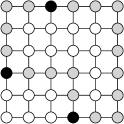
(b)

Figure 1.5: The 2D-GHZ game. The quantum circuit strategy (a) prepares $n^{2}$ qubits in the cluster state of the $n\times n$ grid. It takes inputs $x_{1},\dots,x_{n^{2}}\in\{1,2,3\}$, performs controlled Pauli measurements according to $1\mapsto X,2\mapsto Y,3\mapsto Z$, and returns outcomes $y_{1},\dots,y_{n^{2}}\in\{0,1\}$ according to $1\mapsto 0,-1\mapsto 1$. The input is randomly sampled as follows. First select nodes $A,B,C\in n\times n$ and paths $u_{AB},u_{BC},u_{CA}\subset n\times n$ in a “sufficiently uniform” way. The circuit wins if the output $y$ satisfies $x_{A}\oplus x_{B}\oplus x_{C}=1\oplus(y_{A}\oplus k_{A}(y))\oplus(y_{B}\oplus k_{B}(y))\oplus(y_{C}\oplus k_{C}(y))$, where $k_{A}(y),k_{B}(y),k_{C}(y)\in\{0,1\}$ depends only on the value of $y$ close to $A,B,C$ respectively.

Theorem [BGK18].

The shallow quantum circuit $\{Q_{n}\}_{n\in\mathbb{N}}$ solves the 2D-GHZ game perfectly for all $n$. However, the 2D-GHZ game is not solved with high accuracy by any classical shallow circuit $\{C_{n}\}_{n\in\mathbb{N}}$.

$$p_{S}(Q_{n},\text{2D-GHZ}(n)) =1$$ (1.6)

$$p_{S}(C_{n},\text{2D-GHZ}(n)) \leq 3/4+\epsilon_{n}$$ (1.7)

where $p_{S}$ denotes success probability and $\epsilon_{n}\in O(1/n)$.

The key to BGK’s result is that single-qubit measurements on an entangled state with only local entanglement can create entanglement between qubits that are far away. Depth and fan-in constrain the nonlocal correlations that a classical circuit can produce, but it also constrains the entangled states and the measurements that a quantum circuit can use. Observe that in the circuit $C_{\text{NC}}$ there can only be a path from input $x_{i}$ to output $y_{i}$, while in a circuit of depth $D$ and maximal fan-in $K$ there can be a path from at most $K^{D}$ inputs to any given output. As Verifier makes different choices of players $v_{A},v_{B},v_{C}$ in the 2D-GHZ game this forces the depth and fan-in of a classical circuit to be large. On the classical side it can be shown that when the measurement along the paths $u_{AB},u_{BC},u_{CA}$ are made, the effect is to create an entangled $\lvert GHZ\rangle$ state at qubits $v_{A},v_{B},v_{C}$, up to a local Pauli factors given by $k_{A},k_{B},k_{C}$. Furthermore, these corrections can be made classically post measurement.

In summary, the technique relies upon two key properties of the GHZ game: The use of the GHZ state and Pauli measurements. The choice of state is important because it can be realised by local measurements on a graph state in different ways, and the measurements are important because it allows for the corrections $k_{A},k_{B},k_{C}$ to be performed post-measurement.

Results

We first present a quantum protocol that uses teleportation to both distribute an entangled state on a graph and perform measurements on the distributed qudits (Figure 1.6). For any multi-qudit state $\psi$ with qudit $i$ and graph $G$ with nodes $V$ we consider a scenario where a number of agents $I\times V$, one for each qudit of $\psi$ and node of $G$, share entanglement. Each qudit of $\psi$ is held by some node on the graph, and each pair of nodes $(i,v),(i,w)$ such that $v,w$ are adjacent in $G$ share a two-qudit entangled state. By choosing a path through the graph for each qudit we can then distribute each qudit of $\psi$ to an arbitrary node on the graph, up to a random single-qudit phase for each qudit. An important observation is that this can be done in a constant number of rounds of quantum measurements.

(a)

(b)

Figure 1.6: Given a nonlocal game with players $I$ and state $\psi$, and a graph $G$ with nodes $V$ we consider the scenario (a) consisting of players $I\times V$, here each dotted circle indicate a player and $\bullet$ a qudit in either a maximally entangled state or the state $\psi$. (b) By performing local measurement on the qudits held by each player we can distribute each qudit, up to a random factor on each qudit, to any player on the graph.

We then consider the family of protocols arising from a fixed state and a family of graphs. Using this construction we show that any nonlocal game gives rise to a family of distributed games. We then show that for certain families of graphs distributed games gives rise to unconditional quantum advantage results with shallow circuits.

We present two versions of this construction. The first is completely general, but the distributed games have two rounds (Figure 1.9). It is a result about interactive circuits (Figure 1.3). The second result is less general, but for circuits in the usual sense having only a single round of inputs and outputs (Figure 1.8). In the second result we consider nonlocal games with quantum strategies given by measurements of single-qudit Weyl operators. Note that the states are still completely general.

The outline of the two results is as follows. Suppose that $(Q_{\text{NC}},\Phi)$ is any nonlocal game with classical bound $\gamma$. For any family of graphs $\{G_{n}\}_{n\in\mathbb{N}}$ we define a family of two-round cooperative games $\{\Phi_{n}\}_{n}$ and two-round interactive quantum circuits $\{Q_{n}\}_{n}$, such that for each $n\in\mathbb{N}$ the quantum circuit $Q_{n}$ violates the bound $\gamma$. For certain families of graphs we show that the quantum circuit is shallow and that a classical shallow circuit $\{C_{n}\}_{n}$ violates the bound $\gamma$ only up to a small factor $\epsilon_{n}$. Where $\text{lim}_{n\to\infty}\epsilon_{n}=0$. The rate of convergence is a property of the graphs.

Theorem I (Informal).

For any nonlocal game $\Phi$ and quantum strategy $Q$ we define a family of two-round interactive games $\{\Phi_{n}\}_{n\in\mathbb{N}}$ and a shallow two-round quantum circuit $\{Q_{n}\}_{n\in\mathbb{N}}$ such that for any classical two-round interactive shallow circuit $\{C_{n}\}_{n\in\mathbb{N}}$

$$p_{S}(Q_{n},\Phi_{n}) =p_{S}(Q,\Phi)$$ (1.8)

$$p_{S}(C_{n},\Phi_{n}) \leq\gamma+\epsilon_{n}$$ (1.9)

for some small $\epsilon_{n}$.

Next, we show that if the quantum strategy uses only single-qudit Weyl measurements (Figure 1.7)

Figure 1.7: A Weyl measurement strategy is a special quantum strategy using measurements in the basis of Weyl operators. For dimension $d\geq 2$ and $n$-qudit state $\psi$ the Weyl measurement strategy takes inputs $p_{1},\dots,p_{n}\in\mathbb{Z}_{d}^{2}$ and return outcomes $q_{1},\dots,q_{n}\in\mathbb{Z}_{d}$ of performing the single-qudit Weyl measurement $W(p_{i})$ on qudit $i$.

then the number of input-output rounds can be reduced to one.

Theorem II (Informal).

For any nonlocal game $\Phi$ and Weyl measurement strategy $Q$ we define a family of nonlocal games $\{\Phi_{n}\}_{n\in\mathbb{N}}$ and a shallow quantum circuit $\{Q_{n}\}_{n\in\mathbb{N}}$ such that for any classical shallow circuit $\{C_{n}\}_{n\in\mathbb{N}}$

$$p_{S}(Q_{n},\Phi_{n}) =p_{S}(Q,\Phi)$$ (1.10)

$$p_{S}(C_{n},\Phi_{n}) \leq\gamma+\epsilon_{n}$$ (1.11)

for some small $\epsilon_{n}$.

where $\epsilon_{n}$ is a different bound.

(a)

(b)

Figure 1.8: Let $\psi$ be an $I$-qudit state and $G=(V,E,r)$ a rooted graph. The quantum circuit strategy (a) prepares a single instance of $\psi$ and a maximally entangled pair of qudits $\lvert\phi\rangle:=\frac{\lvert 00\rangle+\lvert 11\rangle}{\sqrt{2}}$ for each $i\in I$ and edge $e\in E$. The circuit has an input for each $(i,v)\in I\times V$ which controls a measurement on a subset of qudits. This subset includes one of the two qudits of the state $\lvert\phi\rangle$ associated with each edge adjacent to $v$, and when $v=r$ also includes qudit $i$ of $\psi$. The possible measurement settings are either a Weyl operator measurement on a single qudit, or a Bell basis measurement on a pair of qudits. (b) In the nonlocal game Verifier selects inputs $p_{1},\dots,p_{n}$ and an accepting condition $A$ according to the nonlocal game $\Phi$. Verifier then randomly selects a rooted path $(v_{i1},\dots,v_{il_{i}})$ for each $i\in I$ and sends each $(i,v_{il_{i}})$ the input corresponding to a Bell basis measurement, and $(i,v_{il_{i}})$ the Weyl measurement setting $p_{i}$. Verifier accepts the outputs $p_{i1}^{\prime},\dots,p_{i(l_{i}-1)}^{\prime},q_{i}$ if $(q_{1}-[p_{1},p_{1}^{\prime}],\dots,q_{n}-[p_{n},p_{n}^{\prime}])\in A$, where $p_{i}^{\prime}:=p_{i1}^{\prime}+\dots+p_{il_{i}}^{\prime}$.

(a)

(b)

(c)

Figure 1.9: Let $\psi$ be an $I$-qudit state and $G=(V,E,r)$ a rooted graph. The quantum circuit strategy (a) prepares a single instance of $\psi$ and a maximally entangled pair of qudits $\lvert\phi\rangle:=\frac{\lvert 00\rangle+\lvert 11\rangle}{\sqrt{2}}$ for each $i\in I$ and edge $e\in E$. The circuit first takes an input for $(i,v)\in I\times V$ which controls a non-destructive measurement on a subset of qudits, it then takes another round of inputs for each $(i,v)\in I\times V$ which control destructive measurements on each subset of qudits. For each $(i,v)$ the subset of qudits which is measured includes one of the two maximally entangled qudits associated with each edge adjacent to $v$, and when $v=r$ also includes qudit $i$ of $\psi$. In the first round the measurement settings are either nothing or a Bell basis measurement on a pair of qudits. In the second round the possible measurements are either nothing or a conjugated measurement $W(p)MW(p)^{\dagger}$ on a single qudit, where $M$ is one of the measurement settings. (b) In the nonlocal game Verifier selects inputs $x_{1},\dots,x_{n}$ and an accepting condition $A$ according to the nonlocal game $\Phi$. Verifier then randomly selects a rooted path $(v_{i1},\dots,v_{il_{i}})$ for each $i\in I$ and first sends each $(i,v_{il_{i}})$ the input corresponding to a Bell basis measurement. If the outcomes of this are $p_{i1},\dots,p_{i(l_{i}-1)}$ Verifier sends $(i,v_{il_{i}})$ the input for the conjugated measurement $W(p_{i})M_{x_{i}}W(p_{i})^{\dagger}$, where $p_{i}^{\prime}:=p_{i1}^{\prime}+\dots+p_{il_{i}}^{\prime}$. Verifier accepts the output $y_{1},\dots,y_{n}$ if $(y_{1},\dots,y_{n})\in A$.

1.3 Structure of this text

In Chapter 2 we present some technical background material on the sheaf-theoretic framework. We then present the results on cohomology and circuits in Chapters 3 and 4 respectively, and we conclude with some remarks in Chapter 5.

Chapter 2 The sheaf-theoretic framework

An early influential paper on contextually is John Bell’s famous paper on the Einstein-Podolsky-Rosen (EPR) paradox [Bel64]. The “paradox” of EPR purportedly showed that quantum mechanics should not be seen as a complete description of physical reality [EPR35]. Bell’s insight could be understood to be that the incompleteness highlighted by EPR is not simply a feature of quantum mechanics, but of any physical theory that is consistent with the empirical predictions of quantum mechanics. Other influential papers by Kochen and Specker [KS75], Mermin [Mer90], and Greenberger-Horne-Zeillinger [GHSZ90], to mention a few.

This early work on contextuality focused on particular examples. Our interest in contextuality stems from the wish to prove general connections between contextuality and quantum advantage. It is therefore necessary to work with a more abstract definition of contextuality. Our approach uses the sheaf theoretic framework of Abramsky and Brandenberger [AB11]. The sheaf theoretic approach is among several general definitions of contextuality. For example, Robert Spekken’s ontological models framework [Spe05], Cabello, Severini, and Winter’s graph theoretic approach [CSW14], and the contextuality by default approach of Dzhafarov, Kujala, and Cervantes [DKC15]. Further work on the contextuality by default approach was carried out by Dzhafarov, Kujala, and Cervantes [DKC15] and connections with psychology were investigated by Dzhafarov and Kujala [DK16], to mention some. A graph theoretic approach that refines that of Cabelo, Severini and Winter’s is the approach of Acín, Fritz, Leverrier, and Sainz [AFLS15].

The sheaf theoretic framework has proved useful for linking contextuality to constraint satisfaction and database theory [AH12, Abr13].

In this chapter, we give an introduction to contextuality using the sheaf-theoretic framework, and we introduce several technical notions that will be used in the following chapters.

Overview

The two basic concepts in the sheaf theoretic framework are measurement scenarios and empirical models. We introduce measurement scenarios in Section 2.1 and empirical models in Section 2.2. In Section 2.3 we define simulations, a class of structure preserving transformations between empirical models. In Section 2.4.2 we introduce the Čech cohomology obstruction for contextuality. In Section 2.5 we define non-local games. In Section 2.6 we introduce the contextual fraction, and give an example of a resource inequality.

2.1 Measurement scenarios

Figure 2.1: Let $(X,\mathcal{M},O)$ be a measurement scenario. In an experimental run with $k$ rounds a sequence of contexts$\{x_{11},\dots,x_{1n_{1}}\},\dots,\{x_{k1},\dots,x_{kn_{k}}\}\in\mathcal{M}$ satisfying Eq. (2.1) are performed, giving outcomes $\{o_{11},\dots,o_{1n_{i}}\},\{o_{k1},\dots,o_{kn_{k}}\}$.

In the sheaf theoretic approach of Abramsky and Brandenberger [AB11] a measurement scenario represents the abstract type of an experiment. In this type of experiment some, but not necessarily all, combinations of measurements can be performed together, either sequentially or in parallel (Figure 2.1). We will first give the general definition and then consider two types of scenarios: quantum scenarios (Section 2.1.1) and multipartite scenarios (Section 2.1.2).

A measurement scenario is specified by a set of measurements, a family of subsets called the measurement cover specifying which measurements are compatible, and a set of outcomes for each measurement.

Definition 2.1.1.

A measurement scenario is a tuple $(X,\mathcal{M},\{O_{x}\}_{x\in X})$ where

• $X$ is a set of measurements.

• $\mathcal{M}\subset\mathcal{P}(X)$ is a family of subsets of measurements, called the measurement cover, such that:

  1. $\mathcal{M}$ covers $X$: $\bigcup_{C\in\mathcal{M}}C=X$.

  2. $\mathcal{M}$ is downwards closed: If $C\in\mathcal{M}$ and $C^{\prime}\subset C$ then $C^{\prime}\in\mathcal{M}$.

• $O_{x}$ is a set of outcomes.

The elements of the measurement cover are called contexts.

Let $(X,\mathcal{M},O)$ be a measurement scenario. Each context $C\in\mathcal{M}$ represents a set of compatible measurements that can be performed either sequentially in any order, or in parallel. We make the restriction that a measurement can only be performed once. A sequence of contexts $C_{1},\dots,C_{n}\in\mathcal{M}$ is valid if it has no repeated measurements and its union is a context:

$$\bigcup_{i}C_{i}\in\mathcal{M}\quad\text{ and }\quad C_{i}\cap C_{j}=\emptyset\quad\text{ for all }i\neq j$$ (2.1)

A joint outcome $s\in\prod_{x\in X^{\prime}}O_{x}$ to a subset of measurements is sometimes called a local section. This assignment is called the event sheaf.

Definition 2.1.2.

Let $S=(X,\mathcal{M},O)$ be a measurement scenario. The event sheaf, denoted by $\mathcal{E}_{S}$, assigns to each $U\subset X$ the set of local sections $\mathcal{E}(U):=\prod_{x\in U}O_{x}$, and for each $V\subset U$ restrictions $s\in\mathcal{E}(U)$ to a local section $s\rvert_{V}$ by the usual functional restriction.

Recall that a presheaf on a topological space $X$ is a contravariant function $F:X^{\text{op}}\to\text{Set}$. Here $X$ is seen as a category with objects given by the open sets, and morphisms inclusion. For each inclusion $U\subset V$ the map $F(U\subset V):F(V)\to F(U)$ is called the restriction map. A sheaf is a presheaf satisfying the following the sheaf condition. A compatible family for the open cover $\mathcal{U}$ is a family$\{f_{U}\in F(U)\}_{U\in\mathcal{U}}$ whose restrictions on overlaps are compatible:

$$F(U\cap V\subset U)(f_{U})=F(U\cap V\subset V)(f_{V})$$ (2.2)

for all $U,V\in\mathcal{U}$. The sheaf condition states that any compatible family arises as the family of restrictions

$$f_{U}=F(U\subset X)(f)$$ (2.3)

of some global section $f\in F(U)$.

2.1.1 Quantum scenarios

The first example of a measurement scenario that we work with arise from sets of projective measurements. A projective measurement is a family of projectors $M=\{M_{o}\}_{o\in O}$, where $O$ labels the outcomes, such that $\sum_{o\in O}M_{o}=I$. Two measurements $M=\{M_{o}\}_{o\in O}$, and $N=\{N_{p}\}_{p\in P}$ commute if their projective elements commute:

$$M_{o}N_{p}=N_{p}M_{o}\quad\text{for all $o\in O$, $p\in P$}$$ (2.4)

A set of pairwise commuting projective measurements is said to be compatible.

Example 2.1.1.

Let $\boldsymbol{M}$ be a set of projective measurements. $(\boldsymbol{M},\mathcal{M},O)$ is the measurement scenario with measurement cover the maximal subsets of pairwise commuting measurements, and outcomes $O$ given by the outcomes of each measurement.

The $n$-Pauli group, denoted by $P_{n}$, is the group of $n$-qubit unitary operators generated by the single-qubit Pauli operators

$$I:=\begin{bmatrix}1&0\\ 0&1\\ \end{bmatrix}\quad\sigma_{{x}}:=\begin{bmatrix}0&1\\ 1&0\\ \end{bmatrix}\quad\sigma_{{y}}:=\begin{bmatrix}0&-i\\ i&0\\ \end{bmatrix}\quad\sigma_{{z}}:=\begin{bmatrix}1&0\\ 0&-1\\ \end{bmatrix}$$

We denote the application of the Pauli operator $\sigma_{{p}}=\sigma_{{x}},\sigma_{{y}},\sigma_{{z}}$ to qubit $i$ as

$$\sigma_{{p}}^{i}=I\otimes\dots\otimes\sigma_{{p}}\otimes\dots\otimes I$$ (2.5)

recall that the single-qubit Pauli operators satisfy the commutativity relation

$$\sigma_{{x}}\sigma_{{y}}=-\sigma_{{y}}\sigma_{{x}}$$ (2.6)

$$\sigma_{{x}}\sigma_{{z}}=-\sigma_{{z}}\sigma_{{x}}$$ (2.7)

$$\sigma_{{y}}\sigma_{{z}}=-\sigma_{{z}}\sigma_{{y}}$$ (2.8)

It therefore follows that two $n$-qubit Pauli operators commute if and only if they anti-commute at an even number of qubits. An $n$-qubit Pauli operator specifies a projective measurement with outcomes $\{0,1\}$. Two $n$-qubit Pauli operators commute, and therefore their projective measurements there also commute, if and only if they anti-commute at an even number of qubits.

Example 2.1.2.

A quantum scenario $(\mathcal{O},\mathcal{M},\mathbb{Z})$ is given by the set of two-qubit Pauli operators

(2.15)

where each row and column make up a maximal context.

2.1.2 Multipartite scenarios

The second type of measurement scenario that we consider represents scenarios where measurements can be performed independently at a number of locations (Figure 2.2). This is sometimes called a non-locality scenario. We prefer the terminology “multipartite” because it avoids the implication that the locations are necessarily spatially separated.

A multipartite scenario is specified by a set of measurement sites $I$, for each measurement site $i$ a set of measurement settings $X_{i}$, and for each measurement setting $x\in X_{i}$ a set of measurement outcomes $Y_{i,x}$. Two measurements are compatible if and only if they belong to a different measurement site. First a comment about notation. Recall that $\coprod_{i\in I}X_{i}$ is defined as

$$\coprod_{i\in I}X_{i}:=\{(i,x)\mid i\in I,x\in X_{i}\}$$ (2.16)

Definition 2.1.3.

A multipartite scenario $(I,X,Y)$ is the measurement scenario $(\coprod_{i\in I}X_{i},\mathcal{M},Y)$, where the measurement cover $\mathcal{M}$ is defined by

$$\mathcal{M}:=\{C\subset\coprod_{i\in I}X_{i}\mid(i,x),(i,x^{\prime})\in C\Rightarrow x=x^{\prime}\}$$ (2.17)

and $Y_{i,x}$ is the set of outcomes for each $(i,x)$.

Figure 2.2: Consider a multipartite scenario with two measurement sites with measurement settings $\{a,a^{\prime}\}$, $\{b,b^{\prime}\}$ respectively. The maximal contexts are then $\{a,b\},\{a,b^{\prime}\},\{b^{\prime},a^{\prime}\},\{b,a^{\prime}\}$.

2.2 Empirical models

While a measurement scenario describes an experimental setup Abramsky and Brandenberger introduced the concept of an empirical model to capture the empirical data generated in an experiment. They introduced two types of empirical models, capturing different types of data. In Section 2.2.1 we define probabilistic empirical models, and probabilistic contextuality. In Section 2.2.2 we define possibilistic empirical models, and possibilistic contextuality.

2.2.1 Probabilistic empirical models

For any set $X$ write $\mathcal{D}(X)$ for the set of probability distributions over $X$. It is sometimes convenient to write a probability distribution $d\in\mathcal{D}(X)$ as a formal sum $d=\sum_{x\in X}d(x)\cdot x$ over the elements of $X$. Note that $\mathcal{D}$ is a functor with action on functions $f:X\to Y$ given by the pushforward

$$f_{*}:\mathcal{D}(X)\to\mathcal{D}(Y) ::\sum_{x\in X}d(x)\cdot x\mapsto\sum_{x\in X}d(x)\cdot f(x)$$ (2.18)

Let $S=(X,\mathcal{M},O)$ be a measurement scenario. Consider the assignment $U\mapsto\mathcal{D}(\mathcal{E}_{S}(U)$ of the set of probability distributions over the local sections at a set of measurements $U\subset X$. $\mathcal{D}\circ\mathcal{E}_{S}:X^{\text{op}}\to\text{Set}$ is a presheaf, but not in general a sheaf. For each $U\subset V$ and $d\in\mathcal{D}(\mathcal{E}_{S}(V)$ the restriction map is the marginal distribution $d\rvert_{U}\in\mathcal{D}(\mathcal{E}_{S}(U))$

$$d\rvert_{U}:=\sum_{s\in\mathcal{E}_{S}(V)}d_{s}\cdot s\rvert_{U}$$ (2.19)

where $s\rvert_{U}$ is the restriction of the section $s$ to $U$.

Definition 2.2.1.

Let $(X,\mathcal{M},O)$ be a measurement scenario. A probabilistic empirical model is a family of probability distributions $e=\{e_{C}\in\mathcal{D}(\mathcal{E}(C))\}_{C\in\mathcal{M}}$ such that

$$C\subset C^{\prime}\Rightarrow e_{C^{\prime}}\rvert_{C}=e_{C}$$ (2.20)

An experimental run for a scenario $S=(X,\mathcal{M},O)$ is a sequence $(C_{1},s_{1}),\dots,(C_{n},s_{n})$ where $C_{1},\dots,C_{n}\in\mathcal{M}$ is a valid sequence of contexts and $s_{1},\dots,s_{n}$ are local sections for the respective contexts. If $e$ is an empirical model then the probability of the run is

$$e(C_{1},s_{1},\dots,C_{n},s_{n}):=e(C_{1}\cup\dots\cup C_{n})(s_{1}\cup\dots\cup s_{n})$$ (2.21)

Local compatibility is motivated by the “no-disturbance” principle in quantum mechanics. For multipartite scenarios, this is more commonly called “no-signalling”. Let $\boldsymbol{M}$ be a set of projective measurements and $\psi$ a state. The measurement postulate of quantum mechanics defines an empirical model $e$ for the scenario $(\boldsymbol{M},\mathcal{M},O)$ given by

$$e(C)(s):=\lVert\big{[}\prod_{M\in C}M_{s(M)}\big{]}\psi\rVert^{2}$$ (2.22)

The no-disturbance principle is the observation that the probability distribution given by a context $C\subset\boldsymbol{M}$ is independent of which other compatible measurements it is performed in. Marginalising from the maximal contexts, therefore, gives the correct behavior for quantum measurements.

For a multipartite scenario, the measurement settings are not themselves quantum measurements. We, therefore, have to choose some interpretations of them as quantum measurements. To ensure that the measurements are compatible we do this on independent subsystems.

Definition 2.2.2.

Let $S=(I,X,Y)$ be a multipartite scenario. A quantum realised empirical model $e_{\psi,\pi}$ is given by an $I$-qudit state $\psi$, and a single-qudit measurement $\pi(i,x)$ for each $i\in I$, $x\in X_{i}$ with outcomes $Y_{i,x}$. $e_{\psi,\pi}$ is defined by

$$e(C)=\sum_{s\in\mathcal{E}_{S}(C)}\lVert\big{[}\bigotimes_{(i,x)\in C}\pi(i,x)_{s(i,x)}\big{]}\psi\rVert^{2}\cdot s$$ (2.23)

The following example of an abstract empirical model is taken from [AB11].

Example 2.2.1.

An empirical model for the two-partite scenario with measurement sites $A,B$ and measurement settings $\{a,a^{\prime}\},\{b,b^{\prime}\}$ respectively and outcome $\{0,1\}$ is given by the table

A B (0,0) (0,1) (1, 0) (1,1)

a b 1/2 0 0 1/2

a b’ 3/8 1/8 1/8 3/8

a’ b 3/8 1/8 1/8 3/8

a’ b’ 1/8 3/8 3/8 1/8

(2.24)

The entries of the table give a probability to the outcomes of each maximal context. If the measurement $a$ is performed on its own, then the probability of $0$ is $1/2$, which can be seen by marginalising from either context $(a,b)$ or $(a,b^{\prime})$.

$$P(a=0) =P((a,b)=(0,1),(0,0))=1/2+0$$ (2.25)

$$P(a=0) =P((a,b^{\prime})=(0,1),(0,0))=3/8+1/8=1/2$$ (2.26)

Contextuality

Although $\mathcal{D}\circ\mathcal{E}_{S}:X^{\text{op}}\to\text{Set}$ is a presheaf, it is not necessarily a sheaf. There can be compatible families that do not arise as a family of restrictions from a global section. Probabilistic contextuality is defined as the failure of an empirical model to be explained as a family of restrictions.

Definition 2.2.3.

Let $S=(X,\mathcal{M},O)$ be a measurement scenario and $e$ an empirical model. $e$ is contextual if there is no $d\in\mathcal{D}(\mathcal{E}_{S}(X))$ such that for all maximal contexts $C\in\mathcal{M}_{*}$

$$e_{C}=d\rvert_{C}$$ (2.27)

An example of contextuality can therefore be thought of as a family of locally compatible data that cannot be “glued together” to a consistent global picture of the data. We now give some examples.

Example 2.2.2.

Consider the multipartite scenario $(\{A,B\},\{0,1\},\{0,1\})$ with measurement sites $A,B$ and two measurement settings each with two outcomes. The empirical model given by the following probability table is contextual.

A B (0,0) (0,1) (1, 0) (1,1)

a b 1/2 0 0 1/2

a b’ 1/2 0 0 1/2

a’ b 1/2 0 0 1/2

a’ b’ 0 1/2 1/2 0

(2.28)

Proof.

Suppose that there exists a probability distribution $d$ over the global sections whose restriction to each maximal context gives the table. From the probability table we have that each of the following events occur with certainty:

$$d(a=b)=1$$ (2.29)

$$d(a=b^{\prime})=1$$ (2.30)

$$d(a^{\prime}=b)=1$$ (2.31)

$$d(a^{\prime}=b^{\prime})=0$$ (2.32)

However, this is not possible because the constraints are mutually exclusive. ∎

Example 2.2.1 (The GHZ model [GHSZ90]).

Consider the multipartite scenario $(\{0,1,2\},\{\mathbb{Z}_{2}\},\{\mathbb{Z}_{2}\})$ with three measurement sites, two measurement settings at each measurement site, and two outcomes for each measurement setting. Let $\lvert\text{GHZ}\rangle:=\frac{1}{\sqrt{2}}(\lvert 000\rangle+\lvert 111\rangle$ and $\pi$ the mapping of measurement setting $0$ to a Pauli $X$-basis measurement, and $1$ to a Pauli $Y$-basis measurement

$$\pi::=(i,0)\mapsto X,(i,1)\mapsto Y$$ (2.34)

The quantum realised empirical model $e_{\text{GHZ}}$ given by measurements $\pi$ on the state $\lvert GHZ\rangle$ is contextual.

Proof.

Write $X$ for the total set of measurements, suppose that there exists a probability distribution $d$ on the set of global sections $g:X\to\mathbb{Z}_{2}$ that gives the empirical model $e_{\text{GHZ}}$. $\lvert\text{GHZ}\rangle$ is a $+1$-eigenstate of $\sigma_{{x}}^{1}\sigma_{{x}}^{2}\sigma_{{x}}^{3}$ while it is a $-1$-eigenstate of $\sigma_{{x}}^{1}\sigma_{{y}}^{2}\sigma_{{y}}^{3}$, $\sigma_{{y}}^{1}\sigma_{{x}}^{2}\sigma_{{y}}^{3}$, and $\sigma_{{y}}^{1}\sigma_{{y}}^{2}\sigma_{{x}}^{3}$. With the identification $\{-1,1\}\cong\mathbb{Z}_{2}$ this means that any global section $g:X\to\mathbb{Z}_{2}$ satisfies

$$\sigma_{{x}}^{1}\oplus\sigma_{{x}}^{2}\oplus\sigma_{{x}}^{3} =0$$ (2.35)

$$\sigma_{{x}}^{1}\oplus\sigma_{{y}}^{2}\oplus\sigma_{{y}}^{3} =1$$ (2.36)

$$\sigma_{{y}}^{1}\oplus\sigma_{{x}}^{2}\oplus\sigma_{{y}}^{3} =1$$ (2.37)

$$\sigma_{{y}}^{1}\oplus\sigma_{{y}}^{2}\oplus\sigma_{{x}}^{3} =1$$ (2.38)

However, summing them together results in $0=1$. There is therefore no global section $g$, and in particular no distribution $d$. ∎

Another famous example is the so-called CHSH model [CHSH69]. This illustrates an important technique for proving contextuality. It uses an argument involving an inequality satisfied by all non-contextual models.

Example 2.2.3 (The CHSH model).

Consider the multipartite scenario $(\mathbb{Z}_{2},\{\mathbb{Z}_{2}\},\{\mathbb{Z}_{2}\})$ with two measurement sites, two measurement settings at each measurement site, and two outcomes for each measurement setting. The CHSH model, $e_{\text{CHSH}}$, is the empirical model realised by the state $\Phi:=\frac{1}{\sqrt{2}}(\lvert 00\rangle+\lvert 11\rangle)$ and

$$\pi::=\begin{cases}(0,0)\mapsto Z,\\ (0,1)\mapsto X,\\ (1,0)\mapsto A,\\ (1,1)\mapsto B\end{cases}$$ (2.39)

where

$$\lvert a_{0}\rangle :=\cos{\frac{\pi}{8}}\lvert 0\rangle+\sin{\frac{\pi}{8}}\lvert 1\rangle,\quad\lvert a_{1}\rangle:=-\sin{\frac{\pi}{8}}\lvert 0\rangle+\cos{\frac{\pi}{8}}\lvert 1\rangle$$ (2.40)

$$\lvert b_{0}\rangle :=\cos{\frac{\pi}{8}}\lvert 0\rangle-\sin{\frac{\pi}{8}}\lvert 1\rangle,\quad\lvert b_{1}\rangle:=\sin{\frac{\pi}{8}}\lvert 0\rangle+\cos{\frac{\pi}{8}}\lvert 1\rangle$$ (2.41)

Lemma 2.2.1.

The CHSH model is contextual. For any non-contextual model the sum $\sum_{x,y}x_{1}\oplus x_{2}=y_{1}\land y_{2}\leq 0.75$. For $e_{\text{CHSH}}$ the sum is $\cos^{2}{\frac{\pi}{8}}\approx 0.85>0.75$.

2.2.2 Possibilistic empirical models

(a) Hardy’s model

(b) PR-box

Figure 2.3: Bundle diagrams of Hardy’s model and the PR-box. The points above each measurement represents the two outcomes $0,1$ and the line segments the possible joint value assigmnets allowed by each model. A global section corresponds to a cycle visiting each measurement exactly once, for example the section $(a,a^{\prime},b,b^{\prime})=(1,1,0,0)$ in (a). However, (a) is logically contextual at the local section $(a,b)=(0,0)$ as can be seen. It can be seen that (b) is strongly contextual because no cycle visiting each measurement once is possible. .

Let $d\in\mathcal{D}(X)$ be a probability distribution over a set $X$. The support of $d$ is the subset ${\left\lvert d\right\rvert}:=\{x\in X\mid d(x)>0\}$.

Observe that examples 2.2.2 and 2.2.1 we do not refer to particular probabilities. The proofs show that there is no global section $s\in\mathcal{E}_{S}(X)$ that is consistent with the support of the models. Given any probabilistic empirical model $e$ we can “forget” about the probabilities and only consider the family of supports $\{{\left\lvert e_{C}\right\rvert}\subset\mathcal{E}_{S}(C)\}_{C\in\mathcal{M}_{*}}$. This is an example of a probabilistic empirical model. Probabilistic empirical models can be seen as presheafs in the following way.

Definition 2.2.4.

A possibilistic empirical model $\mathcal{S}:(X,\mathcal{M},O)$ is a subpresheaf of $\mathcal{E}_{S}$ such that

1. Every compatible family for the measurement cover $\mathcal{M}$ induces a global section.

2. $\mathcal{S}$ is flasque beneath the cover: If $C,C^{\prime}\in\mathcal{M}$ and $C\subset C^{\prime}$ then every $s\in\mathcal{S}(C)$ is the restriction of some $s^{\prime}\in\mathcal{S}(C^{\prime})$.

Note that although any probabilistic empirical model gives rise to a probabilistic empirical model, the converse is not necessarily true. Not all possibilistic empirical models is the support of a probabilistic model.

Possibilistic empirical models can be represented as boolean tables. An example is given by the Hardy model

A B (0,0) (0,1) (1, 0) (1,1)

a b 1 1 1 1

a b’ 0 1 1 1

a’ b 0 1 1 1

a’ b’ 1 1 1 0

(2.42)

and the Popescu-Rohrlich (PR) box.

A B (0,0) (0,1) (1, 0) (1,1)

a b 1 0 0 1

a b’ 1 0 0 1

a’ b 1 0 0 1

a’ b’ 0 1 1 0

(2.43)

In the possibilistic setting there are two natural forms of contextuality that we can consider. Logical and strong.

Definition 2.2.5.

Let $\mathcal{S}$ be a possibilistic empirical model for a measurement scenario $(X,\mathcal{M},O)$. We say that $\mathcal{S}$ is

• logically contextual at $s\in\mathcal{S}(C)$ if there is no global section $g\in\mathcal{S}(X)$ such that $g\rvert_{C}=s$.

• logically contextual if $\mathcal{S}$ is logically contextual at some local section. Otherwise, it is non-contextual.

• strongly contextual if $\mathcal{S}$ has no global section: $\mathcal{S}(X)=\emptyset$.

We consider three types of contextuality forming a hierarchy:

$$\text{Probabilistic Contextuality}<\text{Logical Contextuality}<\text{Strong Contextuality}$$ (2.44)

Possibilistic empirical models can be represented by bundle diagrams. When an empirical model is represented as a bundle diagram logical and strong contextuality have particularly elegant interpretations. Logical contextuality is the failure of a single line to extend to a path, and strong contextuality is the property of every line extending to a path (Figure 2.3).

Lemma 2.2.2.

The Hardy model (2.42) is logically contextual, but not strongly contextual. The PR-box is strongly contextual.

Proof.

This can be seen by inspecting the bundle diagrams. ∎

2.2.3 State dependent contextuality

Let $\boldsymbol{M}$ be a set of projective measurements, $C\subset\boldsymbol{M}$ a context of commuting measurements, and $\psi$ a state. An outcome assignment $s$ for $C$ is consistent with $\psi$ if $s$ has non-zero probability according to the measurement postulate

$$\big{[}\prod_{M\in\boldsymbol{M}}M_{s(M)}\big{]}\psi\neq 0$$ (2.45)

Definition 2.2.6.

Let $\boldsymbol{M}$ be a set of projective measurements and $\psi$ a state. The state dependent model $\mathcal{S}_{\boldsymbol{M},\psi}$ is the possibilistic empirical model

$$\mathcal{S}_{\boldsymbol{M},\psi}(V):=\{s\in\mathcal{E}_{\boldsymbol{M},\mathcal{M},O}(V)\mid\text{$s$ is consistent with $\psi$}\}$$ (2.46)

The set of measurements $\boldsymbol{M}$ is state dependently contextual if $\mathcal{S}_{\boldsymbol{M},\psi}$ is contextual for some state $\psi$. An example of a state-dependent contextuality proof is the GHZ-example.

2.2.4 State independent contextuality

For some sets of quantum measurements, the state $\psi$ is not needed for the proof of contextuality.

Definition 2.2.7.

Let $\boldsymbol{M}$ be a set of projective measurements. The state independent model $\mathcal{S}_{X}$ is defined at any below the cover by

$$\mathcal{S}_{X}(V):=\{s\in\mathcal{E}_{\boldsymbol{M},\mathcal{M},O}(V)\mid\text{$s$ is consistent with \emph{some} state}\}$$ (2.47)

The set of measurements $\boldsymbol{M}$ is said to be state-independently contextual if $\mathcal{S}_{X}$ is contextual.

Example 2.2.2 (Mermin’s square [Mer90]).

Let $\mathcal{S}_{X}:(X,\mathcal{M},\mathbb{Z}_{2})$ be the state independent model induced by the set of measurements displayed in Mermin’s square

$\sigma_{{x}}^{1}$	$\sigma_{{x}}^{2}$	$\sigma_{{x}}^{1}\sigma_{{x}}^{2}$	$I$
$\sigma_{{z}}^{2}$	$\sigma_{{z}}^{1}$	$\sigma_{{z}}^{1}\sigma_{{z}}^{2}$	$I$
$\sigma_{{x}}^{1}\sigma_{{z}}^{2}$	$\sigma_{{z}}^{1}\sigma_{{x}}^{2}$	$\sigma_{{y}}^{1}\sigma_{{y}}^{2}$	$I$
$I$	$I$	$-I$

Observe that the measurements displayed in any row or column $M_{1},M_{2},M_{3},M_{4}$ defines a context and furthermore satisfies $M_{1}M_{2}M_{3}=M_{4}$, where $M_{4}=\pm I$. By Lemma 2.1 any local section $s\in\mathcal{S}(C)$ therefore satisfies one of the following equations

$$\sigma_{{x}}^{1}\oplus\sigma_{{x}}^{2}\oplus\sigma_{{x}}^{1}\sigma_{{x}}^{2} =0$$ (2.48)

$$\sigma_{{z}}^{1}\oplus\sigma_{{z}}^{2}\oplus\sigma_{{z}}^{1}\sigma_{{z}}^{2} =0$$ (2.49)

$$\sigma_{{x}}^{1}\oplus\sigma_{{z}}^{2}\oplus\sigma_{{x}}^{1}\sigma_{{z}}^{2} =0$$ (2.50)

$$\sigma_{{z}}^{1}\oplus\sigma_{{x}}^{2}\oplus\sigma_{{z}}^{1}\sigma_{{x}}^{2} =0$$ (2.51)

$$\sigma_{{x}}^{1}\sigma_{{z}}^{2}\oplus\sigma_{{z}}^{1}\sigma_{{x}}^{2}\oplus\sigma_{{y}}^{1}\sigma_{{y}}^{2} =0$$ (2.52)

$$\sigma_{{x}}^{1}\sigma_{{x}}^{2}\oplus\sigma_{{z}}^{1}\sigma_{{z}}^{2}\oplus\sigma_{{y}}^{1}\sigma_{{y}}^{2} =1$$ (2.53)

Any global section $g\in\mathcal{S}_{X}(C)$ therefore simultaneously satisfies all equations. However, these equations are mutually inconsistent. Summing together all of the equations gives $0=1$, because each measurement appears in exactly two equations. $\mathcal{S}_{X}$ is therefore strongly contextual.

2.3 Simulations

Figure 2.4: Consider a setup involving two measurement scenarios $S=(X,\mathcal{M},O),T=(Y,\mathcal{N},P)$. A simulation from $S$ to $T$ maps each measurement $y\in Y$ to a measurement protocol on $S$, and each possible outcome of this protocol to an outcome $p\in P_{y}$. This induces a map on empirical models of $S$ to empirical models of $T$.

The motivation behind introducing simulations is to equip the sheaf-theoretic framework with a class of structure-preserving transformations. The problem of what the right notion of structure-preserving transformation is for empirical models was considered by Karvonen [Kar19]. The work of Karvonen later formed the basis for the more developed idea of simulation laid out by Abramsky, Barbosa, Karvonen, and Mansfield [ABKM19a]. See also For further work on simulations see the work of Barbosa, Karvonen, and Mansfield [BKM21] and Abramsky, Barbosa, Karvonen, and Mansfield [ABKM19b].

The notion of simulation that we present here was defined by Abramsky et al. [ABKM19a], based on earlier work by The idea of studying examples of contextuality up to a class of structure-preserving transformations have also been considered by others, for example Amaral et al.  [ACCA18].

Informally, a simulation $s$ from a measurement scenario $S$ to another scenario $T$ describes how we can translate measurements on $T$ into measurements on $S$, and outcomes of these measurements on $S$ into outcomes in $T$ (Figure 2.4). This defines a map at the level of empirical models called the pushforward.

This section is structured as follows. In Section 2.3.1 we introduce the most simple example of a simulation, deterministic single-round simulations. We then introduce measurement protocols, describing adaptive sequence of measurements. We finally present the general notion of simulation.

2.3.1 Single-round simulations

We will now present the notion of simulation that Karvonen [Kar19] considered.

Definition 2.3.1.

A deterministic single-round simulation from a measurement scenario $S=(X_{S},\mathcal{M}_{S},O_{S})$ to another measurement scenario $T=(X_{T},\mathcal{M}_{T},O_{T})$ is a pair

$$f :X_{T}\to\mathcal{M}_{S}$$ (2.54)

$$g =\{g_{y}:\mathcal{E}_{S}(f(x))\to(O_{T})_{x}\}_{x\in X_{T}}$$ (2.55)

such that $\bigcup_{x\in C}f(x)\in\mathcal{M}_{S}$ for every $C\in\mathcal{M}_{T}$.

Let $e$ be an empirical model for the scenario $S$. The pushforward $(f,g)_{*}(e)$ is then the empirical model for the scenario $T$, defined by

$$(f,g)_{*}(e)(C):=\sum_{s\in\mathcal{E}_{S}(\cup_{x\in C}f(x))}e(\cup_{x\in C}f(x))(s)\cdot(x\mapsto g_{x}(s\rvert_{f(x)})$$ (2.56)

for all contexts $C$ in $T$. Suppose now that $e$ is non-contextual, and therefore a convex combination of global sections

$$e(C)=\sum_{\lambda\in\mathcal{E}(X_{S})}p_{x}\cdot\lambda\rvert_{C}$$ (2.57)

$(f,g)_{*}(e)$ is then a convex combination

$$(f,g)_{*}(e)(C)=\sum_{\lambda\in\mathcal{E}(X_{S})}p_{\lambda}\cdot g_{U}(\lambda\rvert_{f(U)})$$ (2.58)

If we define the global section $\lambda^{\prime}\in\mathcal{E}_{T}(Y)$ by

$$\lambda^{\prime}(y)=g_{y}(\lambda\rvert_{C_{y}})$$ (2.59)

for each global section $\lambda\in\mathcal{E}(X_{S})$, then

$$g_{U}(\lambda\rvert_{f(U)})=\lambda^{\prime}\rvert_{U}$$ (2.60)

hence $e$ is a convex combination of global sections, and hence non-contextual.

We, therefore, observe that if translate each measurement $y\in Y$ into a fixed measurement $f(y)\subset\mathcal{M}$ that is independent of the measurement context that $y$ is performed in, then the induced map on empirical models preserve non-contextuality. A simulation extends this in two ways, by allowing for randomness and several rounds of measurements.

2.3.2 Measurement protocols

While Karvonen initially only considered single-round simulations it is natural to consider simulations with more than one round of measurements. To capture this Abramsky, Mansfield, Barbosa, and Karvonen introduced what they called measurement protocols.

A measurement protocol of length $n$ on a measurement scenario $S$

$$C=\{C_{1},\dots,C_{i}(s_{1},\dots,s_{i-1}),\dots,C_{n}(s_{1},\dots,s_{n-1})\in\mathcal{M}_{X}\}_{s_{1}\in C_{1},\dots,(s_{1},\dots,s_{n-1})\in C_{n-2}(s_{1},\dots,s_{n-2})}$$ (2.61)

represents a deterministic strategy that someone can follow to perform measurements on $S$, in an adaptive way. The measurement setting $C_{i}$ is a function of the previous $i-1$ measurement outcomes. We require that for all outcomes $s_{1},\dots,s_{n-1}$ the sequence of contexts is valid, that is satisfying Eq. 2.1. We write $\text{MP}_{n}(S)$ for the set of measurement protocols of length $n$. A run of an adaptive measurement sequence $\{C_{i}(s_{1},\dots,s_{i-1})\}_{n\in\mathbb{N}}$ is a sequence of contexts and local sections $\{(U_{i},s_{i})\}_{n\in\mathbb{N}}$ such that $s_{i}\in\mathcal{E}_{S}(U_{i})$ and $U_{i}=C_{i}(s_{1},\dots,s_{i-1})$ for all $i\in\mathbb{N}$. We write $\mathcal{E}_{S}(C)$ for the set of runs of a measurement protocol $C$.

A set of measurement protocols $\{C^{j}\}_{j\in J}$ that can be performed in parallel is said to be compatible. For any compatible set of measurement protocols $\{C^{j}\}_{j\in J}$ their parallel product is denoted by $\otimes_{i\in I}C^{j}$.

When a measurement protocol $C$ is performed the outcome is a run. By the no-disturbance assumption the probability of a given run can be defined by

$$e(C)(r):=e(U_{1}\cup\dots\cup U_{n})(s_{1}\cup\dots\cup s_{n})$$ (2.62)

where $r=\{(U_{i},s_{i})\}_{i=1}^{N}$ is a run.

2.3.3 General simulations

The idea of describing probabilistic simulations as probability distributions over deterministic simulations is how Karvonen described simulations. Although only for single-round simulations. Later this was also how Abramsky, Barbosa, Mansfield, and Karvonen formalised probabilistic simulations with more than one round.

We now define deterministic $n$-round simulations, and general simulations as probability distributions over deterministic simulations.

Definition 2.3.2.

A deterministic simulation from a measurement scenario $S$ to another measurement scenario $T$ of depth $n$ is a pair $(f,g)$ where

• $f:X_{T}\to\text{MP}_{n}(S)$ is a function such that $\{f(x)\}_{x\in C}$ is compatible for all $C\in\mathcal{M}_{T}$.

• $g=\{g_{x}:\mathcal{E}(f(x))\to(O_{T})_{x}\}_{x\in X_{T}}$ is a family of functions.

Let $S=(X,\mathcal{M},O)$, $T=(Y,\mathcal{N},P)$ be two measurement scenarios, and $t=(f,g):S\to T$ a deterministic $n$-round simulation. For each context $C\in\mathcal{N}$ write $f_{C}$ for the parallel product of the measurement protocols $\{f(y)\}_{y\in C}$

$$f_{C}:=\otimes_{y\in C}f(y)$$ (2.63)

The family of functions $\{g_{y}\}_{y\in C}$ defines a function

$$g_{C}:\mathcal{E}_{S}(f_{C})\to\mathcal{E}_{T}(C)$$ (2.64)

defined at each $y\in C$ by the function $g_{y}$. For any empirical model $e$ of $S$ we define the pushforward $t_{*}(e)$ to be the empirical model for the scenario $T$ given by the convex combination

$$t_{*}(e)_{C}:=\sum_{r\in\mathcal{E}_{S}(f(C))}e(f(C))(r)\cdot g_{C}(r)$$ (2.65)

for each context $C$ of $T$.

Definition 2.3.3.

Let $S$ and $T$ be measurement scenarios. An $n$-round simulation from $S$ to $T$, denoted $s:S\to T$, is a probability distribution over the set of deterministic $n$-round simulations from $S$ to $T$.

We generalise the definition of the pushforward model by taking the convex combination of empirical models:

$$s_{*}(e)=\sum_{t:S\to T}s(t)\cdot t_{*}(e)$$ (2.66)

where $s=\sum_{t:S\to T}s(t)\cdot t$ is a simulation, and $e$ is an empirical model.

2.4 The cohomology of contextuality

A cohomology theory assigns an algebraic invariant to each element of some class of objects. Cohomology theories are useful when one can find invariants that can be computed easily, yet characterise an important property of the objects we are studying. An example is the simplicial cohomology of a topological space. Using for example triangulation we can compute the simplicial cohomology of a large class of spaces. In topology this is an invaluable tool for resolving many questions in a simple way.

In the sheaf-theoretic framework, a possibilistic empirical model is a sheaf of sets $\mathcal{S}:X^{\text{op}}\to\textbf{Set}$. Contextuality is seen as the failure of a local section $s\in\mathcal{S}(C)$ to extend to a global section $g\in\mathcal{S}(X)$. For presheafs of abelian groups $\mathcal{F}:X^{\text{op}}\to\textbf{AbGrp}$ this transition from local to global is characterised by a cohomological obstruction. It is therefore natural to consider if this obstruction can detect contextuality. Abramsky et al. showed that this is the case in a range of examples [AMB12], but also that it is not complete. A more precise characterisation of the class of models where it is complete was later given [ABK⁺15].

In this section we present the Čech cohomology obstruciton of Abramsky et al. [AMB12]. We first define the cohomology groups of a cochain complex in Section 2.4.1. In Section 2.4.2 we define the Čech cohomology groups of a presheaf of abelian groups. In Section 2.4 we define the obstruction for contextuality.

2.4.1 Cohomology groups of a cochain complex

To define the cohomology groups of an object we use a family of abelian groups connected by homomorphisms. This is called a cochain complex.

Definition 2.4.1.

A cochain complex is a sequence

(2.67)

where $C^{0},C^{1},\dots$ are abelian groups, and $d^{0},d^{1},\dots$ are homomorphisms such that $d^{n+1}\circ d^{n}=0$. The elements of $C^{n}$ are known as the $n$-cochains and $d^{n}$ is the $n$’th coboundary map. $\text{im}(d^{n})$ are the $n$-coboundaries and $\text{ker}(d^{n+1})$ the $n$-cocycles.

The requirement that $d^{n+1}\circ d^{n}=0$ equivalently says that every $n$-coboundary is an $n$-cocycle, $\text{im}(d^{n})\subset\text{ker}(d^{n+1})$. A sequence such that $\text{im}(d^{n})=\text{ker}(d^{n+1})$ is said to be exact at $n$. Cohomology measures the failure of a sequence to be exact.

Definition 2.4.2.

The $n$-th cohomology group is the quotient of the coboundaries to the cocycles. $H^{n}:=\text{im}(d^{n})/\text{ker}(d^{n-1})$.

The cohomology class $[x]\in H^{n}$ of a cocycle $x$ can be thought of as an obstruction for $x$ to be a coboundary, because $[x]=0$ if and only if $x$ is a coboundary.

When we assign a cochain complex to some mathematical object it is common to use a free construction. This free construction loses some of the structure of the original object. However, it can also be the case that the cohomology groups capture some interesting feature of the object. The classic example is simplicial cohomology, which relates to the number of “holes” in a topological space.

2.4.2 Čech cohomology

Let $X$ be a topological space, and $\mathcal{F}:X^{\text{op}}\to\mathbf{AbGrp}$ a presheaf of abelian groups. In this section we define the Čech cohomology groups of $\mathcal{F}$. To do this we assign to $\mathcal{F}$ a cochain complex. This complex is defined using an open cover $\mathcal{U}$ of $X$. First, we define an object encoding the combinatorial structure of the open cover.

Definition 2.4.3.

Let $\mathcal{U}$ be an open cover of a topological space $X$. The $n$-simplices of the nerve of $\mathcal{U}$, denoted by $\mathcal{N}_{n}(\mathcal{U})$, are $n+1$-tuples of intersecting open sets.

$$\mathcal{N}_{n}(\mathcal{U}) :=\{(U_{0},\dots,U_{n})\in\mathcal{U}^{n+1}\mid U_{0}\cap\dots\cap U_{n}\neq\emptyset\}$$ (2.68)

The boundary maps $\partial_{i}:\mathcal{N}_{n+1}(\mathcal{U})\to\mathcal{N}_{n}(\mathcal{U})$ remove the $i$’th open set:

$$\partial_{i}::(U_{0},\dots,U_{n+1})\mapsto(U_{0},\dots,U_{i-1},U_{i+1},\dots,U_{n+1})$$ (2.69)

Let ${\left\lvert(U_{0},\dots,U_{n})\right\rvert}:=\cap_{i}U_{i}$.

Definition 2.4.4.

Let $X$ be a topological space, $\mathcal{U}$ an open cover of $X$ and $\mathcal{F}$ a presheaf of abelian groups on $X$. The Čech cohomology group $H^{n}(\mathcal{F})$ is the $n$’th cohomology group of the cochain complex

(2.70)

where

• The $n$-cochains $C^{n}(\mathcal{U},\mathcal{F}):=\bigoplus_{U\in\mathcal{N}_{n}(\mathcal{U})}\mathcal{F}({\left\lvert U\right\rvert})$.

• The coboundary map $d^{n}(\omega)(U):=\sum_{i=0}^{q}{(-1)}^{i}\mathcal{F}({\left\lvert\partial_{i}U\right\rvert}\subset U)(\omega(\partial_{i}U))$

It can be verified that $d^{q+1}\circ d^{q}=0$.

2.4.3 The obstruction to the extension of a local section

Let $S=(X,\mathcal{M},O)$ be a measurement scenario, $\mathcal{S}$ a possibilistic empirical model, and $s_{0}\in\mathcal{S}(C_{0})$ a local section. We define the Čech cohomology obstruction for $s_{0}$ to extend to a global section.

We can give $\mathcal{S}$ the structure of an abelian presheaf by composing with the the functor $F_{\mathbb{Z}}:\textbf{Set}\to\textbf{AbGrp}$ assigning to each set $X$ the free abelian group on $X$, that is, the group of formal linear combinations of $X$.

$$F_{\mathbb{Z}}(X) :=\{\sum_{x\in X}k_{x}\cdot x\mid k_{x}\neq 0\text{ for finitely many $x\in X$}\}$$ (2.71)

$$F_{\mathbb{Z}}(f:X\to Y) :=\sum_{x\in X}k_{x}\mapsto\sum_{x\in X}k_{x}\cdot f(x)$$ (2.72)

Let $\mathcal{F}:=F_{\mathbb{Z}}\circ\mathcal{S}$. Note that even though $\mathcal{S}$ is a sheaf, $\mathcal{F}$ is generally only a presheaf.

The construction employs two auxiliary presheaves. For any subset $U\subset X$ we define $\mathcal{F}\rvert_{C_{0}}$ to be the restriction of each $U$ to $U\cap C_{0}$, and $\mathcal{F}_{\tilde{C_{0}}}$ assigns to each $U$ the subset of elements whose restriction to $U\cap C_{0}$ vanishes.

Definition 2.4.5.

Let $\mathcal{F}$ be an abelian presheaf and $C_{0}$ an open set.

$$\mathcal{F}_{\tilde{C_{0}}}::U\mapsto\ker{\mathcal{F}(U\cap C_{0}\subset U)}\quad\mathcal{F}\rvert_{C_{0}}::U\mapsto\mathcal{F}(C_{0}\cap U)$$ (2.73)

At any $U\subset X$ these presheaves are related to $\mathcal{F}$ by a sequence

which in fact is exact, because $\mathcal{F}$ is flasque beneath the cover. When lifted to the level of cochain complexes it, therefore, gives rise to a short exact sequence

Using standard techniques from homological algebra this short exact sequence of cochain complexes induces a long exact sequence of cohomology groups

where $\gamma$ is the connecting homomorphism. For details about this see for example [Wei94]. Using the identification $\mathcal{F}(C_{0})\cong H^{0}(\mathcal{M},\mathcal{F}\rvert_{C_{0}})$ we define the obstruction for $s_{0}$ to extend to a global section to be $\gamma(1\cdot s_{0})\in H^{1}(\mathcal{M},\mathcal{F}_{\tilde{C_{0}}})$.

Lemma 2.4.1 ([AMB12]).

If the cover $\mathcal{M}$ is connected then $\gamma(1\cdot s_{0})=0$ if and only if $1\cdot s_{0}$ extends to a compatible family of $F_{\mathbb{Z}}\mathcal{S}$.

Definition 2.4.6.

Let $\mathcal{S}:(X,\mathcal{M},O)$ be a possibilistic empirical model and $s_{0}\in\mathcal{S}(C_{0})$ a local section. The cohomological obstruction to $s_{0}$ lifting to a global section is the cohomological obstruction to $1\cdot s_{0}$ extending to a compatible family in $F_{\mathbb{Z}}\circ\mathcal{S}$.

Observe that if $s_{0}$ extends to a global section $s$ in $\mathcal{S}$, then $1\cdot s_{0}$ extends to a global section $1\cdot s$ in $\mathcal{F}$, hence the obstruction is sound.

Lemma 2.4.2.

The Čech cohomology obstruction for contextuality is sound: If $\gamma(g)\neq 0$ then $\mathcal{S}$ is logically contextual at $s$.

2.4.4 Generalised AvN arguments

The Čech cohomology obstruction is not complete. There are so-called false negatives, contextual empirical models where the obstruction vanishes. The approach detects contextuality in many cases, but an example where the approach is not complete is Hardy’s paradox. Work has been carried out by Caru on understanding false negatives and refining the approach [Car18].

The Čech cohomology obstruction is complete for a large fragment of models that can be described by generalised AvN models. Abramsky et al. [ABK⁺15] take this terminology from Mermin [Mer90] who used the term “all versus nothing” to describe his proof of contextuality. These proofs can be understood as exhibiting an inconsistent set of equations over $\mathbb{Z}_{2}$ that is locally satisfied by the model. The all versus nothing terminology was also used by for example Cabello [Cab01]. The Čech cohomology obstruction is complete for the generalised AvN models, the class of models that locally satisfies a system of inconsistent equations over any ring $R$ [ABK⁺15].

Definition 2.4.7.

Let $(X,\mathcal{M},R)$ be a measurement scenario where $R$ is a ring. An $R$-linear equation is a triple $(C,r,a)$ where $C\in\mathcal{M}$ is a context, $r:C\to R$ assigns a coefficient in $R$ to each $x\in C$, and $a\in R$ is a constant. A local section $s:C\to R$ satisfies $(C,r,a)$ if

$$\sum_{x\in C}r(x)\cdot s(x)=a$$ (2.74)

where $\cdot$ denotes multiplication in $R$.

Let $\mathcal{S}$ be an empirical model. The $R$-linear theory of $\mathcal{S}$ is the set of all $R$-linear equations that are consistent with $\mathcal{S}$.

$$\text{Th}_{R}(\mathcal{S}):=\bigcup_{C\in\mathcal{M}}\{(C,r,a)\mid s\text{ satisfies $(C,r,a)$ for all $s\in\mathcal{S}(C)$}\}$$ (2.75)

Definition 2.4.8.

$\mathcal{S}$ is $\text{AvN}_{R}$ if its $R$-linear theory is inconsistent. i.e. there is no $s:X\to R$ such that $s\rvert_{C}\models\phi$, for every context $C\in\mathcal{M}$ and formula $\phi\in\text{Th}_{R}(\mathcal{S})$ at $C$.

Theorem 2.4.1 ([ABK⁺15]).

If $\mathcal{S}$ is $\text{AvN}_{R}$ then $\gamma(1\cdot s)\neq 0$ for all $C\in\mathcal{M}$ and $s\in\mathcal{S}(C)$.

2.5 Witnessing contextuality through cooperative games

(a)

	$a=1$	$a=2$	$a=3$
$b=1$	$X_{1}$	$X_{2}$	$X_{1}X_{2}$
$b=2$	$Z_{2}$	$Z_{1}$	$Z_{1}Z_{2}$
$b=3$	$-X_{1}Z_{2}$	$-Z_{1}X_{2}$	$Y_{1}Y_{2}$

(b)

Figure 2.5: The Magic Square game. Alice and Bob each hold one of the two qubits of two maximally entangled states $\phi$. Verifier sends Alice and Bob $a,b\in\{1,2,3\}$. Alice performs the three observables $(M_{1},M_{2},M_{3})$ in column $b$ of (b) and Bob performs the observables in row $a$. Given outcome $x=(x_{1},x_{2},x_{3}),y=(y_{1},y_{2},y_{3})$ they win if $x_{1}\oplus x_{2}\oplus x_{3}=1$ and $y_{1}\oplus y_{2}\oplus y_{3}=0$, and $x_{b}=y_{a}$.

There are different ways of proving that an empirical model is contextual. For example, using inequalities [CHSH69, Bel64] or using systems of logical formulas [Mer90]. A systematic treatment of contextuality proofs is given by Abramsky and Hardy [AH12]. It is well known that certain contextuality proofs can be recast as cooperative games known as non-local games. For example, the Magic Square game (Figure 2.5) [CHTW10].

In this section, we first define cooperative games and non-local games. We then explain that simulations can be used to translate a cooperative game from one scenario to another.

2.5.1 Cooperative games

Let $S=(I,X,Y)$ be a multipartite scenario.

A game is played by $I$, thought of as players, against Verifier. A game is played over one or more rounds of the following form. Verifier sends each player $i\in I^{\prime}$, in a subset $I^{\prime}\subset$, a value $x_{i}\in X_{i}$, and each player responds with a value $y_{i}\in Y_{x}$. We assume that the players are not allowed to communicate and that each player is sent at most one value. A strategy for Verifier is therefore an $n$-round measurement protocol $C$, and a strategy for the players is an empirical model $e$.

At the beginning of each game Verifier randomly selects a strategy $C$ and an accepting condition $A\subset\mathcal{E}_{S}(m)$. The goal of the players is to maximize the probability that their responses $s_{1},\dots,s_{n}$ satisfies the accepting condition.

Definition 2.5.1.

Let $S=(I,X,Y)$ be a multipartite measurement scenario. An $n$-round game is a convex combination $\Phi=\sum_{C\in\text{MP}_{n}(S),A\subset\mathcal{E}_{S}(C)}\Phi_{C,A}\cdot(m,A)$. The success probability of an empirical model $e$ is

$$p_{S}(e,\Phi):=\sum_{C\in\text{MP}_{n}(S),A\subset\mathcal{E}_{S}(C)}\Phi_{C,A}e(C)(A)$$ (2.76)

A non-local game is a single-round cooperative game along with a quantum strategy exceeding that of any non-contextual strategy.

Definition 2.5.2.

Let $S=(I,X,Y)$ be a multipartite scenario. A non-local game is a pair $(e,\Phi)$ where $e$ is a quantum realised empirical model, and $\Phi$ is a single-round game, such that there exists a $\gamma$ such that for all non-contextual empirical models $e_{\text{NC}}$

$$p_{S}(e_{\text{NC}},\Phi)\leq\gamma<p_{S}(e,\Phi)$$ (2.77)

the least such $\gamma^{*}$, is called the classical upper bound.

A well-known example is the Greenberger-Horne-Zeillinger (GHZ) game [GHSZ90].

Example 2.5.1.

The GHZ game is played by three players $A,B,C$. Verifier selects inputs $x_{A},x_{B},x_{C}\in\mathbb{Z}_{2}$ with uniform probability. The players win if their outputs $y_{A},y_{B},y_{C}\in\mathbb{Z}_{2}$ satisfies

$$A_{\text{GHZ}}(x_{A},x_{B},x_{C})(y_{A},y_{B},y_{C})\iff x_{A}\lor x_{B}\lor x_{B}=y_{A}\oplus y_{B}\oplus y_{C}$$ (2.78)

A winning quantum strategy is given where each player performs a Pauli $X$ measurement if the input is $0$ and a Pauli $Y$ measurement if the input is $1$. However, any non-contextual strategy solves the game with at most $3/4$.

2.5.2 The pullback of a game

Figure 2.6: The pullback of a game $\Phi$. Consider a game where Verifier plays against a set of players $Y$. Verifier sends $Y$ a context $C$, the players then interact with another set of players $X$ through a measurement protocol $f(C)$. If the result of $f(C)$ is a run $r$ then they respond with $g_{C}(r)$ to Verifier. Verifier accepts if $g_{C}(r)\in A$ satisfies the accepting condition. This game is equivalent to the game where Verifier interacts directly with $X$ by performing the measurement protocol $f(C)$ and accepts a run $r$ if $r\in g_{C}^{-1}(A)$.

Let $S$ and $T$ be measurement scenarios, and $s:S\to T$ an $n$-round simulation. We have explained that $s$ induces a map on empirical models going from $S$ to $T$, called the pushforward. Simulations also have a natural action on games (Figure 2.6). The pullback $s^{*}$ maps $k$-round games of $T$ to $kn$-round games on $S$.

The defining property of the pullback is that for any empirical model $e$ of $S$ and game $\Phi$ of $T$, the success probability of $e$ on $s^{*}(\Phi)$ is the success probability of $s_{*}(e)$ on $\Phi$:

$$p_{S}(e,s^{*}(\Phi))=p_{S}(s_{*}(e),\Phi)$$ (2.79)

We can define the pullback directly as follows.

Definition 2.5.3.

Let $S$ and $T=(Y,\mathcal{N},P)$ be measurement scenarios, $s:S\to T$ an $n$-round simulation, and $\Phi$ a single-round game. The pullback $s^{*}(\Phi)$ is the $n$-round game for the scenario $S$, defined as

$$s^{*}(\Phi):=\sum_{(f,g):S\to T,C\in\mathcal{N},A\subset\mathcal{E}_{T}(C)}s(f,g)\Phi_{C,A}\cdot(f_{C},g_{C}^{-1}(A))$$ (2.80)

where $\Phi_{C,A}$ is the probability of Verifier selecting the context $C$ and accepting condition $A$, $s(f,g)$ is the probability of the deterministic simulation $(f,g)$ given by $s$, and $f_{C}\in\text{MP}_{n}(S)$, $g_{C}:\mathcal{E}_{S}(f_{C})\to\mathcal{E}_{T}(C)$ are the maps defined by the deterministic simulation.

2.6 The contextual fraction

Figure 2.7: In the resource view we think about an empirical model as a resource that can be consumed by a classical algorithm solving a computational problem.

The contextual fraction is a measure of contextuality introduced by Abramsky, Barbosa, and Mansfield [ABM17]. See Barbosa, Douce, Emeriau, Kashefi, and Mansfield for a generalisation of the contextual fraction for continuous variables [BDE⁺22].

The contextual fraction was motivated by the consideration of situations where a source of contextuality is consumed to solve a computational problem (Figure 2.7). Abramsky, Barbosa, and Mansfield observed that several results of this type can be refined to give resource inequalities on the form

$$p_{F}\geq(1-\text{CF}(e))v(f)$$ (2.81)

relating the degree of failure $p_{F}$ in a situation where an empirical model $e$ is consumed to solve a problem $f$, to the contextual fraction $\text{CF}(e)$ and some intrinsic measure $v(f)$ of the hardness of $f$.

An example of such a resource inequality arises from measurement-based quantum computing (MBQC). In MBQC a classical control computer that can only perform mod-2 linear computations interacts with an empirical model. Raussendorf [Rau13] building on Anders and Browne [AB09] showed that any MBQC that can compute a non mod-2 linear function requires a strongly contextual empirical model. This was later refined into a resource inequality relating the contextual fraction to the likelihood of an MBQC computing a non-mod 2 linear function.

In this section, we first define the contextual fraction and then show that non-local games give another example of a resource inequality. The contextual fraction is a measure of contextuality that can be seen as the fraction of an empirical model that cannot be explained by a non-contextual model.

Definition 2.6.1.

Let $e$ be an empirical model. The non-contextual fraction of $e$, denoted by $\text{NCF}(e)$, is the greatest $\epsilon$ such that $e$ is a convex combination of a non-contextual empirical model $e^{\prime}$ and another empirical model $e^{\prime\prime}$.

$$e=\epsilon\cdot e^{\prime}+(1-\epsilon)\cdot e^{\prime\prime}$$ (2.82)

The contextual fraction, denoted by $\text{CF}(e)$, is defined as $1-\text{NCF}(e)$.

Let $S$ be a measurement scenario and $\Phi$ a game such that the success probability of any non-contextual empirical model is at most $\gamma$. The violation of $\gamma$ by any empirical model $e:S$ is at most $\text{CF}(e)$.

Lemma 2.6.1.

Let $(\Phi,e)$ be a non-local game with bound $\gamma$. For any empirical model $e^{\prime}$ the violation of $\gamma$ by $e^{\prime}$ is bounded by the classical limit and the contextual fraction.

$$p_{S}(e,\Phi)\leq\gamma+\text{CF}(e)$$ (2.83)

Proof.

Let $e$ be an empirical model. We can write $e$ as a convex combination

$$e=\text{CF}(e)\cdot e^{\prime}+(1-\text{CF}(e))\cdot e_{\text{NC}}$$ (2.84)

where $e_{\text{NC}}$ is non-contextual. The success probability of $e$ is then

$$p_{s}(e,\Phi)=\text{CF}(e)p_{S}(e^{\prime},\Phi)+(1-\text{CF}(e))p_{S}(e_{\text{NC}},\Phi)$$ (2.85)

The success probability of $e^{\prime}$ is at most one, and the success probability of $e_{\text{NC}}$ at most $\gamma$. Therefore

$$p_{S}(e,\Phi) \leq\text{CF}(e)+(1-\text{CF}(e))\gamma$$ (2.86)

$$\leq\gamma+\text{CF}(e)$$ (2.87)

∎

Chapter 3 Comparing two obstructions for contextuality

Cohomological invariants can be a powerful mathematical tool. Abramsky et al. [AMB12, ABK⁺15] showed that a cohomological invariant based on Čech cohomology can detect contextuality in a range of examples. However, the Čech cohomology approach is generally not complete. There are instances of contextuality, called “false negatives”, where the cohomological obstruction vanishes. In this chapter, we compare the Čech cohomology approach to a different cohomological approach for detecting contextuality.

The topological approach of Okay, Bartlett, Roberts, and Raussendorf [ORBR17] studies certain sets of quantum measurement operators. Recall that for any dimension $d\geq 2$ the single-qudit Weyl operators are a set of $d^{2}$ unitary operators generalising the Pauli operators. The generalised $n$-qudit Pauli group is the group of operators generated by $n$-fold tensor products of single-qudit Weyl operators.

Definition 3.0.1.

For any dimension $d\geq 2$, and $p_{1},p_{2}\in\mathbb{Z}_{d}^{2}$ the single-qudit Weyl operator $W(p_{1},p_{2})$ is defined by

$$W(p_{1},p_{2}):=\lvert j\rangle\mapsto\omega^{jp_{2}}\lvert j+p_{1}\rangle$$ (3.1)

where $\omega=e^{2\pi i/d}$. The $n$-qudit generalised Pauli group $P_{n,d}$ is the group of operators on the form

$$\omega^{q}W(p_{11},p_{12})\otimes\dots\otimes W(p_{n1},p_{n2})$$ (3.2)

where $p_{11},p_{12},\dots,p_{n1},p_{n2}\in\mathbb{Z}_{d}$.

The topological approach studies sets of $n$-qudit Weyl operators that contain the identity operator, is closed under commuting products and $\omega^{q}$-phases.

Definition 3.0.2.

A set of $n$-qudit generalised Pauli operators $\mathcal{O}\subset P_{n,d}$ is closed if

1. $\mathcal{O}$ contains the identity operator: $I\in\mathcal{O}$.

2. $\mathcal{O}$ is closed under commuting products: If $O_{1},O_{2}\in\mathcal{O}$ and $O_{1}O_{2}=O_{2}O_{1}$ then $O_{1}O_{2}\in\mathcal{O}$.

3. $\mathcal{O}$ is closed under $\{\omega^{k}\}$-phases: If $O\in\mathcal{O}$ and $k\in\mathbb{Z}_{d}$ then $\omega^{k}O\in\mathcal{O}$.

(a)

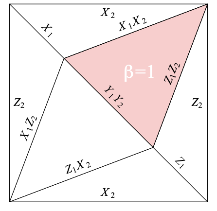
(b)

Figure 3.1: Examples of classifying spaces taken from Okay et al. [ORBR17]. (a) is the GHZ proof, (b) Mermin’s square.

For any closed set of Weyl operators Okay et al. defines a topological space (Figure 3.1). They show that key properties of the set of operators are reflected in the topology of this space. One of their results is that both state-dependent and state-independent contextuality can be detected by the non-vanishing of a cohomology class. Recall that each $n$-qudit Weyl operator $W(p_{1},p_{2})\neq I$ has $d$ distinct eigenvalues $\omega^{0},\dots,\omega^{d-1}$. Under the identification $\omega^{i}\mapsto i$ each Weyl operator defines a projective measurement with outcomes $\mathbb{Z}_{d}$. A state-dependent or state-independent contextuality proof is a proof that either the state-dependent or state-independent empirical models

$$\mathcal{S}_{\mathcal{O}}:(\mathcal{O},\mathcal{M},\mathbb{Z}_{d}),\quad\mathcal{S}_{\mathcal{O},\psi}:(\mathcal{O},\mathcal{M},\mathbb{Z}_{d})$$ (3.3)

are contextual.

In this chapter, we consider the following problem. What is the minimal structure required to define the topological obstruction at the level of empirical models. Secondly, assuming that the topological obstruction can be defined, are there instances where the Čech cohomology obstruction vanishes, but the topological obstruction does not?

3.0.1 Structure of chapter

In Section 3.1 we introduce bundles over commutative partial monoids and we prove the splitting lemma, relating left splittings, right splittings, and trivialisations. In Section 3.2 we define the cohomology of a commutative partial monoid. We show that the problem extending a local right splitting of a bundle is characterised by a cohomological obstruction. In Section 3.3 we introduce a class of measurement scenarios and empirical models generalising closed sets of Weyl operators. We show that for any such empirical model a cohomological obstruction can be defined. Finally, in Section 3.4 we show that this obstruction is not stronger than the Čech cohomology obstruction.

3.1 Bundles over commutative partial monoids

In this chapter, we are working with commutative groups, monoids, and partial monoids. We will therefore ommit the word commutative to avoid unnecessarily complicating terminology.

Recall that if $G$ and $H$ are groups then a group extension of $H$ by $G$ is a sequence of groups and homomorphisms

(3.4)

such that $i$ is injective, $j$ is surjective, and $\text{im}(i)=\text{ker}(j)$. The simplest example of a group extension of $H$ by $G$ is the product $G\times H$ along with the inclusion $\text{in}_{1}:G\to G\times H$ and the projection $\pi_{2}:G\times H\to H$.

(3.5)

As a group extension, the direct product is not interesting because its structure is determined completely by $G$ and $H$. It is therefore called the trivial extension. A homomorphism $h:G\to G\times K$ that is compatible with both the inclusion and projection maps, that is the diagram

(3.6)

commutes is called a trivialisation. It can be shown that any trivialisation is an isomorphism. A bundle that has a splitting is said to split, and its structure is therefore also determined completely by $G$ and $K$. The splitting lemma for groups gives a necessary and sufficient characterisation of when a group extension has a splitting.

Partial monoids generalise groups by omitting the requirement that elements have inverses, and the requirement that all products are defined.

Definition 3.1.1.

A (commutative) partial monoid is a tuple $(M,+,0)$ where $M$ is a set, the product $+:M^{2}\to M$ is a partial function, and $0\in M$ is the identity, such that the following conditions hold:

• Commutativity: $m+m^{\prime}$ is defined if and only if $m^{\prime}+m$ is defined and $m+m^{\prime}=m^{\prime}+m$, for all $m,m^{\prime}\in M$.

• Identity: $0+m$ is defined and $0+m=m$ for all $m\in M$.

• Associativity: For all $m,m^{\prime},m^{\prime\prime}\in M$

  • If $(m+m^{\prime})+m^{\prime\prime}$ and $m+(m^{\prime}+m^{\prime\prime})$ are both defined then they are equal.

  • If $m+m^{\prime},m+m^{\prime\prime},m^{\prime}+m^{\prime\prime}$ are all defined then $(m+m^{\prime})+m^{\prime\prime}$ and $m+(m^{\prime}+m^{\prime\prime})$ are both defined.

If the product $+$ is a total function then $(M,+,0)$ is a commutative monoid.

In this section, we introduce a generalisation of group extensions to partial monoids and we show that the splitting lemma generalises, and the problem of extending a local splitting to a global splitting is equivalent.

3.1.1 Bundles

To generalise the definition of a group extension to partial monoids we first recast the definition to emphasise the role of a group action.

Definition 3.1.2.

Let $\theta:G\times X\to X$ be a group action. $\theta$ is free if $\theta(\_,x):G\to X$ is injective for all $x\in X$. The orbit of $x\in X$, is the set of elements that are equivalent to $x$ up to the action of $G$:

$$[x]_{\theta}:=\{\theta(g,x)\mid g\in G\}$$ (3.7)

We write $X/\theta$ for the set of orbits. When a particular group action is assumed we will simplify notation by defining $g\cdot x:=\theta(g,x)$.

Observe that for any group extension there is an action of $G$ on $H$ defined by

$$\theta:G\times H\to H::(g,h)\mapsto i(g)+_{H}h$$ (3.8)

This action is free because $i$ is injective and $H$ has inverses. It is also compatible with the group structures of $G$ and $H$ in the sense that it is a homomorphism from $G\times H$ to $H$. The requirement that $\text{im}(i)=\text{ker}(j)$ is equivalent to saying that the orbits of $\theta$ and the fibers of $j$ are the same:

$$H/\theta=\{j^{-1}(k)\mid k\in K\}$$ (3.9)

We can recast the definition of a group extension in terms of this action. A group extension can be defined as a surjective homomorphism $j:H\to K$ and a free, compatible group action $\theta$ such that the orbits of $\theta$ are the fibers of $j$. We will use this view of group extensions to generalise them to partial monoids.

For a partial monoid the natural notion of homomorphism is a function on the underlying set that preserves the identity and products whenever they are defined.

Definition 3.1.3.

A homomorphism of partial monoids $h:M\to M^{\prime}$ is a function between the underlying sets, such that:

• $h$ preserves the identity element: $h(0_{M})=0_{M^{\prime}}$.

• $h$ preserves products: $h(m_{1})+_{M^{\prime}}(m_{2})$ is defined and $h(m_{1}+_{M}m_{2})=h(m_{1})+_{M^{\prime}}h(m_{2})$, for all $m_{1},m_{2}$ such that $m_{1}+_{M}m_{2}$ is defined.

If $G$ is a group and $M$ is a partial monoid then the set product $G\times M$ is a partial monoid with identity and product defined component-wise.

$$0_{G\times M} =(0_{G},0_{M})$$ (3.10)

$$(g,m)+_{G\times M}(g^{\prime},m^{\prime}) =(g+_{A}g^{\prime},m+_{M}m^{\prime})$$ (3.11)

for all $g,g^{\prime}\in G$ and $m,m^{\prime}\in M$ such that $m+_{M}m^{\prime}$ is defined. We define an action of a group $G$ on $M$ to be a group action, in the usual sense, that is furthermore a homomorphism from $G\times M$ to $M$.

Definition 3.1.4.

Let $G$ be a group and $M$ a partial monoid. An action of $G$ on $M$ is a homomorphism $\theta:G\times M\to M$ such that the following conditions hold:

$$\theta(0,\_) =\text{id}_{M}$$ (3.12)

$$\theta(g,\_)\circ\theta(g^{\prime},\_) =\theta(g+g^{\prime},\_),\quad\text{for all $g,g^{\prime}\in G$}$$ (3.13)

We define a bundle over a partial monoid to be a partial monoid equipped with a compatible group action and a surjective homomorphism such that the fibers of the homomorphism and the orbits of the action are the same.

Definition 3.1.5.

Let $G$ be a group and $M$ a partial monoid. A $G$-bundle over $M$ is a tuple $(N,j,\theta)$, where

• $N$ is a partial monoid,

• $\theta:G\times N\to N$ is a free action,

• $j:N\to M$ is a surjective homomorphism,

such that the orbits of $\theta$ are the fibers of $j$:

$$N/\theta=\{j^{-1}(m)\mid m\in M\}$$ (3.14)

$\theta$ is called the bundle action and $j$ the bundle map.

The simplest example of a $G$-bundle over $M$ is given by the product $G\times M$. Write $\theta_{G\times M}$ for the action of $G$ on $G\times M$ applying the group operation of $G$ on the first component, and $\pi_{2}:G\times M\to M$ for the projection onto the second component.

$$\theta(g,(g^{\prime},m)):=(g+g^{\prime},m)$$ (3.15)

The triple $(G\times M,\theta_{G\times M},\pi_{2})$ is called the trivial bundle. As a bundle it has no interesting structure because it is completely determined by $G$ and $M$ alone.

3.1.2 The splitting lemma

Let be a group extension. The splitting lemma for groups gives the following characterisation of trivialisations, that is homomorphisms $h:H\to G\times K$ such that the following diagram commutes:

(3.16)

in other words, $\text{in}_{1}=h\circ i$ and $j=\pi_{2}\circ h$. Trivialisations are necessarily isomorphisms. Any group extension that has a trivialisation is therefore isomorphic to the product group extension.

A left splitting is a homomorphism $s:H\to G$ such that $i\circ l=\text{id}_{H}$. A right splitting a homomorphism $r:K\to H$ such that $r\circ j=\text{id}_{K}$. The splitting lemma for groups states that the three are equivalent: A group extension has a left splitting if and only if it has a right splitting, if and only if it has a trivialisation.

To generalise left splittings and trivialisations we observe that their definitions can be recast in terms of the group action of $G$ on $H$.

Definition 3.1.6.

Let $G$ be a group, $M,M^{\prime}$ partial monoids, and $\theta:G\times M\to M$, $\theta^{\prime}:G\times M^{\prime}\to M^{\prime}$ group actions. An action homomorphism $h:\theta\to\theta^{\prime}$ is a partial monoid homomorphism $h:M\to M^{\prime}$ such that $\theta^{\prime}(g,f(x))=f(\theta(g,x))$ for all $g\in G,x\in X$.

For any group $G$ write write $\theta_{G}$ for the group action of $G$ on itself: $\theta_{G}(g,g^{\prime}):=g+_{G}g^{\prime}$. A left splitting of a group extension is then equivalently an action homomorphism from the bundle action $\theta$ to $\theta_{G}$. The requirement that a trivialisation is compatible with the inclusion maps, that is $\text{in}_{1}=h\circ i$ is equivalent to $h$ being an action homomorphism from the bundle action $\theta$ to the bundle action on the product bundle $\theta_{G\times M}$.

Definition 3.1.7.

Let $G$ be a group, $M$ a partial monoid, and $B=(N,j,\theta)$ a $G$-bundle over $M$.

1. A left splitting is an action homomorphism $l:\theta\to\theta_{G}$.

2. A right splitting is a partial monoid homomorphism $r:M\to N$ such that $j\circ r=\text{id}_{M}$.

3. A trivialisation is an action homomorphism $h:\theta\to\theta_{G\times M}$ such that $j=\pi_{2}\circ h$.

For example, the trivial bundle $(G\times M,\theta_{G\times M},\pi_{2})$ has a left splitting $\pi_{1}$ and a right splitting $\text{in}_{2}$:

$$\pi_{1}:G\times M\to G ::(g,m)\mapsto b$$ (3.17)

$$\text{in}_{2}:M\to G\times M ::=m\mapsto(0_{B},m)$$ (3.18)

Let $B=(N,j,\theta)$ be a $G$-bundle over a partial monoid $M$ and let $l:N\to G$ be a left splitting. There is then a natural map from $N$ to $G\times M$ given by

$$\langle l,j\rangle:N\to G\times M::=n\mapsto(l(n),j(n))$$ (3.19)

Because $l$ is a left splitting and therefore an action homomorphism from $\theta$ to $\theta_{G}$ we have that $\langle l,j\rangle$ is an action homomorphism from $\theta$ to the bundle action $\theta_{G\times M}$ of the trivial bundle. $\langle l,j\rangle$ is a trivialisation.

We then clearly have $\pi_{2}\circ\langle l,j\rangle=j$. Because $l$ is an action homomorphism from $\theta$ to $\theta_{G}$ we have that $\langle l,j\rangle$ is an action homomorphism from $\theta$ to $\theta_{G\times M}$. Conversely if $h:N\to G\times M$ is a trivialisation then we can define a left splitting by projecting onto the first component: $\pi_{1}\circ h$.

Because the bundle action $\theta$ is free something similar is true for right splittings. For any left splitting $l$ let $\mathcal{R}(l)$ be the function

$$\mathcal{R}(l):M\to N::=m\mapsto-l(\eta(m))\cdot\eta(m)$$ (3.20)

where $\eta:M\to N$ is any function such that $j\circ\eta=\text{id}_{M}$. Observe that the definition is independent of the choice of $\eta$ because

$$-l(g\cdot\eta(m))\cdot(g\cdot\eta(m)) =(-l(\eta(m))-g+g)\cdot\eta(m)$$ (3.21)

$$=-l(\eta(m))\cdot\eta(m)$$ (3.22)

for any $m\in M$ and $g\in G$.

Lemma 3.1.1 (Splitting lemma).

Let $B=(N,\theta,j)$ be a $G$-bundle over a partial monoid $M$.

1. The map $l\mapsto<l,j>$ is a bijection between left splittings and trivialisations.

2. The map $l\mapsto\mathcal{R}(l)$ is a bijection between left and right splittings.

Proof.

1. $h\mapsto\pi_{1}\circ h$ is an inverse to $l\mapsto<l,j>$. $\pi_{1}\circ h$ is an action homomorphism from $\theta$ to $\theta_{G}$ if and only if $h$ is an action homomorphism from $\theta$ to $\theta_{G\times M}$.

For 2. we first check that $\mathcal{R}(l)$ is a homomorphism. It preserves the identity. We have $\eta(0)=a\cdot 0$ for some unique $a$. Hence $\mathcal{R}(l)(0)=(-l(\eta(0)))\cdot\eta(0)=-l(a\cdot 0)\cdot(a\cdot 0)=(0-a+a)\cdot 0$ as required. To see that it preserves products, take $m,m^{\prime}$ such that $m+_{M}m^{\prime}$ is defined. There is a unique $g$ such that $\eta(m+m^{\prime})=g\cdot(\eta(m)+\eta(m^{\prime}))$. Therefore

$$\mathcal{R}(l)(m+m^{\prime}) =(-l(\eta(m+m^{\prime})))\cdot\eta(m+m^{\prime})$$ (3.23)

$$=(-l(g\cdot(\eta(m)+\eta(m^{\prime})))\cdot(g\cdot(\eta(m)+\eta(m^{\prime})))$$ (3.24)

$$=(-l(\eta(m))-l(\eta(m^{\prime}))-g+g)\cdot(\eta(m)+\eta(m^{\prime}))$$ (3.25)

$$=\mathcal{R})(l)(m)+\mathcal{R}(l)(m^{\prime})$$ (3.26)

To see that $\mathcal{R}$ is a bijection we can define the inverse directly as follows. For any right splitting $r:M\to N$ there is a unique function $\mathcal{R}^{-1}(r):M\to N$ such that

$$\mathcal{R}^{-1}(r)(n)\cdot n=r(j(n))$$ (3.27)

for all $n\in N$.

We first check that it is a homomorphism. For the identity we have $h(j(0))=0$ and $h(j(0))=s(0)\cdot 0$, hence $s(0)=0$ as required. That it preserves products we have both

$$h(j(n+n^{\prime}))=s(n+n^{\prime})\cdot(n+n^{\prime})$$ (3.28)

and

$$h(j(n+n^{\prime})) =h(j(n))+h(j(n^{\prime}))$$ (3.29)

$$=s(n)\cdot n+s(n^{\prime})\cdot n^{\prime}$$ (3.30)

$$=(s(n)+s(n^{\prime}))\cdot(n+n^{\prime})$$ (3.31)

Therefore, by uniqueness of $s$ we have $s(n+n^{\prime})=s(n)+s(n^{\prime})$. Finally to see that it preserves the action, we have $r(j(g\cdot n))=r(j(n))$. Hence

$$\mathcal{R}^{-1}(r)(g\cdot n)\cdot(g\cdot n)=\mathcal{R}^{-1}(r)(n)\cdot n$$ (3.32)

$\mathcal{R}^{-1}(r)(g\cdot n)=g+\mathcal{R}^{-1}(r)(n)$

Finally we check that $\mathcal{R}^{-1}$ in fact is an inverse to $\mathcal{R}$.

$$R_{B}(R_{B}^{-1}(r)) =m\mapsto(-s_{r}(\eta(m)))\cdot\eta(n)$$ (3.33)

$$=m\mapsto r(j(\eta(m)))=m\mapsto r(m)$$ (3.34)

and

$$(h^{-1}\circ\text{in}_{M})(j(n)) =h^{-1}(0,j(n))$$ (3.35)

$$=(0-h_{1}(n))\cdot n$$ (3.36)

Hence by uniqueness $(h^{-1}\circ\text{in}_{M})\mapsto h$ and so $\mathcal{R}$ is a left inverse to $\mathcal{R}^{-1}$. ∎

Similarly, as for groups, trivialisations of bundles are necessarily isomorphisms. The splitting lemma, therefore, gives a characterisation of when a bundle is isomorphic to the trivial bundle. A natural candidate for the inverse of a trivialisation $h$ is the map given by first taking the left splitting $\pi_{1}\circ h:N\to G$, then composing the right splitting associated with $\pi_{1}\circ h$ with the projection $\pi_{2}$: $\mathcal{R}(\pi_{1}\circ h)\circ\pi_{2}$. It can be verified that this map in fact is an inverse.

Lemma 3.1.2.

Trivialisations are isomorphisms. Let $B=(N,j,\theta)$ be an $A$-bundle over a commutative partial monoid $M$ and $h:N\to A\times M$ a trivialisation. The inverse of $h$ is

$$h^{-1}:A\times M\to N::=(a,m)\mapsto(a-h_{1}(\eta(m)))\cdot\eta(m)$$ (3.37)

where $\eta:\prod_{m\in M}j^{-1}(m)$ is an arbitrary section and $h_{1}=\text{proj}_{1}\circ h:N\to A$ is the first component of $h$.

Proof.

We first show that $h^{-1}$ is independent of the choice of the section $\eta$. Any other section $\eta^{\prime}=m\mapsto\gamma(m)\cdot\eta(m)$ differs from $\eta$ by some $\gamma:M\to A$. If we expand the definition of $h^{-1}$ using the section $\eta^{\prime}$ in terms of $\gamma$ and $\eta$ we see that the terms involving $\gamma$ cancels out. For any $m\in M$ we have

$$(a-h_{1}(\eta^{\prime}(m)))\cdot\eta^{\prime}(m) =(a-h_{1}(\gamma(m)\cdot\eta(m)))\cdot(\gamma(m)\cdot\eta(m))$$ (3.38)

$$=(a-\gamma(m)-h_{1}(\eta(m))+\gamma(m))\cdot\eta(m)$$ (3.39)

$$=(a-h_{1}(\eta(m)))\cdot\eta(m)$$ (3.40)

Therefore $h^{-1}$ is independent of the choice of $\eta$.

Next, we check that $h^{-1}$ is a left inverse to $h$. Let $n\in N$. To see that $h^{-1}(h(n))=n$ we first expand $h(n)=(h_{1}(n),h_{2}(n))$ into the two components of the product. Using the section $\eta$ we can write $n$ uniquely on the form

$$n=a\cdot\eta(m)$$ (3.41)

where $a\in A$ and $m=j(n)$. Because $h$ is a trivialisation $j(n)=h_{2}(n)$.

$$h^{-1}(h(n)) =h^{-1}(h_{1}(n),h_{2}(n))$$ (3.42)

$$=h^{-1}(h_{1}(n),m)$$ (3.43)

Because both $h$ and $\text{proj}_{1}$ preserve the action of $A$ we have $h_{1}(a\cdot\eta(m))=a+h_{1}(\eta(m))$ therefore if we plug $(h_{1}(n),m)$ into $h^{-1}$ the terms involving $h_{1}(\eta(m))$ cancels out

$$h^{-1}(h_{1}(n),m) =(h_{1}(n)-h_{1}(\eta(m)))\cdot\eta(m)$$ (3.44)

$$=(h_{1}(a\cdot\eta(m))-h_{1}(\eta(m)))\cdot\eta(m)$$ (3.45)

$$=(a+h_{1}(\eta(m))-h_{1}(\eta(m)))\cdot\eta(m)$$ (3.46)

$$=a\cdot\eta(m)=n$$ (3.47)

as required.

Finally, we check that $h^{-1}$ is a right inverse to $h$. Let $(a,m)\in A\times M$. We first expand the definition of $h^{-1}(a,m)$

$$h(h^{-1}(a,m)) =h((a-h_{1}(\eta(m)))\cdot\eta(m))$$ (3.48)

and then separately check that $h_{1}(h^{-1}(a,m))=a$ and $h_{2}(h^{-1}(a,m))_{2}=m$. For the first part we use the fact that $h_{1}$ is an $A$-action homomorphism

$$h_{1}((a-h_{1}(\eta(m)))\cdot\eta(m))=(a-h_{1}(\eta(m)))+h_{1}(\eta(m))=a$$ (3.49)

The second part follows because $h$ maps the fiber $j^{-1}(m)$ to $A\times\{m\}$

$$h_{2}((a-h_{1}(\eta(m)))\cdot\eta(m))=m$$ (3.50)

as required. ∎

3.1.3 Extending local splittings

The splitting lemma gives a correspondence between left splittings, right splittings, and trivialisations. We now show that this correspondence is compatible with restrictions. This means that the problem of extending a right splitting, left splitting, or trivialisations defined on a sub-bundle are all equivalent.

Suppose that $B=(N,j,\theta)$ is a $G$-bundle over a partial monoid $M$, and that $M^{\prime}\subset M$ is a sub partial monoid. We first explain that $B$ restricts to a sub bundle over $M^{\prime}$.

The pre-image $j^{-1}(M^{\prime})\subset N$ is a sub-partial monoid of $N$, and it is closed under the action $\theta$. We can therefore restrict $B$ to a $G$-bundle over $M^{\prime}$ by restricting both the bundle map $j$ and action $\theta$.

Definition 3.1.8.

Let $B=(N,j,\theta)$ be a $G$-bundle over a partial monoid $M$ and $M^{\prime}\subset M$ a sub partial monoid. The restriction of $B$ to $M^{\prime}$, denoted by $B\rvert_{M^{\prime}}$, is the $G$-bundle over $M^{\prime}$

$$B\rvert_{M^{\prime}}:=\big{(}N^{\prime},j^{\prime},\theta^{\prime}\big{)}$$ (3.51)

where $N^{\prime}:=j^{-1}(M^{\prime})$ and $j^{\prime}:N^{\prime}\to M^{\prime},\theta^{\prime}:G\times N^{\prime}\to N^{\prime}$ are the restrictions of $j$ and $\theta$ to $N^{\prime}$.

Because the maps in the splitting lemma are defined pointwise they are natural with respect to restrictions. The problems of extending a left splitting, right splitting, or trivialisation of the restricted bundle $B\rvert_{M^{\prime}}$ to $B$ are therefore equivalent.

Lemma 3.1.3.

Let $B=(N,j,\theta)$ be a $G$-bundle over a partial monoid $M$, $M^{\prime}\subset M$ a sub partial monoid, and $l^{\prime}:M^{\prime}\to G$ a left splitting of the restricted bundle $B\rvert_{M^{\prime}}$. The following conditions are equivalent:

• There exists a left splitting $l:N\to G$ such that $l\rvert_{M^{\prime}}=l^{\prime}$.

• There exists a trivialisation $h:N\to G\times M$ such that $h\rvert_{N^{\prime}}=<l^{\prime},j>$.

• There exists a right splitting $r:M\to N$ such that $r\rvert_{M^{\prime}}=\mathcal{R}(l^{\prime})$.

3.2 Cohomology of commutative partial monoids

We concluded the previous section by explaining that for a $G$-bundle $B$ over a partial monoid $M$ the problems of extending either a left splitting, right splitting, or trivialisation, defined on a sub bundle are equivalent. In this section we show that this problem can be given a cohomological characterisation. The construction can be seen as a generalisation of group cohomology.

Let $G$ and $K$ be groups. A well-known problem in group theory is to classify the possible group extensions of $K$ by $G$. An elegant solution to this problem is given by group cohomology [Bro12]. Two group extensions are equivalent if they are related by an isomorphism:

(3.52)

So in particular an extension splits if it is equivalent to the trivial extension.

For any group $K$ there is a topological space $X_{K}$ called the classifying space of $K$. There is a bijection between the second cohomology group $H^{2}(X_{K},G)$ of $X_{K}$ with coefficients in $G$ , and equivalence classes of group extensions. In particular, the equivalence class of the trivial extension correspond to the zero class $0\in H^{2}(X_{K};G)$.

In this section, we first generalise group cohomology. In Section 3.2.1 we define the relative cohomology groups $H^{n}(M,M^{\prime};G)$ of a partial monoid $M$ with respect to a sub partial monoid $M\subset M^{\prime}$ with coefficients in a group $G$. In 3.2.2 we define for any local right splitting $r$ of a sub-bundle a cohomological obstruction $\mu(r)\in H^{2}(M,M^{\prime};G)$ and we show that $\mu(r)=0$ if and only if $r$ can be extended to a global splitting.

3.2.1 The cohomology groups of a partial monoid

Let $G$ be a group, $M$ a partial monoid, and $M^{\prime}\subset M$ a sub partial monoid. In this section, we define the relative cohomology groups $H^{n}(M,M^{\prime};G)$.

We begin by defining a family of sets $\{M_{n}\}_{n\in\mathbb{N}}$ and boundary maps $\delta_{n,i}:M_{n}\to M_{n-1}$, where $i=1,\dots,n$ encoding the structure of a partial monoid $M$.

Definition 3.2.1.

Let $K$ be a commutative partial monoid. $\{K_{n}\}_{n\geq 0}$ and $\delta_{n,i}:K_{n}\to K_{n-1}$, where $n\geq 1,i=0,\dots,n$ are defined by $K_{0}:=\{()\}$ and when $n\geq 1$

$$K_{n} :=\{(k_{1},k_{2},\cdots,k_{n})\in K^{n}\mid k_{1}+k_{2}+\cdots+k_{n}\text{ is defined}\}$$ (3.53)

$$\delta_{n,i} ::=(k_{1},\dots,k_{n})\mapsto(k_{1},\dots,k_{i-1},k_{i}+k_{i+1},k_{i+2},\dots,k_{n})$$ (3.54)

By considering the set of functions $f:M_{n}\to G$ that vanish on $M^{\prime}_{n}\subset M_{n}$ we define the relative co-chain complex

(3.55)

Definition 3.2.2.

Let $G$ be a group, $M$ a partial monoid, and $M^{\prime}\subset M$ a sub partial monoid.

1. The relative $n$-cochains, denoted by $C^{n}(M,N;G)$, is the commutative group of assignments $f:M_{n}\to G$ that vanish on $M^{\prime}_{n}$.

   $$C^{n}(M^{\prime},M;G) :=\{f:M_{n}\to G\mid f\rvert_{{M^{\prime}}_{n}}=0\}$$ (3.56)

2. The $n$’th coboundary map, denoted by $d^{n}$ is the following homomorphism from the relative $n$-cochains to relative $(n-1)$-cochains

   $$d^{n} :C^{n}(M^{\prime},M;G)\to C^{n+1}(M^{\prime},M;G)$$ (3.57)

   $$d^{n}(f) :=(m_{1},\dots,m_{n})\mapsto\sum_{i=0}^{n}(-1)^{i}f(\delta_{n,i}(m_{1},\dots,m_{n}))$$ (3.58)

The relative cohomology groups $H^{n}(M,M^{\prime};G)$ are the cohomology groups of this co-chain complex. To verify that this in fact defines a co-chain complex we need to verify that $d^{n+1}\circ d^{n}=0$. This can be done by a straightforward computation. In our case, it is only necessary to verify this for the maps

$$d^{2}(f)(m_{1},m_{2},m_{3}) =f(m_{2},m_{3})-f(m_{1}+m_{2},m_{3})+f(m_{1},m_{2}+m_{3})-f(m_{1},m_{2})$$ (3.59)

$$d^{1}(f)(m_{1},m_{2}) =f(m_{2})-f(m_{1}+m_{2})+f(m_{1})$$ (3.60)

$$d^{0} =0$$ (3.61)

which is easily done.

Definition 3.2.3.

Let $G$ be a commutative group $M$ a commutative partial monoid and $M^{\prime}\subset M$ a sub partial monoid.

1. The relative $n$-cocycles $Z^{n}(M,N;G):=\ker{d^{n}}$ is the kernel of $d^{n}:C^{n}(K,M;G)\to C^{n-1}(K,M;G)$.

2. The relative $n$-coboundaries is the image $B^{n}(M,N;G):=\text{im}\,d^{n-1}$ of $d^{n}:C^{n}(K,M;G)\to C^{n-1}(K,M;G)$.

3. The relative cohomology group $H^{n}(K,M;G):=Z^{n}(K,M;G)/B^{n}(K,M;G)$ is the quotient of the relative $n$-cocycles over the relative $n$-coboundaries.

3.2.2 The obstruction to extending a local splitting

Let $B=(N,\theta,j)$ be a $G$-bundle over a partial monoid $M$, $M^{\prime}\subset M$ a sub partial monoid, and $r^{\prime}:M^{\prime}\to N^{\prime}$ a right splitting of the restriction $B\rvert_{M^{\prime}}$ of $B$ to $M^{\prime}$.

To define the cohomological obstruction $\mu(r^{\prime})\in H^{2}(M,M^{\prime};G)$ we first choose a function $\eta:M\to N$, not necessarily a homomorphism, such that $j\circ\eta=\text{id}_{M}$ and $\eta\rvert_{M^{\prime}}=r^{\prime}$. $\eta$ is not necessarily a homomorphism but because $j\circ\eta=\text{id}_{M}$ there is for every $m_{1},m_{2}\in M$ some $g\in G$ such that $\eta(m_{1}+_{M}m_{2})=g\cdot(\eta(m_{1})+_{M}\eta(m_{2}))$. Because $\theta$ is free this $g$ is unique.

Definition 3.2.4.

Let $B=(N,j,\theta)$ be an $G$-bundle over a partial monoid $M$, $M^{\prime}\subset M$ a sub partial monoid, and $\eta:M\to N$ a function such that $\eta\circ j=\text{id}_{M}$. Write $\Delta\eta:M_{2}\to G$ for the unique function satisfying

$$\eta(m_{1}+m_{2})=\Delta\eta\,(m_{1},m_{2})\cdot(\eta(m_{1})+\eta(m_{2}))$$ (3.62)

for all $(m_{1},m_{2})\in M_{2}$.

$\Delta\eta$ can be thought of as measuring the failure of $\eta$ to be a splitting because $\eta$ is a homomorphism if and only if $\Delta\eta=0$. We define $\mu(r^{\prime})$ to be the cohomology class of $\Delta\eta$.

Definition 3.2.5.

Let $B=(N,j,\theta)$ be an $G$-bundle over $M$, $M^{\prime}\subset M$ a sub-partial monoid, and $r^{\prime}:M^{\prime}\to N^{\prime}$ a right splitting of $B\rvert_{M^{\prime}}$. The obstruction to $r^{\prime}$, is the cohomology class

$$\mu(r^{\prime}):=[\Delta\eta]\in H^{2}(M^{\prime},M^{\prime};A)$$ (3.63)

where $\eta:M\to N$ is any function such that $\eta\rvert_{M^{\prime}}=r^{\prime}$ and $j\circ\eta=\text{id}_{M}$.

For this to be well defined we need to check that $\Delta\eta$ is a relative co-cycle and that the cohomology class $[\Delta\eta]$ is independent of the choice of $\eta$.

Lemma 3.2.1.

Let $B=(N,j,\theta)$ be an $A$-bundle over a commutative partial monoid $M$, $M^{\prime}\subset M$ a sub partial monoid, and $r$ a right splitting of the restricted bundle $B\rvert_{M^{\prime}}$.

1. $\Delta\eta\in Z^{2}(M^{\prime},M;A)$ for any $\eta:M\to N$ such that $\eta\rvert_{M^{\prime}}=r^{\prime}$ and $j\circ\eta=\text{id}_{M}$.

2. $(\Delta\eta-\Delta\eta^{\prime})\in B^{2}(M^{\prime},M;A)$ for any two $\eta,\eta^{\prime}:M^{\prime}\to N^{\prime}$ such that $\eta\rvert_{M^{\prime}}=\eta^{\prime}\rvert_{M^{\prime}}=r^{\prime}$ and $j\circ\eta=j\circ\eta^{\prime}=\text{id}_{M}$.

Proof.

For 1. we first have to show that $\Delta\eta$ is a relative cochain, that is, that $\Delta\eta$ vanishes on $(M_{2}^{\prime})$, and secondly that

$$\Delta\eta\,(m_{2},m_{3})-\Delta\eta\,(m_{1}+m_{2},m_{3})+\Delta\eta\,(m_{1},m_{2}+m_{3})-\Delta\eta\,(m_{1},m_{2})=0$$ (3.64)

for all $(m_{1},m_{2},m_{3})\in M_{3}$. That $\Delta\eta$ vanishes on $M_{2}^{\prime}$ is clear because its restriction is a homomorphism. For the second part we use that $m_{1}+m_{2}+m_{3}$ can be written as both $m_{1}+(m_{2}+m_{3})$ and $(m_{1}+m_{2})+m_{3}$.

$$\eta(m_{1}+(m_{2}+m_{3})) =\Delta\eta\,(m_{1},m_{2}+m_{3})\cdot(\eta(m_{1})+\eta(m_{2}+m_{3}))$$

$$=(\Delta\eta\,(m_{1},m_{2}+m_{3})+\Delta\eta\,(m_{2},m_{3}))\cdot(\eta(m_{1})+\eta(m_{2})+\eta(m_{3}))$$

and similarly

$$\eta((m_{1}+m_{2})+m_{2}) =(\Delta\eta\,(m_{1}+m_{2},m_{3})+\Delta\eta\,(m_{1},m_{2}))\cdot(\eta(m_{1})+\eta(m_{2})+\eta(m_{3}))$$

Because the two terms are equal and the action is free

$$\Delta\eta\,(m_{1},m_{2}+m_{3})+\Delta\eta\,(m_{2},m_{3})=\Delta\eta\,(m_{1}+m_{2},m_{3})+\Delta\eta\,(m_{1},m_{2})$$ (3.65)

as required.

For 2. suppose that $\eta,\eta^{\prime}$ are two sections that extend $r$. We have to show that there is some $\gamma:C^{1}(M^{\prime},M;A)$ such that

$$\Delta\eta\,(m_{1},m_{2})-\Delta\eta^{\prime}\,(m_{1},m_{2})=\gamma(m_{1})-\gamma(m_{1}+m_{2})+\gamma(m_{2})$$ (3.66)

for all $(m_{1},m_{2})\in M_{2}$. Let $\gamma:M\to A$ be the unique function such that

$$\eta=m\mapsto s(m)\cdot\eta^{\prime}(m)$$ (3.67)

Because $\eta,\eta^{\prime}$ both extend $r$ we have $s\rvert_{M^{\prime}}=0$ and so $\gamma$ is a relative cochain, $\gamma\in C^{1}(M^{\prime},M;A)$. Expanding $\eta(m_{1}+m_{2}),\eta(m_{1}),\eta(m_{2})$ in terms of $\gamma$ and $\eta^{\prime}$ gives

$$\eta(m_{1}+m_{2}) =\Delta\eta\,(m_{1},m_{2})\cdot(\eta(m_{1})+\eta(m_{2}))$$ (3.68)

$$=(\Delta\eta\,(m_{1},m_{2})+s(m_{1})+s(m_{2}))\cdot(\eta^{\prime}(m_{1})+\eta^{\prime}(m_{2}))$$ (3.69)

and

$$\eta(m_{1}+m_{2}) =s(m_{1}+m_{2})\eta^{\prime}(m_{1}+m_{2})$$ (3.70)

$$=(s(m_{1}+m_{2})+\Delta\eta^{\prime}\,(m_{1},m_{2}))\cdot(\eta^{\prime}(m_{1})+\eta^{\prime}(m_{2}))$$ (3.71)

hence

$$\Delta\eta\,(m_{1},m_{2})+s(m_{1})+s(m_{2})=s(m_{1}+m_{2})+\Delta\eta^{\prime}\,(m_{1},m_{2})$$ (3.72)

as required. ∎

Observe that the obstruction is sound in the sense that if $r^{\prime}$ can be extended to a right splitting $r:M\to N$ then $[\Delta\eta]=0$. This is true because if such an $r$ exists then the cohomology class $[\Delta\eta]$ is equal to the cohomology class $[\Delta r]$ had we instead chosen $r$. Because $r$ is a homomormphism $\Delta r=0$ and so $[\Delta r]=0$ as required.

We now show that the obstruction in fact is complete in the sense that $\mu(r^{\prime})=0$ if and only if $r^{\prime}$ can be extended globally.

Theorem 3.2.1.

Let $B=(N,j,\theta)$ be a $G$-bundle over a partial monoid $M$, $M^{\prime}\subset M$ a sub partial monoid, and $r$ a right splitting of $B\rvert_{M^{\prime}}$. There exists a right splitting $r:M\to N$ such that $r\rvert_{M^{\prime}}=r^{\prime}$ if and only if $\mu(r^{\prime})=0$.

Proof.

We have already explained that $\mu(r^{\prime})=0$ if $r^{\prime}$ can be extended globally. For the converse suppose that $\mu(r^{\prime})=0$.

We extend $r^{\prime}$ to a global right splitting $r:M\to N$ by first choosing a function $\eta:M\to N$ such that $\eta\circ j=\text{id}_{M}$ and $\eta\rvert_{M^{\prime}}=r^{\prime}$. Because $[\Delta\eta]=0$ there is a unique $\gamma\in C^{1}(M^{\prime},M;A)$ such that $\Delta\eta=d^{1}(\gamma)$. We define $r$ by

$$r(m)::=-\gamma(m)\cdot\eta(m)$$ (3.73)

for all $m\in M$. To see that $r$ is a homomorphism take $m_{1},m_{2}\in M$ such that $m_{1}+_{M}m_{2}$ is defined. We have

$$r(m_{1}+m_{2}) =-\gamma(m_{1}+m_{2})\cdot\eta(m_{1}+m_{2})$$ (3.74)

$$\eta(m_{1}+m_{2}) =\Delta\eta\,(m_{1},m_{2})\cdot(\eta(m_{1})+\eta(m_{2}))$$ (3.75)

$$\Delta\eta\,(m_{1},m_{2}) =d^{1}(\gamma)(m_{1},m_{2})=\gamma(m_{1})-\gamma(m_{1}+m_{2})+\gamma(m_{2})$$ (3.76)

Hence

$$r(m_{1}+m_{2}) =-\gamma(m_{1}+m_{2})\cdot\eta(m_{1}+m_{2})$$ (3.77)

$$=(-\gamma(m_{1}+m_{2})+\Delta\eta\,(m_{1},m_{2}))\cdot(\eta(m_{1})+\eta(m_{2}))$$ (3.78)

$$=(-\gamma(m_{1}+m_{2})+\gamma(m_{1})-\gamma(m_{1}+m_{2})+\gamma(m_{2}))\cdot(\eta(m_{1})+\eta(m_{2}))$$ (3.79)

$$=r(m_{1})+r(m_{2})$$ (3.80)

as required. ∎

3.3 Measurement scenarios with bundle structure

We now introduce a class of measurement scenarios and empirical models generalising the state-dependent and state independent empirical models $\mathcal{S}_{\mathcal{O}},\mathcal{S}_{\mathcal{O},\psi}:(\mathcal{O},\mathcal{M},\mathbb{Z}_{d})$ associated with a closed set of Weyl operators $\mathcal{O}\subset P_{n,d}$ and a state $\psi$. We first give an abstract description of the structure of these models. In Section 3.3.1 we explain that for models of this type a test for (non) contextuality is to extend a local homomorphism to a global homomorphism. We give two examples, based on GHZ and Mermin’s square. In Section 3.3.2 we show that these scenarios can be given a bundle structure, and that the cohomological obstruction to extending local splittings can be used to detect contextuality.

Let $\mathcal{O}\subset P_{n,d}$ be a closed set of Weyl operators. $\mathcal{O}$ contains the identity and is closed under products of commuting operators. Restricting the group product of $P_{n,d}$ to pairs of commuting operators , therefore, gives $\mathcal{O}$ the structure of a partial monoid. The set of operators $\mathcal{O}$ is also closed under the $\mathbb{Z}_{d}$-action

$$\Omega:\mathbb{Z}_{d}\times\mathcal{O}\to\mathcal{O}:=(p,O)\mapsto\omega^{p}O$$ (3.81)

where $\omega:=e^{2\pi i/d}$. Note that $\Omega$ is compatible (Definition 3.1.4) with the partial monoid product because

$$\omega^{p}O\omega^{p^{\prime}}O^{\prime}=\omega^{p+p^{\prime}}OO^{\prime}$$ (3.82)

for all $p\in\mathbb{Z}_{d}$ and commuting $O,O^{\prime}\in\mathcal{O}$.

Let $C\subset\mathcal{O}$ be a maximal context of pairwise commuting operators. $C$ is then a submonoid of $\mathcal{O}$, i.e. all products are defined. Because two operators $\omega^{q}O$ and $O$ that differ by some $\omega^{q}$ commute we also have that $C$ is closed under the action $\Omega$. Write $\Omega_{C}$ for the restriction of $\Omega$ to $C$. We now observe that any value assignment $s:C\to\mathbb{Z}_{d}$ that is consistent with quantum mechanics preserves the action $\Omega_{C}$.

Lemma 3.3.1.

Let $\mathcal{O}\subset P_{n,d}$ be a closed set of Weyl operators and $C\subset\mathcal{O}$ a maximal context. A joint outcome assignment $s:C\to\mathbb{Z}_{d}$ that is consistent with quantum mechanics is an action homomorphism (Definition 3.1.6) from $\Omega_{C}$ to the action $\theta_{\mathbb{Z}_{d}}$ of $\mathbb{Z}_{d}$ on itself.

Proof.

A measurement of a Weyl operator $M$ with outcome $q$ correspond to the $\omega^{q}$ eigenvalue. Let $s:C\to\mathbb{Z}_{d}$ be an outcome assignment and suppose that $s$ is consistent with quantum mechanics. Let $M_{1},M_{2}\in C$. There is then some state $\psi$ such that $\psi$ is an eigenvector of $M_{1},M_{2},M_{1}M_{2}$ with eigenvalues $s(M_{1}),s(M_{2}),s(M_{1}M_{2})$.

$$M_{1}\lvert\psi\rangle =\omega^{s(M_{1})}\lvert\psi\rangle$$ (3.83)

$$M_{2}\lvert\psi\rangle =\omega^{s(M_{2})}\lvert\psi\rangle$$ (3.84)

$$M_{1}M_{2}\lvert\psi\rangle =\omega^{s(M_{1}M_{2})}\lvert\psi\rangle$$ (3.85)

Using the first two equations we have

$$M_{1}M_{2}\lvert\psi\rangle=\omega^{s(M_{1})}\omega^{s(M_{2})}\lvert\psi\rangle$$ (3.87)

Comparing this to the third equations we have $s(M_{1}M_{2})=s(M_{1})+s(M_{2})$. That $s(I)=0$ is clear because $I$ only has one eigenvalue $1$ which is identified with $0$. Finally, if we multiply a Weyl operator $M$ with a scalar $\omega^{q}$, then the effect is to permute the eigenvalues, hence $s(\omega^{q}M)=q+s(M)$. ∎

From this it follows that both the state-dependent and state independent empirical models $\mathcal{S}_{\mathcal{O}},\mathcal{S}_{\mathcal{O},\psi}:(\mathcal{O},\mathcal{M}_{\mathcal{O}},\mathbb{Z}_{d})$ are instances of the following definition.

Definition 3.3.1.

Let $(X,\mathcal{M},G)$ be a measurement scenario equipped with the following additional structure:

1. The outcomes $G$ is a commutative group.

2. Each maximal context $C\in\mathcal{M}$ is a commutative monoid with a compatible action $\theta_{C}:G\times C\to C$, such that for all maximal contexts $C,C^{\prime}\in\mathcal{M}$, $g\in G$, $x,x^{\prime}\in C\cap C^{\prime}$:

   $$0_{C} =0_{C^{\prime}}$$ (3.88)

   $$x+_{C}x^{\prime} =x+_{C^{\prime}}x^{\prime}$$ (3.89)

   $$\theta_{C}(g,x) =\theta_{C^{\prime}}(g,x)$$ (3.90)

An empirical model $\mathcal{S}:(X,\mathcal{M},G)$ is an empirical model (in the usual sense), such that every local section $s\in\mathcal{S}(C)$ is an action homomorphism from $\theta_{C}$ to the action $\theta_{G}$ of $G$ on itself.

3.3.1 Detecting contextuality with homomorphisms

Suppose that $\mathcal{S}:(X,\mathcal{M},G)$ is an empirical model and measurement scenario with the additional structure of Definition 3.3.1. We first observe that the monoid structures on the contexts $C\in\mathcal{M}$ and the actions $\theta_{C}$ “glue together” to define a partial monoid and compatible action on $X$.

$$\theta(g,x) :=\theta_{C}(g,x)$$ (3.91)

$$0 :=0_{C}$$ (3.92)

$$x+x^{\prime} :=x+_{C}x^{\prime}$$ (3.93)

for any $C\in\mathcal{M}$, $x,x^{\prime}\in C$, and $g\in G$. That this is well defined follows from the compatibility conditions in Definition 3.3.1).

Note that in the case of a closed set of Weyl operators $\mathcal{O}\subset P_{n,d}$ the partial monoid structure on $\mathcal{O}$ is the structure given by gluing together the monoid structure on each maximal context. This is the case because two operators $O,O^{\prime}\in\mathcal{O}$ commute if and only if they are both contained in a maximal context $C\subset\mathcal{O}$. As a partial monoid $\mathcal{O}$ is therefore completely defined by its restriction to the maximal submonoids $C\subset\mathcal{O}$.

Because the action $\theta$ and partial monoid structure on $X$ are completely determined by the monoids and actions on the maximal contexts, it follows that $s:X\to G$ is an action homomorphism from $\theta$ to $\theta_{G}$ if and only if $s\rvert_{C}$ is an action homomorphism from $\theta_{C}$ to $\theta_{G}$ for all maximal contexts $C\in\mathcal{M}$. We can therefore consider the problem of extending a local action homomorphism $s^{\prime}\in\mathcal{S}(C)$ defined on a maximal context $C\in\mathcal{M}$ as a test for contextuality.

This test is sound, but not necessarily complete. There can be action homomorphisms $s:X\to G$ that are not global sections of $\mathcal{S}$.

We now give two examples, showing that in the case of GHZ and Mermin’s square the homomorphism condition detects contextuality.

Example 3.3.1 (Mermin’s square).

Let $X\subset P_{2}$ be any set of Pauli measurements that is closed under products of commuting measurements and contains the measurements displayed in Mermin’s square. We consider the state independent model $\mathcal{S}_{X}:(X,\mathcal{M},\mathbb{Z}_{2})$ which in this case satisfies Definition 3.3.1.

Observe that equations (1)-(6) induced by Mermin’s square all can be rearranged to be on the form

$$M_{1}\oplus M_{2}=M_{1}M_{2}$$

for $M_{1},M_{2}\in X$ with $M_{1}M_{2}=M_{2}M_{1}$. That the equations are mutually inconsistent therefore literally says that there is no homomorphism from $X$ to $\mathbb{Z}_{2}$.

GHZ is an example of state-dependent contextuality. We first show that the set of operators whose outcome when measuring a given state is deterministic is a submonoid of the total partial monoid.

Lemma 3.3.2.

Let $\mathcal{O}\subset P_{n,d}$ be a closed set of $n$-qudit Weyl operators. Let $\psi$ be a state and $\mathcal{O}_{\psi}\subset\mathcal{O}$ the subset of operators whose outcome on $\psi$ is deterministic

$$\mathcal{O}_{\psi}:=\{M\in\mathcal{O}\mid M\lvert\psi\rangle=\omega^{q}\lvert\psi\rangle,\text{ for some $q\in\mathbb{Z}_{d}$}\}$$ (3.94)

$\mathcal{O}_{\psi}$ is a sub monoid of $\mathcal{O}$.

Proof.

That the identity operator $I$ is contained in $\mathcal{O}_{\psi}$ is clear. If $M,M^{\prime}\in\mathcal{O}$ with outcomes $q,q^{\prime}$ then $MM^{\prime}$ has outcome $q+q^{\prime}$. ∎

In the case of state-dependent contextuality, we try to extend the unique value assignment consistent with $\psi$.

Example 3.3.2 (GHZ).

Let $X:=\bigotimes_{i=1}^{3}\pm\{\sigma_{{x}},\sigma_{{y}},\sigma_{{z}},I\}$. First note that the state-dependent model $\mathcal{S}_{X,\text{GHZ}}:(X,\mathcal{M},\mathbb{Z}_{2})$ is an instance of Definition 3.3.1 because $X$ is closed under commuting products and contains $\pm I$. Next, consider the set $X_{\text{GHZ}}$ of measurements whose outcome is uniquely determined by $\lvert\text{GHZ}\rangle$ and observe that the equations in the GHZ example 2.2.1 are all of the form

$$M_{1}\oplus M_{2}\oplus M_{3}=s_{\text{GHZ}}(M_{1}M_{2}M_{3})$$

where $M_{1},M_{2},M_{3}\in X$ are compatible, $M_{1}M_{2}M_{3}\in X_{\text{GHZ}}$, and $s_{\text{GHZ}}(M_{1}M_{2}M_{3})$ is the unique outcome that is consistent with $\lvert\text{GHZ}\rangle$. That the equations are mutually inconsistent therefore ensures that there is no global action homomorphism $g:X\to\mathbb{Z}_{2}$ whose restriction to $X_{\text{GHZ}}$ is $s_{\text{GHZ}}$. It follows that if $C\in\mathcal{M}$ is any context that contains $X_{\text{GHZ}}$ then there is no $s\in\mathcal{S}_{X,\text{GHZ}}(C)$ that can be extended to a global action homomorphism. Note that such a context exists because the maximal submonoids of $X$ are the contexts and by Lemma 4.1 $X_{\text{GHZ}}$ is a monoid.

3.3.2 The cohomological obstruction

We now generalise the cohomological obstruction of Okay et al. to any empirical model with the structure of Definition 3.3.1. Let $\mathcal{S}:(X,\mathcal{M},G)$ be an empirical model and measurement scenario according to Definition 3.3.1. We first show that the scenario comes with the structure of a bundle over a partial monoid.

At $X$, and at each maximal context $C\in\mathcal{M}$ we take the quotient partial monoid with respect to the actions $\theta$, $\theta_{C}$.

Definition 3.3.2.

Let $G$ be a group, $M$ a partial monoid, and $\theta:G\times M\to M$ an action of $G$ on $M$. The quotient partial monoid is the set of orbits $M/\theta$ with identity and product defined by

$$0_{M/G} :=[0_{M}]_{\theta}$$ (3.95)

$$[m_{1}]_{\theta}+_{M/G}[m_{2}] :=[m_{1}+_{M}m_{2}]_{\theta}$$ (3.96)

for all $m_{1},m_{2}$ such that $m_{1}+_{M}m_{2}$ are defined.

Observe that the product operation of $M/\theta$ is well defined because $\theta:G\times M\to M$ is a homomorphism. For all $a_{1},a_{2}\in A$ and $m_{1},m_{2}\in M$ such that $m_{1}+_{M}m_{2}$ is defined we have $(a_{1}\cdot m_{1}+_{M}a_{2}\cdot m_{2}=(a_{1}+_{A}a_{2})\cdot(m_{1}+_{M}m_{2})$. Therefore

$$[a_{1}\cdot m_{1}]+_{M/G}[a_{2}\cdot m_{2}]=[(a_{1}+_{A}a_{2})\cdot(m_{1}+_{M}m_{2})]$$ (3.97)

as required.

$X$ is then a bundle over the quotient partial monoid $X/\theta$, with action $\theta$ and projection map $[\_]_{\theta}:X\to X/\theta$, and for each maximal context $C\in\mathcal{M}$ the monoid $C$ is a bundle over $C/\theta_{C}$ with action $\theta_{C}$ and projection map $[\_]_{\theta_{C}}:C\to C/\theta_{C}$. That each local section $s\in\mathcal{S}(C)$ is an action homomorphism from $\theta_{C}$ to $\theta_{G}$ means that it is a left splitting of the bundle. The cohomological obstruction for $s$ is the obstruction to extending the right splitting $\mathcal{R}(s)$ to a global right splitting of the bundle $X$.

Definition 3.3.3.

Let $\mathcal{S}:(X,\mathcal{M},G)$ be a measurement scenario and empirical model satisfying Definition 3.3.1. For any maximal context $C\in\mathcal{M}$ and $s\in\mathcal{S}(C)$ the cohomological obstruction is the obstruction $\mu(\mathcal{R})\in H^{2}(X/\theta,C/\theta_{C};G)$ for the right splitting $\mathcal{R}$ to extend to a global splitting.

Because the homomorphism test for contextuality is not necessarily complete the cohomological obstruction is also not necessarily complete. However, from the examples in the previous section we have that it detects contextuality in the case of GHZ and Mermin’s square.

3.4 Comparing two obstructions

We conclude this chapter by comparing the topological obstruction of Okay et al. 3.3.1 to the Čech cohomology obstruction. The Čech cohomology obstruction and the topological obstruction are different in the type of algebraic structure they are defined with. The topological approach relies upon a pre-existing structure in the measurement scenario and empirical model. The Čech cohomology approach does not require any pre-existing structure, instead, it uses a free construction to give the required structure to any empirical model.

At first glance, it might be surprising that any interesting structure is left behind by this free construction. An explanation for why the Čech cohomology obstruction detects contextuality is that many examples of contextuality in quantum mechanics are of the AvN type. For the examples, GHZ and magic square, where we have shown that the topological approach also detects contextuality. The question is then if there are instances of contextuality that are detected by the topological approach, but not the Čech cohomology approach. We now show that this is not the case.

Recall that a false negative of the Čech cohomology approach occurs when a local section $s$ can be extended to a compatible family of the pre-sheaf $F_{\mathbb{Z}}\mathcal{S}$. If an empirical model $\mathcal{S}$ satisfies Definition 3.3.1 then each local section in this formal linear combination is an action homomorphism. Because homomorphisms are closed under affine combinations we can collapse the formal affine combination to a global splitting of the bundle.

Theorem 3.4.1.

Let $\mathcal{S}:(X,\mathcal{M},G)$ be an empirical model of Definition X. Let $l\in\mathcal{S}(C)$ be a local section. If the Čech cohomology obstruction $\gamma(l)$ vanishes, then the topological obstruction $\mu(l)$ vanishes:

$$\gamma(s_{0})=0\implies\mu(s_{0})=0$$ (3.98)

Proof.

Suppose that $s_{0}\in\mathcal{S}(C_{0})$ is a local section such that the Čech cohomology obstruction vanishes, $\gamma(s_{0})=0$. We need to show that $s_{0}$ extends to a global right splitting.

Recall that if the measurement cover is connected and $\gamma(s_{0})=0$ then there is some compatible family $\{r_{C}\in F_{\mathbb{Z}}\mathcal{S}(C)\}_{C\in\mathcal{M}}$ such that $r_{C_{0}}=1\cdot s_{0}$. Now, any measurement cover by commutative monoids is connected because the identity element is contained in all contexts. We can therefore take such a family $\{r_{C}\}_{C\in\mathcal{M}}$. Observe now that any such family in fact is a compatible family of formal affine combinations: For any $C\in\mathcal{M}$

$$\sum_{s\in\mathcal{S}(C)}r_{C}(s)\cdot s\rvert_{C\cap C_{0}}=r_{C}\rvert_{C\cap C_{0}}=r_{C_{0}}\rvert_{C\cap C_{0}}=1\cdot s_{0}\rvert_{C\cap C_{0}}$$

hence $\sum_{s\in\mathcal{S}(C)}r_{C}(s)=1$.

We now use the unique module actionof $\mathbb{Z}$ on $A$ to collapse this compatible family to a function $g:X\to A$.

$$g(x):=\sum_{s\in\mathcal{S}(C)}r_{C}(s)\cdot s(x),\quad\text{where $C\in\mathcal{M}$ is any context with $x\in C$}$$

Because the set of splittings is closed under affine combinations this function is in fact a splitting that furthermore extends $s_{0}$. ∎

Another point is that the topological approach uses the equivalence between right and left splittings. A question we can ask is what the cohomology classes actually mean.

Chapter 4 From contextuality to shallow circuits: a general construction of quantum advantage

In this chapter, we present a generalised version of Bravyi, Gosset, and König’s quantum advantage result with shallow circuits. The quantum circuit $\{Q_{n}\}_{n\in\mathbb{N}}$ and the computational problem $\{\text{2D-GHZ(n)}\}_{n\in\mathbb{N}}$ introduced by BGK are relatively simple to define. Their main technical contribution is the technique used to prove the classical bound. We start by explaining how this technique can be recast in the sheaf theoretic framework.

The quantum circuit $Q_{n}$ defines a mapping from inputs to distributions over outputs $\tilde{Q}_{n}::x\mapsto\sum_{y}\tilde{Q}(x,y)\cdot y$. We can think of this mapping as an empirical model for a multipartite scenario. $\tilde{Q}_{n}$ is related to the strategy $e_{\text{GHZ}}$ for the GHZ game by a simulation $s_{n}$.

$$(s_{n})_{*}(\tilde{Q}_{n})=e_{\text{GHZ}}$$ (4.1)

The 2D-GHZ problem is the pullback $(s_{n})^{*}(\text{GHZ})$ of the GHZ-game across $s_{n}$. Because the strategy $e_{\text{GHZ}}$ solves the GHZ-game perfectly it, therefore, follows that $Q_{n}$ also solves the GHZ game perfectly.

$$p_{S}(Q_{n},\text{2D-GHZ})=p_{S}((s_{n})_{*}(\tilde{Q}_{n}),\text{GHZ})=1$$ (4.2)

We can similarly think of a classical shallow circuit $\{C_{n}\}_{n\in\mathbb{N}}$ as defining a family of empirical models $\{\tilde{C}_{n}\}_{n\in\mathbb{N}}$. This is strictly speaking not true because $\tilde{C}_{n}::x\mapsto\sum_{y}\tilde{C}_{n}(x,y)\cdot y$ does not necessarily satisfy the no-signaling assumption.

Recall the resource inequality

$$p_{S}(e,\Phi)\leq\gamma+\text{CF}(e)$$ (4.3)

relating the success probability of an empirical model $e$ on a non-local game $\Phi$ to the classical bound $\gamma$ and the contextual fraction $\text{CF}(e)$.

Using this inequality we can bound the success probability of $C_{n}$ on $\text{2D-GHZ}(n)$ in terms of the contextual fraction of the pushforward $(s_{n})_{*}(\tilde{C}_{n})$.

$$p_{S}(C_{n},\text{2D-GHZ}(n))=p_{S}((s_{n})_{*}(\tilde{C}_{n}),\text{GHZ})\leq 3/4+\text{CF}((s_{n})_{*}(\tilde{C}_{n}))$$ (4.4)

The technically most involved part of their result is to establish a bound on $\text{CF}((s_{n})_{*}(\tilde{C}_{n}))$. To do this they combine two results. The simulation $s_{n}$ is a probability distribution over a deterministic simulation $t$ for each choice of players $v_{A},v_{B},v_{C}$ and paths $u_{\text{AB}},u_{\text{BC}},u_{\text{CA}}$. BGK first gives a combinatorial condition involving the paths and the circuit $C$ ensuring that the pushforward $t_{*}(\tilde{C}_{n})$ is non-contextual. They then prove that when the paths are chosen sufficiently uniformly then the probability of this condition being satisfied is high.

4.0.1 Structure of chapter

In Section 4.1 we give some elementary background on circuits, and we make the idea that circuits can implement empirical models and strategies for non-local games precise. In Section 4.2 we present a protocol based on teleportation that allows a number of agents to implement measurements on a single-qudit state at arbitrarily long distances along a line. In Section 4.3 we generalise the construction from Section 4.2 to a protocol that allows us to simulate measurements in a distributed way. In Section 4.4 we show that the distributed simulation protocol can be used to construct non-local games that are solved by quantum circuit of small depth and fan-in. In Section 4.5.2 we restate BGK’s technique for proving their classical bound in the sheaf theoretic framework, and we use it to derive a bound for the games introduced in Section 4.4. In Section 4.6 we put everything together and show that the construction can be used to derive unconditional quantum advantage results with shallow circuits from any non-local game.

4.1 Circuits

(a)

(b)

(c)

Figure 4.1: (a) A classical circuit with gates $F_{1},F_{2},F_{3},F_{4}$. (b) A quantum circuit with a unitary gate $U$ and a classically controlled measurement gate $M$. Classical wires are drawn as double lines and quantum wires as single lines. (c) The lightcone relationship between inputs and outputs in both circuit (a) and(b).

A circuit can formally be defined as a directed acyclic graph whose nodes are either input wires, output wires, or gates. The graph structure defines the order of evaluation for the gates. To evaluate a circuit we first fix an input value for each of the input wires, then evaluate the gates in the order given by the graph, and finally return the values of the output wires.

Both the quantum and classical circuits that we work with have only classical input and output wires. A quantum circuit additionally uses some number of qudits initially prepared in the computational basis state. In a classical circuit, gates are probabilistic. In a quantum circuit gates are classically controlled unitaries and measurement gates.

The depth of a circuit is the length of the longest path from an input to an output. The fan-in of a gate is its number of inputs, and the maximal fan-in of a circuit is the maximal fan-in over all of the gates. We say that a family of circuits is shallow if it has both bounded depth and maximal fan-in.

Definition 4.1.1.

A shallow circuit is a family of circuits $F=\{F_{n}\}_{n\in\mathbb{N}}$ for which there exists $K,D\in\mathbb{N}$ such that $F_{n}$ has depth at most $D$ and maximal fan-in at most $K$ for all $n\in\mathbb{N}$.

The graph structure of a circuit restricts the possible dependencies between input wires and output wires. These dependencies are captured by the lightcones of the circuit.

Definition 4.1.2.

Let $F$ be a circuit with input wires $\{\text{in}_{i}\}_{i\in I}$ labelled by a set $I$ and output wires $\{\text{out}_{j}\}_{j\in J}$ labelled by a set $J$.

• The forward lightcone of $i\in I$, denoted by $\text{LC}_{F}^{\rightarrow}(i)$, is the set of output wires $j\in J$ such that there is a path in $F$ from $\text{in}_{i}$ to $\text{out}_{j}$.

• The backward lightcone of $j\in J$, denoted by $\text{LC}_{F}^{\leftarrow}(j)$, is the set of all input wires $i\in I$ such that there is path in $F$ from $\text{in}_{i}$ to $\text{out}_{j}$.

In a circuit $F$ of depth $D$ and maximal fan-in $K$ each output wire is reachable from at most $K^{D}$ input wires, ${\left\lvert\text{LC}_{F}^{\leftarrow}(\text{out}_{i})\right\rvert}\leq K^{D}$ for all output wires $\text{out}_{i}$. If a shallow circuit $\{F_{n}\}_{n\in\mathbb{N}}$ has maximal depth $D$ and fan-in $K$ and $F_{n}$ has $n$ inputs, then the fraction of inputs that can reach a given output tends to zero as $n$ increases.

4.1.1 Circuit strategies

BGK observed that the quantum strategy for the GHZ game can be seen as a simple circuit. Figure 4.2 shows a similar example from [BGKT20] based on the Magic Square game. In this section, we define circuit strategies for cooperative games with one or more rounds. We then define the behaviour of a circuit, and we show that ideas like simulations and the contextual fraction can be applied to these objects.

(a)

(b)

Figure 4.2: Circuit version of the quantum strategy for the Magic Square game. First, two maximally entangled states are prepared using Hadamard gates and controlled not gates. The classical inputs $x_{1},x_{2}\in\{1,2,3\}$ are used to perform a basis change that is followed by computational basis measurements. We observe that under the controlled basis changes the computational basis measurements are equivalent to performing the measurements used in the Magic Square game.

We first consider the case of a single-round game. Let $S$ be a multipartite scenario. A circuit strategy is a classical or quantum circuit with a classical input wire and a classical output wire for each measurement site. In a multipartite scenario, joint measurements specify at most one measurement setting for each measurement site. The input to a circuit strategy consists of a measurement setting for each wire, or a symbol “$\bullet$” denoting no measurement. The output of the circuit consists of an output for each measurement site that has been measured, or “$\bullet$” for the measurement sites that have not been measured.

Definition 4.1.3.

Let $S=(I,X,Y)$ be a multipartite scenario. A (single-round) circuit model is a classical or quantum circuit $F$ with an input wire $\text{in}_{i}$ and an output wire $\text{out}_{i}$ for each measurement site $i\in I$, such that:

• $\text{in}_{i}$ has type $X_{i}\sqcup\{\bullet\}$

• When $F$ is evaluated and the input to $\text{in}_{i}$ is $\bullet$ then the output of $\text{out}_{i}$ is also $\bullet$, otherwise if the input to $\text{in}_{i}$ is $x\in X_{i}$ then the output of $\text{out}_{i}$ has type $Y_{i,x}$.

We additionally allow circuit strategies to sample a random seed. Let $F$ be a circuit strategy for a multipartite scenario $S=(I,X,Y)$. Given a joint measurement $C$ we evaluate $F$ by setting each input wire $\text{in}_{i}$ where $C$ specifies a measurement setting to this value, and otherwise to $\bullet$. We then read off the values of $\text{out}_{i}$ and return the joint outcome $s\in\mathcal{E}_{S}(C)$ by setting $s(i,x)$ to the value of output wire $i$. This defines a family of probability distributions $\tilde{F}=\{\tilde{F}(C)\in\mathcal{E}_{S}(C)\}$ which we call the behaviour of $F$.

Definition 4.1.4.

Let $S$ be a multipartite scenario and $F$ a circuit strategy. For any context $C$ of $S$ and local section $s\in\mathcal{E}_{S}(C)$ the probability $\tilde{F}(C)(s)$ is the probability that the output of $\text{out}_{i}$ is $y_{i}$ when the input to $\text{in}_{i}$ is $x_{i}$ for all $i\in I$, where

$$x_{i} :=\begin{cases}x,&\text{if $(i,x)\in C$}\\ \bullet,&\text{otherwise}\end{cases}$$ (4.5)

$$y_{i} :=\begin{cases}s(i,x),&\text{if $(i,x)\in C$}\\ \bullet,&\text{otherwise}\end{cases}$$ (4.6)

Figure 4.3:

and the random seed $z$ is sampled randomly.

Any quantum strategy for a non-local game can be seen as a circuit strategy. Let $S=(I,X,Y)$ be a multipartite scenario, $e$ a quantum strategy for a non-local game, using a multi-qudit state $\psi$ and a single-qudit measurement $M_{i,x}$ for each measurement $(i,x)$ of $S$. We define the quantum circuit strategy $Q_{\psi,M}$ to be the circuit with a single unitary gate $U_{\psi}$ that prepares the state $\psi$, and performs a classically controlled $M_{i,x}$ measurement for each qudit and returns the outcomes. By definition the behaviour of $Q_{\psi,M}$ is equivalent to the empirical model $e$

$$\tilde{Q}_{\psi,M}(U)=e_{\psi,M}(U)$$ (4.7)

for each measurement context $U$ of $S$.

We will now define circuit strategies for games with more than one round. An $n$-round circuit strategy is a classical or quantum circuit $F$ with a classical input wire and a classical output wire for each measurement site and each of the $n$ rounds (Figure 4.5(b)). We require that the output wires for round $j$ are not reachable from the input wires in round $j^{\prime}>j$.

Definition 4.1.5.

Let $S=(I,X,Y)$ be a multipartite scenario and $n\geq 1$. An $n$-round circuit strategy is a circuit $F$ with input wires $\{\text{in}_{i,j}\}_{i\in I,j=1,\dots,n}$ and output wires $\{\text{out}_{i,j}\}_{i\in I,j=1,\dots,n}$, such that:

• Input wire $\text{in}_{i,j}$ has type $X_{i}$.

• When $F$ is evaluated and the input to $\text{in}_{ij}$ is $\bullet$ then the output of $\text{out}_{ij}$ is also $\bullet$, otherwise if the input to $\text{in}_{ij}$ is $x\in X_{i}$ then the output of $\text{out}_{ij}$ has type $Y_{i,x}$.

• $\text{in}_{ij}$ is not reachable from $\text{out}_{i^{\prime}j^{\prime}}$ when $j^{\prime}\leq j$: $\text{in}_{i,j}\notin\text{LC}_{F}^{\rightarrow}(\text{out}_{i^{\prime},j^{\prime}})$.

Interactive circuits can be thought of in two ways. If $i<i^{\prime}$ then $\text{out}_{i,j}$ is not reachable from $\text{in}_{i^{\prime},j^{\prime}}$ for any $j,j^{\prime}$. It is therefore possible to partially evaluate the circuit on the inputs in round $i$ without fixing the values for the inputs in round $i^{\prime}$. Alternatively, we can think of the evaluation as being performed by “plugging in” a classical circuit $C$ (Figure 4.5(c)).

(a)

(b)

(c)

Figure 4.5: (a) and (b) shows the inputs and outputs from respectively a single and two-round circuit strategy. Here $x_{1},\dots,x_{n}$ and $y_{1},\dots,y_{n}$ are the measurement settings and outcomes, while $z_{1},\dots,z_{l}$ is a random seed. Note that $F$ can be either classical or quantum. (c) We can think of the evaluation of (b) as being performed by “plugging in” a classical circuit $C$.

The behaviour of an $n$-round circuit strategy $F$ is a family of probability distributions $\tilde{F}=\{\tilde{F}(m)\in\mathcal{D}(\mathcal{E}_{S}(m))\}_{m\in\text{MP}_{n}(S)}$ over the runs of each measurement protocol.

Definition 4.1.6.

Let $S$ be a multipartite scenario, $n\geq 1$, and $F$ an $n$-round circuit strategy. For each $n$-round measurement protocol $m$ and run $r=(U_{1},s_{1}),\dots,(U_{n},s_{n})$ of $m$ write $\tilde{F}(m)(r)$ for the probability that when $\{\text{in}_{ij}\}$ are set to $\{x_{ij}\}$ and $F$ is evaluated then the return value of output wires $\{\text{out}_{ij}\}$ are $\{y_{ij}\}$, where

$$x_{ij} :=\begin{cases}x,&\text{if $(i,x)\in U_{j}$}\\ \bullet,&\text{otherwise}\end{cases}$$ (4.8)

$$y_{ij} :=\begin{cases}s(i,x),&\text{if $(i,x)\in U_{j}$}\\ \bullet,&\text{otherwise}\end{cases}$$ (4.9)

The behaviour of a circuit strategy $F$ is not an empirical model. $\tilde{F}$ does not generally satisfy the no-signaling principle, and only specifies what happens for a given number of rounds of measurements. However, the definition of the contextual fraction, the success probability on a game, and the pushforward can be generalised directly.

Definition 4.1.7.

Let $S=(X,\mathcal{M},O)$ be a measurement scenario and $n\geq 1$. An $n$-round behaviour is a family of probability distributions $B=\{B(m)\in\mathcal{D}(\mathcal{E}_{S}(m)\}_{m\in\text{MP}_{n}(S)}$

1. The success probability of $B$ on an $n$-round game $\Phi=\sum_{C,A}\Phi_{C,A}\cdot(C,A)$ is

   $$p_{S}(B,\Phi):=\sum_{C,A}\Phi_{C,A}\tilde{B}(C)(A)$$ (4.10)

   where $C$ is an $n$-round measurement protocol and $A$ is a constraint on the runs of $C$.

2. The contextual fraction of $B$ is the least $\epsilon$ such that there exists a non-contextual empirical model $e$ and another behaviour $B^{\prime}$ such that for all $n$-round measurement protocols $C$

   $$B(C)=\epsilon\cdot B^{\prime}(C)+(1-\epsilon)\cdot e_{C}$$ (4.11)

3. Let $T$ be another measurement scenario, $t:S\to T$ a deterministic $n$-round simulation, and $s:S\to T$ a probabilistic $n$-round simulation. The pushforward $t_{*}(B)$ is the single-round behaviour for $T$ defined by

   $$t_{*}(B)(U)=\sum_{r\in\mathcal{E}_{S}(f(U))}B(f(U))(r)\cdot g_{U}(r)$$ (4.12)

   for each context $C$ of $T$. The pushforward $s_{*}(B)$ is a convex combination of the pushforward $t_{*}(B)$ for each $t$, with weight the probability $s(t)$ of $t$ occuring.

4.2 Performing measurements far away with teleportation

Figure 4.6: In the teleportation protocol for qudits, Alice and Bob each hold one qudit of a pair in the maximally entangled state $\phi$. Alice first measures her maximally entangled qudit and another qudit in the Bell basis $\mathcal{B}$ giving an outcome $p\in\mathbb{Z}_{d}^{2}$. If Alice’s qudit is initially in the state $\psi$ then the post-measurement state of Bob’s qudit is $W(p)\lvert\psi\rangle$. It follows that if Bob performs the correction $W(-p)$ then up to an unobservable phase his qudit is in the state $\lvert\psi\rangle$. In diagrammatic notation, the protocol is equivalent to the identity wire from Alice to Bob.

Quantum teleportation (Figure 4.6) is a way of transferring a single-qudit state between two agents that share a maximally entangled state $\phi$.

$$\lvert\phi\rangle :=\frac{1}{\sqrt{d}}\sum_{j}\lvert j\rangle\lvert j\rangle$$ (4.13)

The protocol involves a measurement in the Bell basis $\mathcal{B}$

$$\mathcal{B} :=\{\lvert\phi_{p}\rangle:=(I\otimes W(p))\lvert\phi\rangle\}_{p\in\mathbb{Z}_{d}^{2}}$$ (4.14)

performed by one of the agents, classical communication of the measurement outcome $p\in\mathbb{Z}_{d}^{2}$ to the other agent, and finally a Weyl operator correction $W(-p)$.

Figure 4.7: Any number of agents $A_{1},\dots,A_{n}$ are arranged on a line, such that $A_{1}$ has a qudit $\psi$, and $A_{i},A_{i+1}$, where $i=1,\dots,n-1$ share a maximally entangled pair of qudits. We send $A_{n}$ a measurement setting. The goal is for the agents to implement a measurement on $\psi$, without communicating the measurement setting to any of the other agents $A_{1},\dots,A_{n-1}$.

In this section we extend the usual teleportation protocol to any number of agents $A_{1},\dots,A_{n}$ arranged on a line. The first agent has a state $\psi$ and each consecutive pair $A_{i},A_{i+1}$ have a maximally entangled pair of qudits. We show that $A_{n}$ can implement a measurement on $\psi$ without communicating the measurement setting to any of the other agents, such that only constantly many rounds of quantum measurements are performed. We present two versions of the protocol. In Section 4.2.1 we present a version for an arbitrary quantum measurement that uses two rounds of parallel measurements. In Section 4.2.2 we restrict to Weyl operator measurements and we present a protocol using only a single round of parallel measurements.

4.2.1 Teleportation on a line followed by a measurement

Figure 4.8: Teleportation along a line followed by a measurement, using two rounds of measurements. Let $\{M_{x}\}_{x\in X}$ be a family of quantum measurements. We send a measurement setting $x$ to $A_{n}$ and $A_{1},\dots,A_{n-1}$ perform Bell basis measurements. The respective outcomes $p_{1},\dots,p_{n-1}\in\mathbb{Z}_{d}^{2}$ are sent to $A_{n}$. In the second round $A_{n}$ performs the conjugated measurement $A_{x}(p):=W(p)M_{x}W(p)^{\dagger}$ of $M_{x}$ with the Weyl operator $W(p)$. The effect of the protocol is up to an unobervable phase equivalent to $A_{n}$ performing the measurement $M_{x}$ on $A_{1}$’s qudit and returning the outcome.

Let $\{M_{x}\}_{x\in X}$ be a family of single-qudit measurements and $\psi$ a single-qudit state. Consider the setup in Figure (4.7). Suppose that we select a measurement setting $x\in X$ and send this to $A_{n}$.

A simple way for the agents to implement the measurement $M_{x}$ is to first teleport $\psi$ from $A_{1}$ to $A_{n}$ then perform $M_{x}$. The naive way of doing this uses $n-1$ rounds. In round $i=1,\dots,n-1$ a Bell basis measurement teleports $\psi$ from $A_{i}$ to $A_{i+1}$ up to a Weyl operator phase $W(p_{i})$ which is corrected with the operator $W(-p_{i})$.

Weyl operators compose up to an unobservable phase:

$$W(p)W(p^{\prime})\approx W(p+p^{\prime})$$ (4.15)

Using the composition law we can reduce the number of rounds from $n-1$ to two (Figure 4.8). In the first round agents $1,\dots,n-1$ perform Bell basis measurements in parallel. After this the state of $A_{n}$’s qudit is $W(p_{1}+\dots p_{n-1})\lvert\psi\rangle$. If $A_{n}$ performs the correction $W(-p)$, where $p:=p_{1}+\dots+p_{n-1}$, then the effect is to teleport $\psi$ to $A_{n}$, using only a single round of parallel measurements.

Instead of performing the correction $W(-p)$ and then the measurement $M_{x}$ the agent $A_{n}$ can equivalently perform a single measurement $W(p)M_{x}W(p)^{\dagger}$.

Overall we have a protocol for implementing $M_{x}$ using only a single round of parallel Bell basis measurements, followed by a single measurement performed by $A_{n}$.

4.2.2 Teleportation on a line followed by a Weyl measurement

Figure 4.9: Teleportation on a line with a simultaneous Weyl operator measurement. We send a measurement setting $p^{\prime}\in\mathbb{Z}_{d}^{2}$ to $A_{n}$. $A_{1},\dots,A_{n-1}$ perform Bell basis measurements with outcomes $p_{1},\dots,p_{n-1}\in\mathbb{Z}_{d}^{2}$, and $A_{n}$ performs a Weyl measurement $W(p^{\prime})$ with outcome $q\in\mathbb{Z}_{d}$. The final outcome is $q-[p,p^{\prime}]$, where $p:=p_{1}+\dots+p_{n-1}$. The protocol is equivalent to $A_{n}$ measuring $W(p^{\prime})$ and returning the outcome.

Recall that two Weyl operators $W(p),W(p^{\prime})$, where $p,p^{\prime}\in\mathbb{Z}_{d}^{2}$ commute according to

$$W(p)W(p^{\prime})=\omega^{[p,p^{\prime}]}W(p^{\prime})W(p)$$ (4.16)

where $\omega=e^{2\pi i/d}$ and

$$[p,p^{\prime}]:=p_{1}p_{1}^{\prime}+p_{2}p_{2}^{\prime}$$ (4.17)

We now consider the case of the teleportation protocol on a line when the set of measurements we want to perform are given by Weyl operators. Suppose that we send some Weyl measurement setting $p\in\mathbb{Z}_{d}^{2}$ to $A_{n}$.

If $A_{1},\dots,A_{n-1}$ perform Bell basis measurements with outcomes $p_{1}^{\prime},\dots,p_{n-1}^{\prime}$ then $\psi$ is teleported to $A_{n}$ up to a phase given by the Weyl operator $W(p^{\prime})$, where $p^{\prime}:=p_{1}^{\prime}+\dots+p_{n-1}^{\prime}$. We now want to perform the measurement given by $W(p)$. Because the operators $W(p)$ and $W(p^{\prime})$ commute up to a factor $\omega^{[p,p]}$ it can be shown that the adaptive measurement $W(p)W(p^{\prime})W(p)^{\dagger}$ can be replaced by a measurement of $W(p^{\prime})$ followed by a classical correction $-[p,p^{\prime}]$.

Lemma 4.2.1.

For any $p,p^{\prime}\in\mathbb{Z}_{d}^{2}$ the following are equivalent, up to an unobservable phase: A Weyl operator measurement $W(p)$ followed by a classical correction $-[p,p^{\prime}]$, a Weyl operator correction $W(-p^{\prime})$ followed by a Weyl operator measurement $W(p)$.

(4.18)

Proof.

Let $\lvert p,q\rangle$ be an $\omega^{q}$-eigenvector of the Weyl operator $W(p)$, where $p\in\mathbb{Z}_{d}^{2}$ and $q\in\mathbb{Z}_{d}$. Let $W(p),W(p^{\prime})$ be Weyl operators, where $p,p^{\prime}\in\mathbb{Z}_{d}^{2}$. The claim is equivalent to saying that $W(p^{\prime})$ permutes the eigenvectors of $W(p)$ by sending $\lvert p,q\rangle$ to $\lvert p,q+[p,p^{\prime}]\rangle$, up to an unobservable phase:

$$W(p^{\prime})\lvert p,q\rangle\approx\lvert p,q+[p,p^{\prime}]\rangle$$ (4.19)

where $q\in\mathbb{Z}_{d}$. By the commutation law of Weyl operators we have

$$W(p)(W(p^{\prime})\lvert p,q\rangle) =\omega^{[p,p^{\prime}]}W(p^{\prime})W(p)\lvert p,q\rangle$$ (4.20)

$$=\omega^{[p,p^{\prime}]}W(p^{\prime})\omega^{q}\lvert p,q\rangle$$ (4.21)

$$=\omega^{[p,p^{\prime}]+q}(W(p^{\prime})\lvert p,q\rangle)$$ (4.22)

Hence $W(p^{\prime})\lvert p,q\rangle$ is an eigenvector of $W(p)$ with eigenvalue $q+[p,p^{\prime}]$, as required. ∎

From the Lemma, it is clear that the protocol in Figure 4.9 is equivalent to performing a Weyl measurement and returning the outcome.

4.3 Distributing measurements on graphs

(a)

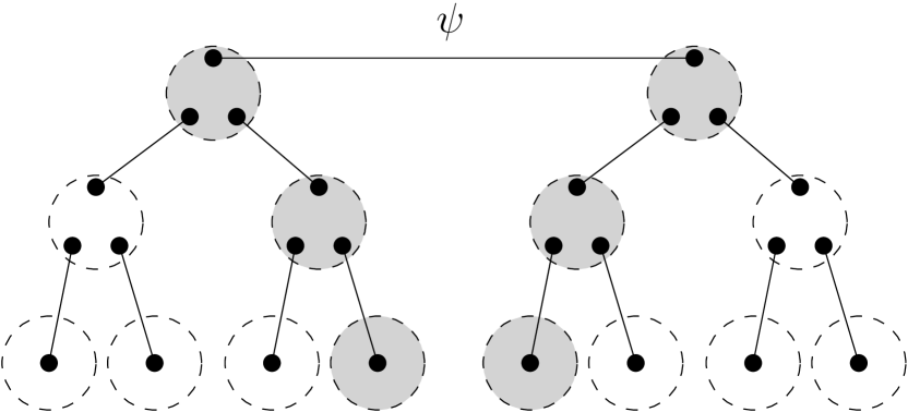
(b)

Figure 4.10: Given a rooted graph $G$ and a multi-qudit state $\psi$ we consider a scenario with an agent for each node of $G$ and qudit of $\psi$. The agents corresponding to the roots have each qudit of $\psi$, and agents given by adjacent nodes have shared entanglement. (a) $\bullet$ denotes a qudit, and each line connecting two dots either the state $\psi$ or a maximally entangled state $\phi$. The set of qudits held by each agent is circled. (b) A path in $G$ for each qudit of $\psi$ defines a sequence of qudits that can be used to implement measurements on $\psi$ by agents that are far away.

In Section 4.2 we showed that measurements on a single-qudit state can be performed at long distances along a line, using only local entanglement and constantly many rounds of local measurements.

We now extend the scenario from a line to a graph and from a single-qudit state to multiple qudits. The purpose of this construction is to show that measurements on a quantum state can be performed in a distributed way, using a simulation with only a constant number of rounds. In Section 4.3.1 we define a simulation for arbitrary measurements using two rounds, in Section 4.3.2 we restrict to Weyl measurements and present a simulation with a single round.

The information specifying the setup is conveniently represented as a rooted graph. We first define rooted graphs and some of their basic properties.

Definition 4.3.1.

A rooted graph $G=(V,E,r)$ is an undirected and connected graph with a distinguished node $r$ called the root.

1. A path is a non-repetitive list of nodes $v_{1}=r,v_{2},\dots,v_{l}$, starting with the root, such that $\{v_{i},v_{i+1}\}\in E$ for all $i=1,\dots,l-1$. Write $\text{Paths}(G)$ for the set of paths in $G$.

2. The neighbourhood of a node $v\in v$ is the set of nodes $N_{G}(v)=\{w\in V\mid\{v,w\}\in E\}$ that are adjacent to $v$.

3. The degree of $G$ is the size of the largest neighbourhood: $\text{deg}(G)=\text{max}_{v\in V}{\left\lvert N_{G}(v)\right\rvert}$.

4. The radius of $G$, denoted by $\text{rad}(G)$, is the least $K\geq 1$ such that every $v\in V$ is reachable by a path of length at most $K$.

Let $\psi$ be a multi-qudit state with qudits labelled by a set $I$ and $G=(V,E,r)$ a rooted graph. We consider a scenario with agents labelled by $I\times V$ (Figure 4.10). The agents share a single instance of the state $\psi$ and a number of maximally entangled two-qudit states $\phi$. Each of the agents $(i,r)\in I\times V$ has qudit $i$ of $\psi$. Additionally, each pair of agents $(i,v),(i,w)\in I\times V$ such that $\{v,w\}\in E$, has one qudit each out of a maximally entangled state. Denote the total state by

$$\lvert\psi,G\rangle :=\lvert\psi\rangle\otimes\bigotimes_{i\in I,\{v,w\}\in E}\lvert\phi\rangle_{(i,v,w),(i,w,v)}$$ (4.23)

The qudit held by agent $(i,v)$ of the maximally entangled state $\lvert\phi\rangle_{(i,v,w),(i,w,v)}$ is labelled by $(i,v,w)$. Agent $(i,r)$ therefore has the following set of qudits

$$\text{Qudits}(i,r) :=\{i\}\cup\{(i,v,w)\mid w\in N_{G}(r)\}$$ (4.24)

where $N_{G}(r)$ is the neighbourhood of the root, and when $v\neq r$ agent $(i,v)$ has qudits

$$\text{Qudits}(i,v) :=\{(i,v,w)\mid w\in N_{G}(v)\}$$ (4.25)

We now consider the following problem. Suppose that we want to perform a measurement on each qudit of $\psi$. How can this be done in such a way that 1) we minimise the probability that any single agent knows the measurement setting, 2) we minimise the number of agents involved in the protocol. The solution is to use the teleportation protocols from the previous section. We first randomly select a path for each qudit $i\in I$. Let $r=v_{1},\dots,v_{j},\dots,v_{l}=v_{i}$ be a path in $G$. We teleport qudit $i$ to agent $(i,v_{i})$ using the sequence of qudits (Figure 4.11)

$$i,(i,v_{1},v_{2}),\dots,(i,v_{j},v_{j-1}),(i,v_{j},v_{j+1}),\dots,(i,v_{l},v_{l-1})$$ (4.26)

Here $(i,v_{j},v_{j+1}),(i,v_{j+1},v_{j})$ are maximally entangled, $i,(i,v_{1},v_{2})\in\text{Qudits}(i,r)$, and $(i,v_{j},v_{j-1}),(i,v_{j},v_{j+1})\in\text{Qudits}(i,v_{j})$ for each $j=2,\dots,l-1$. Hence the protocol uses only local measurements at each agent.

Definition 4.3.2.

Given a rooted graph $G$ let $u_{\text{paths}}\in\mathcal{D}(\text{Paths}(G))$ be any distribution such that for any $v\in V$

$$u_{\text{paths}}(v_{1},\dots,v_{l})>0 \Rightarrow l\leq\text{rad}(G)$$ (4.27)

$$u_{\text{paths}}(v_{1},\dots,v_{l}\text{ such that $v_{l}=v$}) =1/{\left\lvert V\right\rvert}$$ (4.28)

If the paths are chosen independently for each qudit $i$ from the distribution $u_{\text{paths}}$ then the probability that any given player knows the measurement setting is at most $1/{\left\lvert G\right\rvert}$, and the number of agents involved in simulating the measurement on $i$ is at most $\text{rad}(G)$.

4.3.1 Distributing measurements in two rounds

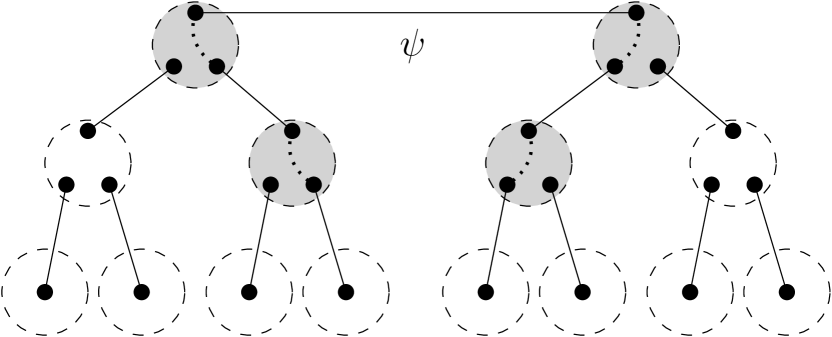
(a)

(b)

Figure 4.11: Simulation protocol. (a) In the first round we perform Bell basis measurements along each path. (b) The first step teleports each qudit up to a Weyl operator phase. In the second round we measure with the corrected measurement.

We now suppose that $S=(I,X,Y)$ is a multipartite scenario, $e$ is a quantum realised empirical model with quantum realisation $(\psi,M)$ in qudit dimension $d$, and $G=(V,E,r)$ is a rooted graph.

We first define a multipartite scenario $T(S,G,d)$. The measurement sites of $T(S,G,d)$ are $I\times V$, and at each measurement site $(i,v)\in I\times V$ the measurement settings and outcomes are as follows. When $v=r$ the measurement settings indicate a measurement setting at measurement site $i$ in the scenario $S$, or one of the neighbors of $r$ in the graph $G$. Otherwise, when $v\neq r$, the measurement settings indicate either one of the measurement settings at measurement site $i$ as well as a neighbour of $v$ in $G$ and one of the Weyl measurement settings $\mathbb{Z}_{d}^{2}$, or two distinct neighbours of $v$ in $G$. For the measurements involving one of the measurements from $S$ the outcomes are the outcomes given by $S$, otherwise the outcomes are $\mathbb{Z}_{d}^{2}$.

Definition 4.3.3.

Let $S=(I,X,Y)$ be a multipartite scenario, $d\geq 2$ a dimension, and $G=(V,E,r)$ a rooted graph. $T(S,G,d)$ is the multipartite scenario with measurement sites $I\times V$ and the following measurement settings and outcomes:

(4.34)

for all $i\in I$ and $v\neq r$.

Next, we define a quantum realised empirical model $e^{\prime}$ for the scenario $T(S,G,d)$. Recall that the quantum realisation $(\psi,M)$ consists of a state $\psi$ with qudits labelled by the measurement sites $I$, and a single-qudit measurement $M_{i,x}$ on qudit $i$, for each measurement $(i,x)$ of the scenario $S$.

To define the empirical model $e^{\prime}$ we interpret the measurement settings of the scenario $T(S,G,d)$ as quantum measurements on the state $\lvert\psi,G\rangle$ in the following way. At each measurement site $(i,r)\in I\times V$ the measurement setting $x$ is the measurement $M_{i,x}$ on qudit $i$, and the measurement setting $w$ is a Bell basis measurement on qudits $i,(i,r,w)$. Otherwise, when $v\neq r$, the measurement setting $(x,w,p)$ is the conjugated measurement $W(p)M_{i,x}W(p)^{\dagger}$ on qudit $(i,v,w)$, and $(w,w^{\prime})$ is a Bell basis measurement on qudits $(i,v,w),(i,v,w^{\prime})$.

Definition 4.3.4.

Let $G=(V,E,r)$ be a rooted graph, $S=(I,X,Y)$ a multipartite scenario, $\psi$ an $I$-qudit state, and $\pi(i,x)$ a single-qudit measurement with outcomes $Y_{i,x}$ for each $i\in I,x\in X_{i}$. $e_{G,\psi,\pi}:S_{G,d}$ is the empirical model realised by the following measurements on $\lvert G,\psi\rangle$.

(4.40)

Using the empirical model $e^{\prime}$ we can simulate the empirical model $e$ in the following way. Suppose that $v$ is a path in $G$. Given any measurement $(i,x)$ on the scenario $S$ we subject the empirical model $e^{\prime}$ to the following measurements. In the case that $v=r$ is the path of length one we perform measurement $x$ on measurement site $(i,r)$. Otherwise, if $v=v_{1},\dots,v_{l}$ then we perform measurement $v_{2}$ on $(i,r)$, and measurement $(v_{j-1},v_{j+1})$ on $(i,v_{j})$ for each $j=2,\dots,l-1$. If the outcomes of these measurements are $p_{1},\dots,p_{l-1}$ then we perform measurement $(v_{l-1},x,\sum_{j=1}^{l-1}q_{j})$ on $(i,v_{l})$. This defines a measurement protocol, which we denote by $C_{v,i,x}$.

$$C_{r,i,x} :=(i,r)\mapsto x$$ (4.41)

and $C_{(v_{1},\dots,v_{l},i,x}=C_{(v_{1},\dots,v_{l},i,x}^{1},C_{(v_{1},\dots,v_{l},i,x}^{2}(s_{1})$, where

$$C_{(v_{1},\dots,v_{l}),i,x}^{1} :=\begin{cases}(i,r)&\mapsto v_{2}\\ (i,v_{j})&\mapsto(v_{j-1},v_{j+1})\end{cases}$$ (4.42)

$$C_{(v_{1},\dots,v_{l}),i,x}^{2}(s_{1}) :=(i,v_{l})\mapsto(v_{l-1},x,\sum_{j=1}^{l-1}s_{1}(i,v_{j}))$$ (4.43)

After performing these measurements we return the outcome of the measurement performed at measurement site $(i,v_{l})$. Write $g_{v,i,x}:\mathcal{E}_{S}(C_{v,i,x})\to Y_{i,x}$ for the function from runs of $C_{v,i,x}$ to outcomes of $(i,x)$.

$$g_{r,i,x} :=s\mapsto s(i,r)$$ (4.44)

$$g_{(v_{1},\dots,v_{l}),i,x} =(s_{1},s_{2})\mapsto s_{2}(i,v_{l})$$ (4.45)

Definition 4.3.5.

Let $G=(V,E,r)$ be a rooted graph, $S=(I,X,Y)$ a multipartite scenario, and $d\geq 2$. $s(S,G,d):T(S,G,d)\to S$ is the simulation

$$\sum_{v\in\text{Paths}(G)^{I}}\big{[}\prod_{i\in I}u_{\text{paths}}(v_{i})\big{]}\cdot t_{v}$$ (4.46)

where for each $v=\{v_{i}\in\text{Paths}(G)\}_{i\in I}$ the deterministic simulation $t_{v}$ is defined by $t_{v}:=(\{C_{v_{i},i,x}\}_{i\in I,x\in X_{i}},\{g_{v_{i},i,x}\}_{i\in I,x\in X_{i}})$.

When one of the deterministic simulations $t_{v}$ is applied to the empirical model $e^{\prime}$ the effect is to perform the two-round teleportation protocol along a choice of path $v_{i}$ for each measurement site $i\in I$. It is therefore clear that $e^{\prime}$ in fact simulates the empirical model $e$.

Lemma 4.3.1.

Let $e_{\psi,M}:S$ be a quantum realised empirical mode, $G=(V,E,r)$ a rooted graph. $s(S,G,d)$ simulates $e_{\psi,M}$ using $e_{G,\psi,M}$ as a resource.

$$s(S,G,d)_{*}(e_{G,\psi,M})=e_{\psi,M}$$ (4.47)

4.3.2 Distributing Weyl measurements in a single round

Consider a multipartite scenario $(I,\mathbb{Z}_{d}^{2},\mathbb{Z}_{d})$, a quantum realised empirical model $e$ along with a quantum realisation $(\psi,W)$ where $W(i,p)$ is the Weyl measurement $W(p)$ on qudit $i$, and $G=(V,E,r)$ a rooted graph.

Figure 4.12: The state $\lvert\psi,G\rangle$ for a two-qudit state $\psi$ and a depth two binary tree. “$\bullet$” denotes a qudit, two qudits connected by a line a maximally entangled state, and each group of qudits is surrounded by a dotted circle.

We first define a multipartite scenario $T(I,G,d)$ with measurement sites $I\times V$. At each measurement site $(i,r)\in I\times V$ the measurement settings are either one of the Weyl measurement settings $\mathbb{Z}_{d}^{2}$ or a neighbour of $r$. Otherwise, when $v\neq r$, the measurement settings at $(i,v)$ are either a distinct pair of neighbours of $v$ or a Weyl measurement setting as well as a neighbour of $v$. The outcomes are either $\mathbb{Z}_{d}^{2}$ or $\mathbb{Z}_{d}$.

Definition 4.3.6.

Let $I$ be a set, $d\geq 2$, and $G=(V,E,r)$ a rooted graph. $T(I,G,d)$ is the multipartite scenario with measurement sites $I\times V$ and the following measurement settings and outcomes:

(4.53)

for all $i\in I$ and $v\neq r$.

We interpret the measurement settings of the scenario $T(I,G,d)$ as quantum measurements on the state $\lvert\psi,G\rangle$. At each measurement site $(i,r)\in I\times V$ measurement setting $p$ is a Weyl measurement $W(p)$ on qudit $i$, and measurement setting $w$ is a Bell basis measurement on qudits $i,(i,r,w)$. Otherwise, when $v\neq r$, measurement setting $(p,w)$ is a Weyl measurement on qudit $(i,v,w)$ and $(w,w^{\prime})$ a Bell basis measurement on qudits $(i,v,w),(i,v,w^{\prime})$.

Definition 4.3.7.

Let $I$ be a set, $d\geq 2$, $\psi$ an $I$-qudit state, and $G=(V,E,r)$ a rooted graph. The empirical model $e_{G,\psi}:S_{G,I,d}$ is the empirical model realised by the state $\lvert G,\psi\rangle$ and measurements:

(4.59)

for all $i\in I$ and $v\neq r$.

We define a simulation from $T(I,G,d)$ to $(I,\mathbb{Z}_{d}^{2},\mathbb{Z}_{2})$ in the following way (Figure 4.12). Given a path $v$ in $G$ an a measurement setting $(i,p)$ for the scenario $(I,\mathbb{Z}_{d}^{2},\mathbb{Z}_{2})$ perform the measurement $p$ on measurement site $(i,r)$ in the case that $v=r$, otherwise if $v=v_{1},\dots,v_{l}$ perform measurement $v_{2}$ on $(i,r)$, $(v_{j-1},v_{j+1})$ on $(i,v_{j})$ where $j=2,\dots,l-1$, and measurement setting $(v_{l-1},p)$ on $(i,v_{l})$. If the outcomes of these measurements are $p_{1},\dots,p_{l-1},q$ then we return the outcome $q-[p,p_{1}+\dots p_{l-1}]$.

Write $f_{v,i,p}$ for the measurement context, and $g_{v,i,p}:\mathcal{E}_{T(I,G,d)}(f_{v,i,p})\to\mathbb{Z}_{d}$ for the outcome map:

$$f_{r,i,p} :=(i,r)\mapsto p$$ (4.60)

$$g_{r,i,p} :=s\mapsto s(i,r)$$ (4.61)

$$f_{(v_{1},\dots,v_{l},i,p} :=\begin{cases}(i,v_{1})&\mapsto v_{2}\\ (i,v_{j})&\mapsto(v_{j-1},v_{j+1})\\ (i,v_{l})&\mapsto(v_{l-1},p)\end{cases}$$ (4.62)

$$g_{v_{1},\dots,v_{l},i,p} :=s\mapsto s(i,v_{l})+[p,\sum_{j=1}^{l-1}s(i,v_{j})]$$ (4.63)

Definition 4.3.8.

Let $I$ be a set, $d\geq 2$, and $G=(V,E,r)$ a rooted graph. $s(I,G,d):T(I,G,d)\to(I,\mathbb{Z}_{d}^{2},\mathbb{Z}_{d})$ is the simulation

$$\sum_{v\in\text{Paths}(G)^{I}}\big{[}\prod_{i\in I}u_{\text{paths}}(v_{i})\big{]}\cdot t_{v}$$ (4.64)

where $t_{v}$ is the deterministic simulation $(\{f(v_{i})_{i,p}\}_{i\in I,p\in\mathbb{Z}_{d}^{2}},\{g(v_{i})_{i,p}\}_{i\in I,p\in\mathbb{Z}_{d}^{2}})$.

When the simulation is applied to the empirical model $e$ the effect is to perform the single-round teleportation protocol on a line. It is therefore clear that the pushforward of $e_{G,\psi,M}$ is $e$.

Lemma 4.3.2.

Let $e_{\psi}:(I,\{\mathbb{Z}_{d}^{2}\},\{\mathbb{Z}_{d}\})$ be a Pauli measurement model and $G$ a rooted graph. $s_{G}:S_{G,I,d}\to(I,\mathbb{Z}_{d}^{2},\mathbb{Z}_{d})$ simulates $e_{\psi}$ using $e_{\psi,G}$ as a resource.

$$(s_{G})_{*}(e_{\psi,G})=e_{\psi}$$ (4.65)

4.4 Distributing non-local games on graphs

In Section 4.3 we showed that measurements on a multi-qudit state can be simulated in a distributed way, using a graph as a template. We now use this construction to define distributed versions of non-local games and show that they are solved by quantum circuits of low depth and fan-in. We present two versions of this. In Section 4.4.1 we use the two-round teleportation protocol, and we work with general non-local games. In Section 4.4.2 we use the single-round protocol and we restrict attention to non-local games using Weyl measurements.

4.4.1 Two-round distributed non-local games

Let $S=(I,X,Y)$ be a multipartite scenario, $(e,\Phi)$ a non-local game along with a quantum realisation $(\psi,M)$ of $e$ in qudit dimension $d\geq 2$, and $G=(V,E,r)$ a rooted graph.

In Section 4.3.1 we defined a measurement scenario $T(S,G,d)$, a quantum realised empirical model $e^{\prime}$, and a simulation $s(S,G,d):T(S,G,d)\to S$ such that ${s(S,G,d)}_{*}(e^{\prime})=e$. We now consider the pullback of the cooperative game $\Phi$ across the simulation $s(S,G,d)$. Because $e^{\prime}$ simulates $e$ we have that the success probability of $e^{\prime}$ on the pullback problem is equal to the success probability of $e$. $e^{\prime}$ therefore violates the classical bound for the non-local game $(e,\Phi)$.

$$p_{S}(e^{\prime},{s(S,G,d)}^{*}(\Phi))=p_{S}(e,\Phi)>\gamma$$ (4.66)

where $\gamma$ is the classical bound.

We can implement $e^{\prime}$ as a two-round quantum circuit strategy (Figure 4.13). We first have to prepare $\lvert\psi,G\rangle$. This can be done with a single unitary gate of fan-in ${\left\lvert I\right\rvert}$ and a number of unitary two-qudit gates. We then have to implement measurements. The measurements corresponding to each measurement site $(i,v)$ act on $\text{Qudits}(i,v)$. The fan-in of these gates, therefore, depends only on the degree of $G$.

(a)

$$U_{\psi,G} =U_{\psi}\otimes\bigotimes_{i\in I,\{v,w\}\in E}U_{(i,v,w),(i,w,v)}$$

$$U_{\psi}\lvert 0\dots 0\rangle =\lvert\psi\rangle$$

$$U_{(i,v,w),(i,w,v)}\lvert 00\rangle =\lvert\phi\rangle$$

(b)

Measurement site	Input value	Measurement setting
$(i,r)$	$w\in N_{G}(r)$	Bell basis on qudits $i,(i,r,w)$
	$x\in X_{i}$	$M_{i,x}$ on qudit $i$
	$\bullet$	Identity
$(i,v)$	$w,w^{\prime}\in N_{G}(v).\ w\neq w^{\prime}$	Bell basis on qudits $(i,v,w),(i,v,w^{\prime})$
	$(x,w,p)\in X_{i}\times N_{G}(v)\times\mathbb{Z}_{d}^{2}$	$W(p)M_{i,x}W(-p)$ on qudit $(i,v,w)$
	$\bullet$	Identity

(c)

Figure 4.13: The two-round quantum circuit strategy $Q_{G,\psi,M}$ uses a multi-qudit register initially set to the computational basis state. The state $\lvert\psi,G\rangle$ is prepared by a single ${\left\lvert I\right\rvert}$-qudit gate $U_{\psi}$ and a two-qudit gate $U_{(i,v,w),(i,w,v)}$ for each $i\in I,\{v,w\}\in E$. The first round of inputs $x_{i,v}$ is used to control a non-destructive measurement gate $M_{i,v}$ with measurement settings given by (b), and the second round of inputs $x_{(i,v)}^{\prime}$ controls a destructive measurement gate $M_{i,v}^{\prime}$ also with measurement settings from (b).

Lemma 4.4.1.

Let $S=(I,X,Y)$ be a multipartite scenario and $(e,\Phi)$ a non-local game with classical bound $\gamma$. Suppose that $e$ has a quantum realisation in qudit dimension $d\geq 2$. There exists a two-round cooperative game $\Phi^{\prime}$ with classical bound $\gamma$ and quantum circuit strategy $Q$ such that

1. The success probability of $Q$ exceeds $\gamma$: $p_{S}(Q,\Phi^{\prime})>\gamma$.

2. The depth and maximal fan-in of $Q$ depends only on the size of $I$ and the degree of $G$.

(a)

(b)

Figure 4.14: (a) A generic two-player Weyl measurement game. Alice and Bob share a two-qudit state $\psi$. Verifier randomly selects $q_{1},q_{2}\in\mathbb{Z}_{2}^{2}$ and an accepting condition $A\subset\mathbb{Z}_{d}^{2}$ according to a probability distribution $d(q_{1},q_{2},A)$. Alice and Bob measure the Weyl measurements $W(p_{1}),W(p_{2})$ respectively. Their success probability is the likelihood that $(q_{1},q_{2})\in A$. (b) Graph version of the game (a) played on a tree. randomly selects paths $(r,v_{11},\dots,v_{1k_{1}}),(r,v_{21},\dots,v_{2k_{2}})$ according to a path distribution $d_{\text{paths}}$ and an instance $(p_{1},p_{2},A)$ of (a) with probability $d(p_{1},p_{2},A)$. Verifier sends players $(1,r),(1,v_{11}),\dots,(1,v_{1k_{1}})$ They win if $(q_{1}^{\prime}+[p_{1},p_{1}^{\prime}],q_{2}^{\prime}+[p_{2},p_{2}^{\prime}])\in A$, where $p_{i}^{\prime}=p_{i1}^{\prime}+\dots+p_{i2}^{\prime}$.

4.4.2 Single-round distributed Weyl-measurement games

Let $(e,\Phi)$ be a non-local game for a multipartite scenario on the form $(I,\mathbb{Z}_{d}^{2},\mathbb{Z}_{d})$, such that $e$ has a quantum realisation on an $I$-qudit state $\psi$, where the measurement $(i,p)$ is the Weyl measurement $W(p)$ on qudit $i$. Let $G=(V,E,r)$ be a rooted graph.

In Section 4.3.2 we defined a quantum realised empirical model $e^{\prime}$ and a single-round simulation $s(I,G,d)$ such that ${s(I,G,d)}_{*}(e^{\prime})=e$. Taking the pullback $s(I,G,d)^{*}(\Phi)$ we then have

$$p_{S}(e^{\prime},s(I,G,d)^{*}(\Phi))>\gamma$$ (4.67)

where $\gamma$ is the classical bound of $(e,\Phi$. We can implement $e^{\prime}$ as the quantum circuit in Figure (4.15).

Lemma 4.4.2.

Let $(e,\Phi)$ be a Weyl measurement game with classical bound $\gamma$ and $G$ a rooted graph. Consider the pullback of $\Phi$ across the single-round simulation. This game has a quantum circuit strategy $Q$ such that that

1. The success probability of $Q$ at the pullback of $\Phi$ is the success probability of $e$ at $\Phi$, which exceeds $\gamma$: $p_{S}(Q,s(I,G,d)^{*}(\Phi))>\gamma$.

2. The depth and maximal fan-in of $Q$ is only dependent on the size of $I$ and the degree of $G$.

We can describe the pullback game more directly as follows. Recall $\Phi$ is defined as a convex combination $\sum_{U,A}\Phi_{U,A}\cdot(U,A)$ where $U$ is a joint measurement for the scenario $(I,\mathbb{Z}_{d}^{2},\mathbb{Z}_{d})$ and $A\subset\mathcal{E}_{(I,\mathbb{Z}_{d}^{2},\mathbb{Z}_{d})}(U)$ is an accepting condition.

In the pullback game Verifier randomly selects $U,A$ with probability $\Phi_{U,A}$. For each joint input $(i,p_{i})\in U$ Verifier then selects a path $v_{i}=(v_{i1},\dots,v_{il_{i}})$ in $G$ with probability $u_{\text{paths}}(v_{i})$. If $v_{i}$ is the trivial path then Verifier gives input $p_{i}$ to $(i,r)$, otherwise if $l>1$, Verifier gives input $v_{i2}$ to $(i,r)$, input $(v_{i(j-1)},v_{i(j+1)})$ to $(i,v_{j})$, and finally input $(v_{i(l_{i}-1)},p_{i})$ to and $(i,v_{l_{i}})$. The total joint input is then

$$U_{v}:=\begin{cases}(i,r)\mapsto p_{i},&\text{if $(i,p_{i})\in U$ and $v_{i}=r$}\\ (i,r)\mapsto v_{2},&\text{if $(i,p_{i})\in U$ and $l_{i}>1$}\\ (i,v_{ij}\mapsto(v_{i(j-1)},v_{i(j+1)}),&\text{if $(i,p_{i})\in U$ and $j=2,\dots,l_{i}-1$}\\ (i,v_{il_{i}})\mapsto(v_{i(l_{i}-1)},p_{i}),&\text{if $(i,p_{i})\in U$ and $l_{i}>2$}\end{cases}$$ (4.68)

The players then respond with a joint output $s\in\mathcal{E}_{S_{G,I,d}}(U_{v,p})$. The output is accepted if

$$A_{v,U}(s):\iff\big{(}(i,p_{i})\mapsto s(i,v_{il_{i}})+[p_{i},\sum_{j=1}^{l_{i}-1}s(i,v_{ij})]\big{)}_{(i,p_{i})\in U}\in A$$ (4.69)

As a convex combination the pullback is then the game

$$\sum_{v,U,A}\big{[}\prod_{i\in I}u_{\text{paths}}(v_{i})\big{]}\Phi_{U,A}\cdot(U_{v},A_{v,U})$$ (4.70)

(a)

$$U_{\psi,G} =U_{\psi}\otimes\bigotimes_{i\in I,\{v,w\}\in E}U_{(i,v,w),(i,w,v)}$$

$$U_{\psi}\lvert 0\dots 0\rangle =\lvert\psi\rangle$$

$$U_{(i,v,w),(i,w,v)}\lvert 00\rangle =\lvert\phi\rangle$$

(b)

Input wire	Value	Measurement setting
$(i,r)$	$p\in\mathbb{Z}_{d}^{2}$	$W(p)$ on qudit $i$
	$w\in N_{G}(r)$	Bell basis on qudits $i$ $(i,r,w)$
	$\bullet$	Identity measurement
$(i,v)$	$(w,p)\in N_{G}(v)\mathbb{Z}_{d}^{2}$	$W(p)$ on qudit $(i,v,w)$
	$(w,w^{\prime})\in N_{G}(v)^{2}.\ w\neq w^{\prime}$	Bell basis on qudits $(i,v,w)$ $(i,v,w^{\prime})$
	$\bullet$	Identity measurement

(c)

Figure 4.15: (a) Circuit strategy $Q_{\psi,G}$, where $\psi$ is an $n$-qudit state and $G=(V,E,r)$ is a rooted graph. to entangle each qudit of $\psi$ with a qudit that is far away in the circuit and measures this qudit in the Weyl basis. (b) The effect of the Bell basis measurements is to teleport $\psi$ up to a random phase.

4.5 Separating quantum and classical circuits of low depth and fan-in

In Section 4.3 we defined two simulations $s(S,G,d)$ and $s(I,G,d)$ with respectively one and two rounds, that perform measurements on a quantum state in a distributed way. The simulations where then used in Section 4.4 to define distributed versions of non-local games, such that the quantum strategies can be recast as circuits of small depth and fan-in. The purpose of this section is to bound the success probability of classical circuits on these problems. Recall the resource inequality

$$p_{S}(e^{\prime},\Phi)\leq\gamma+\text{CF}(e^{\prime})$$ (4.71)

relating the success probability of an arbitrary empirical model $e^{\prime}$ to the classical bound $\gamma$ for a non-local game and its contextual fraction $\text{CF}(e^{\prime})$. We observe that the derivation of this bound does not rely on the no-disturbance condition. In Section 4.1 we explained that circuit strategies give rise to empirical models that don’t satisfy the no-disturbance condition, we called these objects “behaviours”, and explained that constructions like simulations and the contextual fraction can be generalised. Because the bound $\gamma+\text{CF}(e^{\prime})$ does not rely on no-disturbance we have a bound

$$p_{S}(B,\Phi)\leq\gamma+\text{CF}(B)$$ (4.72)

for any behaviour $B$.

We want to bound the contextual fraction of a classical circuit $C$ on the pullback $s^{*}(\Phi)$ of a game $\Phi$ across some simulation $s$. To do this we bound the contextual fraction of the pushforward $s_{*}(\tilde{C})$ and rely on the inequality 4.72.

Although we use a different terminology this is precisely what Bravyi, Gosset, and König did. We will work at a general level, first stating the result as a general property of simulations, and then restrict to the two simulations.

The idea is to consider a general simulation $s:S\to T$. Recall that $s$ is defined as a probability distribution over deterministic simulations $t:S\to T$. In Section 4.5.1 we consider the case of a deterministic simulation. We derive a combinatorial condition involving the lightcones of the circuit $C$ that ensures that the pushforward $t_{*}(\tilde{C})$ is non-contextual. In Section 4.5.2 we first present a lemma due to BGK, and we restate this as a bound on the probability that this condition holds, when $t$ is selected randomly from a simulation $s$. We finally apply this to the simulations $s(G,I,d)$ and $s(S,G,d)$.

4.5.1 Lightcones of simulations

The simulations $s(S,G,d)$ and $s(I,G,d)$ are defined as probability distributions over deterministic simulations $t_{v}$ corresponding to each choice of paths $v\in\text{Paths}(G)^{I}$. Consider these simulations for a fixed choice of paths $v$. The measurements performed in these simulations are independent of the input for all but a small number of measurement sites, and the outcome we return only depends on the outcomes of the measurements on a small number of measurement sites. In the two-round case, given a measurement $(i,x)$ for the scenario $S$ we first perform a measurement $C_{v_{i},i,x}^{1}$ that is independent of $x$ and in the second round we perform a measurement $C_{v_{i},i,x}$ that is only defined on $(i,v_{il_{i}})$. The final outcome only depends on the outcome at $(i,v_{il_{i}})$. In the single-round case, we perform a single measurement where only the setting at $(i,v_{il_{i}})$ depends on $x$. And the outcome returned depends only on the subset of measurement sites $\{(i,v_{ij})\}$.

For any deterministic simulation $t:S\to T$ we can identify the unique minimal subset of measurement sites such that the measurement setting in round $k$ depends on the input, and the outcome uses the measurement outcome. For each round $k\leq n$ and $j\in J$ we define the input and output dependencies of the simulation as follows.

Definition 4.5.1.

Let $S=(I,X,Y),T=(J,Z,W)$ be two multipartite scenarios and $t=(\{C_{j,z}\}_{j\in J,z\in Z_{j}},\{g_{j,z}\}_{j\in J,z\in Z_{j}}):S\to T$ an $n$-round deterministic simulation, where $C_{j,z}$ is the measurement protocol

$$C_{i,z}=C_{i,z}^{1},\dots,C_{i,z}^{k}(s_{1},\dots,s_{k-1}),\dots,C_{i,z}^{n}(s_{1},\dots,s_{n-1})$$ (4.73)

and $g_{j,z}:\mathcal{E}_{S}(C_{j,z})\to W_{j,z}$. For any measurement site $j\in J$ and round $k=1,\dots,n$ let $\text{In}_{k}(t)(j),\text{Out}_{k}(t)(j)\subset I$ as follows

• $\text{In}_{k}(t)(j)$ is the least $I^{\prime}\subset I$ such that for each $z\in Z_{j}$ and run $(s_{1},\dots,s_{n})\in\mathcal{E}_{S}(C_{j,z})$ the joint measurement $C_{j,z}^{k}(s_{1},\dots,s_{k-1})$ can be written as a union

  $$C_{j,z}^{k}(s_{1},\dots,s_{k-1})=U(s_{1},\dots,s_{k-1})\cup U_{z}(s_{1},\dots,s_{k-1})$$ (4.74)

  where $U(s_{1},\dots,s_{k-1})$ is independent of $z$ and $U_{z}(s_{1},\dots,s_{k-1})$ is a joint measurement for the measurement sites $I^{\prime}$.

• $\text{Out}_{k}(t)(j)\subset I$ is the least $I^{\prime}\subset I$ such that for each run $(s_{1},\dots,s_{n})\in\mathcal{E}_{S}(C_{j,z})$ the outcome $g_{j,z}(s_{1},\dots,s_{n})\in W_{j,z}$ is independent of the value of $s_{k}$ on measurement sites $I\setminus I^{\prime}$:

  $$g_{j,z}(s_{1},\dots,s_{n})=g_{j}(s_{1},\dots,s_{k}\rvert_{I^{\prime}},\dots,s_{n})(x)$$ (4.75)

  where $g_{j}$ is some function.

For example, for the two-round simulation $t:=t(S,G,d,v)$ we have

$$\text{In}_{1}(t)(i) =\emptyset$$ (4.76)

$$\text{In}_{2}(t)(i) =\{(i,v_{il_{i}})\}$$ (4.77)

$$\text{Out}_{2}(t)(i) =\{(i,v_{il_{i}})\}$$ (4.78)

and for the single-round simulation $t:=t(I,G,d,v)$

$$\text{In}_{1}(t)(i) =\{(i,v_{il_{i}})\}$$ (4.79)

$$\text{Out}_{1}(t)(i) =\{(i,v_{ij})\}_{j=1}^{l_{i}}$$ (4.80)

If $t:S\to T$ is an $n$-round simulation such that $\text{In}_{k}(t)(j)$ is empty for all $k<n$ and $C$ is a classical strategy such that $t_{*}(\tilde{C})$ is contextual. Then there must be some $j\neq j^{\prime}$ and $i\in\text{In}_{n}(t)(j),i^{\prime}\in\text{Out}_{n}(t)(j^{\prime})$ such that there is path through $C$ from $\text{in}_{in}$ to $\text{out}_{i^{\prime}n}$. Let the relation $\text{In}_{n}(t);\text{LC}_{C}^{\leftarrow};\text{Out}_{n}(t)\subset J\times J$ be defined by

$$\exists i,i^{\prime}\in I:\ i\in\text{In}_{n}(t)(j)\land\text{in}_{ni}\in\text{LC}_{C}^{\leftarrow}(\text{out}_{ni^{\prime}})\land i^{\prime}\in\text{Out}_{n}(j^{\prime})$$ (4.81)

for all $(j,j^{\prime})\in J\times J$ (Figure 4.16). In other words, if $\text{In}_{n}(t);\text{LC}_{C}^{\leftarrow};\text{Out}_{n}(t)\subset\text{id}_{J}$, where $\text{id}_{J}\subset J\times J$ is the identity relation, then $t_{*}(\tilde{C})$ is non-contextual.

(a) $\text{In}_{1}(t)$

(b) $\text{LC}_{C}^{\leftarrow}$

(c) $\text{Out}_{1}(t)$

(d) $\text{In}_{1}(t);\text{LC}_{C}^{\leftarrow};\text{Out}_{1}(t)$

Figure 4.16: Consider a simulation $t$ from a scenario with measurement sites $\{1,2\}$ to a scenario with measurement sites $\{A,B,C,D\}$ with the input dependencies in (a) and the output dependencies in (c) and a classical circuit $C$ with lightcones in (b).

Lemma 4.5.1.

Let $S$ and $T=(J,Z,W)$ be two multipartite scenarios, $t:S\to T$ an $n$-round deterministic simulation, and $C$ an $n$-round classical circuit strategy for $S$. If for all $k<n$ and $j\in J$ we have $\text{In}_{k}(t)(j)=\emptyset$, and $\text{In}_{n}(t);\text{LC}_{C}^{\leftarrow};\text{Out}_{n}(t)\subset\text{id}_{J}$ then $t_{*}(\tilde{C})$ is non-contextual.

Proof.

Let $t:S\to T$ be an $n$-round deterministic simulation and $C$ an $n$-round classical circuit strategy. By definition $t_{*}(\tilde{C})$ is defined for any context $U$ of $T$ by

$$t_{*}(\tilde{C})(U)=\sum_{(s_{1},\dots,s_{n})\in\mathcal{E}_{S}(f(U))}\tilde{C}(f(U))(s_{1},\dots,s_{n})\cdot g_{U}(s_{1},\dots,s_{n})$$ (4.82)

where $f(U)\in\text{MP}_{n}(S)$ and $g_{U}:\mathcal{E}_{S}(f(U))\to\mathcal{E}_{T}(U)$. By assumption the first $n-1$ measurements are independent of $U$, so that $f(U)$ is of the form:

$$f(U)=V_{1},V_{2}(s_{1}),\dots,V_{n-1}(s_{1},\dots,s_{n-2}),V_{n}(U)(s_{1},\dots,s_{n-1})$$ (4.83)

Because $C$ is a classical circuit we can write the probability distribution $\tilde{C}(F(U))$ as a convex combination of hidden variables $\lambda$, such that

$$\tilde{C}(f(U))=\sum_{\lambda}p_{\lambda}\cdot(\lambda_{1},\dots,\lambda_{n-1},\lambda_{n}(V_{n}(U)(\lambda_{1},\dots,\lambda_{n-1})))$$ (4.84)

and the value of $\lambda_{n}(U)(\lambda_{1},\dots,\lambda_{n-1})$ at any measurement site $i\in I$ depends only on the measurement setting of $V_{n}(U)$ on the subset of measurement sites

$$\overleftarrow{i}=\{i^{\prime}\in I\mid\text{in}_{i^{\prime}}\in\text{LC}_{C}^{\leftarrow}(\text{out}_{i})\}$$ (4.85)

Plugging the hidden variable expression for $\tilde{C}(f(U))$ into the first equation we get a hidden variable expression for the pushforward $t_{*}(\tilde{C})(U)$

$$t_{*}(\tilde{C})(U)=\sum_{\lambda}p_{\lambda}\cdot g_{U}(\lambda_{1},\dots,\lambda_{n-1},\lambda_{n}(V_{n}(U)(\lambda_{1},\dots,\lambda_{n-1})))$$ (4.86)

To see that $t_{*}(\tilde{C})$ it is sufficient to show that the value of

$$g_{U}(\lambda_{1},\dots,\lambda_{n-1},\lambda_{n}(V_{n}(U)(\lambda_{1},\dots,\lambda_{n-1})))$$ (4.87)

on a measurement $(j,z)$ is independent of $U$.

Suppose therefore that $(j,z)$ is any measurement for $T$ and for any $U$ consider the outcome assigned to $(j,z)$. That is, the value

$$g_{U}(\lambda_{1},\dots,\lambda_{n-1},\lambda_{n}(V_{n}(U)(\lambda_{1},\dots,\lambda_{n-1})))(j,z)$$ (4.88)

First we have that the outcome of $(j,z)$ only depends on the value of $\lambda_{n}(V_{n}(U)(\lambda_{1},\dots,\lambda_{n-1})))$ on the subset of measurement sites $\text{Out}_{n}(t)(j)\subset I$. Furthermore, the value of $\lambda_{n}(V_{n}(U)(\lambda_{1},\dots,\lambda_{n-1})))$ on measurement sites $\text{Out}_{n}(t)(j)$ depends only on the value of $V_{n}(U)(\lambda_{1},\dots,\lambda_{n-1}))$ on

$$\overleftarrow{\text{Out}_{n}(t)(j)}:=\bigcup_{i\in\text{Out}_{n}(t)(j)}\overleftarrow{i}$$ (4.89)

Hence the outcome of $(j,z)$ depends only on the value of $V_{n}(U)(\lambda_{1},\dots,\lambda_{n-1})$ on each $i^{\prime}$ such that there exists an $i$ such that $\text{in}_{i^{\prime}n}\in\text{LC}_{C}^{\leftarrow}(\text{out}_{in}$ and $i\in\text{Out}_{n}(t)(j)$. Finally, we have that the value of $V_{n}(U)(\lambda_{1},\dots,\lambda_{n-1})$ on $i$ only depends on the value of $U$ on $j$ such that $i\in\text{In}_{n}(t)(j)$. Therefore, if the condition holds then it is non-contextual. ∎

4.5.2 Classical bound

Suppose that $s:S\to T$ is a probabilistic simulation from a multipartite scenario $S$ to another multipartite scenario $T$ and $C$ a classical strategy for $S$. Suppose that we randomly select a deterministic simulation $t:S\to T$ with probability given by $s$. Lemma 4.5.1 gives a condition ensuring that the pushforward $t_{*}(\tilde{C})$ is non-contextual, involving the relation $\text{In}_{n}(t);\text{LC}_{C}^{\leftarrow};\text{Out}_{n}(t)$. We now consider the probability that this condition is satisfied when $t$ is chosen randomly from the simulation $s$.

The following lemma from BGK shows that $C$ has low depth and fan-in, $\text{In}_{n}(t)(j)$ is small, and $\text{Out}_{n}(t)(j)$ is distributed in a uniform way, then the probability that the condition holds is high.

Lemma 4.5.2.

(BGK) Let $C$ be a circuit with inputs $\{\text{in}_{i}\}_{i\in I}$ and outputs $\{\text{out}_{i}\}_{i\in I}$ of depth $D$ and fan-in at most $K$. Suppose that we randomly select a family of sets $\{I_{\text{in}}(j),I_{\text{out}}(j)\subset I\}_{j\in J}$ and consider the relation $I_{\text{in}};\text{LC}_{C}^{\leftarrow};I_{\text{out}}\subset J\times J$ given by

$$\exists i,i^{\prime}\in I.\ i\in I_{\text{in}}(j)\land\text{in}_{i}\in\text{LC}_{C}^{\leftarrow}(\text{out}_{i^{\prime}})\land i^{\prime}\in I_{\text{out}}(j^{\prime})$$ (4.90)

for all $(j,j^{\prime})\in J\times J$. Suppose that the following conditions hold:

1. The size of $I_{\text{out}}(j)$ is at most $A$, for all $j\in J$.

2. For all $j\in J$ and $i\in I$. If we randomly select $\{I_{\text{in}}(j),I_{\text{out}}(j)\}_{j\in J}$ from the marginal distribution fixing $I_{\text{out}}(j)$, then for each $j^{\prime}\in J$, such that $j\neq j^{\prime}$, the probability that $i\in I_{\text{in}}(j)$ is at most $\epsilon$:

   $$\text{Prob}(i\in I_{\text{in}}(j)\mid I_{\text{out}}(j^{\prime}))\leq\epsilon$$ (4.91)

The probability that the condition $I_{\text{in}};\text{LC}_{C}^{\leftarrow};I_{\text{out}}\subset\text{id}_{J}$ fails is at most $K^{D}{\left\lvert J\right\rvert}^{2}A\epsilon$.

Proof.

For some $j\neq j^{\prime}\in J$ suppose that $I_{\text{out}}(j^{\prime})$ is fixed and that $I_{\text{in}}(j)$ is chosen randomly.

$$\text{Prob}(\text{LC}_{C}(I_{\text{in}}(j),I_{\text{out}}(j^{\prime}))) \leq\sum_{i\in I_{\text{out}}(j^{\prime})}\text{Prob}(\text{LC}_{C}(I_{\text{in}}(j),i)$$ (4.92)

$$\leq\sum_{i\in\text{LC}_{C}^{\leftarrow}(I_{\text{out}}(j^{\prime}))}\text{Prob}(i\in I_{\text{in}}(j))$$ (4.93)

$$\leq\sum_{i\in\text{LC}_{C}^{\leftarrow}(I_{\text{out}}(j^{\prime}))}\epsilon$$ (4.94)

$$\leq K^{D}A\epsilon$$ (4.95)

If $\{I_{\text{in}}(j),I_{\text{out}}(j)\subset I\}_{j\in J}$ is chosen randomly we therefore have by the union bound that

$$\text{Prob}(\exists j\neq j^{\prime}\in J.\ \text{LC}_{C}(I_{\text{in}}(j),I_{\text{out}}(j^{\prime}))) \leq\sum_{j\neq j^{\prime}\in J}\text{Prob}(\text{LC}_{C}(I_{\text{in}}(j),I_{\text{out}}(j^{\prime})))$$ (4.96)

$$\leq\frac{{\left\lvert J\right\rvert}({\left\lvert J\right\rvert}-1)}{2}K^{D}A\epsilon$$ (4.97)

$$\leq{\left\lvert J\right\rvert}^{2}K^{D}A\epsilon$$ (4.98)

∎

We next restate this as a bound on the contextual fraction.

Lemma 4.5.3.

Let $S$ and $T$ be two multipartite scenarios, $s:S\to T$ an $n$-round simulation, and $C$ a classical $n$-round circuit strategy of depth $D$ and maximal fan-in $K$. Suppose that the following conditions hold when a deterministic simulation $t$ is chosen randomly with probability $s(t)$:

• For each $k<n$ and $j\in J$ we have $\text{In}_{k}(t)(j)=\emptyset$.

• For each $j\in J$ we have ${\left\lvert\text{In}_{n}(t)(j)\right\rvert}\leq A$.

• For all $j,j^{\prime}\in J$ and $i\in I$ such that $j\neq j^{\prime}$:

  $$s(i\in\text{In}_{n}(t)(j)\mid\text{Out}_{n}(t)(j^{\prime}))\leq\epsilon$$ (4.99)

The contextual fraction of the pushforward $s_{*}(\tilde{C})$ is at most ${\left\lvert J\right\rvert}^{2}K^{D}A\epsilon$

$$\text{CF}(s_{*}(\tilde{C}))\leq{\left\lvert J\right\rvert}^{2}K^{D}A\epsilon$$ (4.100)

Proof.

The pushforward $s_{*}(\tilde{C})$ is defined for each context $U$ of $T$ as the convex combination

$$s_{*}(\tilde{C})(U)=\sum_{t}s(t)\cdot t_{*}(\tilde{C})(U)$$ (4.101)

The non-contextual fraction of $s_{*}(\tilde{C})$ (Definition 2.6.1) is the greatest weight assigned to the non-contextual part of any convex decomposition of $s_{*}(\tilde{C})$ into a non-contextual model and another empirical model. The non-contextual fraction of $s_{*}(\tilde{C})$ is therefore bounded from below by the probability that $t_{*}(\tilde{C})$ is non-contextual when $t$ is chosen randomly according to $s$.

$$s(t_{*}(\tilde{C})\text{ is non-contextual})\leq\text{NCF}(s_{*}(\tilde{C}))$$ (4.102)

Or equivalently

$$\text{CF}(s_{*}(\tilde{C}))\leq s(t_{*}(\tilde{C})\text{ is contextual})$$ (4.103)

By Lemma 4.5.1 if $t_{*}(\tilde{C})$ is contextual then $\text{In}_{n}(t);\text{LC}_{C}^{\leftarrow};\text{Out}_{n}(t)\not\subset\text{id}_{I}$.

$$s(t_{*}(e)\text{ is contextual})\leq s(\text{In}_{n}(t);\text{LC}_{C}^{\leftarrow};\text{Out}_{n}(t)\not\subset\text{id}_{I})$$ (4.104)

By Lemma 4.5.2 the probability of $\text{In}_{n}(t);\text{LC}_{C}^{\leftarrow};\text{Out}_{n}(t)\not\subset\text{id}_{J}$ is at most ${\left\lvert J\right\rvert}^{2}K^{D}A\epsilon$, as required. ∎

We now consider the two simulations $s(S,G,d),s(I,G,d)$ from Section 4.3.

Lemma 4.5.4.

Let $G$ be a rooted graph, $d\geq 2$ a dimension, $I$ a finite set, and $S=(I,X,Y)$ a multipartite scenario.

1. Let $C$ a two-round classical circuit strategy for the scenario $T(S,G,d)$ of depth $D$ and maximal fan-in $K$.

   $$\text{CF}(s(S,G,d)_{*}(\tilde{C}))\leq{\left\lvert I\right\rvert}^{2}K^{D}{\left\lvert G\right\rvert}^{-1}$$ (4.105)

2. Let $C$ be a single-round classical circuit strategy for the scenario $T(I,G,d)$ of depth $D$ and maximal fan-in $K$.

   $$\text{CF}(s(I,G,d)_{*}(\tilde{C}))\leq{\left\lvert I\right\rvert}^{2}K^{D}{\left\lvert G\right\rvert}^{-1}\text{rad}(G)$$ (4.106)

Proof.

In each case the simulation is defined as a convex combination

$$\sum_{v\in\text{Paths}(G)^{I}}\big{[}\prod_{i\in I}u_{\text{paths}}(v_{i})\big{]}\cdot t_{v}$$ (4.107)

where $t_{v}$ is a simulation with either

$$\text{In}_{1}(t)(i) =\emptyset$$ (4.108)

$$\text{In}_{2}(t)(i) =\{(i,v_{il_{i}})\}$$ (4.109)

$$\text{Out}_{2}(t)(i) =\{(i,v_{il_{i}})\}$$ (4.110)

in the two-round case, or

$$\text{In}_{1}(t)(i) =\{(i,v_{il_{i}})\}$$ (4.111)

$$\text{Out}_{1}(t)(i) =\{(i,v_{ij})\}_{j=1}^{l_{i}}$$ (4.112)

in the single-round case.

In either case condition 1. of Lemma 4.5.3 is satisfied. For the second condition we have $A=1$ in the first case and $A\leq\text{rad}(G)$ in the second case.

Note that choice of paths are independent for different $i,i^{\prime}\in I$. For the third condition we therefore have bound $\epsilon=1/{\left\lvert G\right\rvert}$. ∎

4.5.3 Randomised restrictions

A common technique in complexity theory is to look at randomised restrictions of circuits. In this section we explain why this is not sufficient to prove a separation between shallow quantum and classical circuits.

Definition 4.5.2.

Let $S=(I,X,Y)$ be a multipartite scenario and $B$ a single-round behaviour. A restriction is a pair $(U,I^{\prime})$ where $I^{\prime}\subset I$ is a subset of measurement sites and $U$ is a joint measurement for the remaining measurement sites $I\setminus I^{\prime}$. Write $S\rvert_{I^{\prime}}$ for the multipartite scenario $(I^{\prime},(X_{i})_{i\in I},(Y_{i,x})_{i\in I^{\prime},x\in X_{i}})$ and $e\rvert_{U,I^{\prime}}:S\rvert_{I^{\prime}}$ for the behaviour given by fixing the measurement setting at measurement sites $I\setminus I^{\prime}$ according to $x$.

Let $C$ be a classical circuit strategy of depth $D$ and maximal fan-in $K$. We consider the probability that $\tilde{C}\rvert_{U,I^{\prime}}$ is contextual when $(U,I^{\prime})$ is selected randomly. Classically we require communication to produce contextuality: If $\tilde{C}$ is contextual then there must be some some $i\neq i^{\prime}\in I$ such that input wire $i$ communicates to output wire $i^{\prime}$ through $C$, i.e. $\text{in}_{i}\in\text{LC}_{C}^{\leftarrow}(\text{out}_{i^{\prime}})$. Hence if the restriction $\tilde{C}\rvert_{U,I^{\prime}}$ is contextual then there are $i\neq i^{\prime}\in I^{\prime}$ such that $\text{in}_{i}\in\text{LC}_{C}^{\leftarrow}(\text{out}_{i^{\prime}})$. Because $I^{\prime}$ is small and uniformly distributed it can be shown that the probability that this occurs is at most $\epsilon K^{D}$ for some small $\epsilon$. $\tilde{C}\rvert_{U,I^{\prime}}$ is therefore non-contextual with probability at most $\epsilon K^{D}$.

$$\text{Prob}(e\rvert_{U,I^{\prime}}\text{ is contextual}) \leq\text{Prob}(\exists i\neq i^{\prime}\in I^{\prime}.\ i\in\text{LC}_{C}^{\leftarrow}(i^{\prime}))$$ (4.113)

$$\leq\epsilon K^{D}$$ (4.114)

Suppose next that $Q$ is a quantum circuit model of depth $D$ and maximal fan-in $K$. Quantum mechanically we require shared entanglement to produce contextuality. Because we are interested in unconditional separations we do not allow quantum circuits to start with an entangled state. If $\tilde{Q}$ is contextual we therefore have some $i\neq i^{\prime}\in I$ such that $\text{LC}_{Q}^{\leftarrow}(\text{out}_{i})\cap\text{LC}_{Q}^{\leftarrow}(\text{out}_{i^{\prime}})\neq\emptyset$. It can be shown that the probability of this occurring is at most $\epsilon(K^{D})^{2}$, where $\epsilon$ is the same small parameter. We, therefore, have that the probability of the restriction $\tilde{Q}\rvert_{U,I^{\prime}}$ is contextual is bounded by $\epsilon(K^{D})^{2}$.

$$\text{Prob}(\tilde{Q}\rvert_{U,I^{\prime}}\text{ is contextual}) \leq\text{Prob}(\exists i\neq i^{\prime}\in I^{\prime}.\ \text{LC}_{Q}^{\leftarrow}(i)\cap\text{LC}_{Q}^{\leftarrow}(i^{\prime})\neq\emptyset)$$ (4.115)

$$\leq\epsilon(K^{D})^{2}$$ (4.116)

Hence by looking at the restrictions we can only detect a constant difference between shallow quantum and classical circuits.

4.6 Quantum advantage with shallow circuits

(a)

(b)

Figure 4.17: Examples of rooted graphs. The circle denotes the root node. (a) A 3-dimensional hypergrid. (b) A binary tree.

 

A shallow circuit is a family of circuits, not a single circuit. We now move from single circuits to families of circuits by considering families of rooted graphs $\{G_{n}\}_{n\in\mathbb{N}}$. We first present the two results. We then explain the proof of both results, and in section 4.6.1 we give some examples of families of graphs and shallow circuits.

Suppose first that $(e,\Phi)$ is a non-local game with classical bound $\gamma$. In Section 4.3.1 we define a quantum circuit $Q_{n}$ that depends only on the number of qudits of $\psi$ and the degree of $G_{n}$. If $\{G_{n}\}_{n\in\mathbb{N}}$ has bounded degree then $\{Q_{n}\}_{n\in\mathbb{N}}$ is shallow. We also define a game $\Phi_{n}$ such that the success probability of $Q_{n}$ exceeds $\gamma$. In Section 4.5.2 we showed that for any classical circuit the success probability is bounded. We, therefore, have the following result.

Theorem 4.6.1.

Let $(e_{\psi,\pi},\Phi,\gamma)$ be a qudit non-local game and $\{G_{n}\}_{n\in\mathbb{N}}$ a family of rooted graphs of bounded degree and unbounded size. There exists two-round interactive games $\{\Phi_{G_{n}}\}_{n\in\mathbb{N}}$ and a shallow quantum circuit strategy $\{U_{G_{n},\psi,\pi}\}_{n\in\mathbb{N}}$ such that

1. The success probability of $Q_{G_{n},\psi,\pi}$ on $\Phi_{G_{n}}$ violates $\gamma$:

   $$p_{S}(Q_{G_{n},\psi,\pi},\Phi_{G_{n}})>\gamma$$ (4.117)

2. Let $\{C_{n}\}_{n\in\mathbb{N}}$ be any shallow circuit strategy. The success probability of $C_{n}$ on $\Phi_{G_{n}}$ tends to $\gamma$ as $n$ increases.

   $$p_{S}(C_{n},\Phi_{G_{n}}) \leq\gamma+\epsilon_{n}$$

where $\gamma<1$ is the classical bound of $\Phi$ and $\epsilon_{n}\in O({\left\lvert G_{n}\right\rvert}^{-1})$.

Before giving the proof we state the analogous result for Weyl measurement games. Suppose that the quantum strategy $e$ is realised by Weyl measurements on a single-qudit state. We can then instead consider the quantum circuit $Q_{n}$ and non-local game $\Phi_{n}$ defined in Section 4.3.1. This gives the following result.

Theorem 4.6.2.

Let $(\Phi,\psi,\gamma)$ be a Weyl measurement game, and $\{G_{n}\}_{n\in\mathbb{N}}$ a family of rooted graphs such that $\text{deg}(G_{n})\in O(1)$ and $\text{lim}_{n\to\infty}\text{rad}(G_{n})/{\left\lvert G_{n}\right\rvert}=0$. There exists non-local games $\{\Phi_{G_{n}}\}_{n\in\mathbb{N}}$ and quantum circuit strategies $\{U_{\psi,G_{n}}\}_{n\in\mathbb{N}}$ such that

1. $\{U_{\psi,G_{n}}\}_{n\in\mathbb{N}}$ is shallow, and the success probability of $U_{\psi,G_{n}}$ on $\Phi_{G_{n}}$ exceeds $\gamma$:

   $$p_{S}(U_{\psi,G_{n}},\Phi_{G_{n}})>\gamma$$ (4.118)

2. If $\{C_{n}\}_{n\in\mathbb{N}}$ is any shallow classical circuit strategy then the violation of $\gamma$ by $C_{n}$ tends to $0$ for large $n$:

   $$p_{S}(C_{n},\Phi_{G_{n}})\leq\gamma+\epsilon_{n}$$

where $\epsilon_{n}\in O(\text{rad}(G_{n})/{\left\lvert G_{n}\right\rvert})$.

The proofs take the same form.

Proof.

(Theorem I and II)
The proof of both statements follow the same pattern. We take a non-local game $(e,\Phi)$ with a particular quantum realisation and a family of graphs $\{G_{n}\}_{n\in\mathbb{N}}$. Write $\{e_{n}\}_{n}$ for the associated family of quantum realised empirical models, $\{s_{n}\}_{n}$ for the family of simulations. Because $e_{n}$ simulates $e$ its success probability on the pullback problem $(s_{n})^{*}(\Phi)$ is equal to the success probability of $e$, which violates the classical bound of the non-local game.

Under the assumptions on the graphs $\{G_{n}\}_{n}$ the model these empirical models can be recast as a shallow quantum circuit $\{Q_{n}\}_{n}$.

For the classical bound, we can use Section 4.5.2 to derive a bound on the form

$$\text{CF}((s_{n})_{*}(\tilde{C}_{n}))\leq\epsilon_{n}$$ (4.119)

for any classical shallow circuit $\{C_{n}\}_{n\in\mathbb{N}}$. The violation of $(s_{n})_{*}(\tilde{C_{n}})$ of the classical bound $\gamma$ for the non-local game $(e,\Phi)$ is therefore at most $\epsilon_{n}$. It follows that the violation of $C_{n}$ of $\gamma$ on the pullback problem is also bounded by $\epsilon_{n}$.

We also comment that the circuits we use are equivalent up to a constant factor in-depth and fan-in to circuits using only input/output wires with bits and only quantum wires that are qubits. An important point is that the number of measurement settings at each measurement site does not blow up. ∎

4.6.1 Examples

We will now present some concrete examples of circuits arising from the construction we have presented. We first define two classes of rooted graphs (Figure 4.17(a)).

Definition 4.6.1.

The hypergrid graph $[n]^{k}$, where $n,k\in\mathbb{N}$, has nodes $\{(a_{1},\dots,a_{k})\mid 1\leq a_{1},\dots,a_{k}\leq n\}$, root $(1,\dots,1)$, and an edge $\{(a_{1},\dots,a_{k}),(b_{1},\dots,b_{k})\}$ whenever ${\left\lvert a_{j}-b_{j}\right\rvert}=1$ for some $j$ and $a_{j^{\prime}}=b_{j^{\prime}}$ for all $j^{\prime}\neq j$.

Note that $[n]^{1}$ is a line, $[n]^{2}$ is a square grid, $[n]^{3}$ is a 3D grid, etc.

Definition 4.6.2.

Let $n,k\in\mathbb{N}$. The $k$-ary tree $T_{k,n}$ of depth $n$ is the rooted graph with nodes $\{(i,j)\mid i\in\{1,\dots,n\},j\in\{1,\dots,k^{i-1}\}\}$, root $(1,1)$, and edges $\{(i,j),(i^{\prime},j^{\prime})\}$ whenever $i^{\prime}=i+1$ and $k(j-1)<j^{\prime}\leq kj$.

Let $n,k\in\mathbb{N}$. The hypergrid $[n]^{k}$ has degree $2k$ and the tree $T_{n,k}$ has degree $k$. For a fixed $k\in\mathbb{N}$ the families $\{[n]^{k}\}_{n\in\mathbb{N}}$ or $\{T_{n,k}\}_{n\in\mathbb{N}}$ therefore have bounded degree. If we use either family to define a family of quantum circuits $\{Q_{n}\}_{n\in\mathbb{N}}$ then the resulting circuit is shallow. Furthermore, $[n]^{k}$ has radius $nk$ and size $n^{k}$. while $T_{n,k}$ has radius $k$ and size $k^{n+1}-1$. In Theorem I the parameters $\epsilon_{n}$ therefore converge at a rate of $O(1/n^{k})$ or $O(1/{k^{n}})$ respectively. And in Theorem II the rate of converge is $O(1/n^{k-1})$ or $O(1/{k^{n-1}})$ respectively.

For the hypergrid graphs the quantum circuits have polynomial size $O(n^{k})$, while for tree graphs it has exponential size $O(k^{n})$.

The game $\Phi_{G}$ and the quantum circuit strategy $\tilde{Q}_{\psi,G}$ is a distributed circuit version of any non-local game. We showed that this game is solved with high probability by $Q_{\psi,G}$ whose depth and maximal fan-in only depend on the size of $I$ and the maximal degree of $G$. However, for any classical circuit strategy the success probability is bounded by a bound involving the size of $G$ and the radius of $G$.

The quantum circuits arising from the Magic Square game and 2D graphs and binary trees are shown in the following figures (Figures 4.18 - 4.21).

Figure 4.18: Circuit version of Magic Square game played on a 2D grid.

Figure 4.19: Circuit version of the Magic Square game played on binary trees.

Figure 4.20: Magic square game played on a grid in two rounds.

Figure 4.21: Magic square game played on a tree in two rounds.

Chapter 5 Final Remarks

The motivation behind this thesis is the idea that contextuality can be a useful phenomena for understanding quantum advantage in computing. The results that we have presented touches on two different aspects of this idea. We need more refined ways of identifying types of contextuality, and we need concrete examples relating these types of contextuality to quantum advantage.

Cohomology is in many settings a powerful technique for identifying useful structure in data. For example, the simplicial cohomology of a topological space is related to its number of “holes”. In the sheaf theoretic framework it is natural to consider Čech cohomology as an invariant of contextuality. Čech cohomology can detect contextuality in a range of examples, indicating that it could be a useful way of identifying types of contextuality. Another promising technique for studying contextuality is the topological approach of Okay et al. We have shown that any false negative of the Čech approach induces a false negative of the topological approach. As far as detecting contextuality the topological approach therefore cannot go further than the Čech cohomology approach.

Bravyi, Gosset, and König’s quantum advantage result with shallow circuits currently is the strongest example of quantum advantage using contextuality. We have highlighted the role of simulations in their result as a way of bounding the success probability of classical circuits. We have extended their result by giving a systematic way of promoting any quantum realised multipartite empirical model to a quantum advantage result with shallow circuits. The construction is parametrised by a family of graphs that are used as templates to spread entanglement using teleportation. By considering different families of graphs we can achieve a different tradeoff in size vs strength of separation.

There are measurements making any (pure) entangled $n$-qudit state contextual [Har93, ACY16]. One can therefore use any (pure) entangled state.

5.1 Further work

An unconditional quantum advantage result for a general computational model appears to be far away. However, BGK’s result has spawned a new interest in trying to prove unconditional results for models of computation with structural restrictions. Perhaps by studying such models we can identify the common structures that are important. A potential candidate for such a model is the cell probe model.

Contextuality has shown itself to be useful for proving unconditional bounds on memory complexity. Karanjai et al. [KWB18] proves that the memory complexity of the Gottesmann Knill algorithm [AG04] is asymptotically optimal. The proof appears to exploit a particular type of contextuality. It might be interesting to see if this structure can be given a concise description using methods like cohomology or simulations and if it can similarly be generalised to give a general connection between contextuality and quantum advantage.

References

• [AB09] J. Anders and D. Browne. Computational power of correlations. Physical review letters, 2009.
• [AB11] Samson Abramsky and Adam Brandenburger. The Sheaf-Theoretic Structure Of Non-Locality and Contextuality. New Journal of Physics, 13(11):113036, November 2011. arXiv: 1102.0264.
• [ABK+15] Samson Abramsky, Rui Soares Barbosa, Kohei Kishida, Raymond Lal, and Shane Mansfield. Contextuality, Cohomology and Paradox. arXiv:1502.03097 [quant-ph], page 18 pages, 2015. arXiv: 1502.03097.
• [ABKM19a] Samson Abramsky, Rui Soares Barbosa, Martti Karvonen, and Shane Mansfield. A comonadic view of simulation and quantum resources. 2019 34th Annual ACM/IEEE Symposium on Logic in Computer Science (LICS), pages 1–12, June 2019. arXiv: 1904.10035.
• [ABKM19b] Samson Abramsky, Rui Soares Barbosa, Martti Karvonen, and Shane Mansfield. Simulations of quantum resources and the degrees of contextuality. TACL 2019, page 1, 2019.
• [ABM17] Samson Abramsky, Rui Soares Barbosa, and Shane Mansfield. The contextual fraction as a measure of contextuality. Physical Review Letters, 119(5):050504, August 2017. arXiv: 1705.07918.
• [Abr13] Samson Abramsky. Relational Databases and Bell’s Theorem. arXiv:1208.6416 [quant-ph], July 2013. arXiv: 1208.6416.
• [ACCA18] Barbara Amaral, Adán Cabello, Marcelo Terra Cunha, and Leandro Aolita. Noncontextual wirings. Physical Review Letters, 120(13):130403, March 2018. arXiv:1705.07911 [quant-ph].
• [ACY16] Samson Abramsky, Carmen M. Constantin, and Shenggang Ying. Hardy is (almost) everywhere: Nonlocality without inequalities for almost all entangled multipartite states. Information and Computation, 250:3–14, October 2016.
• [AFLS15] Antonio Acín, Tobias Fritz, Anthony Leverrier, and Ana Belén Sainz. A Combinatorial Approach to Nonlocality and Contextuality. Communications in Mathematical Physics, 334(2):533–628, March 2015.
• [AG04] Scott Aaronson and Daniel Gottesman. Improved Simulation of Stabilizer Circuits. Physical Review A, 70(5):052328, November 2004. arXiv: quant-ph/0406196.
• [AH12] Samson Abramsky and Lucien Hardy. Logical Bell Inequalities. Physical Review A, 85(6):062114, June 2012. arXiv: 1203.1352.
• [AMB12] Samson Abramsky, Shane Mansfield, and Rui Soares Barbosa. The Cohomology of Non-Locality and Contextuality. Electronic Proceedings in Theoretical Computer Science, 95:1–14, October 2012. arXiv: 1111.3620.
• [Ark12] Alex Arkhipov. Extending and Characterizing Quantum Magic Games. arXiv:1209.3819 [quant-ph], September 2012. arXiv: 1209.3819.
• [BCE+07] Jonathan Barrett, Carlton M. Caves, Bryan Eastin, Matthew B. Elliott, and Stefano Pironio. Modeling Pauli measurements on graph states with nearest-neighbor classical communication. Physical Review A, 75(1):012103, January 2007. arXiv: quant-ph/0603032.
• [BDE+22] Rui Soares Barbosa, Tom Douce, Pierre-Emmanuel Emeriau, Elham Kashefi, and Shane Mansfield. Continuous-variable nonlocality and contextuality. Communications in Mathematical Physics, 391(3):1047–1089, 2022. Publisher: Springer.
• [Bel64] J. S. Bell. On the Einstein Podolsky Rosen paradox. Physics Physique Fizika, 1(3):195–200, November 1964. Publisher: American Physical Society.
• [BGK18] Sergey Bravyi, David Gosset, and Robert Koenig. Quantum advantage with shallow circuits. Science, 362(6412):308–311, October 2018. arXiv: 1704.00690.
• [BGKT20] Sergey Bravyi, David Gosset, Robert König, and Marco Tomamichel. Quantum advantage with noisy shallow circuits. Nature Physics, 16(10):1040–1045, October 2020. Bandiera_abtest: a Cg_type: Nature Research Journals Number: 10 Primary_atype: Research Publisher: Nature Publishing Group Subject_term: Information theory and computation;Quantum information Subject_term_id: information-theory-and-computation;quantum-information.
• [BKM21] Rui Soares Barbosa, Martti Karvonen, and Shane Mansfield. Closing Bell: Boxing black box simulations in the resource theory of contextuality. arXiv preprint arXiv:2104.11241, 2021.
• [Bro12] Kenneth S. Brown. Cohomology of Groups. Springer Science & Business Media, December 2012. Google-Books-ID: 2fzlBwAAQBAJ.
• [Cab01] Adán Cabello. “All versus nothing” inseparability for two observers. Physical Review Letters, 87(1):010403, 2001. Publisher: APS.
• [Car17] Giovanni Caru. On the cohomology of contextuality. arXiv preprint arXiv:1701.00656, 2017.
• [Car18] Giovanni Carù. Towards a complete cohomology invariant for non-locality and contextuality. arXiv:1807.04203 [quant-ph], July 2018. arXiv: 1807.04203.
• [Car19] Giovanni Carú. Logical and topological contextuality in quantum mechanics and beyond. PhD Thesis, University of Oxford, 2019.
• [CHSH69] John F. Clauser, Michael A. Horne, Abner Shimony, and Richard A. Holt. Proposed Experiment to Test Local Hidden-Variable Theories. Physical Review Letters, 23(15):880–884, October 1969. Publisher: American Physical Society.
• [CHTW10] Richard Cleve, Peter Hoyer, Ben Toner, and John Watrous. Consequences and Limits of Nonlocal Strategies. arXiv:quant-ph/0404076, January 2010. arXiv: quant-ph/0404076.
• [CSW14] Adán Cabello, Simone Severini, and Andreas Winter. Graph-theoretic approach to quantum correlations. Physical review letters, 112(4):040401, 2014. Publisher: APS.
• [DK16] Ehtibar N. Dzhafarov and Janne V. Kujala. Context–content systems of random variables: The Contextuality-by-Default theory. Journal of Mathematical Psychology, 74:11–33, 2016. Publisher: Elsevier.
• [DKC15] Ehtibar N. Dzhafarov, Janne V. Kujala, and Victor H. Cervantes. Contextuality-by-default: a brief overview of ideas, concepts, and terminology. In International Symposium on Quantum Interaction, pages 12–23. Springer, 2015.
• [dS17] Nadish de Silva. Logical paradoxes in quantum computation. August 2017.
• [EPR35] A. Einstein, B. Podolsky, and N. Rosen. Can Quantum-Mechanical Description of Physical Reality Be Considered Complete? Physical Review, 47(10):777–780, May 1935. Publisher: American Physical Society.
• [GHSZ90] Daniel M. Greenberger, Michael A. Horne, Abner Shimony, and Anton Zeilinger. Bell’s theorem without inequalities. American Journal of Physics, 58(12):1131–1143, December 1990. Publisher: American Association of Physics Teachers.
• [GNR19] François Le Gall, Harumichi Nishimura, and Ansis Rosmanis. Quantum Advantage for the LOCAL Model in Distributed Computing. page 14 pages, 2019. arXiv:1810.10838 [quant-ph].
• [GS20] Daniel Grier and Luke Schaeffer. Interactive shallow Clifford circuits: Quantum advantage against NC&#xb9; and beyond. In Proceedings of the 52nd Annual ACM SIGACT Symposium on Theory of Computing, STOC 2020, pages 875–888, New York, NY, USA, June 2020. Association for Computing Machinery.
• [Har93] Lucien Hardy. Nonlocality for two particles without inequalities for almost all entangled states. Physical Review Letters, 71(11):1665–1668, September 1993. Publisher: American Physical Society.
• [Kar19] Martti Karvonen. Categories of Empirical Models. Electronic Proceedings in Theoretical Computer Science, 287:239–252, January 2019. arXiv: 1804.01514.
• [KS75] Simon Kochen and E. P. Specker. The Problem of Hidden Variables in Quantum Mechanics. In C. A. Hooker, editor, The Logico-Algebraic Approach to Quantum Mechanics: Volume I: Historical Evolution, The University of Western Ontario Series in Philosophy of Science, pages 293–328. Springer Netherlands, Dordrecht, 1975.
• [KWB18] Angela Karanjai, Joel J. Wallman, and Stephen D. Bartlett. Contextuality bounds the efficiency of classical simulation of quantum processes. arXiv:1802.07744 [quant-ph], February 2018. arXiv: 1802.07744.
• [Man20] Shane Mansfield. Contextuality is topological. Quantum Views, 4:31, 2020. Publisher: Verein zur Förderung des Open Access Publizierens in den Quantenwissenschaften.
• [Mer90] N. David Mermin. Extreme quantum entanglement in a superposition of macroscopically distinct states. Physical Review Letters, 65(15):1838–1840, October 1990. Publisher: American Physical Society.
• [NC10] Michael A. Nielsen and Isaac L. Chuang. Quantum Computation and Quantum Information: 10th Anniversary Edition. Cambridge University Press, December 2010.
• [OKI22] Cihan Okay, Aziz Kharoof, and Selman Ipek. Simplicial quantum contextuality. arXiv preprint arXiv:2204.06648, 2022.
• [OR20] Cihan Okay and Robert Raussendorf. Homotopical approach to quantum contextuality. Quantum, 4:217, 2020. Publisher: Verein zur Förderung des Open Access Publizierens in den Quantenwissenschaften.
• [ORBR17] Cihan Okay, Sam Roberts, Stephen D. Bartlett, and Robert Raussendorf. Topological proofs of contextuality in quantum mechanics. arXiv:1701.01888 [quant-ph], October 2017. arXiv: 1701.01888.
• [OS21] Cihan Okay and Daniel Sheinbaum. Classifying space for quantum contextuality. In Annales Henri Poincaré, volume 22, pages 529–562. Springer, 2021. Issue: 2.
• [OTR18] Cihan Okay, Emily Tyhurst, and Robert Raussendorf. The cohomological and the resource-theoretic perspective on quantum contextuality: common ground through the contextual fraction. arXiv preprint arXiv:1806.04657, 2018.
• [Rau13] Robert Raussendorf. Contextuality in measurement-based quantum computation. Physical Review A, 88(2):022322, 2013. Publisher: APS.
• [Rou17] Frank Roumen. Cohomology of Effect Algebras. Electronic Proceedings in Theoretical Computer Science, 236:174–201, January 2017. arXiv: 1602.00567 version: 2.
• [Spe60] E. Specker. E. Specker: ”The logic of non-simultaneously decidable propositions” (1960), 1960. arXiv:1103.4537 [physics, physics:quant-ph].
• [Spe05] R. W. Spekkens. Contextuality for preparations, transformations, and unsharp measurements. Physical Review A, 71(5):052108, May 2005. Publisher: American Physical Society.
• [Wei94] Charles A. Weibel. An Introduction to Homological Algebra. Cambridge Studies in Advanced Mathematics. Cambridge University Press, Cambridge, 1994.
• [WKST19] Adam Bene Watts, Robin Kothari, Luke Schaeffer, and Avishay Tal. Exponential separation between shallow quantum circuits and unbounded fan-in shallow classical circuits. Proceedings of the 51st Annual ACM SIGACT Symposium on Theory of Computing, pages 515–526, June 2019. arXiv: 1906.08890.