Robust Anomaly Map Assisted Multiple Defect Detection with Supervised Classification Techniques

Abstract

Industry 4.0 aims to optimize the manufacturing environment by leveraging new technological advances, such as new sensing capabilities and artificial intelligence. The DRAEM technique has shown state-of-the-art performance for unsupervised classification. The ability to create anomaly maps highlighting areas where defects probably lie can be leveraged to provide cues to supervised classification models and enhance their performance. Our research shows that the best performance is achieved when training a defect detection model by providing an image and the corresponding anomaly map as input. Furthermore, such a setting provides consistent performance when framing the defect detection as a binary or multiclass classification problem and is not affected by class balancing policies. We performed the experiments on three datasets with real-world data provided by Philips Consumer Lifestyle BV.

eqfloatequation

1 Introduction

Increasing globalization, the need for mass customization, and competitive business environments drive faster delivery times and more efficient manufacturing processes while meeting high-quality standards (Zheng et al. (2021)). The Industry 4.0 paradigm envisions meeting such needs by applying novel technologies (e.g., additive manufacturing, Internet of Things, virtual reality, artificial intelligence, among others) to the manufacturing domain (Wichmann et al. (2019)).

Quality control is crucial in manufacturing companies, ensuring the products meet specific requirements and specifications. While human inspectors have traditionally performed visual inspection, the process is increasingly automated. Low-cost, high-performance and handy vision sensors have enabled the development and deployment of automated visual inspection solutions (Chow et al. (2020a)). Such solutions mitigate multiple drawbacks of manual visual inspection, such as operator-to-operator inconsistency and quality dependence on the employees’ experience, well-being, or workers’ fatigue (See (2012)). Furthermore, it increases inspection speed and enables greater scalability (Garvey (2018); Escobar and Morales-Menendez (2018); Chouchene et al. (2020)).

Among the challenges of artificial-intelligence-based solutions are (i) the ability to provide a highly precise solution that matches or supersedes human ability regarding the quality of inspection, (ii) that the solution works at least as fast as humans, and (iii) provides enough flexibility to address a variety of products. Furthermore, it is desired that the pieces considered defective are regularly manually inspected (Ren et al. (2021)). This provides means to improve the machine learning models further. Some degree of models’ explainability (Meister et al. (2021)) and defect hinting can be desired to ensure manual inspection and data labeling are performed efficiently (Rozanec et al. (2022b, )).

To address the challenges described above, we conducted a series of experiments comparing how machine learning models’ performance varies in three scenarios: (a) when trained with the sensed images, (b) when trained with an anomaly map, and (c) when trained with an image and anomaly map. Furthermore, we artificially generate greater data imbalance to understand whether the models degrade upon greater imbalance. The machine learning models were developed and tested with three datasets of images provided by the Philips Consumer Lifestyle BV corporation.

The rest of this paper is structured as follows: Section 2 presents related work, Section 3 describes the use case on which we conducted the research, Section 4 describes the methodology we followed and the experiments we performed, and Section 5 presents the results we obtained, and their implications. Finally, in Section 6, we provide our conclusions and outline future work.

2 Related Work

Product inspection is an important step in the production process, given product quality is one of the most critical factors in increasing revenue and retaining brand reputation (Xu et al. (2018)). While historically, in many cases, it represented the largest single cost in manufacturing, many techniques for automated visual inspection have been introduced to alleviate costs and other issues (Chin and Harlow (1982); Czimmermann et al. (2020)). Automated visual inspection is being increasingly introduced in manufacturing settings, benefiting from the decreased cost of sensors and the use of artificial intelligence (Benbarrad et al. (2021); Peres et al. (2020)).

Many approaches have been proposed to automate visual inspection. Many methods developed in the early days (e.g., compare an image, a mask or CAD model of a good product vs. a defective one and highlight potential errors by subtracting the images (Chin and Harlow (1982); Borish et al. (2019))) have evolved with the advancements of artificial intelligence (e.g., use of autoencoders to learn a non-defective component, and later highlight differences observed when encoding the image of a defective piece (Zavrtanik et al. (2021)), or by using siamese networks (Deshpande et al. (2020))). Furthermore, while defect detection undoubtedly provides value, defect classification poses additional challenges (e.g., data collection, labeling, and supervised models’ training Shirvaikar (2006)) but also enables root-cause analysis to solve quality problems at their root and avoid their recurrence (Xu et al. (2018)). Current state-of-the-art image processing techniques involve deep learning, either as pre-trained models, feature extractors or for end-to-end learning (Bozic et al. (2021); Pouyanfar et al. (2018); Long et al. (2015); Glasmachers (2017)). While anomaly maps have been extensively used to inform humans where defects may be located (Piciarelli et al. (2018); Chow et al. (2020b); Tao et al. (2022); Zavrtanik et al. (2021)), we found few scientific papers reporting on leveraging them as an additional features’ source for machine learning models (e.g., Chow et al. (2020a)).

3 Use Case

We performed our research on three real-world datasets of images provided by Philips Consumer Lifestyle BV from Drachten, The Netherlands. The manufacturing plant is considered one of Europe’s largest Philips development and production centers. The three datasets concern different products (shavers’ logo print (3,518 images), deco cap (592 images), and shaft (4,249 images)) on which manual visual inspection was performed. The deco cap covers the center of the metal shaving head and leaves room for a print to identify it from other types. The shaft is the toothbrush part that transfers the motion from the handle to the actual brush. The operators who perform a manual visual inspection spend several seconds handling and inspecting the product to decide whether it is defective. For each product, different defects were identified and labeled (see Fig. 1, 2, and 3). Furthermore, different degrees of class imbalance was observed for each of them (see Table 1).

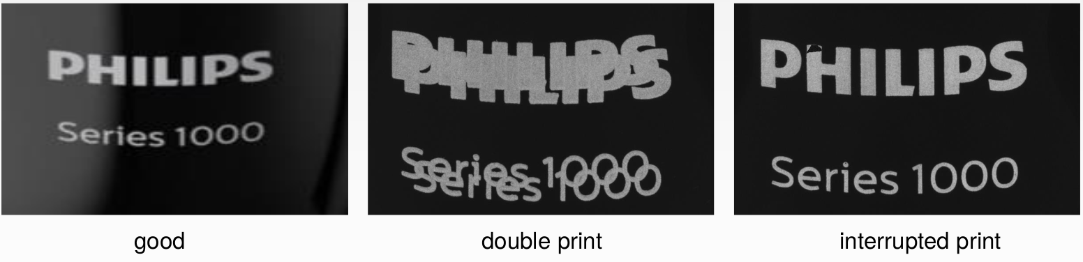
Figure 1: Sample of the Shavers dataset.

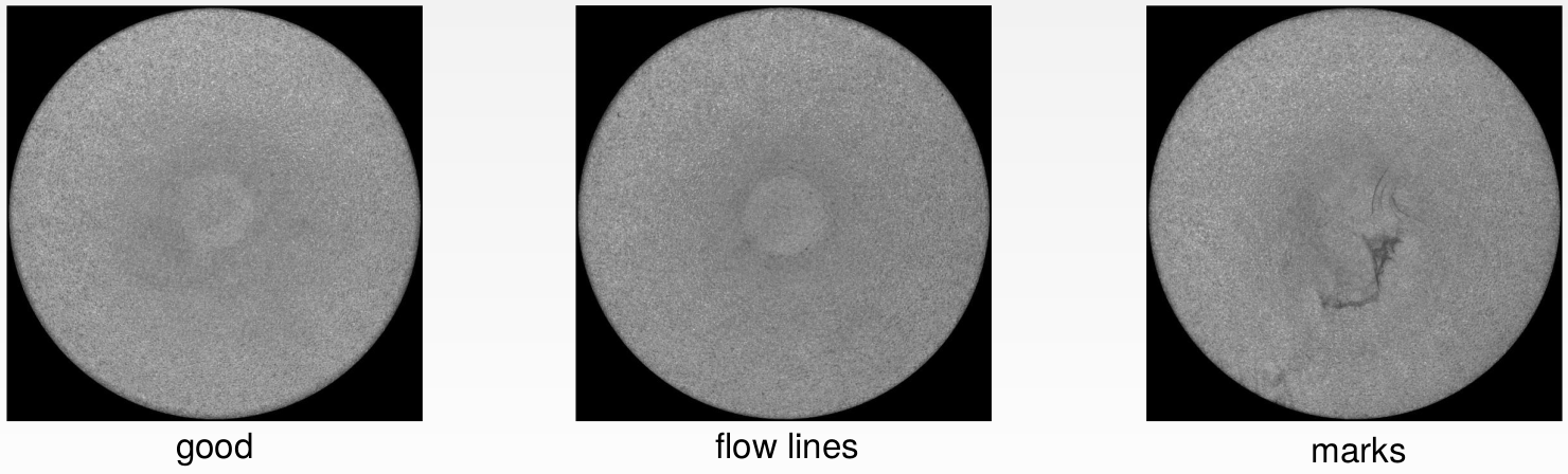
Figure 2: Sample of the Deco cap dataset.

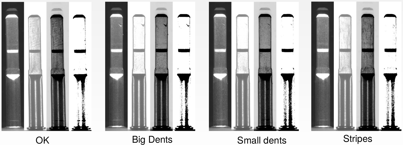
Figure 3: Sample of the Shaft dataset.

Dataset	Class	Number of examples
Deco cap	flowlines	198
	good	203
	marks	191
Shaft	big	2616
	good	528
	small	954
	stripe	151
Shavers	double	244
	good	2676
	interrupted	598

Table 1: Datasets description, describing label types and the number of data instances per label for each dataset.

4 Methodology and Experiments

In this research, we studied whether the performance of machine learning models could be enhanced, including features resulting from anomaly maps. Our intuition was that as anomaly maps highlight specific regions where defects are most likely present and help humans better decide whether a defect is present, this information could be valuable when training a machine learning model. We, therefore, studied three scenarios, training supervised machine learning models: (i) solely with the original images, (ii) only with the anomaly maps, and (iii) with features resulting from the images and anomaly maps. Furthermore, we were interested in how resilient the three types of models would be to higher class imbalance. To that end, we performed the experiments including 25%, 50%, 75%, and 100% of the images regarding defective products present in the original datasets. We consider such results relevant not only to understand the models’ resiliency but also to inform data collection and labeling efforts. If fewer defective samples are required to achieve the same performance, then data collection times could be shortened, and labeling efforts reduced.

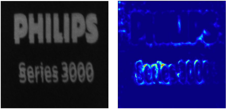
Figure 4: Image and DRAEM generated anomaly map for double print defect from Shavers dataset.

To create the anomaly maps, we trained a DRAEM model (Zavrtanik et al. (2021)), a SOTA model for unsupervised defect detection. DRAEM works by training an autoencoder on good (non-defect) images. It aims first to reconstruct artificially corrupted images to look like non-defective pieces. The original and reconstructed images are then fed to a discriminative sub-network, which identifies the anomalous regions to create an anomaly map (see Fig. 4).

We studied the machine learning models’ performance as a binary classification problem (discriminating defective from non-defective products) and a multiclass classification problem (classifying the images into particular defect categories specific to each dataset). We measured the models’ discriminative power by computing the AUC ROC metric. In the multiclass setting, we adopted the ”one-vs-rest” heuristic, computing the AUC ROC metric for each class and then computing the final value as the weighted average, considering the proportion of samples of each class in the dataset. Furthermore, we also computed two types of recall for each experiment: correct defect class recall and defect recall. Correct defect class recall indicates the percentage of defective items identified as defective considering all defective instances for the particular class being analyzed. Defect recall, on the other hand, was computed as the binary recall, considering only whether the items were identified as defective considering all defective instances, regardless the class of defect. The acceptance quality level (AQL) achieved by our models can be computed through Eq. 1.

$$AQL_{defect_{i}}=100-recall_{defect_{i}}$$ (1)

Equation 1: Equation denoting how the AQL is computed for a particular defect i.

When training the models, we performed a stratified ten-fold cross-validation (Zeng and Martinez (2000); Kuhn et al. (2013)). We used a pre-trained ResNet-18 model to extract the features from the average pool layer. To create the anomaly maps, we trained a DRAEM model on good images for each fold, using the parameters recommended by (Zavrtanik et al. (2021)).

To ensure a large number of features would not produce overfitting during training times, we performed feature selection, ranking them according to their mutual information and selecting the top K features considering $K=\sqrt{N}$, with N equal to the number of data instances in the train set (Hua et al. (2005)).

Through the experiments, we used the multi-layer perceptron (MLP) as the classifier, consisting of two dense layers (with 512 and 100 features), with an intermediate ReLU activation between both dense layers and a softmax activation at the output. We used MLP, which proved to be a good choice based on our previous work (Rozanec et al. (2022a)). We made the code available in a publicly accessible repository to promote research reproducibility . We present the results obtained and conclusions in Section 5. When assessing the results, we computed the statistical significance of the differences between the results using the Wilcoxon signed-rank test (Wilcoxon (1945)) with a p-value of $0.005$.

5 Results

This section describes the results obtained through the experiments described in Section 4. In Table 2 we inform the recall achieved for defective pieces, considering correct defect class recall, and defect recall, while in Table 3 we present results that inform the defect recall and discriminative power achieved by the defect detection models for different levels of class imbalance.

Columns under Correct defect class recall in Table 2 show the ratio between correctly identified defects versus the number of all defects of each particular class and features. Here, the results when using both image and anomaly map as the input are almost always on-par or better than the results achieved when using only image or anomaly map as the input. This demonstrates that the model benefits from additional signals introduced by the anomaly map.

The exception is the stripe class from the Shaft dataset, where all approaches struggle to differentiate this defect from others, with anomaly maps achieving the best score of $2.65\%$. Note that stripe examples are still correctly identified as defects in $95.36\%$ as achieved by the model using images and anomaly maps, they are mostly not assigned to the right class of defect.

Further, combining images and anomaly maps achieves the best results for all defect classes as seen in the columns under Defect recall in Table 2. All defects are identified for the Deco cap dataset, while scores well above $90\%$ are achieved in all other cases. Using anomaly maps alone frequently achieves better scores than using images. This is not surprising as the anomaly map shows the difference between the current and no-defect images. Any major activity in the anomaly map can be easily recognized. Here DRAEM, which is specially tailored for surface anomaly detection, learns the notion of a no-defect image, while the model has to do it in the case of images.

Detecting defects is the primary concern of visual quality inspection and is more important than classifying the defect into the right class. The acceptable performance rates are usually above $99\%$ (or less than one percent AQL), which is achieved for all but three defect classes. Here further improvements might be necessary to obtain a usable solution.

		Correct defect class recall			Defect recall
Dataset	Class	Image	Anom. map	Image + Anom. map	Image	Anom. map	Image + Anom. map
Deco cap	flowlines	98.99%	98.99%	98.99%	98.99%	100.00%	100.00%
	marks	99.48%	97.38%	98.43%	99.48%	100.00%	100.00%
Shaft	big	92.43%	87.27%	92.24%	99.73%	98.47%	99.96%
	small	59.85%	47.38%	68.03%	78.93%	90.46%	92.77%
	stripe	0.00%	2.65%	0.66%	86.75%	94.70%	95.36%
Shavers	double	97.95%	88.11%	98.36%	98.36%	96.72%	99.18%
	interrupted	84.45%	91.14%	92.64%	84.62%	92.64%	93.14%

Table 2: Percentage of images correctly classified as defects. We compute correct defect class recall (considers particular types of defects) and defect recall (binary recall - only considers defective/non-defective pieces). The best results, when statistically significant compared to the second-best results, are bolded.

Table 3 shows the classification performance on the models where a more severe imbalance of defect images is artificially introduced. The columns under Defect recall (Binary) report the recall score for defect versus no defect setting, that is, the ratio of detected defect versus all defects. The columns under ROC AUC (Multiclass) report the classification score where the defect has to be detected and assigned to the correct class. The percentage on top of each column specifies how many defect images were kept from the original dataset, with lower values resulting in a more imbalanced dataset. For example, in the first column, only $25\%$ of defect images were included in the set, while the number of good images was not reduced.

The results for Defect recall show that using images and anomaly maps is more robust for the class imbalance. On Shavers dataset, the performance drop when using only images is almost $12\%$ (absolute) when comparing the full dataset ($0.8860$ defect recall for $100\%$) with artificially imbalanced one ($0.7670$ for $25\%$). Making the same comparison, the drop in performance is only $3\%$ absolute when both images and anomaly maps are used. Similarly, the drop is smaller when using only anomaly maps than when using only images. This suggests that the anomaly maps themselves provide a strong hint and make it easier for the model to distinguish between the good images and defects from the smaller number of examples.

The results for multiclass classification in ROC AUC (Multiclass) show that using only images tends to outperform the anomaly maps, as the performance for images is higher or the difference is not significant. Although anomaly maps highlight the presence of defects on the image, they appear not fine-grained enough to successfully differentiate between the categories of defects. Combining images and anomaly maps is also the best approach in this setting.

		Defect recall (Binary)				ROC AUC (Multiclass)
Dataset	Features	25%	50%	75%	100%	25%	50%	75%	100%
Deco cap	image	0.9665	0.9922	0.9922	0.9922	0.9996	0.9997	0.9993	0.9999
	anom. map	0.9949	1.0000	1.0000	1.0000	0.9976	0.9980	0.9984	0.9985
	image + anom. map	0.9949	1.0000	1.0000	1.0000	0.9983	0.9988	0.9994	0.9996
Shaft	image	0.8417	0.9054	0.9430	0.9387	0.9146	0.9242	0.9293	0.9274
	anom. map	0.9059	0.9473	0.9629	0.9626	0.8298	0.8502	0.8585	0.8627
	image + anom. map	0.9106	0.9546	0.9669	0.9793	0.9158	0.9324	0.9388	0.9398
Shavers	image	0.7670	0.8631	0.8620	0.8860	0.9839	0.9881	0.9891	0.9897
	anom. map	0.8705	0.9039	0.9263	0.9382	0.9854	0.9899	0.9910	0.9915
	image + anom. map	0.9181	0.9465	0.9525	0.9489	0.9929	0.9949	0.9962	0.9964

Table 3: Classification results. The best results, when statistically significant compared to the second-best results, are bolded.

6 Conclusion

Based on the results, we conclude that improvement in the performance can be achieved by using both images and anomaly maps as the input to the model. Using anomaly maps also helps with the class imbalance and leads to a smaller performance drop than using only images when the imbalance is more severe. Combining the proposed approach with data imbalance mitigation techniques could lead to further improvements.

References

- Benbarrad et al. (2021) Benbarrad, T., Salhaoui, M., Kenitar, S.B., and Arioua, M. (2021). Intelligent machine vision model for defective product inspection based on machine learning. Journal of Sensor and Actuator Networks, 10(1), 7.
- Borish et al. (2019) Borish, M., Post, B.K., Roschli, A., Chesser, P.C., Love, L.J., and Gaul, K.T. (2019). Defect identification and mitigation via visual inspection in large-scale additive manufacturing. JOM, 71(3), 893–899.
- Bozic et al. (2021) Bozic, J., Tabernik, D., and Skocaj, D. (2021). Mixed supervision for surface-defect detection: From weakly to fully supervised learning. Computers in Industry, 129, 103459.
- Chin and Harlow (1982) Chin, R.T. and Harlow, C.A. (1982). Automated visual inspection: A survey. IEEE transactions on pattern analysis and machine intelligence, (6), 557–573.
- Chouchene et al. (2020) Chouchene, A., Carvalho, A., Lima, T.M., Charrua-Santos, F., Osorio, G.J., and Barhoumi, W. (2020). Artificial intelligence for product quality inspection toward smart industries: quality control of vehicle non-conformities. In 2020 9th international conference on industrial technology and management (ICITM), 127–131. IEEE.
- Chow et al. (2020a) Chow, J.K., Su, Z., Wu, J., Li, Z., Tan, P.S., Liu, K.f., Mao, X., and Wang, Y.H. (2020a). Artificial intelligence-empowered pipeline for image-based inspection of concrete structures. Automation in Construction, 120, 103372.
- Chow et al. (2020b) Chow, J.K., Su, Z., Wu, J., Tan, P.S., Mao, X., and Wang, Y.H. (2020b). Anomaly detection of defects on concrete structures with the convolutional autoencoder. Advanced Engineering Informatics, 45, 101105.
- Czimmermann et al. (2020) Czimmermann, T., Ciuti, G., Milazzo, M., Chiurazzi, M., Roccella, S., Oddo, C.M., and Dario, P. (2020). Visual-based defect detection and classification approaches for industrial applications—a survey. Sensors, 20(5), 1459.
- Deshpande et al. (2020) Deshpande, A.M., Minai, A.A., and Kumar, M. (2020). One-shot recognition of manufacturing defects in steel surfaces. Procedia Manufacturing, 48, 1064–1071.
- Escobar and Morales-Menendez (2018) Escobar, C.A. and Morales-Menendez, R. (2018). Machine learning techniques for quality control in high conformance manufacturing environment. Advances in Mechanical Engineering, 10(2), 1687814018755519.
- Garvey (2018) Garvey, C. (2018). A framework for evaluating barriers to the democratization of artificial intelligence. In Thirty-Second AAAI Conference on Artificial Intelligence.
- Glasmachers (2017) Glasmachers, T. (2017). Limits of end-to-end learning. In Asian Conference on Machine Learning, 17–32. PMLR.
- Hua et al. (2005) Hua, J., Xiong, Z., Lowey, J., Suh, E., and Dougherty, E.R. (2005). Optimal number of features as a function of sample size for various classification rules. Bioinformatics, 21(8), 1509–1515.
- Kuhn et al. (2013) Kuhn, M., Johnson, K., et al. (2013). Applied predictive modeling, volume 26. Springer.
- Long et al. (2015) Long, J., Shelhamer, E., and Darrell, T. (2015). Fully convolutional networks for semantic segmentation. In Proceedings of the IEEE conference on computer vision and pattern recognition, 3431–3440.
- Meister et al. (2021) Meister, S., Wermes, M.A., Stüve, J., and Groves, R.M. (2021). Explainability of deep learning classifier decisions for optical detection of manufacturing defects in the automated fiber placement process. In Automated Visual Inspection and Machine Vision IV, volume 11787, 1178705. International Society for Optics and Photonics.
- Peres et al. (2020) Peres, R.S., Jia, X., Lee, J., Sun, K., Colombo, A.W., and Barata, J. (2020). Industrial artificial intelligence in industry 4.0-systematic review, challenges and outlook. IEEE Access, 8, 220121–220139.
- Piciarelli et al. (2018) Piciarelli, C., Avola, D., Pannone, D., and Foresti, G.L. (2018). A vision-based system for internal pipeline inspection. IEEE Transactions on Industrial Informatics, 15(6), 3289–3299.
- Pouyanfar et al. (2018) Pouyanfar, S., Sadiq, S., Yan, Y., Tian, H., Tao, Y., Reyes, M.P., Shyu, M.L., Chen, S.C., and Iyengar, S.S. (2018). A survey on deep learning: Algorithms, techniques, and applications. ACM Computing Surveys (CSUR), 51(5), 1–36.
- Ren et al. (2021) Ren, Z., Fang, F., Yan, N., and Wu, Y. (2021). State of the art in defect detection based on machine vision. International Journal of Precision Engineering and Manufacturing-Green Technology, 1–31.
- Rozanec et al. (2022a) Rozanec, J.M., Novalija, I., Zajec, P., Kenda, K., Tavakoli Ghinani, H., Suh, S., Veliou, E., Papamartzivanos, D., Giannetsos, T., Menesidou, S.A., et al. (2022a). Human-centric artificial intelligence architecture for industry 5.0 applications. International Journal of Production Research, 1–26.
- (22) Rozanec, J.M., Zajec, P., Keizer, J., BV, P.C.L., Trajkova, E., Fortuna, B., Brecelj, B., Sircelj, B., and Mladenic, D. (????). Enhancing manual revision in manufacturing with ai-based defect hints.
- Rozanec et al. (2022b) Rozanec, J.M., Zajec, P., Trajkova, E., Sircelj, B., Brecelj, B., Novalija, I., Dam, P., Fortuna, B., and Mladenic, D. (2022b). Towards a comprehensive visual quality inspection for industry 4.0. IFAC-PapersOnLine, 55(10), 690–695.
- See (2012) See, J.E. (2012). Visual inspection: a review of the literature. Sandia Report SAND2012-8590, Sandia National Laboratories, Albuquerque, New Mexico.
- Shirvaikar (2006) Shirvaikar, M. (2006). Trends in automated visual inspection. Journal of Real-Time Image Processing, 1(1), 41–43.
- Tao et al. (2022) Tao, X., Zhang, D., Ma, W., Hou, Z., Lu, Z., and Adak, C. (2022). Unsupervised anomaly detection for surface defects with dual-siamese network. IEEE Transactions on Industrial Informatics, 18(11), 7707–7717.
- Wichmann et al. (2019) Wichmann, R.L., Eisenbart, B., and Gericke, K. (2019). The direction of industry: a literature review on industry 4.0. In Proceedings of the Design Society: International Conference on Engineering Design, volume 1, 2129–2138. Cambridge University Press.
- Wilcoxon (1945) Wilcoxon, F. (1945). Individual comparisons by ranking methods. Biometrics Bulletin, 1(6), 80–83.
- Xu et al. (2018) Xu, Z., Dang, Y., and Munro, P. (2018). Knowledge-driven intelligent quality problem-solving system in the automotive industry. Advanced Engineering Informatics, 38, 441–457.
- Zavrtanik et al. (2021) Zavrtanik, V., Kristan, M., and Skocaj, D. (2021). Draem-a discriminatively trained reconstruction embedding for surface anomaly detection. In Proceedings of the IEEE/CVF International Conference on Computer Vision, 8330–8339.
- Zeng and Martinez (2000) Zeng, X. and Martinez, T.R. (2000). Distribution-balanced stratified cross-validation for accuracy estimation. Journal of Experimental & Theoretical Artificial Intelligence, 12(1), 1–12.
- Zheng et al. (2021) Zheng, T., Ardolino, M., Bacchetti, A., and Perona, M. (2021). The applications of industry 4.0 technologies in manufacturing context: a systematic literature review. International Journal of Production Research, 59(6), 1922–1954.