On the string topology of symmetric spaces of higher rank

Abstract.

The homology of the free and the based loop space of a compact globally symmetric space can be studied through explicit cycles. We use cycles constructed by Bott and Samelson and by Ziller to study the string topology coproduct and the Chas-Sullivan product on compact symmetric spaces. We show that the Chas-Sullivan product for compact symmetric spaces is highly non-trivial for any rank and we prove that there are many non-nilpotent classes whose powers correspond to the iteration of closed geodesics. Moreover, we show that the based string topology coproduct is trivial for compact symmetric spaces of higher rank and we study the implications of this result for the string topology coproduct on the free loop space. We explicitly study the product of two even-dimensional spheres and show that the string topology coproduct is trivial in this case.

1. Introduction

String topology is the study of algebraic structures on the homology or cohomology of the free loop space $\Lambda M$ of a closed manifold $M$. The most prominent operation is the Chas-Sullivan product which is a product of the form

$$\wedge\colon\mathrm{H}_{i}(\Lambda M)\otimes\mathrm{H}_{j}(\Lambda M)\to\mathrm{H}_{i+j-n}(\Lambda M)$$

where $n$ is the dimension of the underlying oriented manifold $M$. This product was first introduced by Chas and Sullivan in [CS99] via geometric intersections of chains in the free loop space. The geometric idea of the Chas-Sullivan product is to concatenate loops which share the same basepoint. It turns out that the Chas-Sullivan product only depends on the homotopy type of $M$, see [CKS08].

Since the influential paper by Chas and Sullivan [CS99] many more string topology operations have been studied. In particular we want to mention the operation induced by the $\mathbb{S}^{1}$-action on the free loop space which together with the Chas-Sullivan product induces the structure of a Batalin-Vilkovisky algebra on the homology of the free loop space, see [CS99, Theorem 5.4].

In [GH09] Goresky and Hingston introduce the string topology coproduct which is a map

$$\vee\colon\mathrm{H}_{i}(\Lambda M,M)\to\mathrm{H}_{i+1-n}(\Lambda M\times\Lambda M,\Lambda M\times M\cup M\times\Lambda M)\,.$$

Here we consider $M$ as a subset of the free loop space via the identification of $M$ with the trivial loops in $M$. The idea for this coproduct goes back to Sullivan, see [Sul04]. Geometrically, the coproduct looks for loops with self-intersections and cuts them apart at the basepoint. In certain situations the string topology coproduct induces a dual product in cohomology, the Goresky-Hingston product which takes the form

$$\mathbin{\mathchoice{\ooalign{$\displaystyle\vbox{\hbox{\scalebox{0.77778}{$\displaystyle\bigcirc$}}}$\cr$\displaystyle\ast$\cr}}{\ooalign{$\textstyle\vbox{\hbox{\scalebox{0.77778}{$\textstyle\bigcirc$}}}$\cr$\textstyle\ast$\cr}}{\ooalign{$\scriptstyle\vbox{\hbox{\scalebox{0.77778}{$\scriptstyle\bigcirc$}}}$\cr$\scriptstyle\ast$\cr}}{\ooalign{$\scriptscriptstyle\vbox{\hbox{\scalebox{0.77778}{$\scriptscriptstyle\bigcirc$}}}$\cr$\scriptscriptstyle\ast$\cr}}}\colon\mathrm{H}^{i}(\Lambda M,M)\otimes\mathrm{H}^{j}(\Lambda M,M)\to\mathrm{H}^{i+j+n-1}(\Lambda M,M)\,.$$

Hingston and Wahl further study the string topology coproduct and the Goreky-Hingston product in [HW17]. In [Nae21] Naef shows that the string topology coproduct is not a homotopy invariant in general. This is further examined in [NRW22]. However, if the underlying manifold $M$ is simply connected, then the string topology coproduct only depends on the homotopy type of $M$, see [HW19]. There is also a coproduct on the based loop space of the manifold $M$

$$\vee_{\Omega}\colon\mathrm{H}_{i}(\Omega M,\{p_{0}\})\to\mathrm{H}_{i+1-n}(\Omega M\times\Omega M,\Omega M\times\{p_{0}\}\cup\{p_{0}\}\times\Omega M)$$

which is strongly related to the string topology coproduct.

From a geometric point of view the homology of the free loop space is very important in the study of closed geodesics in a closed Riemannian manifold $(M,g)$. It turns out that the critical points of the energy functional $E\colon\Lambda M\to\mathbb{R}$ given by

$$E(\gamma)=\frac{1}{2}\int_{0}^{1}g_{\gamma(s)}(\dot{\gamma}(s),\dot{\gamma}(s))\,\mathrm{d}s,\quad\gamma\in\Lambda M\,,$$

are precisely the closed geodesics in $M$ with respect to the metric $g$. Morse-theoretic methods therefore give a connection between the topology of $\Lambda M$ and the closed geodesics in $M$.

The connection between string topology and closed geodesics has been studied in a few instances. Hingston and Rademacher [HR13] use explicit computations of the Chas-Sullivan and the Goresky-Hingston product on spheres to prove a resonance property of closed geodesics. Goresky and Hingston [GH09] define Chas-Sullivan and Goresky-Hinston type products in the level homologies and cohomologies of the free loop space and compute these products for spheres and projective spaces. In particular, they then use the level products to compute the Chas-Sullivan and the Goresky-Hingston product for spheres, see [GH09, Section 15]. Moreover, Goresky and Hingston show that for spheres and projective spaces there are non-nilpotent classes for both products and that the powers of these classes corresponds to the iteration of the closed geodesics. We also refer to [HW17] for a computation of the string topology coproduct on odd-dimensional spheres. Goresky and Hingston use the well understood geometry of a metric where all geodesics are closed and of the same length for their computation of the string topology products. Note that the standard examples for such metrics are the compact symmetric spaces of rank one.

It is natural to ask how the string topology operations behave for arbitrary compact globally symmetric spaces of higher rank. In this article we use explicit cycles in the based and the free loop space, respectively, of a compact symmetric space which were introduced by Bott and Samelson [BS58] and by Ziller [Zil77]. While the Chas-Sullivan and the Goresky-Hingston product have been studied for compact symmetric spaces of rank $1$, these operations have not yet been studied extensively for compact symmetric spaces of higher rank which are not Lie groups. In the rank $1$ case, we mentioned above the computations for spheres by Goresky and Hingston [GH09] and Hingston and Wahl [HW17]. Furthermore, the Chas-Sullivan product has been computed for complex projective spaces in [CJY03] and for quaternionic projective spaces and the Cayley plane in [CM10]. A product induced by the Chas-Sullivan product on the quotient of $\Lambda\mathbb{S}^{n}$ by the action generated by orientation reversal of loops has been computed by the first author in [Kup21]. The Goresky-Hingston product for complex and quaternionic projective spaces has been studied in [Ste22b]. The string topology of compact Lie groups has been studied by Hepworth [Hep09] and the second author [Ste22a]. The second author shows in [Ste22a] that the string topology coproduct is trivial for compact simply connected Lie groups of rank $r\geq 2$.

In the present article we study the Chas-Sullivan product for compact symmetric spaces using Ziller’s explicit cycles. Let $\gamma$ be a closed geodesic and let $\Sigma_{\gamma}\subseteq\Lambda M$ be the critical manifold containing $\gamma$. There is a compact manifold $\Gamma_{\gamma}$, which, as we shall see later, we understand as a completing manifold for $\Sigma_{\gamma}$. The manifold $\Gamma_{\gamma}$ fibers over $\Sigma_{\gamma}$ and embeds into the free loop space via a map $f_{\gamma}\colon\Gamma_{\gamma}\hookrightarrow\Lambda M$. If we take $\mathbb{Z}_{2}$-coefficients we take the orientation class of $\Gamma_{\gamma}$ and we consider the class $(f_{\gamma})_{*}[\Gamma_{\gamma}]\in\mathrm{H}_{*}(\Lambda M)$.

Theorem (Theorem 5.3).

Let $M$ be a compact symmetric space and take homology with $\mathbb{Z}_{2}$-coefficients. For every critical manifold $\Sigma_{\gamma}$ the associated class $(f_{\gamma})_{*}[\Gamma_{\gamma}]$ is non-nilpotent in the Chas-Sullivan algebra and the powers of this class correspond to the iteration of the closed geodesics. More precisely, if $m_{1},m_{2}\in\mathbb{N}$ we have

$$(f_{\gamma^{m_{1}}})_{*}[\Gamma_{\gamma^{m_{1}}}]\wedge(f_{\gamma^{m_{2}}})_{*}[\Gamma_{\gamma^{m_{2}}}]=(f_{\gamma^{m_{1}+m_{2}}})_{*}[\Gamma_{\gamma^{m_{1}+m_{2}}}]\,.$$

This theorem shows that the Chas-Sullivan product of compact symmetric spaces of higher rank is highly non-trivial. In particular, we argue that if the rank $r$ of the compact symmetric space $M$ satisfies $r\geq 2$, then there are infinitely many critical manifolds consisting of prime closed geodesics, each of which induces a non-nilpotent homology class. We also show that the Chas-Sullivan product of classes associated to a critical manifold $\Sigma_{\gamma^{m_{1}}}$ and classes associated to $\Sigma_{\gamma^{m_{2}}}$ is strongly related to the intersection product in the manifold $\Sigma\cong\Sigma_{\gamma^{m_{1}}}\cong\Sigma_{\gamma^{m_{2}}}$. See Theorem 5.5 for details.

Furthermore, we study the string topology coproduct on the based loop space of a compact symmetric space as well as the coproduct on the corresponding free loop space.

Theorem (Corollary 6.4 and Proposition 6.9).

Let $M$ be a compact simply connected symmetric space of rank greater than or equal to $2$.

1. The based coproduct $\vee_{\Omega}$ on the homology of the based loop space $\mathrm{H}_{*}(\Omega M,p_{0};\mathbb{Z}_{2})$ is trivial.

2. To every non-trivial critical manifold $\Sigma\subseteq\Lambda M$ of the energy functional one can associate a homology class $[W_{\Sigma}]\in\mathrm{H}_{\mathrm{ind}(\Sigma)}(\Lambda M,M;\mathbb{Z}_{2})$ which has trivial string topology coproduct.

Note that this result shows that the Goresky-Hingston product behaves quite differently when one compares compact symmetric spaces of rank $1$ and of higher rank, since in the rank $1$ case the dual of the class $[W_{\Sigma}]$ in cohomology is non-nilpotent in the Goresky-Hingston algebra. In contrast to this, our results for the Chas-Sullivan product show that the Chas-Sullivan product for higher rank symmetric spaces behaves very similarly to the rank $1$ case.

Furthermore, we show that for a product of compact symmetric spaces the string topology coproduct vanishes on a large subspace of the homology of the free loop space.

Theorem (Theorem 7.3).

Let $M=M_{1}\times M_{2}$ be a product of two compact symmetric spaces. Let $U$ denote the subspace of $\mathrm{H}_{*}(\Lambda M,M;\mathbb{Z}_{2})$ generated by the classes induced by completing manifolds associated to critical manifolds $\Sigma=\Sigma_{1}\times\Sigma_{2}$ where both $\Sigma_{1}$ and $\Sigma_{2}$ consist of non-constant closed geodesics. Then the string topology coproduct vanishes on $U$.

Finally, we study the string topology coproduct on the product of two even-dimensional spheres. We prove the following result.

Theorem (Theorem 7.8).

Let $M=\mathbb{S}^{2m}\times\mathbb{S}^{2n}$ be a product of two even-dimensional spheres. Then the string topology coproduct on $M$ is trivial with rational coefficients.

This article is organized as follows. In Section 2 we introduce the Chas-Sullivan product and the string topology coproduct. The notion of a completing manifold, which is the central idea behind Bott and Samelson’s and Ziller’s cycles, is studied in Section 3. In Section 4 we give an overview over the geodesics in compact symmetric spaces and set the ground for the definition of the explicit cycles in the loop spaces of compact symmetric spaces in the following sections. In Section 5 we study Ziller’s cycles in detail and show how they can be used to compute the Chas-Sullivan product. We use Bott’s and Samelson’s cycles in Section 6 to study the string topology coproduct on the based and on the free loop space. Finally, in Section 7 we show the triviality of the string topology coproduct on products of even-dimensional spheres by studying the explicit Ziller cycles in this case.

2. String topology product and coproduct

In this section we introduce the string topology operations which we examine in this article. We follow [GH09] for the definition of the Chas-Sullivan product and [HW17] for the definition of the string topology coproduct.

Let $(M,g)$ be a closed Riemannian manifold of dimension $n$. We denote the unit interval by $I=[0,1]$. We define the path space of $M$ to be

$$PM=\big{\{}\gamma:I\to M\,|\,\gamma\,\,\text{absolutely continuous},\,\,\int_{0}^{1}g_{\gamma(t)}(\dot{\gamma}(t),\dot{\gamma}(t))\,\mathrm{d}t<\infty\big{\}}\,.$$

We refer to [Kli95, Definition 2.3.1] for the definition of absolute continuity of curves in a smooth manifold. It turns out that the path space $PM$ can be given the structure of a Hilbert manifold, see [Kli95, Section 2.3]. The free loop space of $M$ is defined to be the subspace

$$\Lambda M=\{\gamma\in PM\,|\,\gamma(0)=\gamma(1)\}$$

which is in fact a submanifold of $PM$. The underlying manifold $M$ can be seen as a submanifold of $\Lambda M$ via the identification with the trivial loops, see [Kli78, Proposition 1.4.6]. We consider the energy functional

$$E^{\prime}:PM\to[0,\infty),\qquad E^{\prime}(\gamma)=\frac{1}{2}\int_{0}^{1}g_{\gamma(t)}(\dot{\gamma}(t),\dot{\gamma}(t))\mathrm{d}t\,.$$

This is a smooth function on the path space $PM$, see [Kli95, Theorem 2.3.20]. By restriction we obtain the energy functional on the free loop space which we will denote by $E=E^{\prime}|_{\Lambda M}$. The critical points of $E$ on $\Lambda M\smallsetminus M$ are precisely the closed geodesics in $M$. Moreover, for a point $p_{0}\in M$ we define

$$\Omega_{p_{0}}M=\{\gamma\in\Lambda M\,|\,\gamma(0)=p_{0}\}$$

and call this space the based loop space of $M$ at the point $p_{0}$. The based loop space is a submanifold of the free loop space $\Lambda M$. Note that we will also frequently write $\Lambda$ for the free loop space $\Lambda M$ and $\Omega M$ or $\Omega$ for the based loop space if the manifold or the basepoint, respectively, are fixed. In the following let $R$ be a commutative ring with unit and consider homology and cohomology with coefficients in $R$. We assume that the manifold $M$ is oriented with respect to the coefficients $R$. If $\epsilon>0$ is smaller than the injectivity radius of $M$, then the diagonal $\Delta M\subseteq M\times M$ has a tubular neighborhood

$$U_{M}\coloneqq\{(p,q)\in M\times M\,|\,\mathrm{d}(p,q)<\epsilon\}\,.$$

Here, $\mathrm{d}$ is the distance function on $M$ induced by the Riemannian metric. Note that the normal bundle of $M\cong\Delta M$ in the product $M\times M$ is isomorphic to the tangent bundle $TM$. Consequently, since $U_{M}$ is a tubular neighborhood there is a homeomorphism of pairs

$$(U_{M},U_{M}\smallsetminus M)\cong(TM,TM\smallsetminus M)\,.$$

If we pull back the Thom class of $(TM,TM\smallsetminus M)$ via this homeomorphism we obtain a class

$$\tau_{M}\in\mathrm{H}^{n}(U_{M},U_{M}\smallsetminus M)\,.$$

On the free loop space $\Lambda M$ we consider the evaluation map $\mathrm{ev}_{0}\colon\Lambda\to M$ given by

$$\mathrm{ev}_{0}(\gamma)=\gamma(0)\,.$$

We define the figure-eight space $\Lambda\times_{M}\Lambda$ as the pull-back

$$\Lambda\times_{M}\Lambda=(\mathrm{ev}_{0}\times\mathrm{ev}_{0})^{-1}(\Delta M)=\{(\gamma,\sigma)\in\Lambda\times\Lambda\,|\,\gamma(0)=\sigma(0)\}\,.$$

It turns out that the pull-back of the tubular neighborhood of the diagonal $U_{M}$ yields a tubular neighborhood of the figure-eight space

$$U_{CS}\coloneqq(\mathrm{ev}_{0}\times\mathrm{ev}_{0})^{-1}(U_{M})=\{(\gamma,\sigma)\in\Lambda\times\Lambda\,|\,\mathrm{d}(\gamma(0),\sigma(0))<\epsilon\}\,,$$

see e.g. [HW17]. One can now pull back the Thom class $\tau_{M}$ via the map $\mathrm{ev}_{0}\times\mathrm{ev}_{0}$ to obtain a class

$$\tau_{CS}\coloneqq(\mathrm{ev}_{0}\times\mathrm{ev}_{0})^{*}\tau_{M}\in\mathrm{H}^{n}(U_{CS},U_{CS}\smallsetminus\Lambda\times_{M}\Lambda)\,.$$

Let $R\colon U_{CS}\to\Lambda\times_{M}\Lambda$ be the retraction of the tubular neighborhood. Furthermore, for a time $s\in(0,1)$ there is a concatenation map

$$\mathrm{concat}_{s}\colon\Lambda\times_{M}\Lambda\to\Lambda$$

given by

$$\mathrm{concat}_{s}(\gamma,\sigma)(t)\coloneqq\begin{cases}\gamma(\tfrac{t}{s}),&0\leq t\leq s\\ \sigma(\tfrac{t-s}{1-s}),&s\leq t\leq 1\,.\end{cases}$$

Note that for $s,t\in(0,1)$ the maps $\mathrm{concat}_{s}$ and $\mathrm{conact}_{t}$ are homotopic via re-parametrization. Thus, for the induced map in homology, we just write $\mathrm{concat}_{*}$. We can now define the Chas-Sullivan product.

Definition 2.1.

Let $M$ be a closed $R$-oriented $n$-dimensional manifold. The Chas-Sullivan product is defined as the composition

$$\wedge\colon\mathrm{H}_{i}(\Lambda)\otimes\mathrm{H}_{j}(\Lambda) \xrightarrow{(-1)^{n(n-j)}\times} \mathrm{H}_{i+j}(\Lambda\times\Lambda)$$

$$\xrightarrow{\hphantom{coninci}\vphantom{r}\hphantom{conci}} \mathrm{H}_{i+j}(\Lambda\times\Lambda,\Lambda\times\Lambda\smallsetminus\Lambda\times_{M}\Lambda)$$

$$\xrightarrow{\hphantom{cii}\text{excision}\hphantom{ici}} \mathrm{H}_{i+j}(U_{CS},U_{CS}\smallsetminus\Lambda\times_{M}\Lambda)$$

$$\xrightarrow{\hphantom{coci}\tau_{CS}\cap\hphantom{coci}} \mathrm{H}_{i+j-n}(U_{CS})$$

$$\xrightarrow[]{\hphantom{conci}R_{*}\hphantom{conci}} \mathrm{H}_{i+j-n}(\Lambda\times_{M}\Lambda)$$

$$\xrightarrow[]{\hphantom{ici}\mathrm{concat}_{*}\hphantom{ici}} \mathrm{H}_{i+j-n}(\Lambda\times\Lambda)\,.$$

Remark 2.2.

The Chas-Sullivan product is an associative, graded commutative and unital product, see e.g. [GH09]. Moreover, it only depends on the homotopy type of the underlying manifold $M$, see [CKS08].

We now turn to the definition of the string topology coproduct. Recall that we had the explicit tubular neighborhood of the diagonal $U_{M}$. Let $\epsilon_{0}>0$ be a small positive number with $\epsilon_{0}<\epsilon$ and define

$$U_{M,\geq\epsilon_{0}}=\{(p,q)\in U_{M}\,|\,\mathrm{d}(p,q)\geq\epsilon_{0}\}\,.$$

Note that by [HW17] the pair $(U_{M},U_{M,\geq\epsilon_{0}})$ is homeomorphic to $(TM^{<\epsilon},TM^{<\epsilon}_{\geq\epsilon_{0}})$ where

$$TM^{<\epsilon}\coloneqq\{v\in TM\,|\,|v|<\epsilon\}\quad\text{and}\quad TM^{<\epsilon}_{\geq\epsilon_{0}}\coloneqq\{v\in TM^{<\epsilon}\,|\,|v|\geq\epsilon_{0}\}$$

and where $|\cdot|$ is the fiberwise norm induced by the Riemannian metric on $M$. Moreover, by [HW17] the Thom class in $(TM,TM\smallsetminus M)$ induces a Thom class in $(TM^{\epsilon},TM^{<\epsilon}_{\geq\epsilon_{0}})$. Consequently, we obtain a class $\tau_{M}^{\prime}\in\mathrm{H}^{n}(U_{M},U_{M,\geq\epsilon_{0}})$. Fix a basepoint $p_{0}\in M$ and consider the sets

$$B_{p_{0}}\coloneqq\{q\in M\,|\,\mathrm{d}(p_{0},q)<\epsilon\}\quad\text{and}\quad B_{p_{0},\geq\epsilon_{0}}\coloneqq\{q\in B_{p_{0}}\,|\,\mathrm{d}(p_{0},q)\geq\epsilon_{0}\}\,.$$

Let $i$ be the inclusion

$$i\colon B_{p_{0}}\xrightarrow[]{\cong}\{p_{0}\}\times B_{p_{0}}\hookrightarrow U_{M}\,.$$

This induces a map of pairs $j\colon(B_{p_{0}},B_{p_{0},\geq\epsilon_{0}})\to(U_{M},U_{M,\geq\epsilon_{0}})$. If we pull back the class $\tau_{M}^{\prime}$ via this map we obtain a class

$$\tau_{p_{0}}\coloneqq j^{*}\tau_{M}^{\prime}\in\mathrm{H}^{n}(B_{p_{0}},B_{p_{0},\geq\epsilon_{0}})\cong\mathrm{H}(M,M\smallsetminus\{p_{0}\})$$

and by the properties of a Thom class this class coincides with the generator of $\mathrm{H}(M,M\smallsetminus\{p_{0}\})$ induced by the orientation of $M$.

On the product of the free loop space with the unit interval $\Lambda\times I$ there is an evaluation map

$$\mathrm{ev}_{I}\colon\Lambda\times I\to M\times M$$

given by

$$\mathrm{ev}_{I}(\gamma,s)=(\gamma(0),\gamma(s))\,.$$

Define

$$U_{GH}=(\mathrm{ev}_{I})^{-1}(U_{M})=\{(\gamma,s)\in\Lambda M\times I\,|\,\mathrm{d}(\gamma(0),\gamma(s))<\epsilon\}$$

and

$$U_{GH,\geq\epsilon_{0}}=(\mathrm{ev}_{I})^{-1}(U_{M,\geq\epsilon_{0}})=\{(\gamma,s)\in U_{GH}\,|\,\mathrm{d}(\gamma(0),\gamma(s))\geq\epsilon_{0}\}\,.$$

The set $U_{GH}$ is an open neighborhood of the subspace

$$F_{GH}\coloneqq(\mathrm{ev}_{I})^{-1}(\Delta M)=\{(\gamma,s)\in\Lambda\times I\,|\,\gamma(0)=\gamma(s)\}\,.$$

The evaluation $\mathrm{ev}_{I}$ defines a map of pairs

$$\mathrm{ev}_{I}\colon(U_{GH},U_{GH,\geq\epsilon_{0}})\to(U_{M},U_{M,\geq\epsilon_{0}})$$

and we can pull back the class $\tau_{M}^{\prime}$ to obtain a class

$$\tau_{GH}\coloneqq(\mathrm{ev}_{I})^{*}\tau_{M}^{\prime}\in\mathrm{H}^{n}(U_{GH},U_{GH,\geq\epsilon_{0}})\,.$$

The above constructions can be done similarly for the based loop space, i.e. we obtain an open neighborhood $U^{\Omega}_{GH}=U_{GH}\cap(\Omega\times I)$ of the space

$$F^{\Omega}_{GH}\coloneqq F_{GH}\cap(\Omega\times I)=\{(\gamma,s)\in\Omega\times I\,|\,\gamma(s)=p_{0}\}$$

and we pull back the class $\tau_{p_{0}}$ to a class

$$\tau^{\Omega}_{GH}\in\mathrm{H}^{n}(U^{\Omega}_{GH},U^{\Omega}_{GH,\geq\epsilon_{0}})$$

where $U^{\Omega}_{GH,\geq\epsilon_{0}}\coloneqq U_{GH,\geq\epsilon_{0}}\cap(\Omega\times I)$.

As Hingston and Wahl argue in [HW17] there is a retraction map $R_{GH}\colon U_{GH}\to F_{GH}$ and it is easy to see that this restricts to a retraction $U_{GH}^{\Omega}\to F^{\Omega}_{GH}$. Furthermore, we have a cutting map $\mathrm{cut}\colon F_{GH}\to\Lambda\times\Lambda$ given by

$$\mathrm{cut}(\gamma,s)=(\gamma|_{[0,s]},\gamma|_{[s,1]})$$

where by $\gamma|_{[0,s]}$ we mean a reparametrized version of the restriction $\gamma|_{[0,s]}$. Again, this restricts appropriately to a based version.

Let $[I]$ be the positively oriented generator of $\mathrm{H}_{1}(I,\partial I)$ with respect to the standard orientation of the unit interval. We write $p_{0}$ for the basepoint of the based loop space which is just the trivial loop at the point $p_{0}$ and by abuse of notation we shall denote the set consisting of the single element $p_{0}$ just by $p_{0}$.

Definition 2.3.

Let $M$ be a closed $R$-oriented manifold of dimension $n$.

1. The string topology coproduct is defined as the map

   $$\vee:\mathrm{H}_{*}(\Lambda,M) \xrightarrow{\hphantom{oi}\times[I]\hphantom{oi}} \mathrm{H}_{*+1}(\Lambda\times I,\Lambda\times\partial I\cup M\times I)$$

   $$\xrightarrow{\hphantom{o}\tau_{GH}\cap\hphantom{o}} \mathrm{H}_{*+1-n}(U_{GH},\Lambda\times\partial I\cup p_{0}\times I)$$

   $$\xrightarrow{(\mathrm{R}_{GH})_{*}} \mathrm{H}_{*+1-n}(F_{GH},\Lambda\times\partial I\cup M\times I)$$

   $$\xrightarrow{\hphantom{i}(\mathrm{cut})_{*}\hphantom{i}} \mathrm{H}_{*+1-n}(\Lambda\times\Lambda,\Lambda\times M\cup M\times\Lambda)\,.$$

2. The based string topology coproduct is defined as the map

   $$\vee_{\Omega}:\mathrm{H}_{*}(\Omega,p_{0}) \xrightarrow{\hphantom{oi}\times[I]\hphantom{oi}} \mathrm{H}_{*+1}(\Omega\times I,\Omega\times\partial I\cup p_{0}\times I)$$

   $$\xrightarrow{\hphantom{o}\tau_{GH}^{\Omega}\cap\hphantom{o}} \mathrm{H}_{*+1-n}(U_{GH}^{\Omega},\Omega\times\partial I\cup p_{0}\times I)$$

   $$\xrightarrow{(\mathrm{R}_{GH})_{*}} \mathrm{H}_{*+1-n}(F^{\Omega}_{GH},\Omega\times\partial I\cup p_{0}\times I)$$

   $$\xrightarrow{\hphantom{i}(\mathrm{cut})_{*}\hphantom{i}} \mathrm{H}_{*+1-n}(\Omega\times\Omega,\Omega\times p_{0}\cup p_{0}\times\Omega)\,.$$

Remark 2.4.

If we take $R=\mathbb{F}$ to be a field, then by the Künneth isomorphism the string topology coproduct induces a map

$$\vee^{\prime}\colon\mathrm{H}_{i}(\Lambda,M)\to(\mathrm{H}_{*}(\Lambda,M)\otimes\mathrm{H}_{*}(\Lambda,M))_{i+1-n}\,.$$

After a sign correction this map is indeed coassociative and graded cocommutative, see [HW17, Theorem 2.14] and therefore justifies the name coproduct.

Note that the based string topology coproduct and the string topology coproduct on the free loop space are compatible with respect to the inclusion $i\colon\Omega\hookrightarrow\Lambda$. More precisely, we have the commutativity of the following diagram, see [Ste22a, Proposition 2.4].

If the homology $\mathrm{H}_{*}(\Lambda,M)$ is of finite type, then the coproduct with coefficients in a field induces a product in cohomology.

Definition 2.5.

Let $\mathbb{F}$ be a field and assume that the homology of $\Lambda M$ is of finite type. Let $\alpha\in\mathrm{H}^{i}(\Lambda,M;\mathbb{F})$ and $\beta\in\mathrm{H}^{j}(\Lambda,M;\mathbb{F})$ be relative cohomology classes, then the Goresky-Hingston product $\alpha\mathbin{\mathchoice{\ooalign{$\displaystyle\vbox{\hbox{\scalebox{0.77778}{$\displaystyle\bigcirc$}}}$\cr$\displaystyle\ast$\cr}}{\ooalign{$\textstyle\vbox{\hbox{\scalebox{0.77778}{$\textstyle\bigcirc$}}}$\cr$\textstyle\ast$\cr}}{\ooalign{$\scriptstyle\vbox{\hbox{\scalebox{0.77778}{$\scriptstyle\bigcirc$}}}$\cr$\scriptstyle\ast$\cr}}{\ooalign{$\scriptscriptstyle\vbox{\hbox{\scalebox{0.77778}{$\scriptscriptstyle\bigcirc$}}}$\cr$\scriptscriptstyle\ast$\cr}}}\beta$ is defined to be the unique cohomology class in $\mathrm{H}^{i+j+n-1}(\Lambda,M;\mathbb{F})$ such that

$$\langle\alpha\mathbin{\mathchoice{\ooalign{$\displaystyle\vbox{\hbox{\scalebox{0.77778}{$\displaystyle\bigcirc$}}}$\cr$\displaystyle\ast$\cr}}{\ooalign{$\textstyle\vbox{\hbox{\scalebox{0.77778}{$\textstyle\bigcirc$}}}$\cr$\textstyle\ast$\cr}}{\ooalign{$\scriptstyle\vbox{\hbox{\scalebox{0.77778}{$\scriptstyle\bigcirc$}}}$\cr$\scriptstyle\ast$\cr}}{\ooalign{$\scriptscriptstyle\vbox{\hbox{\scalebox{0.77778}{$\scriptscriptstyle\bigcirc$}}}$\cr$\scriptscriptstyle\ast$\cr}}}\beta,X\rangle=\langle\alpha\times\beta,\operatorname{\vee}X\rangle\qquad\text{for all}\,\,\,X\in\mathrm{H}_{*}(\Lambda M,M;\mathbb{F})\,.$$

We conclude this section by defining the intersection multiplicity of a relative homology class for both the based loop space and the free loop space. Hingston and Wahl define the notion of basepoint intersection multiplicity in [HW17, Section 5] only in the case free loop space. The analogous concept for the based loop space is straight-forward.

Definition 2.6.

Let $M$ be a closed manifold with basepoint $p_{0}\in M$.

1. Let $[X]\in\mathrm{H}_{*}(\Lambda M,M;R)$ be a homology class with representing cycle $X\in\mathrm{C}_{*}(\Lambda M,M)$. Assume that the relative cycle $X$ is itself represented by a cycle $x\in\mathrm{C}_{*}(\Lambda M)$. The intersection multiplicity $\mathrm{int}([X])$ of the class $[X]$ is the number

   $$\mathrm{int}([X])\coloneqq\inf_{A\sim x}\Big{(}\sup\big{[}\#(\gamma^{-1}(\{p_{0}\}))\,|\,\gamma\in\mathrm{im}(A),\,\,\,E(\gamma)>0\big{]}\Big{)}-1$$

   where the infimum is taken over all cycles $A\in\mathrm{C}_{*}(\Lambda M)$ homologous to $x$.

2. Let $[X]\in\mathrm{H}_{*}(\Omega_{p_{0}}M,p_{0};R)$ be a homology class with representing cycle $X\in\mathrm{C}_{*}(\Omega_{p_{0}}M,p_{0})$. Assume that the relative cycle $X$ is itself represented by a cycle $x\in\mathrm{C}_{*}(\Omega_{p_{0}}M)$. The intersection multiplicity $\mathrm{int}([X])$ of the class $[X]$ is the number

   $$\mathrm{int}([X])\coloneqq\inf_{A\sim x}\Big{(}\sup\big{[}\#(\gamma^{-1}(\{p_{0}\}))\,|\,\gamma\in\mathrm{im}(A),\,\,\,E(\gamma)>0\big{]}\Big{)}-1$$

   where the infimum is taken over all cycles $A\in\mathrm{C}_{*}(\Omega_{p_{0}}M)$ homologous to $x$.

By considering finite-dimensional models of $\Lambda M$, respectively of $\Omega_{p_{0}}M$, one sees that the intersection multiplicity of a homology class is finite. Hingston and Wahl prove in the case of the free loop space that if a homology class $Y\in\mathrm{H}_{*}(\Lambda M,M)$ has intersection multiplicity $1$ then its coproduct vanishes, see [HW17, Theorem 3.10]. Since the proof of this theorem which includes Lemma 3.5 and Proposition 3.6 of [HW17] only uses maps that keep the basepoint of the loops fixed, the proof can be transferred directly to the case of the based loop space. We obtain the following result.

Proposition 2.7 ([HW17], Theorem 3.10).

Let $M$ be a closed manifold with basepoint $p_{0}\in M$ and let $R$ be a commutative ring. Assume that $M$ is $R$-oriented.

1. Suppose that $[X]\in\mathrm{H}_{*}(\Lambda M,M;R)$ has intersection multiplicity $\mathrm{int}([X])=1$, then the string topology coproduct $\operatorname{\vee}[X]$ vanishes.

2. Suppose that $[X]\in\mathrm{H}_{*}(\Omega_{p_{0}}M,p_{0};R)$ has intersection multiplicity $\mathrm{int}([X])=1$, then the based coproduct $\operatorname{\vee}_{\Omega}[X]$ vanishes.

3. Completing manifolds

In this section we introduce the concept of a completing manifold. This will be the key technique in our study of the string topology operations on symmetric spaces in Sections 6 and 5. We closely follow [HO13] and [Oan15].

Assume that $X$ is a Hilbert manifold and that $F\colon X\to\mathbb{R}$ is a Morse-Bott function. Let $a$ be a critical value of $F$ and assume that the set of critical points at level $a$ is non-degenerate submanifold $\Sigma$ with index $\lambda$ and with orientable negative bundle. As usual in Morse theory we denote by $X^{\leq a}$ the set

$$X^{\leq a}\coloneqq\{x\in X\,|\,F(x)\leq a\}\,.$$

Similarly, one defines the strict sublevel set $X^{<a}$. It is well-known that the level homology $\mathrm{H}_{*}(X^{\leq a},X^{<a})$ is completely determined by the homology of the critical manifold $\Sigma$. More precisely, we have

$$\mathrm{H}_{*}(X^{\leq a},X^{<a})\cong\mathrm{H}_{*-\lambda}(\Sigma)\,.$$

In general, there is no direct link between the homology of $\Sigma$ and the homology of the sublevel set $X^{\leq a}$. As we shall see in the following the existence of a completing manifold however is sufficient for the property that the homology of $X^{\leq a}$ is a direct sum of the homology of the strict sublevel set $X^{<a}$ and the homology of the critical manifold $\Sigma$.

Definition 3.1.

Let $X$ be a Hilbert manifold and let $F\colon X\to\mathbb{R}$ be a Morse-Bott function. Suppose that $a$ is a critical value of $F$ and assume that $\Sigma$ is the oriented non-degenerate critical submanifold at level $a$ of index $\lambda$ and of dimension $m=\mathrm{dim}(\Sigma)$. A completing manifold for $\Sigma$ is a closed, orientable manifold $\Gamma$ of dimension $\lambda+m$ with a closed submanifold $S$ of codimension $\lambda$. Moreover, there is a map $f:\Gamma\to X^{\leq a}$ such that the following holds. The map $f$ is an embedding near $S$ with the restriction $f|_{S}$ mapping $S$ homeomorphically onto $\Sigma$ and such that $f^{-1}(\Sigma)=S$. Furthermore, there is a retraction map $p:\Gamma\to S$ and the map $f$ induces a map of pairs

$$f\colon(\Gamma,\Gamma\smallsetminus S)\to(X^{\leq a},X^{<a})\,.$$

In case that we consider homology with $\mathbb{Z}_{2}$-coefficients we drop the orientability conditions on $\Sigma$ and $\Gamma$.

Remark 3.2.

Note that the above definition is the one of a strong completing manifold in [Oan15]. Since in the present article we only encounter this stronger version of a completing manifold, we just call it completing manifold. Furthermore, we remark that in the present article all maps $f\colon\Gamma\to X$ from the completing manifold $\Gamma$ to the Hilbert manifold $X$ will be embeddings so that the property of being an embedding near $S$ is clearly satisfied.

Let $g\colon M\to N$ be a map between compact oriented manifolds. We recall that the Gysin map

$$g_{!}\colon\mathrm{H}_{i}(N)\to\mathrm{H}_{i+\mathrm{dim}(M)-\mathrm{dim}(N)}(M)$$

is defined by

$$g_{!}\colon\mathrm{H}_{i}(N)\xrightarrow[]{(PD_{N})^{-1}}\mathrm{H}^{\mathrm{dim}(N)-i}(N)\xrightarrow[]{g^{*}}\mathrm{H}^{\mathrm{dim}(N)-i}(M)\xrightarrow[]{PD_{M}}\mathrm{H}_{\mathrm{dim}(M)-(\mathrm{dim}(N)-i)}(M),$$

where

$$\mathrm{PD}_{L}\colon\mathrm{H}^{j}(L)\xrightarrow[]{\cong}\mathrm{H}_{\mathrm{dim}(L)-j}(L)$$

stands for Poincaré duality on the compact oriented manifold $L$. In particular, we note that Gysin maps behave contravariantly, i.e. if $h\colon N\to L$ is a second map between compact oriented manifolds, then

$$(h\circ g)_{!}=g_{!}\circ h_{!}\,.$$ (3.1)

If we use $\mathbb{Z}_{2}$-coefficients then all orientability conditions in the above can be dropped.

Let $X$ be a Hilbert manifold with a Morse-Bott function $F\colon X\to\mathbb{R}$. Assume that $\Sigma$ is an oriented critical submanifold at level $a$ and that $\Gamma$ is a completing manifold for $\Sigma$. Then we have the embedded submanifold $s\colon S\hookrightarrow\Gamma$ and if $p\colon\Gamma\to S$ is the retraction we clearly have

$$p\circ s=\operatorname{id}_{S}\,.$$ (3.2)

Moreover, note that we get a map

$$\mathrm{H}_{i}(\Gamma)\to\mathrm{H}_{i}(\Gamma,\Gamma\smallsetminus S)\xrightarrow[]{\cong}\mathrm{H}_{i-\lambda}(S)$$

where the first map is induced by the inclusion of pairs and the second one is made up by excision and the Thom isomorphism. It turns out, see [Bre13, Theorem 11.3], that this map coincides up to sign with the Gysin map $s_{!}$. Consequently, by equations (3.1) and (3.2) we see that $p_{!}$ is a right inverse to this map up to sign. In particular, the long exact sequence of the pair $(\Gamma,\Gamma\smallsetminus S)$ yields a short exact sequence in each degree which splits via the map $p_{!}$. Thus, for each $i\in\mathbb{N}$ we have a short exact sequence

$$0\to\mathrm{H}_{i}(\Gamma\smallsetminus S)\to\mathrm{H}_{i}(\Gamma)\xrightarrow[]{s_{!}}\mathrm{H}_{i-\lambda}(S)\to 0$$

and due to the splitting $p_{!}$ we see that

$$\mathrm{H}_{i}(\Gamma)\cong\mathrm{H}_{i}(\Gamma\smallsetminus S)\oplus\mathrm{H}_{i-\lambda}(S)\cong\mathrm{ker}(s_{!})\oplus\mathrm{H}_{i-\lambda}(S)\cong\mathrm{ker}(s_{!})\oplus\mathrm{im}(p_{!})\,.$$

Combining these ideas with the map $f\colon\Gamma\to X$ one can show the following.

Proposition 3.3 ([Oan15], Lemma 6.2).

Let $X$ be a Hilbert manifold, $F\colon X\to\mathbb{R}$ a Morse-Bott function and let $a$ be a critical value of $F$. Assume that the set of critical points at level $a$ is an oriented non-degenerate critical submanifold $\Sigma$ of index $\lambda$. If there is a completing manifold for $\Sigma$ then

$$\mathrm{H}_{*}(X^{\leq a})\cong\mathrm{H}_{*}(X^{<a})\oplus\mathrm{H}_{*}(X^{\leq a},X^{<a})\cong\mathrm{H}_{*}(X^{<a})\oplus\mathrm{H}_{*-\lambda}(\Sigma)\,.$$ (3.3)

Remark 3.4.

Note that the construction of a completing manifold does not only give us the isomorphism of Proposition 3.3, but it also yields an explicit way of describing the homology classes which come from the critical manifold $\Sigma$. More precisely, by the above discussion it is clear that the composition

$$f_{*}\circ p_{!}\colon\mathrm{H}_{i}(\Sigma)\to\mathrm{H}_{i+\lambda}(\Gamma)\to\mathrm{H}_{i+\lambda}(X^{\leq a})$$

is injective. Here, the map $f$ is the map of the completing manifold $\Gamma$ into $X$ and $p$ is the retraction $\Gamma\to S\cong\Sigma$.

Recall that the homology of the completing manifold $\Gamma$ splits as

$$\mathrm{H}_{i}(\Gamma)\cong\mathrm{H}_{i}(\Gamma\smallsetminus S)\oplus\mathrm{H}_{i}(\Gamma,\Gamma\smallsetminus S)\cong\mathrm{H}_{i}(\Gamma\smallsetminus S)\oplus\mathrm{H}_{i-\lambda}(\Sigma)\,.$$

We note that while we usually only care about the classes in $\mathrm{H}_{i}(\Gamma)$ that are in the image of $p_{!}\colon\mathrm{H}_{i}(\Sigma)\to\mathrm{H}_{i+\lambda}(\Gamma)$, we cannot say much about the image of $\mathrm{H}_{i}(\Gamma\smallsetminus S)$ under the map $f_{*}$. For example, it is not clear in general when a class in $\mathrm{H}_{i}(\Gamma\smallsetminus S)$ lies in the kernel of $f_{*}$. However, by the commutativity of the diagram

we do see that $\mathrm{H}_{i}(\Gamma\smallsetminus S)$ is mapped to the homology of the strict sublevel set $\mathrm{H}_{i}(X^{<a})$ via $f_{*}$.

If $X$ is a Hilbert manifold with a Morse-Bott function $F\colon X\to\mathbb{R}$ let us assume that for every critical value $a$ we have

$$\mathrm{H}_{*}(X^{\leq a})\cong\mathrm{H}_{*}(X^{<a})\oplus\mathrm{H}_{*}(X^{\leq a},X^{<a})\,.$$ (3.4)

In this case we say that the function $F$ is a perfect Morse-Bott function. This property clearly holds if every critical submanifold is oriented and has a completing manifold. Ziller shows in [Zil77] that the energy functional on the free loop space of a compact symmetric space is perfect if one takes $\mathbb{Z}_{2}$-coefficients. He uses explicit completing manifolds which we shall study in detail in Section 5 in order to compute the Chas-Sullivan product on symmetric spaces partially.

4. Geodesics in symmetric spaces

In this section we review some standard constructions in the theory of globally symmetric spaces. In Sections 5 and 6 we shall use the concepts of this present section and therefore want to introduce the necessary tools in a concise manner. A general reference for the geometry of symmetric spaces is [Hel78].

Let $M=G/K$ be a compact symmetric space where $(G,K)$ is a symmetric pair. Note that we always assume $M$ to be connected and that we always choose $G$ to be connected. There is an involution $\sigma\colon G\to G$ such that $\sigma\neq\mathrm{id}_{G}$ and such that

$$\mathrm{Fix}(\sigma)_{0}\subseteq K\subseteq\mathrm{Fix}(\sigma)\,.$$

Here $\mathrm{Fix}(\sigma)$ means the subgroup of $K$ consisting of elements which are fixed by $\sigma$, i.e.

$$\mathrm{Fix}(\sigma)=\{k\in G\,|\,\sigma(k)=k\}\,.$$

Moreover, by the subscript $0$ we denote the connected component of the unit element $e\in G$. Let $\mathfrak{g}\cong T_{e}G$ be the Lie algebra of $G$. The differential $\mathrm{D}\sigma_{e}$ is an involutive Lie algebra automorphism of $\mathfrak{g}$ and therefore $\mathfrak{g}$ has a decomposition of the form

$$\mathfrak{g}=\mathfrak{k}\oplus\mathfrak{m}\,,$$

with

$$\mathfrak{k}=\mathrm{Eig}(\mathrm{D}\sigma_{e},+1)\quad\text{and}\quad\mathfrak{m}=\mathrm{Eig}(\mathrm{D}\sigma_{e},-1)\,.$$

Note that $\mathfrak{k}$ is a Lie subalgebra of $\mathfrak{g}$ and that $[\mathfrak{m},\mathfrak{m}]\subseteq\mathfrak{k}$. Moreover, the subgroup $K$ acts on $\mathfrak{m}$ via the adjoint action, i.e.

$$\mathrm{Ad}|_{K\times\mathfrak{m}}\colon K\times\mathfrak{m}\to\mathfrak{m}\,,$$

where $\mathrm{Ad}\colon G\times\mathfrak{g}\to\mathfrak{g}$ is the adjoint action of $G$. If $\pi\colon G\to M=G/K$ is the canonical projection then

$$\mathrm{D}\pi_{e}|_{\mathfrak{m}}\colon\mathfrak{m}\to T_{o}M$$

is an isomorphism where $o=\pi(e)\in M$. Consider the complexification $\mathfrak{g}_{\mathbb{C}}$ of $\mathfrak{g}$. There exists a Cartan subalgebra $\mathfrak{h}\subseteq\mathfrak{g}_{\mathbb{C}}$, see [Hel78, p. 284]. In particular a Cartan subalgebra is abelian. A root of $\mathfrak{g}_{\mathbb{C}}$ is a non-zero element $\alpha$ of the dual space $\mathfrak{h}^{*}$ such that there is a non-trivial element $X\in\mathfrak{g}_{\mathbb{C}}$ with

$$[H,X]=\pi\,i\,\alpha(H)X\quad\text{for all}\,\,\,H\in\mathfrak{h}\,.$$

We denote the set of roots of $\mathfrak{g}_{\mathbb{C}}$ by $\Delta^{\prime}$. There is a maximal abelian subalgebra $\mathfrak{a}$ of $\mathfrak{m}$ such that $\mathfrak{a}$ is contained in the Cartan subalgebra $\mathfrak{h}$, see [Hel78, p. 284]. We call the subspace $\mathfrak{a}$ a Cartan subalgebra of $(G,K)$. Note that the rank of $M$ is equal to the dimension of $\mathfrak{a}$. Let $\Delta$ be the set of roots $\alpha\in\Delta^{\prime}$ such that $\alpha|_{\mathfrak{a}}\neq 0$ where we identify two roots $\alpha_{1},\alpha_{2}\in\Delta^{\prime}$ if $\alpha_{1}|_{\mathfrak{a}}=\alpha_{2}|_{\mathfrak{a}}$. One can define an ordering on the set of roots and define the set of positive roots $\Delta_{+}\subseteq\Delta$, see [Hel78, Section VII.2] for details. Then the positive Weyl chamber of $\Delta$ can be defined as

$$W:=\{X\in\mathfrak{a}\,|\,\alpha(X)>0\text{ for all }\alpha\in\Delta_{+}\}.$$

Note that the other Weyl chambers arise by different choices of the positive roots. The Weyl group $W(G,K)$ of the symmetric pair $(G,K)$ is generated by the reflections $s_{\alpha}$ on the hyperplanes

$$\{H\in\mathfrak{a}\,|\,\alpha(H)=0\}\,.$$

The Weyl group is a finite group and acts simply transitively on the set of Weyl chambers. Finally, we define the map $\mathrm{Exp}\colon\mathfrak{m}\to M$ by

$$\mathrm{Exp}=\pi\circ\mathrm{exp}|_{\mathfrak{m}}$$

with $\mathrm{exp}$ being the Lie group exponential. It turns out that this map is in fact the Riemannian exponential map at the point $o$ under the canonical identification $T_{o}M\cong\mathfrak{m}$. Set $T=\mathrm{Exp}(\mathfrak{a})$ which is a flat totally geodesic submanifold of maximal dimension, often called the maximal torus even in cases when $M$ is not a Lie group. In particular, the geodesics in $T$ are just the images of the straight lines in $\mathfrak{a}$ under the exponential map $\mathrm{Exp}$.

We now want to see what the roots tell us about the geometry of $M$. Consider a pair $(\alpha,n)$ where $\alpha\in\Delta$ and $n\in\mathbb{Z}$. This defines an affine hyperplane

$$\{H\in\mathfrak{a}\,|\,\alpha(H)=n\}\subseteq\mathfrak{a}$$

which we call a singular plane and which we denote by $(\alpha,n)$. The geodesics in $T$ starting at $o$ are images of lines through the origin in $\mathfrak{a}$ under $\mathrm{Exp}$. Let

$$\sigma_{H}\colon[0,\infty)\to\mathfrak{a},\quad\sigma_{H}(t)=tH$$

for some $H\in\mathfrak{a}$ be such a ray and let

$$\gamma_{H}\colon[0,\infty)\to M,\quad\gamma_{H}=\operatorname{Exp}\circ\,\sigma_{H}$$

be the corresponding geodesic in $M$. Define times $0=t_{0}<t_{1}<t_{2}<\ldots$ inductively by setting $t_{0}=0$ and

$$t_{i}\coloneqq\inf\{t\in(t_{i-1},\infty)\,|\,\sigma(t)\text{ lies in a hyperplane }(\alpha,n),\,\,n\neq 0\}$$

for $i\geq 1$. Of course, it is also possible that $\sigma$ meets an intersection of several hyperplanes at a time $t_{i}$, $i\in\mathbb{N}$. The following Proposition states that the singular planes encode the conjugate points in the symmetric space $M$.

Proposition 4.1 ([Hel78], Proposition VII.3.1).

Let $\sigma_{H}$ and $\gamma_{H}$ be defined as above and consider the set $C=\{t_{i}\}_{i\in\mathbb{N}}$. The point $\gamma(t)$ is conjugate to $o$ along $\gamma$ if and only if $t\in C$.

We refer to Figure 1 for a sketch of the singular planes of a symmetric space of rank $2$. A priori Proposition 4.1 is only a statement about the geodesics in $M$ which start at $o$ and which lie in the maximal torus $T$. However, the following proposition shows that every geodesic $\gamma\colon[0,\infty)\to M$ is isometric to one of the form $\gamma_{H}$ as above. Note that the action of $G$ on the symmetric space $M$ induces an action on the free loop space $\Phi\colon G\times\Lambda M\to\Lambda M$ given by

$$\Phi(g,\gamma)(t)\coloneqq g.\gamma(t)\quad\text{for}\,\,g\in G,\gamma\in\Lambda M\,.$$

Proposition 4.2.

Let $\gamma\colon[0,\infty)\to M$ be a geodesic in $M$. Then there is an isometry $g\in\mathrm{Isom}(M)_{0}$ and an element $H\in\mathfrak{a}$ such that $g.\gamma=\gamma_{H}$.

This follows from the theorems about maximal tori in symmetric spaces, see e.g. [Hel78, Proposition VII.2.2] and the discussion in [Zil77, p. 6]. Let $\mathcal{F}\subseteq\mathfrak{a}$ be the lattice defined by

$$\mathcal{F}=\{H\in\mathfrak{a}\,|\,\operatorname{Exp}(H)=o\}\,.$$

It is clear that the closed geodesics in the maximal torus $T$ are in one-to-one correspondence to the lattice $\mathcal{F}$. See Figure 1 for a sketch of the lattice of a symmetric space of rank $2$.

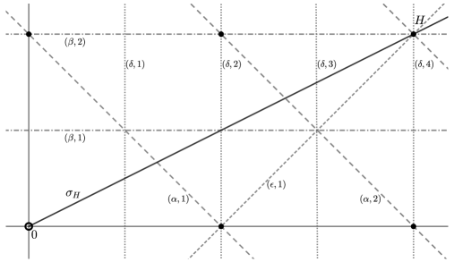
Figure 1. Maximal abelian subspace of a symmetric space of rank $2$. There are four positive roots $\{\alpha,\beta,\delta,\epsilon\}$ and the corresponding singular planes are drawn as dashed or dotted lines. The lattice points are pictured as dots. The ray $\sigma_{H}$ is mapped to a closed geodesic by $\operatorname{Exp}$ since it intersects the lattice $\mathcal{F}$ at the point $H$. Observe that there are five conjugate points in the interior of the corresponding closed geodesic $\gamma_{H}$. They can be read off by considering the intersections of $\sigma_{H}$ with the singular planes. The above figure shows the maximal abelian subspace for the complex Grassmannian $\mathrm{Gr}_{2}(\mathbb{C}^{4})$, see [Sak77, Section 4.2] and [Sak78, Example 5.5].

By the above we see that the critical submanifolds of the energy functional in $\Lambda M$ are the orbits of the closed geodesics in $T$ under the action of $G$. However, note that several distinct points in the lattice $\mathcal{F}$ can correspond to closed geodesics which lie in the same orbit under the action of $G$. In order to get a one-to-one correspondence between points in the lattice $\mathcal{F}$ and the critical submanifolds, we need to consider the intersection of the lattice $\mathcal{F}$ with the closure of the Weyl chamber $\overline{W}$. Recall that we call a closed geodesic $\gamma\in\Lambda M$ prime if it is not the iterate of another closed geodesic, i.e. if there is no $l\geq 2$ and a closed geodesic $\sigma\in\Lambda M$ with $\gamma=\sigma^{l}$. We say that a critical submanifold is prime if it consists only of prime closed geodesics. We sum up the above considerations in the following proposition.

Proposition 4.3.

The critical manifolds of the energy functional in the free loop space are in one-to-one correspondence with the set $\mathcal{F}\cap\overline{W}$. In particular, if the rank of $M$ satisfies $r\geq 2$ there are countably infinite distinct prime critical submanifolds.

Proof.

The first part of the proposition is contained in [Zil77]. If the rank of $M$ satisfies $r\geq 2$ then the lattice is generated by elements $X_{1},\ldots,X_{r}$. Every element of the form

$$\lambda_{1}X_{1}+\ldots+\lambda_{r}X_{r}\quad\text{with at least one }\lambda_{i}=\pm 1,\,\,i\in\{1,\ldots,r\}$$ (4.1)

corresponds to a prime closed geodesic. If $r\geq 2$ there are clearly countably infinite such elements. Recall that all Weyl chambers are homeomorphic and that the union of the closures of the finitely many Weyl chambers is all of $\mathfrak{a}$. Since the action of the Weyl group preserves the lattice $\mathcal{F}$, see [Hel78, Proof of Theorem 8.5], there must be countably infinite elements of the form of equation (4.1) in each Weyl chamber. ∎

Recall from Section 3 that the energy function $E\colon\Lambda M\to\mathbb{R}$ of a symmetric metric is a perfect Morse-Bott function, see [Zil77]. We conclude this section by computing the index growth of the closed geodesics. Let $c$ be a closed geodesic in $M$ starting at the basepoint $o$, not necessarily of the form $\gamma_{H}$ as above. Let $K_{c}$ be the closed subgroup of $K$ that keeps $c$ pointwise fixed, i.e.

$$K_{c}=\{k\in K\,|\,k.c(t)=c(t)\,\,\text{for all}\,\,t\in I\}\,.$$

One can show that $q=c(t)\in M$ is a conjugate point along $c$, $t\in I$, if and only if the stabilizer

$$K_{q}\coloneqq\{k\in K\,|\,k.q=q\}$$

of $q$ satisfies

$$\mathrm{dim}(K_{q})>\mathrm{dim}(K_{c})\,,$$

see [Zil77, p. 14]. Moreover, the difference $\mathrm{dim}(K_{q})-\mathrm{dim}(K_{c})$ is precisely the multiplicity of the conjugate point $q$. Furthermore, one shows that the index of the closed geodesic $c$ is equal to the sum of the multiplicities of the conjugate points in the interior, see [Zil77, Theorem 4]. This means that we have

$$\mathrm{ind}(c)=\sum_{0<t_{i}<1}(\mathrm{dim}(K_{c(t_{i})})-\mathrm{dim}(K_{c}))\,,$$

where the times $t_{i}\in(0,1)$ are such that $c(t_{i})$ is a conjugate point as above. Define the integer $\mu=\mathrm{dim}(K)-\mathrm{dim}(K_{c})$. If $c$ is the $k$-th iterate of a prime closed geodesics $\sigma$, then by a simple counting argument we obtain

$$\mathrm{ind}(c)=k\,\mathrm{ind}(\sigma)+(k-1)\mu$$ (4.2)

since the origin appears $(k-1)$ times in the interior of $c$ and clearly has stabilizer $K$.

Finally, the nullity of the closed geodesic $c$, i.e. the dimension of the kernel of the hessian of $E$ at $c$, is equal to the dimension of the homogeneous space $G/K_{c}$, since $G/K_{c}$ is the non-degenerate critical submanifold containing $c$ of the Morse-Bott function $E$, see [Zil77]. Since the canonical map

$$G/K_{c}\to G/K,\quad gK_{c}\mapsto gK$$

is a fiber bundle with typical fiber $K/K_{c}$, we see that

$$\mathrm{null}(c)=\mathrm{dim}(G/K)+\mathrm{dim}(K/K_{c})=n+\mu\,.$$

Consequently, the sum of index and nullity of the $k$-th iterate of a prime closed geodesic $\sigma$ is

$$(\mathrm{ind}+\mathrm{null})(c)=k\,\mathrm{ind}(\sigma)+k\,\mu+n\,.$$ (4.3)

Remark 4.4.

Note that the homogeneous space $K/K_{c}$ is diffeomorphic to the orbit $K.c\subseteq\Omega M$ of the closed geodesic $c$ under the induced action of $K$ on the based loop space. Moreover, note that one can also identify $K_{c}$ with the subgroup

$$\{k\in K\,|\,\mathrm{Ad}_{k}(\dot{c}(0))=\dot{c}(0)\}\subseteq K\,,$$

see [Zil77, p. 14]. The group $K$ acts by linear isometries on the space $\mathfrak{m}$, hence the orbit of $\dot{c}(0)$ is diffeomorphic to the space $K/K_{c}$ which is embedded in the hypersphere

$$S_{c}\coloneqq\{X\in\mathfrak{m}\,|\,|X|=|\dot{c}(0)|\}\cong\mathbb{S}^{n-1}\,.$$

Recall that the dimension of $K/K_{c}$ is $\mu$. As usual we can assume that $\dot{c}(0)\in\mathfrak{a}$.

If $M$ is an $n$-dimensional symmetric space of rank $1$, then the space $K/K_{c}$ is diffeormorphic to the sphere $\mathbb{S}^{n-1}$, since the compact rank one symmetric spaces are precisely the symmetric spaces where all geodesics are closed and of common prime length. If $M$ is $n$-dimensional and of rank $r\geq 2$, then the orbit of $K$ cannot be the whole hypersphere, which one can see as follows. If the orbit of $K$ was the whole $S_{c}$ then in particular every point in $S_{c}\cap\mathfrak{a}$ lies in the orbit $K.\dot{c}(0)$. But if $H\in\mathfrak{a}$ is in the $K$-orbit of $\dot{c}(0)$, i.e. there is a $k\in K$ with $H=\mathrm{Ad}_{k}(\dot{c}(0))$ then it is well-known that there is an element of the Weyl group $s\in W(G,K)$ with $H=s(\dot{c}(0))$. But there are only finitely many elements of the Weyl group, so for rank $r\geq 2$ this yields a contradiction to the assumption that the $K$-orbit of $\dot{c}(0)$ is all of $S_{c}$. Consequently, $K/K_{c}$ is an embedded submanifold of $\mathbb{S}^{n-1}$ which is not the whole sphere and therefore must have positive codimension. This shows that $\mu$ must be strictly smaller than $n-1$.

5. The Chas-Sullivan product on symmetric spaces

Let $M=G/K$ be a compact symmetric space with $(G,K)$ being a Riemannian symmetric pair as in Section 4. In this section we are going to show that for each critical submanifold $\Sigma\subseteq\Lambda M$ consisting of prime closed geodesics of $M$, there is a non-nilpotent element in the Chas-Sullivan algebra of $\Lambda M$. While in the case of a rank one symmetric space there is only one such homology class, in higher rank cases there are infinitely many. The rank one case follows from Section 13 of [GH09]. We extend the result therein to the higher rank case using completing manifolds, which avoids discussing level homologies.

In this section our unital coefficient ring $R$ for homology and cohomolgy is always chosen such that all critical and completing manifolds are $R$-orientable. In most cases this means that we take $R=\mathbb{Z}_{2}$ since we do not have a general answer to the question whether all critical and all completing manifolds of a given symmetric space are orientable. As before the coefficient ring is omitted from the notation in what follows.

Let $\gamma$ be a closed geodesic in $M$. Recall from Section 4 that there is an element $g\in G$ and an isometric closed geodesic $c$ such that $c=g.\gamma$ satisfies $c(0)=o$. Therefore the critical manifold of $c$ in $\Lambda M$ with respect to the energy functional is diffeomorphic to $\Sigma_{c}=G/K_{c}$ where $K_{c}$ is the isotropy group

$$K_{c}\coloneqq\{k\in K\,|\,k.c(t)=c(t)\,\,\text{for all}\,\,t\in[0,1]\}\subseteq K\,.$$

The projection $\Sigma_{c}=G/K_{c}\to G/K$ is a fibre bundle projection

$$K/K_{c}\hookrightarrow\Sigma_{c}\xrightarrow[]{\pi}M$$

with homogeneous fibre $K/K_{c}$.

We shall now describe Ziller’s explicit cycles which are completing manifolds for the critical manifolds $\Sigma_{c}$. It will be apparent that they are closely related to Bott’s $K$-cycles. Fix a closed geodesic $c\in\Lambda M$ with $c(0)=o$. Again from Section 4 we recall the following: If $q\in M$ is a point we denote its stabilizer under the action of $K$ by $K_{q}$, i.e.

$$K_{q}=\{k\in K\,|\,k.q=q\}\,.$$

As Ziller [Zil77] and Bott and Samelson [BS58] argue there are finitely many times $0<t_{1}<\ldots<t_{l}<1$ such that $\mathrm{dim}(K_{c(t_{i})})>\mathrm{dim}(K_{c})$ for $i\in\{1,\ldots,l\}$. The points $c(t_{i})$, $i\in\{1,\ldots,l\}$ are precisely the conjugate points along $c$ and the multiplicity of such a conjugate point is equal to $\mathrm{dim}(K_{c(t_{i})})-\mathrm{dim}(K_{c})$. Moreover the Morse index of the closed geodesic $c$ can be expressed as

$$\mathrm{ind}(c)=\sum_{i=1}^{l}\big{(}\mathrm{dim}(K_{c(t_{i})})-\mathrm{dim}(K_{c})\big{)}\,.$$

If $c$ has multiplicity $m$, i.e. there is an underlying prime closed geodesic $\sigma$ with $c=\sigma^{m}$, then it holds that $c(\tfrac{j}{m})=o$ for $j\in\{1,\ldots,m-1\}$ and the corresponding stabilizer is the whole group $K$. Define $\mu\coloneqq\mathrm{dim}(K)-\mathrm{dim}(K_{c})$. Recall from Section 4 that the index of the iterates of $\sigma$ equals

$$\mathrm{ind}(c)=\mathrm{ind}(\sigma^{m})=m\mathrm{ind}(\sigma)+(m-1)\mu\,.$$

Moreover we have

$$\mathrm{dim}(\Sigma_{c})=n+\mu\,,$$

where $n$ is the dimension of $M$. We consider the product of groups

$$W_{c}\coloneqq G\times K_{c(t_{1})}\times K_{c(t_{2})}\times\ldots\times K_{c(t_{l})}\,.$$

There is a right-action of the $(l+1)$-fold product of $K_{c}$ on $W_{c}$ given by

$$\chi:W_{c}\times K_{c}^{l+1} \to W_{c}$$ (5.1)

$$((g_{0},k_{1},\ldots,k_{l}),(h_{0},\ldots,h_{l})) \mapsto (g_{0}h_{0},h_{0}^{-1}k_{1}h_{1},\ldots,h_{l-1}^{-1}k_{l}h_{l})\,.$$

This is a proper and free action and we denote the quotient by

$$\Gamma_{c}\coloneqq W_{c}/(K_{c}^{l+1})\,.$$

Note that there is a submersion

$$p\colon\Gamma_{c}\to\Sigma_{c}\cong G/K_{c}\,,\quad p([(g_{0},k_{1},\ldots,k_{l})])=[g_{0}]\,.$$ (5.2)

Furthermore there is an embedding $\Sigma_{c}\to\Gamma_{c}$ defined by

$$s\colon\Sigma_{c}\to\Gamma_{c}\,,\quad s([g])=[(g,e,\ldots,e)]$$

and one sees that $p\circ s=\mathrm{id}_{\Sigma_{c}}$.

We now describe an embedding $\Gamma_{c}\hookrightarrow\Lambda M$. Define $\widetilde{f}_{c}\colon W_{c}\to\Lambda M$ by

$$\widetilde{f}_{c}(g_{0},k_{1},\ldots,k_{l})(t)=\begin{cases}g_{0}.c(t),&0\leq t\leq t_{1}\\ g_{0}k_{1}.c(t),&t_{1}\leq t\leq t_{2}\\ \,\,\,\,\,\vdots&\,\,\,\,\,\vdots\\ g_{0}k_{1}\ldots k_{l}.c(t),&t_{l}\leq t\leq 1\,\,\,.\end{cases}$$

This factors through the action of $K_{c}^{l+1}$ and therefore defines a map $f_{c}\colon\Gamma_{c}\to\Lambda M$. It can be seen directly that this is an embedding and that $f_{c}\circ s\colon\Sigma_{c}\to\Lambda M$ embeds $\Sigma_{c}$ precisely as the critical manifold. Moreover, the only closed geodesics in $f_{c}(\Gamma_{c})$ are in this critical manifold. Hence, we see that $\Gamma_{c}$ is a completing manifold if coefficients are taken in $\mathbb{Z}_{2}$. The same is true with $R$-coefficients if $\Sigma_{c}$ and $\Gamma_{c}$ are $R$-orientable as follows from Section 3. An explicit example of these completing manifolds for even-dimensional spheres and products of even-dimensional spheres is studied in detail in Section 7.

We now show that Ziller’s cycles behave well with respect to the concatenation map

$$\mathrm{concat}_{s}\colon\Lambda\times_{M}\Lambda\to\Lambda\,,\quad(\gamma_{1},\gamma_{2})\mapsto\gamma\,,$$

where $s\in(0,1)$ and where

$$\gamma(t)\coloneqq\begin{cases}\gamma_{1}(\tfrac{t}{s})&0\leq t\leq s\\ \gamma_{2}(\tfrac{t+s}{1-s})&s\leq t\leq 1\,\,\,.\end{cases}$$

Let $\sigma\in\Lambda M$ be a prime closed geodesic and suppose that $\gamma_{1},\gamma_{2}\in\Lambda M$ are iterates of $\sigma$ with multiplicities $m_{1}$ and $m_{2}$. Just as above one can set up completing manifolds $\Gamma_{1}$ and $\Gamma_{2}$ corresponding to the critical manifolds $\Sigma_{1}$ and $\Sigma_{2}$ where $\Sigma_{i}\subseteq\Lambda M$ is the critical manifold containing $\gamma_{i}$ for $i\in\{1,2\}$. We want to study the relation between $\Gamma_{1},\Gamma_{2}$ and the completing manifold $\Gamma_{3}$ associated to the concatenation $\gamma_{3}=\sigma^{m_{1}+m_{2}}$. We set $m_{3}=m_{1}+m_{2}$ and note that we have

$$\Sigma_{3}\cong\Sigma_{1}\cong\Sigma_{2}\cong G/K_{\sigma}\,.$$

Recall that we have submersions $p_{i}\colon\Gamma_{i}\to\Sigma_{i}$, $i\in\{1,2,3\}$, and that there is a fiber bundle $\pi\colon G/K_{\sigma}\to M$. This gives submersions $\pi\circ p_{i}\colon\Gamma_{i}\to M$ and we can look at the fiber product

$$\Gamma_{1}\times_{M}\Gamma_{2}\subseteq\Gamma_{1}\times\Gamma_{2}$$

with respect to $\pi\circ p_{1}$ and $\pi\circ p_{2}$. Clearly, $\Gamma_{1}\times_{M}\Gamma_{2}$ is a submanifold of $\Gamma_{1}\times\Gamma_{2}$ of codimension $n$ and it has a canonical map

$$p_{1}\times p_{2}\colon\Gamma_{1}\times_{M}\Gamma_{2}\to\Sigma_{1}\times_{M}\Sigma_{2},\quad(p_{1}\times p_{2})(X,Y)=(p_{1}(X),p_{2}(Y))\,.$$

Moreover, we see that

$$\Gamma_{1}\times_{M}\Gamma_{2}=\{([(g_{0},k_{1},\ldots,k_{l_{1}})],[(\widetilde{g}_{0},\widetilde{k}_{1},\ldots,\widetilde{k}_{l_{2}})])\in\Gamma_{1}\times\Gamma_{2}\,|\,g_{0}K=\widetilde{g}_{0}K\}\,.$$ (5.3)

Recall the construction of the group $W_{c}$ above for a closed geodesic $c$. If we define $H$ by $W_{\sigma}=G\times H$ where $\sigma$ is the underlying prime closed geodesic of $\gamma_{1}$ and $\gamma_{2}$ as before, then we see that

$$W_{\gamma_{i}}=G\times H\times(K\times H)^{m_{i}-1}\,,\quad i\in\{1,2,3\}\,.$$

Define a map $\Phi\colon\Gamma_{1}\times_{M}\Gamma_{2}\to\Gamma_{3}$ by

$$\Phi([(g_{0},k_{1},\ldots,k_{l_{1}})],[(\widetilde{g}_{0},\widetilde{k}_{1},\ldots,\widetilde{k}_{l_{2}})])=[(g_{0},k_{1},\ldots,k_{l_{1}},(g_{0}k_{1}\ldots k_{l_{1}})^{-1}\widetilde{g}_{0},\widetilde{k}_{1},\ldots,\widetilde{k}_{l_{2}})].$$

Note that the map $\Phi$ is smooth and indeed well-defined since $g_{0}^{-1}\widetilde{g}_{0}\in K$ by equation (5.3). Set $\tau=\tfrac{m_{1}}{m_{1}+m_{2}}$ and define $\phi\colon\Sigma_{1}\times_{M}\Sigma_{2}\to\Sigma_{3}$ by

$$\phi([g],[\widetilde{g}])=[g]$$

where we identify $\Sigma_{i}\cong G/K_{\sigma}$ as usual.

Lemma 5.1.

The map $\Phi$ is a diffeomorphism. Moreover, it is compatible with the completing manifold structure in the sense that the diagrams

and

commute.

Proof.

An explicit inverse for $\Phi$ is given by $\Psi\colon\Gamma_{3}\to\Gamma_{1}\times_{M}\Gamma_{2}$,

$$\Psi([(g_{0},k_{1},\ldots,k_{l_{3}})])=([(g_{0},k_{1},\ldots,k_{l_{1}})],[((g_{0}k_{1}\ldots k_{l_{1}})k_{l_{1}+1},k_{l_{1}+2},\ldots,k_{l_{3}})])\,.$$

Again, one checks that this is well-defined and smooth and is in fact an inverse to $\Phi$. The commutativity of the diagrams can then be checked by unwinding the definitions. ∎

The property of the completing manifolds described in the following corollary is analogous to the property of the completing manifolds constructed by Oancea for spheres and complex projective spaces in [Oan15, Section 6].

Corollary 5.2.

Let $\sigma$ be a prime closed geodesic of $M$. Let $\Gamma$ denote the completing manifold of the prime closed geodesics isometric to $\sigma$ and let $\Gamma^{m}$ denote the completing manifold corresponding to $\sigma^{m}$, for $m\in\mathbb{N}$. We have

$$\Gamma^{m}\cong\underbrace{\Gamma\times_{M}\Gamma\times_{M}\dots\times_{M}\Gamma}_{m\text{ times}}\,.$$

In the following we use the notation $(Y,\sim A)\coloneqq(Y,Y\smallsetminus A)$ for a pair of topological spaces $(Y,A)$ and $\Lambda\coloneqq\Lambda M$. Recall from Section 2 that for two homology classes $X\in\mathrm{H}_{i}(\Lambda M)$ and $Y\in\mathrm{H}_{j}(\Lambda M)$ their Chas-Sullivan product $X\wedge Y$ is defined by the composition

where $U_{CS}$ is tubular neighbourhood for the figure eight space $\Lambda\times_{M}\Lambda\subset\Lambda\times\Lambda$ and the isomorphism in the bottom line is a Thom isomorphism. Consider the following commutative diagram

where the arrows on the left hand side are given by restricting the ones on the right hand side of the diagram. Since $\mathrm{ev}_{0}\times\mathrm{ev}_{0}$, $p_{1}\times p_{2}$ and $\pi\times\pi$ are submersions it follows by transversality that

$$(\mathrm{ev}_{0}\times\mathrm{ev}_{0})^{-1}\left(\Delta(M)\right) =\Lambda\times_{M}\Lambda\hookrightarrow\Lambda\times\Lambda\,,$$

$$(f_{1}\times f_{2})^{-1}(\Lambda\times_{M}\Lambda)=\left((\pi\times\pi)\circ(p_{1}\times p_{2})\right)^{-1}\left(\Delta(M)\right) =\Gamma_{1}\times_{M}\Gamma_{2}\hookrightarrow\Gamma_{1}\times\Gamma_{2}\,,$$

$$(\pi\times\pi)^{-1}\left(\Delta(M)\right) =\Sigma_{1}\times_{M}\Sigma_{2}\hookrightarrow\Sigma_{1}\times\Sigma_{2}\,.$$

are inclusions of smooth submanifolds of codimension $n$. Let $N_{\Sigma_{1}\times_{M}\Sigma_{2}}$, $N_{\Gamma_{1}\times_{M}\Gamma_{2}}$, $N_{\Lambda\times_{M}\Lambda}$ denote the corresponding normal bundles. If $N_{M}$ denotes the normal bundle of the diagonal inclusion $\Delta\colon M\to M\times M$ it also follows that

$$(\mathrm{ev}_{0}\times\mathrm{ev}_{0})^{*}(N_{M}) \cong N_{\Lambda\times_{M}\Lambda}\,,$$

$$(f_{1}\times f_{2})^{*}(N_{\Lambda\times_{M}\Lambda})\cong(f_{1}\times f_{2})^{*}\circ(\mathrm{ev}_{0}\times\mathrm{ev}_{0})^{*}(N_{M})\cong(p_{1}\times p_{2})^{*}\circ(\pi\times\pi)^{*}(N_{M}) \cong N_{\Gamma_{1}\times_{M}\Gamma_{2}}\,,$$

$$(\pi\times\pi)^{*}(N_{M}) \cong N_{\Sigma_{1}\times_{M}\Sigma_{2}}\,.$$

holds. Furthermore, it holds that if $U_{M}$ is a tubular neighbourhood of $\Delta\colon M\to M\times M$, then

$$(\mathrm{ev}_{0}\times\mathrm{ev}_{0})^{-1}\left(U_{M}\right)=U_{CS} \text{ is a tubular neighbourhood of }\Lambda\times_{M}\Lambda\hookrightarrow\Lambda\times\Lambda\,,$$

$$(f_{1}\times f_{2})^{-1}(U_{CS})\eqqcolon U \text{ is a tubular neighbourhood of }\Gamma_{1}\times_{M}\Gamma_{2}\hookrightarrow\Gamma_{1}\times\Gamma_{2}\,.$$

It then also follows that the diagram

is commutative, where the vertical compositions are the Thom isomorphisms. This can for instance be seen by using a Riemannian subermersion metric on $\Gamma_{1}\times\Gamma_{2}\to M\times M$. Using Lemma 5.1 this commutative diagram inserts into the following larger commutative diagram:

Here the vertical composition on the right is the Chas-Sullivan product $\wedge$ up to sign.

Theorem 5.3.

The class $(f_{1})_{*}([\Gamma_{1}])\wedge(f_{2})_{*}([\Gamma_{2}])$ is nonzero and equal to $(f_{3})_{*}([\Gamma_{3}])$ up to sign.

Proof.

We know from Section 3 that the orientation class $[\Sigma_{c}]$ of a completing manifold of a closed geodesic $c$ injects via $(f_{c})_{*}$ into $\mathrm{H}_{*}(\Lambda)$. More precisely, one sees that $[\Gamma_{c}]=\pm(p_{c})_{!}\left([\Sigma_{c}]\right)$, where $p_{c}\colon\Gamma_{c}\to\Sigma_{c}$ is the projection map from above, see equation (5.2), and consequently

$$(f_{c})_{*}[\Gamma_{c}]=(f_{c})_{*}\circ(p_{c})_{!}[\Sigma_{c}]$$

is non-zero. We have to show that composition on the left of the above diagram maps $[\Gamma_{1}]\otimes[\Gamma_{2}]$ to $[\Gamma_{3}]$ up to sign. This can be seen as follows. By the Künneth theorem we have that $[\Gamma_{1}]\times[\Gamma_{2}]$ equals $[\Gamma_{1}\times\Gamma_{2}]$. Up to sign the Thom class of $\Gamma_{1}\times_{M}\Gamma_{2}\subset\Gamma_{1}\times\Gamma_{2}$ is the Poincaré dual of $[\Gamma_{1}\times_{M}\Gamma_{2}]$ in the homology of $(\bar{U},\partial\bar{U})$ where $\bar{U}$ is the closure of the tubular neighborhood $U$, see [Bre13, Section VI.11]. Consequently, it follows that capping with the Thom class maps $[\Gamma_{1}\times\Gamma_{2}]$ to $\pm[\Gamma_{1}\times_{M}\Gamma_{2}]$. Since $\Phi$ is a diffeomorphism the orientation class of $\Gamma_{1}\times_{M}\Gamma_{2}$ is mapped to the orientation class of $\Gamma_{3}$. ∎

In fact, we can choose the orientations of the critical manifold $\Sigma_{c}$ and the completing manifold $\Gamma_{c}$ of a closed geodesic $c$ such that $[\Gamma_{c}]=(p_{c})_{!}\left([\Sigma]\right)$ holds.

Corollary 5.4.

Let $\sigma$ be a prime closed geodesic, $\Sigma$ the corresponding critical submanifold and $p_{\sigma}:\Gamma\to\Sigma$ the projection of the completing manifold onto $\Sigma$. Then the class

$$\Theta_{\sigma}\coloneqq(f_{\sigma})_{*}\circ(p_{\sigma})_{!}\left([\Sigma]\right)=(f_{\sigma})_{*}\left([\Gamma]\right)\,.$$

is non-nilpotent in Chas-Sullivan algebra of $\Lambda$.

We now use that $\Sigma_{1}$ and $\Sigma_{2}$ are diffeomorphic. Hence, we just write $\Sigma$ to denote either of them. There are even more non-zero Chas-Sullivan products stemming from non-zero products in the intersection algebra of $\Sigma\cong G/K_{\sigma}$:

Theorem 5.5.

If two classes $a,b\in\mathrm{H}_{*}(\Sigma)$ have nonzero intersection product, then

$$(f_{1})_{*}\circ(p_{1})_{!}(a)\wedge(f_{2})_{*}\circ(p_{2})_{!}(b)\neq 0\,.$$

Proof.

Consider the inclusions

whose composition gives the diagonal embedding $\Delta_{\Sigma}\colon\Sigma\to\Sigma\times\Sigma$. The map $\Delta^{\prime}$ is the diagonal section of the map $\phi$ given in Lemma 5.1. The intersection product $a\bullet b$ of $a,b$ is given up to sign by

$$\pm a\bullet b =\mathrm{PD}_{\Sigma}\circ(\Delta_{\Sigma})^{*}\circ\mathrm{PD}_{\Sigma\times\Sigma}^{-1}(a\times b)=\mathrm{PD}_{\Sigma}\circ(\Delta^{\prime})^{*}\circ J^{*}\circ\mathrm{PD}_{\Sigma\times\Sigma}^{-1}(a\times b)$$

$$=(\Delta^{\prime})_{!}\circ J_{!}(a\times b)\,.$$

Let $\lambda_{1}\coloneqq\mathrm{ind}(\sigma^{m_{1}})$ and $\lambda_{2}\coloneqq\mathrm{ind}(\sigma^{m_{2}})$ denote the Morse indices of the iterates $\gamma_{1}=\sigma^{m_{1}}$ and $\gamma_{2}=\sigma^{m_{2}}$ of $\sigma$. Up to sign, $a\bullet b$ coincides with left most vertical composition in the following extension of the diagram above, compare Appendix B of [HW17]:

Apart from the square at the bottom left corner, the above diagram is commutative up to sign, since the composition in the centre of the diagram, $\mathrm{H}_{*}(\Gamma_{1}\times\Gamma_{2})\to\mathrm{H}_{*-n}(\Gamma_{1}\times_{M}\Gamma_{2})$, is up to sign the Gysin map of the inclusion. The square marked with $\dagger$ commutes only on the image of the injection

$$\phi_{!}\colon\mathrm{H}_{*}(\Sigma)\to\mathrm{H}_{*+\mu}(\Sigma\times_{M}\Sigma)\,,$$

i.e. if $y\in\mathrm{H}_{*+\mu}(\Sigma\times_{M}\Sigma)$ is an element of the image of $\phi_{!}$, then

$$\Phi_{*}\circ(p_{1}\times p_{2})_{!}(y)=(p_{3})_{!}\circ(\Delta^{\prime})_{!}(y)\,.$$

This follows from the second commutative diagram of Lemma 5.1 and from $\Psi_{!}=\Phi_{*}$, where $\Psi$ denotes the inverse of $\Phi$ given in the proof of Lemma 5.1. Since $p_{i}$ has the section $s_{i}$ it follows that $(p_{i})_{!}\colon\mathrm{H}_{*}(\Sigma)\to\mathrm{H}_{*+\lambda_{i}}(\Gamma_{i})$ is injective. Using the sections $s_{1}\times s_{2}$ and $(s_{1}\times s_{2})_{|_{\Sigma\times_{M}\Sigma}}$ the same is true for the maps

$$(p_{1}\times p_{2})_{!}\colon\mathrm{H}_{*}(\Sigma\times\Sigma)\to\mathrm{H}_{*}(\Gamma_{1}\times\Gamma_{2})$$

and

$$(p_{1}\times p_{2})_{!}\colon\mathrm{H}_{*}(\Sigma\times_{M}\Sigma)\to\mathrm{H}_{*}(\Gamma_{1}\times_{M}\Gamma_{2})\,.$$

It follows that all the horizontal compositions in the above diagram are injective, see Remark 3.4. We have that

$$\mathrm{H}_{*}(\Sigma\times_{M}\Sigma)\cong\mathrm{ker}\left((\Delta^{\prime})_{!}\right)\oplus\mathrm{im}(\phi_{!})\cong\mathrm{ker}\left((\Delta^{\prime})_{!}\right)\oplus\mathrm{H}_{*-\mu}(\Sigma)\,.$$

Let $x+y=J_{!}(a\times b)$ denote the corresponding splitting of the image of $a\otimes b$ inside $\mathrm{H}_{*}(\Sigma\times_{M}\Sigma)$, i.e. $x\in\mathrm{ker}\left((\Delta^{\prime})_{!}\right)$ and $y\in\mathrm{im}(\phi_{!})$. Then we have

$$(f_{3})_{*}\circ(p_{3})_{!}\circ(\Delta^{\prime})_{!}(y) =(f_{3})_{*}\circ(p_{3})_{!}\circ(\Delta^{\prime})_{!}(x+y)$$

$$=(f_{3})_{*}\circ(p_{3})_{!}\circ(\Delta^{\prime})_{!}\left(J_{!}(a\times b)\right)$$

$$=\pm(f_{3})_{*}\circ(p_{3})_{!}(a\bullet b)\neq 0\,,$$

which is nonzero since $(f_{3})_{*}\circ(p_{3})_{!}$ is injective and $a\bullet b\neq 0$ by assumption. On the other hand, by the commutativity of the rest of the diagram we have

$$(f_{1})_{*}\circ(p_{1})_{!}(a)\wedge (f_{2})_{*}\circ(p_{2})_{!}(b)=\mathrm{concat}_{*}\circ(f_{1}\times f_{2})_{*}\circ(p_{1}\times p_{2})_{!}(x+y)$$

$$=\mathrm{concat}_{*}\circ(f_{1}\times f_{2})_{*}\circ(p_{1}\times p_{2})_{!}(x)+\mathrm{concat}_{*}\circ(f_{1}\times f_{2})_{*}\circ(p_{1}\times p_{2})_{!}(y)$$

$$=(f_{3})_{*}\circ\Phi_{*}\circ(p_{1}\times p_{2})_{!}(x)\pm(f_{3})_{*}\circ(p_{3})_{!}(a\bullet b)\,.$$

We now show that this last expression cannot be zero by showing that $(f_{3})_{*}\circ\Phi_{*}\circ(p_{1}\times p_{2})_{!}(x)$ cannot be a multiple of $(f_{3})_{*}\circ(p_{3})_{!}(a\bullet b)$: One checks that the diagram

commutes. It follows that

$$(s_{3})_{!}\circ\Phi_{*}\circ(p_{1}\times p_{2})_{!}=(\Delta^{\prime})_{!}\,.$$

Hence, $\Phi_{*}\circ(p_{1}\times p_{2})_{!}(x)$ is an element of the kernel of $(s_{3})_{!}$, since $x\in\mathrm{ker}((\Delta^{\prime})_{!})$. This in turn means that

$$\Phi_{*}\circ(p_{1}\times p_{2})_{!}(x)\in\mathrm{H}_{*}(\Gamma_{3}\smallsetminus\Sigma)\subseteq\mathrm{H}_{*}(\Gamma_{3})\,.$$

The element $(p_{3})_{!}(a\bullet b)$ lies in $\mathrm{H}_{*}(\Gamma_{3},\Gamma_{3}\smallsetminus\Sigma)\cong\mathrm{H}_{*-\mu}(\Sigma)\cong\mathrm{im}\left((p_{3})_{!}\right)$, i.e. in the other direct summand of $\mathrm{H}_{*}(\Gamma_{3})$, see Section 3. Let $L$ denote the energy of the closed geodesic $\gamma_{3}$. As we know from Proposition 3.3 we have the direct sum decomposition

$$\mathrm{H}_{*}(\Lambda^{\leq L})\cong\mathrm{H}_{*}(\Lambda^{<L})\oplus\mathrm{H}_{*}(\Lambda^{\leq L},X^{<L})\,.$$

It follows from Remark 3.4 that under this decomposition $(f_{3})_{*}\circ\Phi_{*}\circ(p_{1}\times p_{2})_{!}(x)$ is an element of $\mathrm{H}_{*}(\Lambda^{<L})$ while $(f_{3})_{*}\circ(p_{3})_{!}(a\bullet b)$ lies in $\mathrm{H}_{*}(\Lambda^{\leq L},\Lambda^{<L})$. Consequently, the two terms cannot cancel. ∎

A version of the above theorem for a level Chas-Sullivan product in the case of rank one symmetric spaces is Theorem 13.5 in [GH09]. The following corollary of the theorem is an extension of Proposition 5.3:

Corollary 5.6.

For a homology class $a\in\mathrm{H}_{*}(\Sigma)$ of $\Sigma$ we have

$$(f_{1})_{*}\circ(p_{1})_{!}(a)\wedge(f_{2})_{*}\circ(p_{2})_{!}([\Sigma])=\pm(f_{3})_{*}\circ(p_{3})_{!}(a)\,.$$

Proof.

If $x$ in the proof of the theorem above is zero, that is, if $J_{!}(a\times b)=y\in\mathrm{im}(\phi_{!})$ then we have

$$(f_{1})_{*}\circ(p_{1})_{!}(a)\wedge(f_{2})_{*}\circ(p_{2})_{!}(b)=\pm(f_{3})_{*}\circ(p_{3})_{!}(a\bullet b)\,.$$

This is for instance the case when $a$ or $b$ equals $[\Sigma]$: The intersection product $a\bullet[\Sigma]$ of $[\Sigma]$ with any other class $a$ is given up to sign by $(\Delta^{\prime})_{!}\circ J_{!}(a\times[\Sigma])$ and equals $a$. Since the projection onto the first factor $pr_{1}\colon\Sigma\times\Sigma\to\Sigma$ satisfies $\phi=pr_{1}\circ J$ and $(pr_{1})_{!}(a)=a\times[\Sigma]$ we have

$$\phi_{!}(a)=J_{!}\circ(pr_{1})_{!}(a)=J_{!}(a\times[\Sigma])\,.$$

As the square marked with $\dagger$ in the above diagram commutes on the image on $\phi_{!}$, the statement of the corollary follows. ∎

The case $a=[\Sigma]$ gives an alternative proof for Proposition 5.3 and Corollary 5.4. Namely, as we have $[\Sigma]\bullet[\Sigma]=[\Sigma]$ it follows from Theorem 5.5 that the class

$$\Theta_{\sigma}=(f_{\sigma})_{*}\circ(p_{\sigma})_{!}\left([\Sigma]\right)\,,$$

which is associated to a prime closed geodesics $\sigma$, satisfies $\Theta_{\sigma}^{\wedge n}\neq 0$ for all $n\in\mathbb{N}$. Here the superscript $\wedge n$ denotes the $n$-fold Chas-Sullivan product.

Combining this with Proposition 4.3 from Section 4, which states that for symmetric spaces of higher rank there are infinitely many geometrically distinct prime critical submanifolds, we can summarize the findings of this section in the following theorem.

Theorem 5.7.

Let $M$ be a compact symmetric space and let $R$ be a commutative ring with unit. Assume that every critical manifold and every completing manifold is $R$-orientable.

Then for every critical manifold of prime closed geodesics there exists a corresponding non-nilpotent element in the Chas-Sullivan algebra of $\Lambda M$. If the rank of $M$ is two or larger, there are infinitely many such elements. Such elements also exist if $M$ is only homotopy equivalent to a compact symmetric space, as the Chas-Sullivan product is a homotopy invariant.

Moreover, if $\sigma$ denotes a prime closed geodesic of $M$, then multiplication with $\Theta_{\sigma}$ gives an isomorphism from the loop space homology generated by $\sigma^{m}$ to the homology generated by $\sigma^{m+1}$ for every $m\in\mathbb{N}$. More precisely, the map

$$\wedge\Theta_{\sigma}\colon\mathrm{im}\left((f_{\sigma^{m}})_{*}\circ(p_{\sigma^{m}})_{!}\right)\to\mathrm{im}\left((f_{\sigma^{m+1}})_{*}\circ(p_{\sigma^{m+1}})_{!}\right)\,,\,h\mapsto h\wedge\Theta_{\sigma}\,,$$

is an isomorphism for every $m\in\mathbb{N}$.

6. Triviality of the based coproduct for symmetric spaces of higher rank

Using Bott’s $K$-cycles in the based loop space of a compact symmetric space we will show in this section that the based coproduct is trivial for symmetric spaces of higher rank. We will then study the implications of this result for the string topology coproduct on the free loop space. We start by defining Bott’s $K$-cycles in symmetric spaces following [BS58]. See also [Ara62] for more properties of these manifolds.

Let $M=G/K$ be a compact simply connected symmetric space. We adopt all constructions and notations from Section 4. Consider a pair $(\alpha,n)$ where $\alpha\in\Delta$ is a root and $n\in\mathbb{Z}$. As seen in Section 4 this defines an affine hyperplane

$$\{H\in\mathfrak{a}\,|\,\alpha(H)=n\}\subseteq\mathfrak{a}\,,$$

the singular plane $(\alpha,n)$. Denote the stabilizer of the maximal torus $T\subseteq M$ under the action of $K$ on $M$ by $K_{0}$. If $p=(\alpha,n)$ is a singular plane, then let $\overline{p}=\mathrm{Exp}(p)\subseteq T$ and set

$$K_{p}\coloneqq\{k\in K\,|\,k.q=q\,\,\text{for all}\,\,q\in\overline{p}\}\,.$$

It is clear that both $K_{p}$ and $K_{0}$ are closed subgroups of $K$ and that $K_{0}\subseteq K_{p}$. Furthermore one can show that

$$\mathrm{dim}(K_{p})>\mathrm{dim}(K_{0})\,,$$

for each singular plane $p$, see [Ara62, p. 91].

Let $P=(p_{1},\ldots,p_{m})$ be an ordered family of singular planes. We set

$$W(P)\coloneqq K_{p_{1}}\times K_{p_{2}}\times\ldots\times K_{p_{m}}\,.$$

There is a right-action of the $m$-fold product of $K_{0}$ on $W(P)$ which is given by

$$\chi:W(P)\times K_{0}^{m} \to W(P)$$

$$((k_{1},\ldots,k_{m}),(h_{1},\ldots,h_{m})) \mapsto (k_{1}h_{1},h_{1}^{-1}k_{2}h_{2},\ldots,h_{m-1}^{-1}k_{m}h_{m})\,.$$

This is clearly a proper and free action and consequently the quotient

$$\Gamma_{P}=W(P)/(K_{0}^{m})$$

is a compact smooth manifold. Note the similarity of the construction of these manifolds with the construction of the completing manifolds in Section 5.

We now define an embedding of $\Gamma_{P}$ into the based loop space $\Omega_{o}M$. Let $c^{P}=(c_{0}^{P},c_{1}^{P},\ldots,c_{m}^{P})$ be an ordered family of polygons in $\mathfrak{a}$ such that the following properties are satisfied:

• The polygon $c_{0}^{P}$ starts at the origin $0\in\mathfrak{a}$.

• For $i=1,\ldots,m$ the endpoint of the polygon $c_{i-1}^{P}$ is the start point of the polygon $c_{i}^{P}$ and lies on the singular plane $p_{i}$.

• The polygon $c_{m}^{P}$ ends at $0\in\mathfrak{a}$.

For $i=0,1,\ldots,m$, we parametrize the polygon $c_{i}^{P}$ on the interval $[\frac{i}{m+1},\frac{i+1}{m+1}]$. Define a map $\widetilde{f}_{P}:W(P)\to\Omega_{o}M$ by setting

$$\widetilde{f}_{P}(k_{1},k_{2},\ldots,k_{m})\coloneqq\mathrm{concat}\Big{[}\mathrm{Exp}(c_{0}^{P}),k_{1}\mathrm{Exp}(c_{1}^{P}),\ldots,k_{1}\ldots k_{m}\mathrm{Exp}(c_{m}^{P})\Big{]}\,,$$

where $\mathrm{concat}$ is the obvious concatenation map of multiple paths. By the particular choice of the polygons, the map $\widetilde{f}_{P}$ is well-defined and continuous. The map $\widetilde{f}_{P}$ is invariant under the right-action $\chi$ of $K_{0}^{m}$. Consequently it induces a map

$$f_{P}:\Gamma_{P}\to\Omega_{o}M$$

and one can check that this is indeed an embedding. Note that the homotopy type of $f_{P}$ does not depend on the specific choice of polygons $c^{P}$, see the discussion before Definition 5.4 in [Ste22a].

Let $R$ be a commutative ring with unit. If the manifold $\Gamma_{P}$ is orientable with respect to $R$ and if $[\Gamma_{P}]\in\mathrm{H}_{*}(\Gamma_{P};R)$ denotes a corresponding fundamental class then we obtain a homology class

$$P_{*}\coloneqq(f_{P})_{*}[\Gamma_{P}]\in\mathrm{H}_{*}(\Omega_{o}M;R)\,.$$

If each $\Gamma_{P}$ is orientable with respect to $R$, Bott and Samelson show that the set

$$\{P_{*}\in\mathrm{H}_{*}(\Omega_{o}M)\,|\,P\,\,\text{is an ordered family of singular planes}\}$$

generates the homology $\mathrm{H}_{*}(\Omega_{o}M)$, see [BS58]. In particular, for every compact symmetric space we get a set which generates the homology of the based loop space with $\mathbb{Z}_{2}$-coefficients. We will comment on the orientability assumption later on. Note that the empty set is also seen as an ordered family of singular planes and the corresponding homology class corresponds to the basepoint $[o]\in\mathrm{H}_{0}(\Omega M)$.

Remark 6.1.

In the present section we do not refer to the manifolds $\Gamma_{P}$ as completing manifolds, since we use the mentioned results by Bott and Samelson that the classes $P_{*}$ generate the homology of the based loop space.

However, we briefly want to sketch that the manifolds $\Gamma_{P}$ arise as completing manifolds in the following setting. If $M$ is a connected manifold then it is well-known that the based loop space $\Omega M$ is homotopy equivalent to the space $\Omega_{pq}M$ of paths connecting two arbitrary points $p,q\in M$. In the case of symmetric spaces, we choose $p=o$ to be the basepoint and we can choose the other point $q$ to lie in a given maximal torus $T$. If $q$ is not conjugate to $o$ along any geodesic, then one can show that all geodesics joining $o$ and $q$ are of the form $\gamma_{H}$, where $H\in\mathfrak{a}$, as in Section 4. Recall that $\gamma_{H}=\operatorname{Exp}\circ\,\sigma_{H}$ with $\sigma_{H}$ being a straight line in $\mathfrak{a}$ connecting $0$ and $H$. Moreover, we have seen in Section 4 that the conjugate points along $\gamma_{H}$ appear at times when $\sigma_{H}$ intersects a singular plane. Now, one can argue that if $q$ is in general position then $\sigma_{H}$ never meets an intersection of several hyperplanes, see [BS58]. Hence, if $P=(p_{1},\ldots,p_{m})$ is the ordered sequence of singular planes which $\sigma_{H}$ intersects, then up to the last part of the polygon which goes back to the origin, we can choose the individual bits of $\sigma_{H}$ for the construction of the sequence of polygons $(c_{0}^{P},\ldots,c_{m}^{P})$.

Therefore, if we do Morse theory in the path space $\Omega_{oq}M$ then for appropriate families of singular planes $P$ the manifolds $\Gamma_{P}$ actually become completing manifolds for the critical points of the energy functional, which are just the geodesics connecting $o$ and $q$. For details, see [BS58].

We will now show that the intersection multiplicity of a class $P_{*}$, where $P$ is an ordered family of singular planes, is $1$. As in Section 4 let $\mathcal{F}\subseteq\mathfrak{a}$ be the lattice

$$\mathcal{F}=\{H\in\mathfrak{a}\,|\,\mathrm{Exp}(H)=o\}\,.$$

We make the following definition.

Definition 6.2.

Let $P=(p_{1},\ldots,p_{m})$ be an ordered family of singular planes. An ordered family of polygons $(c_{0}^{P},c_{1}^{P},\ldots,c_{m}^{P})$ is called lattice-nonintersecting if the following holds: No polygon $c_{i}^{P}$ intersects the lattice $\mathcal{F}$ apart from $c_{0}^{P}$ at its start point and $c_{m}^{P}$ at its endpoint.

If the rank of $M$ is greater or equal than $2$, i.e. $\mathrm{dim}(\mathfrak{a})\geq 2$, then it is clear that for any non-trivial ordered family of singular planes $P$ we can choose a corresponding ordered family of polygons which is lattice-nonintersecting. Recall that the class $P_{*}\in\mathrm{H}_{*}(\Omega M)$ does not depend on this choice.

Proposition 6.3.

Let $M$ be a compact simply connected symmetric space of rank $r\geq 2$ and let $P$ be an ordered family of singular planes.

1. The induced class $P_{*}\in\mathrm{H}_{*}(\Omega M,o;\mathbb{Z}_{2})$ satisfies $\mathrm{int}(P_{*})=1$.

2. If $\Gamma_{P}$ is orientable the same holds with arbitrary coefficients.

Proof.

Choose a representing cycle $X$ of $f_{*}[\Gamma_{P}]$ and let $\gamma\in\mathrm{im}(X)$. Since the rank of $M$ is greater or equal than $2$, we can define the class $P_{*}$ via a lattice-nonintersecting family of polygons $(c_{0}^{P},\ldots,c_{m}^{P})$. Assume that there is $s\in(0,1)$ with $\gamma(s)=o$. Then there are $(k_{1},\ldots,k_{m})\in W(P)$ with

$$k_{1}\ldots k_{i}\mathrm{Exp}(c_{i}^{P}(s))=o$$

for some $i\in\{1,\ldots,m\}$. But then $\mathrm{Exp}(c^{P}_{i}(s))=o$, so $c_{i}^{P}(s)\in\mathcal{F}$ which contradicts our choice of a lattice-nonintersecting family of polygons. ∎

Corollary 6.4.

Let $M$ be a compact simply connected symmetric space of rank $r\geq 2$.

1. The based string topology coproduct $\operatorname{\vee}_{\Omega}$ on $\mathrm{H}_{*}(\Omega M,o;\mathbb{Z}_{2})$ is trivial.

2. If the manifold $\Gamma_{P}$ is orientable for each ordered family of singular planes $P$, then the based string topology coproduct is trivial for homology with arbitrary coefficients.

Proof.

This follows from Propositions 2.7 and 6.3 and the fact that the classes of the form $P_{*}$ with $P$ being a non-trivial ordered family of singular planes generate the homology $\mathrm{H}_{*}(\Omega_{o}M,o)$. ∎

Remark 6.5.

Araki lists the irreducible symmetric spaces for which the orientability assumption of Corollary 6.4.(2) holds, see [Ara62, Corollary 5.12]. These include all compact Lie groups, the complex Grassmannians, the quaternionic Grassmannians, spheres, the real Grassmannians of the form $SO(2n+2)/SO(2)\times SO(n)$, the manifolds of the form $SU(2n)/Sp(n)$ and of the form $SO(2n)/U(n)$ as well as some quotients of exceptional Lie groups. See [Ara62, Corollary 5.12] for the complete list.

It is now natural to ask whether the string topology coproduct on the free loop space of compact symmetric spaces of higher rank is trivial as well. Although we cannot anwer this question, we will show in the following that the triviality of the based coproduct implies the triviality of the coproduct on a certain subspace of the homology of the free loop space. As seen in Section 2 the diagram

commutes. Hence, it is clear that $\vee$ is trivial on the image of $i_{*}\colon\mathrm{H}_{*}(\Omega,p_{0})\to\mathrm{H}_{*}(\Lambda,M)$ if $\vee_{\Omega}$ is already trivial. Moreover, note that any action $\psi\colon H\times M\to M$ of a compact Lie group $H$ induces an action $\Psi\colon H\times\Lambda M\to\Lambda M$ on the free loop space which preserves the constant loops. In particular, we obtain an induced pairing in homology

$$\Theta\colon\mathrm{H}_{i}(H)\otimes\mathrm{H}_{j}(\Lambda M,M)\to\mathrm{H}_{i+j}(\Lambda M,M),\quad\Theta(X\otimes Y)=\Psi_{*}(X\times Y),$$

where $X\in\mathrm{H}_{i}(H),Y\in\mathrm{H}_{j}(\Lambda M,M)$ .

Proposition 6.6.

Let $M$ be a compact simply connected symmetric space of rank greater than or equal to $2$. Consider homology with coefficients in an arbitrary commutative unital ring $R$. Assume that $H$ is a compact Lie group acting on $M$ and consider the pairing $\Theta$ as above. Let $\mathcal{K}$ be the image of $\Theta$ when restricted to the subspace

$$\mathrm{H}_{*}(H)\otimes\big{(}i_{*}\,(\mathrm{H}_{*}(\Omega M,p_{0}))\big{)}\subseteq\mathrm{H}_{*}(H)\otimes\mathrm{H}_{*}(\Lambda M,M).$$

Then the string topology coproduct is trivial on $\mathcal{K}$. In particular $i_{*}(\mathrm{H}_{*}(\Omega,p_{0}))$ is contained in $\mathcal{K}$.

Proof.

Let $Z=\Theta(X\otimes Y)$ be in $\mathcal{K}$, i.e. $X\in\mathrm{H}_{*}(H)$, $Y=i_{*}W$ for $W\in\mathrm{H}_{*}(\Omega,p_{0})$. Assume that $W$ and $i_{*}W$ are non-trivial. As we have seen previously, we can choose a cycle representing $W$ with no non-trivial basepoint intersection in $\Omega M$. But then it is clear directly that $i_{*}W$ has a representing cycle which does not have any non-trivial basepoint intersections in $\Lambda M$ either. Moreover since a group acts via diffeomorphisms, the group action does not increase basepoint intersection multiplicity, hence we see that every homology class in $\mathcal{K}$ has basepoint intersection multiplicity equal to $1$. By [HW17, Theorem 3.10] this implies $\vee Z=0$. ∎

Remark 6.7.

Note that in general it is not clear how much of $\mathrm{H}_{*}(\Lambda M,M)$ we obtain by considering group actions as above. Hepworth computes the pairing $\Theta$ in the case of $M=\mathbb{C}P^{n}$ and $H=U(n+1)$. In this case $\mathcal{K}$ gives a considerably larger subspace of $\mathrm{H}_{*}(\Lambda M,M)$ than just $i_{*}(\mathrm{H}_{*}(\Omega M,p_{0}))$. Moreover, note that in the case of $M$ being a compact Lie group, the subspace of the form $\mathcal{K}$ is of course all of $\mathrm{H}_{*}(\Lambda M,M)$ as we have $\Lambda M\cong\Omega M\times M$ in this case, see e.g. [Ste22a]. Therefore we believe that for an arbitrary compacty symmetric space of higher rank the subspace $\mathcal{K}$ will contain $i_{*}(\mathrm{H}_{*}(\Omega M,p_{0}))$ as a proper subspace.

To conclude this section we show that for a compact symmetric space $M$ and for any critical manifold $\Sigma\subseteq\Lambda M$ we can associate a homology class $[W_{\Sigma}]\in\mathrm{H}_{*}(\Lambda M,M;\mathbb{Z}_{2})$ which lies in $i_{*}(\mathrm{H}_{*}(\Omega M,p_{0};\mathbb{Z}_{2}))$. This will be done by using a version of Ziller’s completing manifolds on the based loop space. For the rest of this section we consider homology and cohomology with $\mathbb{Z}_{2}$-coefficients.

In the following let $M=G/K$ be a compact simply connected symmetric space of arbitrary rank. We saw that the critical manifolds of the energy functional in the free loop space are of the form $\Sigma=G/K_{c}$, where $c$ is a closed geodesic. Correspondingly, the critical manifolds in the based loop space are of the form $\Sigma_{\Omega}=K/K_{c}$. We can build a completing manifold $\Gamma_{\Omega}$ in the based loop space just as we did in the free loop space. More explicitly, we set

$$\Gamma_{\Omega}=(K\times K_{1}\times\ldots K_{l})/(K_{c})^{l+1}$$

where the groups $K_{i}$ are the stabilizers of the conjugate points along $c$ exactly as we had it in the case of the free loop space, see Section 5. Moreover note that the action of the group $(K_{c})^{l+1}$ on $K\times K_{1}\ldots\times K_{l}$ is obtained by restricting the action $\chi$ which was defined in equation (5.1). If $\Gamma$ is the completing manifold associated to $\Sigma$ then we can embed $\Gamma_{\Omega}$ into $\Gamma$. Moreover the embedding $f\colon\Gamma\to\Lambda M$ restricts to an embedding of $\Gamma_{\Omega}$ into the based loop space. The submersion $p\colon\Gamma\to\Sigma$ restricts to a submersion $p_{\Omega}\colon\Gamma_{\Omega}\to\Sigma_{\Omega}$. These compatabilities are summarized in the following two commutative diagrams.

            

Moreover the section $s\colon\Sigma\to\Gamma$ induces a section $s_{\Omega}\colon\Sigma_{\Omega}\to\Gamma_{\Omega}$ by restriction. All these properties can be checked by using the explicit expressions of the respective maps which were introduced in Section 5.

Lemma 6.8.

The following diagram commutes up to sign.

where $i_{\Gamma}$ and $i_{\Omega}$ are the obvious inclusions.

Proof.

First, consider the diagram

(6.1)

and recall that $s_{!}$ is equal to the composition

$$\mathrm{H}_{i}(\Gamma)\to\mathrm{H}_{i}(\Gamma,\Gamma\smallsetminus\Sigma)\xrightarrow[]{\text{excision}}\mathrm{H}_{i}(U,U\smallsetminus\Sigma)\xrightarrow[]{\text{Thom}}\mathrm{H}_{i-\lambda}(\Sigma)$$

up to sign. Here, $U$ is a tubular neighborhood of $\Sigma$ in $\Gamma$. The codimension of $\Sigma_{\Omega}$ in $\Gamma_{\Omega}$ is the same as the one of $\Sigma$ in $\Gamma$. The Thom class of $(U,U\smallsetminus\Sigma)$ pulls back to the Thom class of $(U_{\Omega},U_{\Omega}\smallsetminus\Sigma_{\Omega})$ where $U_{\Omega}$ is an appropriatley chosen tubular neighborhood of $\Sigma_{\Omega}$ in $\Gamma_{\Omega}$. Consequently, the above diagram commutes. Now, let $X\in\mathrm{H}_{*}(\Sigma_{\Omega})$, then we have

$$X=(p_{\Omega}\circ s_{\Omega})_{!}X=(s_{\Omega})_{!}(p_{\Omega})_{!}X,$$

since $p_{\Omega}\circ s_{\Omega}=\operatorname{id}_{\Sigma_{\Omega}}$. Thus, we get

$$p_{!}(i_{\Omega})_{*}X=p_{!}(i_{\Omega})_{*}(s_{\Omega})_{!}(p_{\Omega})_{!}X=\pm p_{!}s_{!}(i_{\Gamma})_{*}(p_{\Omega})_{!}X=\pm(i_{\Gamma})_{*}(p_{\Omega})_{!}X$$

where we used the commutativity of the diagram (6.1). This completes the proof. ∎

Proposition 6.9.

Let $M$ be a compact simply connected symmetric space of rank greater than or equal to $2$. To every critical submanifold $\Sigma$ we can associate a class $[W_{\Sigma}]\in\mathrm{H}_{\mathrm{ind}(\Sigma)}(\Lambda M,M;\mathbb{Z}_{2})$ which has trivial coproduct.

Proof.

Let $\Sigma$ be a critical manifold and denote by $\Gamma$ its associated completing manifold which comes as usual with the maps $p$ and $f$. We define

$$[W_{\Sigma}]=f_{*}\circ p_{!}[x_{0}]$$

where $[x_{0}]\in\mathrm{H}_{0}(\Sigma)$ is a generator in degree $0$. Since $\Gamma$ is a completing manifold, we have $[W_{\Sigma}]\neq 0$. By Lemma 6.8 we see that the following diagram commutes.

Clearly the generator $[y_{0}]\in\mathrm{H}_{0}(\Sigma_{\Omega})$ in degree $0$ is mapped to $[x_{0}]$ under $(i_{\Omega})_{*}$. If we follow the class $[y_{0}]$ around the diagram we see that

$$[W_{\Sigma}]=i_{*}\,(f_{\Omega})_{*}\,(p_{\Omega})_{!}[y_{0}],$$

so in particular $[W_{\Sigma}]\in i_{*}(\mathrm{H}_{*}(\Omega))$. By Proposition 6.6 we then have $\vee[W_{\Sigma}]=0$. ∎

Remark 6.10.

We want to stress that in the rank $1$ case, the classes of the form $[W_{\Sigma}]$ have non-trivial coproduct and that in addition their dual classes in cohomology are non-nilpotent elements for the Goresky-Hingston product. Recall that in Section 5 we observed that the classes $f_{*}[\Gamma]$ are non-nilpotent elements in the Chas-Sullivan product for any rank. In fact our study of these classes was motivated by the well-known behavior of these classes in the rank $1$ case. Thus, it would be natural to believe that the string topology coproduct of the classes of the form $[W_{\Sigma}]$ behaves analogously as well when comparing the rank $1$ and the higher rank case. However, we have seen now that this is not the case.

7. The string topology coproduct on products of spheres

In this final section we study the string topology coproduct on the free loop space of the product of two compact symmetric spaces. In particular we will consider the product of two even-dimensional spheres. We will show that the string topology coproduct is trivial on $\mathbb{S}^{2m}\times\mathbb{S}^{2n}$. First, we will study how Ziller’s cycles behave on product spaces.

Let $M_{1}$ and $M_{2}$ be two compact symmetric spaces and consider $M=M_{1}\times M_{2}$ equipped with the product metric. We want to show that any intrinsic Ziller cycle in $M$ is a product of Ziller cycles of $M_{1}$ and $M_{2}$. Note that we have $M_{1}\cong G_{1}/K_{1}$ and $M_{2}\cong G_{2}/K_{2}$ and consequently $M\cong(G_{1}\times G_{2})/(K_{1}\times K_{2})$. Clearly a loop $c=(c_{1},c_{2})$ in $M$ is a closed geodesic in $M$ if and only if $c_{1}$ is a closed geodesic in $M_{1}$ and $c_{2}$ is a closed geodesic in $M_{2}$. Consequently, the critical sets in $\Lambda M$ are of the form $\Sigma_{1}\times\Sigma_{2},$ where $\Sigma_{1}$ runs over all critical manifolds in $\Lambda M_{1}$ including the trivial loops and $\Sigma_{2}$ runs over all critical manifolds in $\Lambda M_{2}$ including the trivial loops. The product $M_{1}\times M_{2}$ of the critical manifolds of trivial loops are precisely the trivial loops in $\Lambda M$. The stabilizer of a closed geodesic $c=(c_{1},c_{2})$ is $K_{c}=K_{c_{1}}\times K_{c_{2}}$ where $K_{c_{1}}$ is the stabilizer of $c_{1}$ and $K_{c_{2}}$ is the stabilizer of $c_{2}$. Note that if $t_{*}\in(0,1)$ is such that $c_{1}(t_{*})$ is a conjugate point along $c_{1}$ and $c_{2}(t_{*})$ is not conjugate, then the closed geodesic does have a conjugate point at time $t=t_{*}$. Indeed, the stabilizer of this conjugate point is $K_{c(t_{*})}\times K_{c_{2}}$ which has $K_{c_{1}}\times K_{c_{2}}$ as a subgroup of smaller dimension. This shows that $c(t_{*})$ is a conjugate point, see also Section 4. Of course, if both $c_{1}$ and $c_{2}$ have a conjugate point at a time $t=t_{*}$ then it is clear as well that $c$ has a conjugate point at this time.

Let $\Gamma_{1}$ and $\Gamma_{2}$ be the Ziller cycles associated to the critical manifolds $\Sigma_{1}$ and $\Sigma_{2}$ which contain the closed geodesics $c_{1}$ and $c_{2}$, respectively. Of course in $\Lambda M$ there is an intrinsically defined Ziller cycle $\Gamma$ for the closed geodesic $c=(c_{1},c_{2})$. We want to study how $\Gamma$ is related to $\Gamma_{1}$ and $\Gamma_{2}$. Let

$$0<t_{1}<t_{2}<\ldots<t_{l}<1$$

be the times such that $o\in M$ has a conjugate point along $c$. As we have seen above if $t\in\{t_{1},\ldots,t_{l}\}$ then $c_{1}$ or $c_{2}$ have a conjugate point. Let $K_{1}^{\prime},\ldots,K_{l}^{\prime}\subseteq K_{1}\times K_{2}$ be the stabilizer groups of $c(t_{1}),\ldots,c(t_{l})$, respectively. By the above it is clear that these groups always split

$$K_{i}^{\prime}=K_{1,i}\times K_{2,i}\quad\text{with}\quad K_{c_{1}}\subseteq K_{1,i}\subseteq K_{1}\,\,\,\text{and}\,\,\,K_{c_{2}}\subseteq K_{2,i}\subseteq K_{2}.$$

As usual we define

$$W(c)=(G_{1}\times G_{2})\times K_{1}^{\prime}\times\ldots K_{l}^{\prime}$$

and we consider the action $\chi\colon W(c)\times(K_{c})^{l+1}\to W(c)$ as in Section 5. Note that this action splits as follows. Define

$$W^{\prime}(c_{1})=G_{1}\times K_{1,1}\times K_{1,2}\times\ldots\times K_{l,1}\quad\text{and}\quad W^{\prime}(c_{2})=G_{2}\times K_{2,1}\times K_{2,2}\times\ldots\times K_{l,2}.$$

There is an obvious $(K_{c_{i}})^{l+1}$ action on $W^{\prime}(c_{i})$, $i\in\{1,2\}$, which we denote by $\chi^{\prime}_{i}$. Moreover, we have obvious isomorphisms of Lie groups

$$\Phi\colon W(c)\to W^{\prime}(c_{1})\times W^{\prime}(c_{2})\quad\text{and}\quad\Psi\colon(K_{c})^{l+1}\to(K_{c_{1}})^{l+1}\times(K_{c_{2}})^{l+1}.$$

It is easy to check that $\Phi$ is equivariant with respect to $\Psi$, i.e. the following diagram commutes.

Here $T$ is the obvious swapping map. Consequently, there are induced diffeomorphisms

$$\Gamma_{c}\xrightarrow[]{\cong}\Gamma^{\prime}_{c_{1}}\times\Gamma^{\prime}_{c_{2}}\quad\text{where}\quad\Gamma^{\prime}_{c_{i}}=W^{\prime}(c_{i})/(K_{c_{i}})^{l+1},\,\,\,i\in\{1,2\}.$$

We now want to compare $\Gamma^{\prime}_{c_{1}}$ with the Ziller cycle $\Gamma_{c_{1}}$ which is intrinsically defined in $M_{1}$. Recall that $\Gamma_{c_{1}}$ is defined as

$$\Gamma_{c_{1}}=W(c_{1})/(K_{c_{1}})^{r+1}\quad\text{where}\quad W(c_{1})=\widetilde{K}_{1}\times\ldots\times\widetilde{K}_{r}$$

and the $\widetilde{K}_{i}$ are the stabilizers of the conjugate points along $c_{1}$. Note that among the groups $K_{1,i}$ we have $K_{1,i}=K_{c_{1}}$ whenever $t_{i}$ is such that $c_{2}(t_{i})$ is conjugate but $c_{1}(t_{i})$ is not. However, every group in the ordered family $(K_{1,1},\ldots,K_{1,l})$ which is not $K_{c_{1}}$ appears as a member of the ordered family $(\widetilde{K}_{1},\ldots,\widetilde{K}_{r})$.

Lemma 7.1.

The manifolds $\Gamma^{\prime}_{c_{1}}$ and $\Gamma_{c_{1}}$ are diffeomorphic.

Proof.

In order to write down the diffeomorphisms, we need to introduce some notation. Let $1\leq s_{1}<\ldots<s_{r}\leq l$ be the indices such that $K_{1,s_{i}}$ is not equal to $K_{c_{1}}$. In this case we have $K_{1,s_{i}}\cong\widetilde{K}_{i}$, $i\in\{1,\ldots,r\}$. We define $\widetilde{\xi}\colon W_{c_{1}}\to W^{\prime}_{c_{1}}$ and $\widetilde{\zeta}\colon W^{\prime}_{c_{1}}\to W_{c_{1}}$ as

$$\widetilde{\xi}(\widetilde{k}_{1},\ldots,\widetilde{k}_{r})=(h_{i})_{i\in\{1,\ldots,l\}}\quad\text{with}\quad h_{i}=\begin{cases}e,&i\not\in\{s_{1},\ldots,s_{r}\}\\ \widetilde{k}_{j},&i=s_{j}.\end{cases}$$

and

$$\widetilde{\zeta}(h_{1},\ldots,h_{s_{1}-1},h_{s_{1}},\ldots,h_{l})=(h_{1}\cdot h_{2}\cdot\ldots\cdot h_{s_{1}},h_{s_{1}+1}\cdot\ldots\cdot h_{s_{2}},\ldots,h_{s_{r-1}+1}\cdot\ldots\cdot h_{s_{r}}).$$

Note that the multiplications are well-defined, since $h_{1},\ldots,h_{s_{1}-1}\in K_{c_{1}}\subseteq\widetilde{K}_{1}=K_{1,s_{1}}$ and analogously for the other cases. One then checks that both maps are equivariant with respect to the actions $\chi_{1}$ and $\chi^{\prime}_{1}$. Therefore we obtain smooth maps on the quotients

$$\xi\colon\Gamma_{c_{1}}\to\Gamma^{\prime}_{c_{1}}\quad\text{and}\quad\zeta\colon\Gamma^{\prime}_{c_{1}}\to\Gamma_{c_{1}}.$$

It is a direct computation to verify that they are inverses to each other. ∎

Proposition 7.2.

The completing manifold $\Gamma_{c}$ is diffeomorphic to the product $\Gamma_{c_{1}}\times\Gamma_{c_{2}}$ of the intrinsically defined completing manifolds for $c_{1}$ and $c_{2}$, respectively. Moreover the diffeomorphism respects the structure as a completing manifold, i.e. the following diagrams commute

             

Proof.

This is now a direct consequence of Lemma 7.1 and the definitions of the respective maps. ∎

Theorem 7.3.

Let $M_{1}$ and $M_{2}$ be compact symmetric spaces and let $\Sigma_{1}\subseteq\Lambda M_{1}$ and $\Sigma_{2}\subseteq\Lambda M_{2}$ be critical submanifolds consisting of non-trivial closed geodesics. We consider the corresponding completing manifolds $\Gamma_{1}$ and $\Gamma_{2}$. Let $X\in\mathrm{H}_{*}(\Gamma_{1}\times\Gamma_{2})$ be a homology class. Then the string topology coproduct satisfies

$$\vee\,\big{(}(f_{1}\times f_{2})_{*}X\big{)}=0.$$

Proof.

We will show that the intersection multiplicity

$$\mathrm{int}\big{(}(f_{1}\times f_{2})_{*}X\big{)}=1.$$

Let $\gamma_{1}\in\Sigma_{1}$ and $\gamma_{2}\in\Sigma_{2}$. There is a time $0<t_{a}<1$ such that there are no self-intersections of $\gamma_{1}$ on the interval $(0,t_{a}]$ and there is a time $0<t_{b}<1$ such that there are no self-intersections of $\gamma_{2}$ on the interval $[t_{b},1)$. It is then clear from the definition of the Ziller cycles that for all $u\in\Gamma_{1}$ there are no self-intersections in $f_{1}(u)\in\Lambda M_{1}$ on the interval $(0,t_{a}]$. Similarly, if $v\in\Gamma_{2}$ there are no self-intersections in $f_{2}(v)\in\Lambda M_{2}$ on the interval $[t_{b},1)$. We now define maps $\varphi_{1}\colon\Gamma_{1}\to\Lambda M_{1}$ and $\varphi_{2}\colon\Gamma_{2}\to\Lambda M_{2}$. Explicitly we set

$$\varphi_{1}(u)(t)=\begin{cases}f_{1}(u)(2t_{a}\cdot t)&0\leq t\leq\tfrac{1}{2}\\ f_{1}(u)((2-2t_{a})\cdot t+2t_{a}-1)&\tfrac{1}{2}\leq t\leq 1\end{cases}$$

for $u\in\Gamma_{1}$ and

$$\varphi_{2}(v)(t)=\begin{cases}f_{2}(v)(2t_{b}\cdot t)&0\leq t\leq\tfrac{1}{2}\\ f_{2}(v)((2-2t_{b})\cdot t+2t_{b}-1)&\tfrac{1}{2}\leq t\leq 1\end{cases}$$

for $v\in\Gamma_{2}$. It is clear that $f_{1}\simeq\varphi_{1}$ and that $f_{2}\simeq\varphi_{2}$ since the maps $\varphi_{1}$ and $\varphi_{2}$ are just reparametrizations of the loops appearing in the Ziller cycles. If we choose a representing cycle of $X$, i.e. $x\in\mathrm{C}_{*}(\Gamma_{1}\times\Gamma_{2})$, then we have an inclusion

$$\mathrm{im}\big{(}(\varphi_{1}\times\varphi_{2})_{*}(x)\big{)}\subseteq\mathrm{im}\big{(}\varphi_{1}\times\varphi_{2}\colon\Gamma_{1}\times\Gamma_{2}\to\Lambda M\big{)}.$$

We now show that no loop in the image of $\varphi_{1}\times\varphi_{2}$ has a non-trivial self-intersection. Assume there was such a loop, i.e.

$$\eta=(\eta_{1},\eta_{2})=(\varphi_{1}(u),\varphi_{2}(v))\quad\text{with}\,\,\,u\in\Gamma_{1},\,\,v\in\Gamma_{2}$$

and there is a time $t\in(0,1)$ with $\eta(t)=\eta(0)$. This implies that

$$\eta_{1}(t)=\eta_{1}(0)\quad\text{and}\quad\eta_{2}(t)=\eta_{2}(0).$$

But by the definitions of $\varphi_{1}$ and $\varphi_{2}$ such a $t$ cannot exist. Therefore all loops in the image of $\varphi_{1}\times\varphi_{2}$ have no self-intersections. This implies that the intersection multiplicity satisfies

$$\mathrm{int}\big{(}(f_{1}\times f_{2})_{*}X\big{)}=1$$

and therefore the coproduct vanishes by [HW17, Theorem 3.10]. ∎

Remark 7.4.

Let $M=M_{1}\times M_{2}$ be a product of two compact symmetric spaces. The above theorem shows that if we take homology with $\mathbb{Z}_{2}$-coefficients then the string topology coproduct on $M$ vanishes for all homology classes which come from a completing manifold $\Gamma_{c}\cong\Gamma_{c_{1}}\times\Gamma_{c_{2}}$ where none of the factors $\Gamma_{c_{1}}$ or $\Gamma_{c_{2}}$ is a completing manifold for point curves. The same holds with arbitrary coefficients if all completing manifolds for both $M_{1}$ and $M_{2}$ are orientable, e.g. in the case of $M$ being a product of two spheres. Hence, in order to show that the string topology coproduct is trivial on a product of two compact symmetric spaces one still needs to show triviality of the coproduct for homology classes which come from completing manifolds of the form $\Gamma_{c}\cong M_{1}\times\Gamma^{\prime}$ and $\Gamma_{c}\cong\Gamma^{\prime\prime}\times M_{2}$.

We will now show that the string topology coproduct is trivial on the product of two even-dimensional spheres. By the above Remark we just need to consider homology classes which are induced by completing manifolds $\Gamma$ of the product of a non-trivial critical manifold with a trivial critical manifold, i.e. the constant loops.

We first describe the rational cohomology ring of a Ziller cycle of an even-dimensional sphere. We refer to [Ara62] for a detailed discussion of the cohomology ring of the Bott-Samelson cycles which are closely related to Ziller’s cycles. Moreover we also refer to [Ste22b] for a treatment of the cohomology ring of the Ziller cycles in complex and projective space which is very similar to the case of an even-dimensional sphere.

Let $c$ be a non-trivial closed geodesic on the round sphere $\mathbb{S}^{2m}\cong SO(2m+1)/SO(2m)$. If $l$ is the multiplicity of $c$ then the conjugate points appear at times

$$\frac{1}{2l},\frac{2}{2l},\ldots,\frac{2l-1}{2l}$$

and the points always alternate between the basepoint and its antipode. Clearly the stabilizer of both points is $SO(2m)$. Moreover, it is well-known that the stabilizer of a closed geodesic is $SO(2m-1)$, so the quotient $SO(2m)/SO(2m-1)$ is just the odd-dimensional sphere $\mathbb{S}^{2m-1}$. Thus the Ziller cycle is given as

$$\Gamma_{c}=\big{(}SO(2m+1)\times(SO(2m))^{2l-1}\big{)}\big{/}(SO(2m-1))^{2l}.$$ (7.1)

We will now argue that this has the structure of an iterated sphere bundle. Let

$$\Gamma^{i}=\big{(}SO(2m+1)\times(SO(2m))^{i}\big{)}\big{/}(SO(2m-1))^{i+1},\quad i\in\{0,\ldots,2l-1\}$$

be the quotient manifold which is defined exactly as $\Gamma_{c}$ but where we have only $i$ instead of $2l-1$ factors of $SO(2m)$. There are obvious maps

$$\Gamma_{c}=\Gamma^{2l-1}\xrightarrow[]{\sigma_{2l-1}}\Gamma^{2l-2}\xrightarrow[]{\sigma_{2l-2}}\ldots\to\Gamma^{1}\xrightarrow[]{\sigma_{1}}\Gamma^{0}=SO(2m+1)/SO(2m-1)\cong U\mathbb{S}^{2m}$$

which are defined by dropping the last entry and where $U\mathbb{S}^{2m}$ is the unit sphere bundle of $\mathbb{S}^{2m}$. More precisely, the map $\sigma_{2l-1}\colon\Gamma_{c}\to\Gamma^{2l-2}$ is defined by

$$\sigma_{2l-1}([g,k_{1},\ldots,k_{2l-2},k_{2l-1}])=[g,k_{1},\ldots,k_{2l-2}].$$

It turns out that all maps $\sigma_{i}$ are sphere bundles, see [Ara62]. In our case the fiber at each stage is obviously the sphere $\mathbb{S}^{2m-1}$. Moreover, each sphere bundle $\sigma_{i}$ has a section $s_{i}\colon\Gamma^{i-1}\to\Gamma^{i}$ given by

$$s_{i}([g,k_{1},\ldots,k_{i-1}])=[g,k_{1},\ldots,k_{i-1},e].$$

Lemma 7.5.

The rational cohomology ring of $\Gamma_{c}$ is isomorphic to

$$\mathrm{H}^{*}(\Gamma_{c})\cong\Lambda_{\mathbb{Q}}(\alpha,\xi_{1},\ldots,\xi_{2l-1})$$

with $\mathrm{deg}(\alpha)=4m-1$ and $\mathrm{deg}(\xi_{i})=2m-1$, $i\in\{1,\ldots,2l-1\}$.

Proof.

The base of the iterated sphere bundle is the unit sphere bundle of $\mathbb{S}^{2m}$. Since the Euler class of $\mathbb{S}^{2m}$ is non-zero, we see from the Gysin sequence that

$$\mathrm{H}^{*}(U\mathbb{S}^{2m};\mathbb{Q})\cong\Lambda_{\mathbb{Q}}(\alpha)$$

for some generator $\alpha$ of degree $4m-1$. We can then make an induction along the steps of the iterated sphere bundle and note that there is a section at each step. Therefore considering the Gysin sequences of the sphere bundles $\sigma_{i}$ and noting that all fibers are odd-dimensional completes the proof. ∎

As seen at the beginning of this section the completing manifolds in $\Lambda M$ are the products of the completing manifolds in $\Lambda\mathbb{S}^{2m}$ and in $\Lambda\mathbb{S}^{2n}$. In the proof of the following theorem we shall show that the pullback of the Thom class $\tau_{GH}$ to the considered completing manifolds is $0$. However, one needs to be very careful with the pullback since the cap product which we use is a particular relative one, see [HW17, Appendix A]. Fix a critical manifold $\Sigma\subseteq\Lambda M$ and consider the corresponding critical manifold $\Gamma$ with the embedding $f\colon\Gamma\to\Lambda M$. Define

$$U_{\Gamma}=(f\times\operatorname{id}_{I})^{-1}(U_{GH})=(\mathrm{ev}_{I}\circ(f\times\operatorname{id}_{I}))^{-1}(U_{M})$$

and

$$U_{\Gamma,\geq\epsilon_{0}}=(f\times\operatorname{id}_{I})^{-1}(U_{GH,\geq\epsilon_{0}})=(\mathrm{ev}_{I}\circ(f\times\operatorname{id}_{I}))^{-1}(U_{M,\geq\epsilon_{0}}).$$

We define $h\colon U_{\Gamma}\to U_{M}$ by $h=\mathrm{ev}_{I}\circ(f\times\operatorname{id}_{I})$. Then by the naturality property for the relative cap product, see [HW17, Appendix A], we obtain the commutativity of the following diagram

Note that if $\epsilon$ is small enough we have for all compact symmetric spaces that

$$U_{\Gamma}=\Gamma\times\bigcup_{i=0}^{k}I_{i},$$

where $k$ is the multiplicity of $c$ and where

$$I_{0}=[0,\delta),\quad I_{i}=(\tfrac{i}{k}-\delta,\tfrac{i}{k}+\delta)\quad\text{for}\,\,i=1,\ldots,k-1\quad\text{and}\quad I_{k}=(1-\delta,1]$$

for some $\delta>0$, see also [Ste22b]. Moreover,

$$U_{\Gamma,\geq\epsilon_{0}}=\Gamma\times\bigcup_{i=0}^{k}(I_{i}\smallsetminus J_{i})$$

with

$$J_{0}=[0,\delta_{0}),\quad J_{i}=(\tfrac{i}{k}-\delta_{0},\tfrac{i}{k}+\delta_{0})\quad\text{for}\quad i=1,\ldots,k-1\quad\text{and}\quad J_{k}=(1-\delta_{0},1]$$

where $0<\delta_{0}<\delta$. In particular for the cohomology ring we obtain

$$\mathrm{H}^{*}(U_{\Gamma},U_{\Gamma,\geq\epsilon_{0}})\cong\mathrm{H}^{*}(\Gamma)\otimes\big{(}\bigoplus_{i=1}^{k-1}\mathrm{H}^{*}(I_{i},I_{i}\smallsetminus J_{i})\big{)}.$$

Moreover, for $i\in\{1,\ldots,k-1\}$ we have

$$\mathrm{H}^{s}(I_{i},I_{i}\smallsetminus J_{i})=\mathbb{Q},\quad\text{if and only if}\,\,\,s=1\quad\text{and}\quad\mathrm{H}^{s}(I_{i},I_{i}\smallsetminus J_{i})=\{0\}\,\,\,\,\text{otherwise.}$$

Consequently, the pullback $h^{*}\tau_{M}$ is in

$$h^{*}\tau_{M}\in\mathrm{H}^{2m+2n-1}(\Gamma)\otimes\big{(}\oplus_{i=1}^{k-1}\mathrm{H}^{1}(I_{i},I_{i}\smallsetminus J_{i})\big{)}.$$

Before we prove the main theorem of this section, we need two auxiliary lemmas.

Lemma 7.6.

Let $M$ and $N$ be smooth manifolds of dimension $m$ and $n$ respectively. Consider the inclusion $i\colon M\to M\times N,m\mapsto(m,p_{0})$, for some fixed base point $n_{0}$. Let $j\colon UM\to i^{*}\left(U(M\times N)\right)$ denote the subbundle inclusion $j(v)\coloneqq(v,0)$. Then the induced map $j_{*}\colon\mathrm{H}_{k}\left(UM\right)\to\mathrm{H}_{k}(i^{*}\left(U(M\times N)\right))$ is trivial if $k>\dim(M)$.

Proof.

The inclusion $i$ can also be viewed as the map

$$\operatorname{id}_{M}\times c\colon M\times\{p_{0}\}\to M\times N,\,(m,p_{0})\mapsto(m,p_{0})\,,$$

where $c$ is just the inclusion of the point $p_{0}$. It follows that

$$i^{*}T(M\times N)=i^{*}(TM\times TN)=TM\times c^{*}N=TM\times(TN)_{|_{p_{0}}}=TM\times\mathbb{R}^{n}=TM\oplus\epsilon^{n}\,,$$

where $\epsilon^{n}$ denotes the trivial vector bundle of rank $n$ over $M$. The bundle $i^{*}T(M\times N)$ thus has $n$ linearly independent nowhere zero sections. Thus we obtain sections of $i^{*}\left(U(M\times N)\right)$. Let $s\colon M\to i^{*}\left(U(M\times N)\right)$ be such a section of the form $s(p)=\left(0,w(p)\right)$. Let $\pi\colon UM\to M$ denote the bundle projection. Consider the homotopy

$$h\colon UM\times[0,1]\to i^{*}\left(U(M\times N)\right),\quad h(v,t)\coloneqq\left(\sqrt{1-t}\,v,\sqrt{t}\,w\circ\pi(v)\right)\,.$$

We have $h(v,0)=(v,0)=j(v)$ and $h(v,1)=\left(0,w\circ\pi(v)\right)=s\circ\pi(v)$. This implies that the diagram

commutes. Since the degree $k>\mathrm{dim}(M)$ we have $\mathrm{H}_{k}(M)=\{0\}$. Hence it follows that the map $j_{*}\colon\mathrm{H}_{k}(UM)\to\mathrm{H}_{k}(i^{*}(U(M\times N)))$ is trivial. ∎

Lemma 7.7.

Let $M=\mathbb{S}^{2m}\times\mathbb{S}^{2n}$ and consider the unit sphere bundle $UM$. Let $\tau\colon\{r_{0}\}\times\mathbb{S}^{2n}\hookrightarrow M$ be the inclusion of the right factor. Then the pullback bundle $\tau^{*}UM\to\mathbb{S}^{2n}$ is trivial.

Proof.

As in the preceding lemma we have that

$$\tau^{*}TM=\tau^{*}T(\mathbb{S}^{2m}\times\mathbb{S}^{2n})=\mathbb{R}^{2m}\times T\mathbb{S}^{2n}=\epsilon^{2m}\oplus T\mathbb{S}^{2n}\,.$$

Moreover, since the base of this bundle is $\mathbb{S}^{2n}$ we have $\epsilon^{2n}\oplus T\mathbb{S}^{2n}\cong\mathbb{S}^{2n}\times\mathbb{R}^{2n+2m}$ as vector bundles. Since the unit sphere bundle of the pullback is the same as the pullback of the unit sphere bundle it follows that there is an isomorphism of linear sphere bundles $\tau^{*}UM\cong\mathbb{S}^{2n}\times\mathbb{S}^{2n+2m-1}$. ∎

Theorem 7.8.

Let $M=\mathbb{S}^{2m}\times\mathbb{S}^{2n}$ be a product of two even-dimensional spheres. Then the string topology coproduct on $M$ is trivial with rational coefficients.

Proof.

The homology $\mathrm{H}_{*}(\Lambda M,M)$ is generated by the classes of the form

$$f_{*}\,\,\circ p_{!}\,(X),\quad X\in\mathrm{H}_{*}(\Sigma).$$

where $\Sigma\subseteq\Lambda M$ is a non-trivial critical submanifold, $p\colon\Gamma\to\Sigma$ is the retraction of the completing manifold and $f\colon\Gamma\hookrightarrow\Lambda M$ is the embedding. Note that the non-trivial critical submanifolds in $M=\mathbb{S}^{2m}\times\mathbb{S}^{2n}$ are either the product of two non-trivial critical submanifolds or the product of the trivial loops of one factor with a non-trivial critical submanifold of the other factor. In the first case we know by Theorem 7.3 that the induced homology classes have trivial string topology coproduct. Hence, we will just deal with the second case. Without loss of generality we shall therefore consider a critical submanifold of the form

$$\Sigma=\mathbb{S}^{2m}\times\Sigma^{\prime}$$

where $\mathbb{S}^{2m}$ represents the constant loops in $\Lambda\mathbb{S}^{2m}$ and $\Sigma^{\prime}$ is a critical submanifold of non-trivial closed geodesics in $\Lambda\mathbb{S}^{2n}$. Since the index of the trivial closed geodesics is $0$, the sphere $\mathbb{S}^{2m}$ is a completing manifold for itself. In order to construct the Ziller completing manifolds $\Gamma^{\prime}$ we fix a closed geodesic $\gamma\in\Sigma^{\prime}$ which starts at the basepoint of $\mathbb{S}^{2n}$. Denote by $\Gamma^{\prime}$ the completing manifold for $\Sigma^{\prime}$. By Proposition 7.2 the product $\Gamma=\mathbb{S}^{2m}\times\Gamma^{\prime}$ is a completing manifold for $\Sigma$. By Lemma 7.5 and the well-known cohomology ring of the sphere, we see that the cohomology ring of $\Gamma$ is

$$\mathrm{H}^{*}(\Gamma)\cong\frac{\mathbb{Q}[\alpha,\beta,\xi_{1},\ldots,\xi_{l}]}{(\alpha^{2},\beta^{2},\xi_{1}^{2},\ldots,\xi_{l}^{2})}$$ (7.2)

with $|\alpha|=2m$, $|\beta|=4n-1$ and $|\xi_{i}|=2n-1$. As we have seen before in Lemma 7.6 the cohomology ring of the pair $(U_{\Gamma},U_{\Gamma,\geq\epsilon_{0}})$ is

$$\mathrm{H}^{*}(U_{\Gamma},U_{\Gamma,\geq\epsilon_{0}})\cong\mathrm{H}^{*}(\Gamma)\otimes\big{(}\bigoplus_{i=1}^{k-1}\mathrm{H}^{*}(I_{i},I_{i}\smallsetminus J_{i})\big{)}.$$

Note that we have $l=2k-1$ since $k$ is the multiplicity of $\gamma$, see the discussion before Lemma 7.5. We shall study the pullback

$$h^{*}\tau_{M}\in\mathrm{H}^{2m+2n-1}(\Gamma)\otimes\big{(}\oplus_{i=1}^{k-1}\mathrm{H}^{1}(I_{i},I_{i}\smallsetminus J_{i})\big{)}.$$

With the explicit cohomology ring of $\Gamma$ in equation (7.2) we see that there are now three cases.

1. If $m=n$ then $\mathrm{H}^{2m+2n-1}(\Gamma)=\mathrm{H}^{4m-1}(\Gamma)$ is generated by the classes

   $$\alpha\cup\xi_{1},\ldots,\alpha\cup\xi_{l},\beta.$$

2. If $\kappa=\tfrac{2m}{2n-1}+1\in\mathbb{N}$ then $\mathrm{H}^{2m+2n-1}(\Gamma)$ is generated by the classes

   $$\alpha\cup\xi_{1},\ldots,\alpha\cup\xi_{l}$$

   as well as

   $$\xi_{i_{1}}\cup\ldots\cup\xi_{i_{\kappa}}\quad\text{for all}\,\,1\leq i_{1}<\ldots<i_{\kappa}\leq l$$

   if $\kappa\leq l$. Note that in this case we clearly have $m>n$.

3. If neither $n=m$ nor does $2n-1$ divide $2m$ then $\mathrm{H}^{2m+2n-1}(\Gamma)$ is generated by the classes

   $$\alpha\cup\xi_{1},\ldots,\alpha\cup\xi_{l}.$$

Since the classes of the form $\alpha\cup\xi_{i}$ appear in all three cases we shall deal with these classes first. We now describe a dual homology class to these cohomology classes. Fix a $j\in\{1,\ldots,l\}$. Let $X_{0}=\mathbb{S}^{2m}\times\mathbb{S}^{2n-1}$ and consider the embedding $\iota_{0,j}\colon X_{0}\to\Gamma$, defined as follows. Recall that the sphere can be seen as the homogeneous space $\mathbb{S}^{2n-1}\cong SO(2n)/SO(2n-1)$ and that the Ziller cycle $\Gamma^{\prime}$ is a quotient of $SO(2n+1)\times(SO(2n))^{l}$. Therefore we represent an element in $\mathbb{S}^{2n-1}$ as $[k]\in SO(2n)/SO(2n-1)$. Define a map $\rho_{j}\colon SO(2n)/SO(2n-1)\to\Gamma^{\prime}$ as

$$\rho_{j}([k])=[e,\ldots,e,k,e,\ldots,e]\quad\text{for}\,\,\,[k]\in\mathbb{S}^{2n-1}$$

where the $k$ appears at the $j$’th position in the tuple $(e,\ldots,e,k,e,\ldots,e)$. Recall that we start counting with $0$. One checks that the map $\rho_{j}$ is an embedding. We define $\iota_{0,j}$ as

$$\iota_{0,j}=\mathrm{id}_{\mathbb{S}^{2m}}\times\rho_{j}\colon X_{0}\to\mathbb{S}^{2m}\times\Gamma^{\prime}=\Gamma.$$

This map embeds $\mathbb{S}^{2m}$ as the first factor of the base and $\mathbb{S}^{2n-1}$ as the $j$-th fiber of the iterated sphere bundle $\Gamma^{\prime}\to\Sigma^{\prime}$. Choose a fundamental class $[X_{0}]\in\mathrm{H}_{2m+2n-1}(X_{0})$ of $\mathbb{S}^{2m}\times\mathbb{S}^{2n-1}$. By considering the Gysin sequence of the iterated sphere bundle $\Gamma^{\prime}\to\Sigma^{\prime}$ it follows that the homology class $(\iota_{0,j})_{*}[X_{0}]$ is dual to the cohomology class $\alpha\cup\xi_{j}$ up to potentially scaling it with a scalar. Fix $i\in\{1,\ldots,k\}$ and let $[I_{i}]\in\mathrm{H}_{1}(I_{i},I_{i}\smallsetminus J_{i})$ be a generator. We want to show that

$$\langle(\iota_{0,j}\times\operatorname{id}_{I_{i}})_{*}([X_{0}]\times[I_{i}]),h^{*}\tau_{M}\rangle=0.$$

Clearly, the expression on the left hand side is equal to

$$\langle(h\circ(\iota_{0,j}\times\operatorname{id}_{I_{i}}))_{*}([X_{0}]\times[I_{i}]),\tau_{M}\rangle$$

where $\langle\cdot,\cdot\rangle$ is the Kronecker pairing between homology and cohomology. This expression is zero if we show that

$$(h\circ(\iota_{0,j}\times\operatorname{id}_{I_{i}}))_{*}([X_{0}]\times[I_{i}])=0.$$

Define the map $g=h\circ(\iota_{0,j}\times\operatorname{id}_{I_{i}})\colon X_{0}\times I_{i}\to U_{M}$. This induces a map of pairs

$$g\colon X_{0}\times(I_{i},I_{i}\smallsetminus J_{i})\to(U_{M},U_{M,\geq\epsilon_{0}}).$$

By definition of $g$ one sees directly that $g$ factors as follows.

where $\tau_{0}\colon\mathbb{S}^{2m}\times\{p_{0}\}\hookrightarrow\mathbb{S}^{2m}\times\mathbb{S}^{2n}$ is the inclusion of the first factor with $p_{0}\in\mathbb{S}^{2n}$ the basepoint of $\mathbb{S}^{2n}$. We shall show that $g^{\prime}_{*}([X_{0}]\times[I_{i}])$ is trivial. Consider the following commutative diagram where we set $q=2m+2n-1$.

The lower and the upper row are parts of the long exact sequence of the respective pairs. Since $\tau_{0}^{*}U_{M}$ is the total space of a disc bundle over $\mathbb{S}^{2m}$, it is homotopy equivalent to $\mathbb{S}^{2m}$ and therefore

$$\mathrm{H}_{q}(\tau_{0}^{*}U_{M})\cong\mathrm{H}_{q+1}(\tau_{0}^{*}U_{M})\cong\{0\}.$$

Consequently, the connecting homomorphism in the lower row is an isomorphism. Choose a number $\epsilon_{1}\in[\epsilon_{0},\epsilon)$. By moving the second point in a pair $(p,q)\in U_{M,\geq\epsilon_{0}}$ along the unique length-minimizing geodesic joining $p$ and $q$ such that it reaches distance $\epsilon_{1}$ to $p$, one sees that $U_{M,\geq\epsilon_{0}}\simeq UM$. Therefore we get a homotopy equivalence $\sigma\colon\tau_{0}^{*}U_{M,\geq\epsilon_{0}}\simeq\tau_{0}^{*}UM$. Moreover, recall that we have $I_{i}\smallsetminus J_{i}=(t_{i}-\delta,t_{i}-\delta_{0}]\cup[t_{i}+\delta_{0},t_{i}+\delta)$ for $t_{i}=\tfrac{i}{k}$. Therefore we get

$$\mathrm{H}_{q}(X_{0}\times(I_{i}\smallsetminus J_{i}))\cong\mathrm{H}_{q}(X_{0}\times\{s_{-}\})\oplus\mathrm{H}_{q}(X_{0}\times\{s_{+}\})$$

where

$$s_{-}\in(t_{i}-\delta,t_{i}-\delta_{0}],\,\,\,s_{+}\in[t_{i}+\delta_{0},t_{i}+\delta).$$

Let $s$ be either $s_{+}$ or $s_{-}$ such that $\mathrm{d}(p_{0},\gamma(s))=\epsilon_{1}$. Consider the map

$$\widetilde{g}\colon X_{0}\xrightarrow[]{\cong}X_{0}\times\{s\}\xrightarrow[]{g^{\prime}}\tau_{0}^{*}U_{M,\geq\epsilon_{0}}\xrightarrow[]{\sigma}\tau_{0}^{*}UM.$$

We need to distinguish two cases. If $s<\tfrac{j}{2k}$, we have

$$\widetilde{g}(p,[k])=((p,p_{0}),(0,\exp_{p_{0}}^{-1}(\gamma(s)))\quad\text{for}\,\,\,p\in\mathbb{S}^{2m},\,\,[k]\in\mathbb{S}^{2n-1}.$$ (7.3)

If $s>\tfrac{j}{2k}$, then

$$\widetilde{g}(p,[k])=((p,p_{0}),(0,\exp_{p_{0}}^{-1}(k.\gamma(s)))\quad\text{for}\,\,\,p\in\mathbb{S}^{2m},\,\,[k]\in\mathbb{S}^{2n-1}.$$ (7.4)

We now describe a submanifold of $\tau_{0}^{*}UM$. Choose a homeomorphism $\Phi$ from $\mathbb{S}^{2n-1}$ to the unit sphere in $T_{p_{0}}\mathbb{S}^{2n}$. The submanifold $Y_{0}\cong\mathbb{S}^{2m}\times\mathbb{S}^{2n-1}$ is embedded in $\tau_{0}^{*}UM$ via the map $l_{0}\colon Y_{0}\to\tau_{0}^{*}UM$ defined by

$$l_{0}(p,x)=\big{(}(p,p_{0}),(0,\Phi(x))\big{)}\quad\text{for}\,\,\,p\in\mathbb{S}^{2m},\,\,x\in\mathbb{S}^{2n-1}.$$

But now we see from the explicit expression of $\widetilde{g}$, see equations (7.3) and (7.4), that the map $\widetilde{g}$ factors through the inclusion of the submanifold $Y_{0}$, i.e. we have a commutative diagram

In order to conclude this part of the proof we shall now argue that the map $(l_{0})_{*}$ induces the trivial map in homology in degree $q=2m+2n-1$. From Lemma 7.7 we know that there is a homeomorphism $\tau_{0}^{*}UM\cong\mathbb{S}^{2m}\times\mathbb{S}^{2m+2n-1}$. Under this homeomorphism we see that the map $l_{0}$ splits as

$$l_{0}=(\operatorname{id}_{\mathbb{S}^{2m}}\times l_{0}^{\prime})\colon\mathbb{S}^{2m}\times\mathbb{S}^{2n-1}\to\mathbb{S}^{2m}\times\mathbb{S}^{2m+2n-1}\quad\text{with}\quad l_{0}^{\prime}\colon\mathbb{S}^{2n-1}\to\mathbb{S}^{2m+2n-1}.$$

But it is clear that $l_{0}^{\prime}$ is nullhomotopic, hence $l_{0}$ is homotopic to a map $Y_{0}\xrightarrow[]{}\mathbb{S}^{2m}\to\tau_{0}^{*}UM$. The induced map in homology is therefore zero in degree $2m+2n-1$. This shows that $\widetilde{g}$ and hence $g^{\prime}$ induce the trivial map in homology in degree $q=2m+2n-1$. As we have argued above this shows that

$$(h\circ(\iota_{0,j}\times\operatorname{id}_{I_{i}}))_{*}([X_{0}]\times[I_{i}])=0.$$

After this preparation we can now deal with the three cases. Let $\psi_{i}\in\mathrm{H}^{1}(I_{i},I_{i}\smallsetminus J_{i})$ be a generator. This is dual to the homology class $[I_{i}]$.

Case 1) In this case, i.e. $m=n$, we can write

$$h^{*}\tau_{M}=\sum_{j=1}^{l}\sum_{i=1}^{k-1}c_{j,i}\,(\alpha\cup\xi_{j})\times\psi_{i}\,\,+\,\,\sum_{s=1}^{k-1}d_{s}\,\beta\times\psi_{s}\quad\text{with}\,\,\,c_{j,i}\in\mathbb{Q},\,\,d_{s}\in\mathbb{Q}.$$

As we have shown above

$$c_{j,i}=\langle(\iota_{0,j}\times\operatorname{id}_{I_{i}})_{*}(X_{0}\times[I_{i}])\,,\,h^{*}\tau_{M}\rangle=0.$$

We want to show that the coefficients $d_{s}$ vanish as well. Fix $s\in\{1,\ldots,k-1\}$. We follow the same strategy as above, i.e. we describe a dual homology class to the cohomology class $\beta$. Let $X_{1}=U\mathbb{S}^{2n}$ be the unit tangent bundle of $\mathbb{S}^{2n}$. This is diffeomorphic to the critical manifold $\Sigma^{\prime}$ and therefore there is an embedding $\iota_{1}\colon X_{1}\hookrightarrow\Gamma$ given by

$$\iota_{1}([g])=(r_{0},[g,e,\ldots,e])\quad\text{for}\,\,\,[g]\in X_{1}\cong SO(2n+1)/SO(2n-1).$$

Here, $r_{0}\in\mathbb{S}^{2m}$ is the basepoint. By the Gysin sequence of the iterated sphere bundle $\Gamma^{\prime}$ one sees that if we choose a fundamental class $[X_{1}]\in\mathrm{H}_{4m-1}(X_{1})$ then we have

$$\langle(\iota_{1})_{*}[X_{1}],\beta\rangle\neq 0.$$

After appropriately rescaling $[X_{1}]$ with a scalar we therefore see that

$$d_{s}=\langle(\iota_{1}\times\operatorname{id}_{I_{s}})_{*}([X_{1}]\times[I_{s}]),h^{*}\tau_{M}\rangle=\langle(h\circ(\iota_{1}\times\operatorname{id}_{I_{s}}))_{*}([X_{1}]\times[I_{s}]),\tau_{M}\rangle.$$

If we show that $(h\circ(\iota_{1}\times\operatorname{id}_{I_{s}}))_{*}([X_{1}]\times[I_{s}])=0$ we see that $d_{s}=0$. Define the map $g=h\circ(\iota_{1}\times\operatorname{id}_{I_{s}})\colon X_{1}\times I_{s}\to U_{M}$. This induces a map of pairs

$$g\colon U\mathbb{S}^{2m}\times(I_{s},I_{s}\smallsetminus J_{s})\to(U_{M},U_{M,\geq\epsilon_{0}}).$$

Let $\tau_{1}\colon\mathbb{S}^{2n}\cong\{r_{0}\}\times\mathbb{S}^{2n}\hookrightarrow M$ be the inclusion of the second factor. By the explicit form of $g$ it is easy to see that $g$ factors as follows

Consider the long exact sequence in homology of the pair $(\tau_{1}^{*}U_{M},\tau_{1}^{*}U_{M,\geq\epsilon_{0}})$. We obtain a commutative diagram

The rest of the argument is now very similar to the above. The total space $\tau_{1}^{*}UM$ is a disk bundle over $\mathbb{S}^{2m}$, consequently the homology in degrees $4m-1$ and $4m$ is zero and the connecting homomorphism in the lower row is an isomorphism. Therefore we are led to considering the left vertical arrow and shall show that it is trivial. Indeed because of the homotopy equivalence of $U_{M,\geq\epsilon_{0}}$ with the unit sphere bundle we obtain a map

$$\widetilde{g}\colon X_{1}\cong U\mathbb{S}^{2n}\to\tau_{1}^{*}UM$$

which is just the inclusion of the unit sphere bundle into the pull back bundle $\tau_{1}^{*}UM$. Thus we are precisely in the situation of Lemma 7.6 and we see that the induced map in homology

$$\widetilde{g}\colon\mathrm{H}_{4m-1}(X_{1})\to\mathrm{H}_{4m-1}(\tau_{1}^{*}UM)$$

is trivial. This shows that $d_{s}=0$ for each $s\in\{1,\ldots,k\}$ and thus the pullback $h^{*}\tau_{M}$ vanishes.

Case 2) Consider the case that $\kappa=\tfrac{2m}{2n-1}+1\in\mathbb{N}$. Then we can write

$$h^{*}\tau_{M}=\sum_{j=1}^{l}\sum_{i=1}^{k}c_{j,i}\,(\alpha\cup\xi_{j})\times\psi_{i}\,\,+\,\,\sum_{1\leq i_{1}<\ldots<i_{\kappa}\leq l}\sum_{s=1}^{k-1}d_{i_{1}\ldots i_{\kappa},s}(\xi_{i_{1}}\cup\ldots\cup\xi_{i_{\kappa}})\times\psi_{s}.$$

Here $c_{j,i}$ and $d_{i_{1}\ldots i_{\kappa},s}$ are coefficients in $\mathbb{Q}$. The second sum is zero if $\kappa>l$ therefore we shall assume $\kappa\leq l$ in the following. Fix indices $1\leq i_{1}<\ldots<i_{\kappa}\leq l$ and $s\in\{1,\ldots,k\}$. We will now describe a homology class in $\mathrm{H}_{*}(\Gamma)$ which is dual to the cohomology class $\xi_{i_{1}}\cup\ldots\cup\xi_{i_{\kappa}}$. There is an action of $SO(2m-1)^{\kappa}$ on $SO(2m)^{\kappa}$ just as we defined it for the Ziller cycle, see Section 5. We quotient out this action to get a manifold $X_{2}$. We define an embedding $\iota_{i_{1}\ldots i_{\kappa}}\colon X_{2}\to\Gamma$ by setting

$$\iota_{i_{1}\ldots i_{\kappa}}([k_{1},\ldots,k_{\kappa}])=(r_{0},[e,\ldots,e,k_{1},e,\ldots,e,k_{2},\ldots,k_{s},e,\ldots,e])$$

where the element $k_{j}$ sits at the $i_{j}$’th position. Recall that we start counting positions in these tuples with $0$. The manifold $X_{2}$ is an iterated $\mathbb{S}^{2m-1}$-bundle over $\mathbb{S}^{2m-1}$ with sections at each step. In particular it is orientable, so there is a fundamental class $[X_{2}]\in\mathrm{H}_{2m+2n-1}(X_{2})$ and it is shown in [Ara62] that

$$(\iota_{i_{1}\ldots i_{\kappa}})_{*}[X_{2}]\in\mathrm{H}_{2m+2n-1}(\Gamma)$$

is dual to $\xi_{i_{1}}\cup\ldots\cup\xi_{i_{\kappa}}$. After possibly rescaling $[X_{2}]$ with a scalar we therefore obtain

$$d_{i_{1}\ldots i_{\kappa},s}=\langle(h\circ(\iota_{2}\times\operatorname{id}_{I_{s}}))_{*}([X_{2}]\times[I_{s}]),\tau_{M}\rangle.$$

We will show that

$$(h\circ(\iota_{2}\times\operatorname{id}_{I_{s}}))_{*}([X_{2}]\times[I_{s}])=0.$$

Define $g=h\circ(\iota_{i_{1}\ldots i_{\kappa}}\times\operatorname{id}_{I_{s}})\colon X_{2}\times I_{s}\to U_{M}$. Then this induces a map of pairs

$$g\colon X_{2}\times(I_{s},I_{s}\smallsetminus J_{s})\to(U_{M},U_{M,\geq\epsilon_{0}}).$$

Let $\tau_{2}\colon\{r_{0}\}\times\{p_{0}\}\hookrightarrow\mathbb{S}^{2m}\times\mathbb{S}^{2n}$ be the inclusion of the basepoint. By an explicit computation we see that $g$ factors as follows

Clearly, the pullback with respect to $\tau_{2}$ just gives us the fiber pair, i.e.

$$(\tau_{2}^{*}U_{M},\tau_{2}^{*}U_{M,\geq\epsilon_{0}})\cong\{o\}\times(B_{\epsilon}(o),B_{\epsilon\geq(0)}(o)),$$

where $o=(r_{0},p_{0})\in\mathbb{S}^{2m}\times\mathbb{S}^{2n}$ is the basepoint and where

$$B_{\epsilon}(o)=\{q\in M\,|\,\mathrm{d}(o,q)<\epsilon\}\quad\text{and}\quad B_{\geq\epsilon_{0}}(o)=\{q\in B_{\epsilon}(o)\,|\,\mathrm{d}(o,q)\geq\epsilon_{0}\}.$$

Consider the following commutative diagram

It is clear that $B_{\geq\epsilon_{0}}(o)$ is homotopy equivalent to a sphere and that the lower connecting homomorphism is an isomorphism. The rest of the argument follows as in the previous cases. We obtain a map

$$\widetilde{g}\colon X_{2}\to\mathbb{S}^{2m+2n-1}$$

and by explicitly computing this map we see that its image is a closed submanifold of positive codimension. This behavior is the content of Remark 4.4. Consequently, $\widetilde{g}$ is nullhomotopic and therefore the coefficients $d_{i_{1}\ldots i_{\kappa},s}$ vanish. Thus, the pullback $h^{*}\tau_{M}$ is trivial.

Case 3) In this remaining case we only need to care about the classes of the form $\alpha\cup\xi_{i}$. We can therefore use the argument at the beginning of the proof. Hence, we see that $h^{*}\tau_{M}=0$ in this case as well.

We have seen that in all possible cases the pullback $h^{*}\tau_{M}=0$. By the commutative diagram before Lemma 7.6 this is sufficient to show that the string topology coproduct is trivial for all homology classes in the image of

$$f_{*}\colon\mathrm{H}_{*}(\Gamma)\to\mathrm{H}_{*}(\Lambda M,M).$$

As we argued in the beginning of the proof we only need to consider the completing manifolds for critical submanifolds of the form $\mathbb{S}^{2m}\times\Sigma^{\prime}$ with $\Sigma^{\prime}$ consisting of non-trivial closed geodesics. Therefore this shows that the string topology coproduct vanishes for $\mathbb{S}^{2m}\times\mathbb{S}^{2n}$. ∎

Corollary 7.9.

The Goresky-Hingston product with rational coefficients is trivial on the product of two even-dimensional spheres.

Proof.

Since the homology of $\Lambda(\mathbb{S}^{2m}\times\mathbb{S}^{2n})$ is of finite type this follows directly from Theorem 7.8 and the definition of the Goresky-Hingston product. ∎

Remark 7.10.

Naito shows in [Nai21] that if

$$\mathrm{dim}(\pi_{\mathrm{odd}}(M)\otimes\mathbb{Q})-\mathrm{dim}(\pi_{\mathrm{even}}(M)\otimes\mathbb{Q})\geq 2$$

then the string topology coproduct with rational coefficients vanishes. Hence, it is clear that the string topology coproduct is trivial for the product of two or more odd-dimensional spheres. The above theorem now shows that the same holds for a product of even-dimensional spheres.

Remark 7.11.

We remark that with similar methods as in the above theorem one can deal with the case of a product of an even-dimensional sphere and an odd-dimensional sphere. However, since these computations are very technical, we refrain from spelling out the details.

References

• [Ara62] Shôrô Araki, On Bott-Samelson ${K}$-cycles associated with symmetric spaces, Journal of Mathematics, Osaka City University 13 (1962), no. 2, 87–133.
• [Bre13] Glen E Bredon, Topology and geometry, Graduate Texts in Mathematics, vol. 139, Springer Science & Business Media, 2013.
• [BS58] Raoul Bott and Hans Samelson, Applications of the theory of Morse to symmetric spaces, American Journal of Mathematics 80 (1958), no. 4, 964–1029.
• [CJY03] Ralph L Cohen, John DS Jones, and Jun Yan, The loop homology algebra of spheres and projective spaces, Categorical decomposition techniques in algebraic topology, Springer, 2003, pp. 77–92.
• [CKS08] Ralph L Cohen, John R Klein, and Dennis Sullivan, The homotopy invariance of the string topology loop product and string bracket, Journal of Topology 1 (2008), no. 2, 391–408.
• [CM10] Martin Cadek and Zdenek Moravec, Loop homology of quaternionic projective spaces, arXiv preprint arXiv:1004.1550 (2010).
• [CS99] Moira Chas and Dennis Sullivan, String topology, arXiv preprint math/9911159 (1999).
• [GH09] Mark Goresky and Nancy Hingston, Loop products and closed geodesics, Duke Math. J. 150 (2009), no. 1, 117–209.
• [Hel78] Sigurdur Helgason, Differential geometry, Lie groups, and symmetric spaces, Pure and Applied Mathematics, vol. 80, Academic Press, Inc. [Harcourt Brace Jovanovich, Publishers], New York-London, 1978.
• [Hep09] Richard A Hepworth, String topology for complex projective spaces, arXiv:0908.1013, 2009.
• [HO13] Nancy Hingston and Alexandru Oancea, The space of paths in complex projective space with real boundary conditions, arXiv preprint arXiv:1311.7292 (2013).
• [HR13] Nancy Hingston and Hans-Bert Rademacher, Resonance for loop homology of spheres, Journal of Differential Geometry 93 (2013), no. 1, 133–174.
• [HW17] Nancy Hingston and Nathalie Wahl, Product and coproduct in string topology, revised version 2021, arXiv preprint arXiv:1709.06839 (2017).
• [HW19] by same author, Homotopy invariance of the string topology coproduct, arXiv preprint arXiv:1908.03857 (2019).
• [Kli78] Wilhelm Klingenberg, Lectures on closed geodesics, Grundlehren der Mathematischen Wissenschaften, Vol. 230, Springer-Verlag, Berlin-New York, 1978.
• [Kli95] by same author, Riemannian geometry, second ed., De Gruyter Studies in Mathematics, vol. 1, Walter de Gruyter & Co., Berlin, 1995.
• [Kup21] Philippe Kupper, Homology transfer products on free loop spaces: orientation reversal on spheres, To appear in: Homology, Homotopy and Applications (2021).
• [Nae21] Florian Naef, The string coproduct” knows” Reidemeister/Whitehead torsion, arXiv preprint arXiv:2106.11307 (2021).
• [Nai21] Takahito Naito, Rational model for the string coproduct of pure manifolds, Journal of Homotopy and Related Structures 16 (2021), no. 4, 667–702.
• [NRW22] Florian Naef, Manuel Rivera, and Nathalie Wahl, String topology in three flavours, arXiv preprint arXiv:2203.02429 (2022).
• [Oan15] Alexandru Oancea, Morse theory, closed geodesics and the homology of free loop spaces, Free loop spaces in geometry and topology, 2015, pp. 67–109.
• [Sak77] Takashi Sakai, On cut loci of compact symmetric spaces, Hokkaido Math. J. 6 (1977), no. 1, 136–161.
• [Sak78] by same author, On the structure of cut loci in compact Riemannian symmetric spaces, Math. Ann. 235 (1978), no. 2, 129–148.
• [Ste22a] Maximilian Stegemeyer, On the string topology coproduct for Lie groups, Homology, Homotopy and Applications 24 (2022), no. 2, 327–345.
• [Ste22b] by same author, The string topology coproduct on complex and quaternionic projective space, arXiv:2204.13447, 2022.
• [Sul04] Dennis Sullivan, Open and closed string field theory interpreted in classical algebraic topology, London Mathematical Society Lecture Note Series 308 (2004), 344–357.
• [Zil77] Wolfgang Ziller, The free loop space of globally symmetric spaces, Inventiones Mathematicae 41 (1977), 1–22.