Landen transformations applied to approximation

Abstract.

We study computational methods for the approximation of special functions recurrent in geometric function theory and quasiconformal mapping theory. The functions studied can be expressed as quotients of complete elliptic integrals and as inverses of such quotients. In particular, we consider the distortion function $\varphi_{K}(r)$ which gives a majorant for $|f(x)|$ when $f:\mathbb{B}^{2}\to\mathbb{B}^{2},f(0)=0,$ is a quasiconformal mapping of the unit disk $\mathbb{B}^{2}.$ It turns out that the approximation method is very simple: five steps of Landen iteration is enough to achieve machine precision.

In memoriam: Academician Yu. G. Reshetnyak 1929-2021

1. Introduction

The Landen transformation

$$r\mapsto\frac{2\sqrt{r}}{1+r},\quad r\in(0,1),$$

and the Landen sequences of functions, recursively defined in terms of this transformation, are closely related to elliptic integrals and elliptic functions. For instance, the complete integrals $\mathchoice{\hbox{\,\fFt K}}{\hbox{\,\fFt K}}{\hbox{\,\fFa K}}{\hbox{\,\fFp K}}(r)$ satisfy functional identities involving the Landen transformation, and these integrals can be expressed as infinite products, where the factor functions are expressed in terms of the Landen sequences.

Our goal here is to show that some of the well-known special functions of geometric function theory can be efficiently computed using a few steps of the Landen iteration. These functions include the function $\mu(r)$ related to the conformal modulus of the Grötzsch ring domain, defined as a quotient of complete elliptic integrals, and

$$\varphi_{K}:[0,1]\rightarrow[0,1];\quad\varphi_{K}(r)=\mu^{-1}\left(\mu(r)/K\right),\quad K>0,$$

the special function in the quasiconformal Schwarz lemma. The paper [5] is a survey of these special functions. However, this survey is incomplete because of the very extensive work of the authors of [9] after the publication of [5].

In recent years, many papers have been published with information about the asymptotic behavior of the function $\mathchoice{\hbox{\,\fFt K}}{\hbox{\,\fFt K}}{\hbox{\,\fFa K}}{\hbox{\,\fFp K}}(r)$ at the singularity $r=1$, see Ref. [4, p. 53]. We give here a recursive scheme for the numerical approximation for the several functions we consider. In five iteration steps, we obtain approximations with errors close to machine epsilon. The code is just a few lines and can be implemented in every programming language — no programming libraries are needed. For instance, the first iteration for the function $\varphi_{K}$ improves the classical majorant function $4^{1-1/K}r^{1/K}$ for $\varphi_{K}(r),K>1.$

The above functions have been extensively studied in the monograph [4] and the associated software for computation is given on the attached diskette. We use this software as a reference when we study the precision of our algorithms. The function $\varphi_{K}(r)$ for integer values of $K$ also occurs in the study of so-called modular equations [4, p. 92], [2, 1]. Previously, the Landen iteration applied to $\varphi_{K}(r)$ has been studied in [4, p. 93] and in Partyka’s paper [10].

The structure of this article is as follows. In Section 2 we define the ascending and descending Landen sequences and investigate their application to the aforementioned approximation problems. In Section 3 we analyze the algorithms in detail and study their numerical performance.

2. Ascending and Descending Landen Sequences

In this section, we review the Landen transformation and its applications to compute elliptic integrals and related special functions. These facts will be applied to quasiconformal mappings in the next section.

2.1.

Landen sequences. For $r\in(0,1)$ let $L(r,0)=r$ and

(2.2) $$L(r,p+1)=\frac{2\sqrt{L(r,p)}}{1+L(r,p)};\quad L(r,-p-1)=\left(\frac{L(r,-p)}{1+\sqrt{1-L(r,-p)^{2}}}\right)^{2},$$

for $p=0,1,2,3,\ldots$. The recursively defined sequences $\{L(r,p)\}$ and $\{L(r,-p)\}$ are called ascending and descending Landen sequences, respectively. It is clear that each of the Landen functions $L(\cdot,p):(0,1)\rightarrow(0,1)$ is an increasing homeomorphism with

$$L(r,p)<L(r,p+1)\quad{\rm and}\quad L(r,p+q)=L(L(r,p),q)$$

for all $r\in(0,1)$ and $p,q\in\mathbb{Z}:=\{0,\pm 1,\pm 2,\pm 3,\ldots\}$. In particular,

$$y=L(r,p)\Leftrightarrow r=L(y,-p).$$

Therefore, $L(\cdot,-p)$ is the inverse of $L(\cdot,p)$.

Throughout the paper we use the following abbreviations

$$r^{\prime}=\sqrt{1-r^{2}},\quad w=1-\frac{r^{4}}{(1+r^{\prime})^{4}}=\frac{4(2-r^{2})r^{\prime}-8(1-r^{2})}{r^{4}}.$$

As Table 1 suggests, the functions in the Landen sequence become more involved when $|p|$ increases.

$L(r,-2)$	$L(r,-1)$	$L(r,0)$	$L(r,1)$	$L(r,2)$
$\displaystyle{\frac{r^{4}}{(1+\sqrt{w})^{2}(1+r^{\prime})^{4}}}$	$\displaystyle{\frac{r^{2}}{(1+r^{\prime})^{2}}}$	$r$	$\displaystyle{\frac{2\sqrt{r}}{1+r}}$	$\displaystyle{\frac{2\sqrt{2}r^{1/4}\sqrt{1+r}}{(1+\sqrt{r})^{2}}}$

Table 1. A few functions of the Landen sequence.

Proposition 2.1.

Let $r\in(0,1)$ and $p=0,1,2,\ldots$. Then
i)

(2.3) $$L(r,-p-1)<r^{2^{p}}\leq r;$$

ii)

(2.4) $$L(r,p+1)>r^{2^{-p}}\geq r.$$

Proof.

i) We prove the assertion by induction. It is clear that it holds for $p=0$. We assume that the inequality holds for $p=k-1$, i.e. $L(r,-k)<r^{2^{k-1}}$. By the second identity of (2.2), and using the last inequality, we get

$$L(r,-k-1)=\left(\frac{L(r,-k)}{1+\sqrt{1-L(r,-k)^{2}}}\right)^{2}\leq\frac{r^{2^{k}}}{\left(1+\sqrt{1-r^{2^{k}}}\right)^{2}}<r^{2^{k}}$$

for all $r\in(0,1)$, and $k>1$.
ii) Due to the similarity of the proof to i) we omit the details. ∎

Proposition 2.2.

The following identities hold for all $r\in(0,1)$ and $p=0,1,2,3,\ldots$.

(2.5) $$L(r,p)^{2}+L(r^{\prime},-p)^{2}=1;$$

(2.6) $$L(r,p-1)=\frac{1-L(r^{\prime},-p)}{1+L(r^{\prime},-p)}.$$

Proof.

In order to prove the first identity, we use induction. It is clear that the identity (2.5) holds true for $p=0$. Assume that (2.5) holds true when $p=k$, i.e.

$$L(r,k)^{2}+L(r^{\prime},-k)^{2}=1.$$

By using (2.2) and the last identity, we obtain

$$L(r,k+1)^{2}+L(r^{\prime},-k-1)^{2} =\left(\frac{2\sqrt{L(r,k)}}{1+L(r,k)}\right)^{2}+\left(\frac{L(r^{\prime},-k)}{1+\sqrt{1-L(r^{\prime},-k)^{2}}}\right)^{4}$$

$$=\frac{4L(r,k)(1+L(r,k))^{2}+(1-L(r,k)^{2})^{2}}{(1+L(r,k))^{4}}=1$$

concluding the proof of (2.5).
The identity (2.6) can be proved by applying (2.5). We have

(2.7) $$\frac{1-L(r^{\prime},-p)}{1+L(r^{\prime},-p)}=\frac{1-\sqrt{1-L(r,p)^{2}}}{1+\sqrt{1-L(r,p)^{2}}}=\left(\frac{1-\sqrt{1-L(r,p)^{2}}}{L(r,p)}\right)^{2}.$$

On the other hand, if we replace $p$ by $-p$ in the second identity of (2.2) we get

(2.8) $$L(r,p-1)=\left(\frac{L(r,p)}{1+\sqrt{1-L(r,p)^{2}}}\right)^{2}.$$

A simple calculation shows that the right-hand side of (2.7) is equal to the last identity (2.8). The proof is now complete. ∎

Remark 2.3.

It follows from (2.5) and the first inequality of (2.3) that

$$L(r,p+1)=\sqrt{1-L(r^{\prime},-p-1)^{2}}>\sqrt{1-(r^{\prime})^{2^{p+1}}}:=\ell(r,p).$$

Computer experiment shows that this lower bound, i.e. $\ell(r,p)$, is better than the lower bound in (2.4), i.e. $r^{2^{-p}}$, when $r$ is close to one.

The complete elliptic integral

$$\mathchoice{\hbox{\,\fFt K}}{\hbox{\,\fFt K}}{\hbox{\,\fFa K}}{\hbox{\,\fFp K}}(r)=\int^{1}_{0}\frac{dx}{\sqrt{(1-x^{2})(1-r^{2}x^{2})}},\quad r\in(0,1),$$

defines a homeomorphism $\mathchoice{\hbox{\,\fFt K}}{\hbox{\,\fFt K}}{\hbox{\,\fFa K}}{\hbox{\,\fFp K}}:(0,1)\to(\pi/2,\infty).$ The following two identities due to Landen express important properties of the complete elliptic integral $\mathchoice{\hbox{\,\fFt K}}{\hbox{\,\fFt K}}{\hbox{\,\fFa K}}{\hbox{\,\fFp K}}(r)$ [6, p. 12] (see also [4, p. 51])

(2.9) $$\left\{\begin{array}[]{ll}\mathchoice{\hbox{\,\fFt K}}{\hbox{\,\fFt K}}{\hbox{\,\fFa K}}{\hbox{\,\fFp K}}\left(\displaystyle{\frac{2\sqrt{r}}{1+r}}\right)=(1+r)\mathchoice{\hbox{\,\fFt K}}{\hbox{\,\fFt K}}{\hbox{\,\fFa K}}{\hbox{\,\fFp K}}(r);\\ \\ \mathchoice{\hbox{\,\fFt K}}{\hbox{\,\fFt K}}{\hbox{\,\fFa K}}{\hbox{\,\fFp K}}\left(\displaystyle{\frac{1-r}{1+r}}\right)=\displaystyle{\frac{1}{2}(1+r)}\mathchoice{\hbox{\,\fFt K}}{\hbox{\,\fFt K}}{\hbox{\,\fFa K}}{\hbox{\,\fFp K}}(r^{\prime}),\end{array}\right.$$

The first identity of (2.9) shows that $\mathchoice{\hbox{\,\fFt K}}{\hbox{\,\fFt K}}{\hbox{\,\fFa K}}{\hbox{\,\fFp K}}(r)=\mathchoice{\hbox{\,\fFt K}}{\hbox{\,\fFt K}}{\hbox{\,\fFa K}}{\hbox{\,\fFp K}}(L(r,-1))(1+L(r,-1)).$ This observation is the basis of the following classical result, see Ref. [6, p. 14]. Observe that $\mathchoice{\hbox{\,\fFt K}}{\hbox{\,\fFt K}}{\hbox{\,\fFa K}}{\hbox{\,\fFp K}}(L(r,-p))\to\pi/2$ when $p\to\infty.$

Lemma 2.4.

For $r\in(0,1)$ we have

$$\mathchoice{\hbox{\,\fFt K}}{\hbox{\,\fFt K}}{\hbox{\,\fFa K}}{\hbox{\,\fFp K}}(r)=\frac{\pi}{2}\prod_{n=0}^{\infty}\frac{2}{1+L(r^{\prime},-n)}=\frac{\pi}{2}\prod_{n=1}^{\infty}(1+L(r,-n)).$$

Lemma 2.4 gives fast converging methods for numerical evaluation of $\mathchoice{\hbox{\,\fFt K}}{\hbox{\,\fFt K}}{\hbox{\,\fFa K}}{\hbox{\,\fFp K}}(r)$.

2.10.

Arithmetic-Geometric Mean. For $0<b<a$ define $a_{0}=a$, $b_{0}=b$, $a_{n+1}=(a_{n}+b_{n})/2$ and $b_{n+1}=\sqrt{a_{n}b_{n}}$. The common limit of these sequences

$$AG(a,b)=\lim_{n\rightarrow\infty}a_{n}=\lim_{n\rightarrow\infty}b_{n},$$

is the arithmetic geometric mean of $a$ and $b$. An in-depth discussion of this is found in [6], see also Ref. [7]. For the history of the arithmetic geometric mean, we refer to [11, pp. 17-27].

One of the basic properties of $AG(a,b)$ is that (see Ref. [4, Lemma 4.3])

$$AG(a,b)=aAG(1,b/a),\quad a>0,b\geq 0.$$

Theorem 2.5.

(Gauss) For $r\in(0,1)$

$$\mathchoice{\hbox{\,\fFt K}}{\hbox{\,\fFt K}}{\hbox{\,\fFa K}}{\hbox{\,\fFp K}}(r)=\frac{\pi}{2AG(1,r^{\prime})}.$$

From Lemma 2.4 and Theorem 2.5 we obtain the identity for $s\in(0,1)$

$$AG(1,s)=\prod_{n=0}^{\infty}\left(\frac{1+L(s,-n)}{2}\right).$$

Lemma 2.6.

Consider the arithmetic geometric mean iteration with $a=1$, $b\in(0,1)$, $\alpha\in[0,1]$, and let $b_{n}$ be the $n^{\rm th}$ iterate of the $b$-sequence. Then $b_{n}<L(b^{\alpha},n)$ for $n=1,2,3\ldots$.

Proof.

We use induction to prove this lemma. We have

$$b_{1}=\sqrt{a_{0}b_{0}}=\sqrt{b}\quad{\rm and}\quad L(b^{\alpha},1)=\frac{2\sqrt{b^{\alpha}}}{1+b^{\alpha}}.$$

It is easy to see that $\sqrt{b}<2\sqrt{b^{\alpha}}/(1+b^{\alpha})$ holds for all $b\in(0,1)$ and $\alpha\in[0,1]$. Let $b_{k}<L(b^{\alpha},k)$ for all $k=n>1$. We need to show that $b_{k+1}<L(b^{\alpha},k+1)$. Due to the fact that $a_{k}\in(0,1)$ for all $k>1$, and $t\mapsto 2\sqrt{t}/(1+t)$ is an increasing function, we get

$$b_{k+1}=\sqrt{a_{k}b_{k}}<\sqrt{b_{k}}<\frac{2\sqrt{b_{k}}}{1+b_{k}}<\frac{2\sqrt{L(b^{\alpha},k)}}{1+L(b^{\alpha},k)}=L(b^{\alpha},k+1),$$

concluding the proof. ∎

Remark 2.7.

(1) There is a large body of literature about the properties of $\mathchoice{\hbox{\,\fFt K}}{\hbox{\,\fFt K}}{\hbox{\,\fFa K}}{\hbox{\,\fFp K}}(r)$ due, in particular, to the authors of [9] and their students. See also the literature survey [5].
(2) The logarithmic mean of $a,b>0,a\neq b$, is defined by (see [4, p. 77])

$$\mathcal{L}(a,b)=\frac{a-b}{\log(a/b)}=\prod_{k=1}^{\infty}\frac{a^{2^{-k}}+b^{2^{-k}}}{2}.$$

Denote $\mathcal{L}_{t}(a,b)=\mathcal{L}(a^{t},b^{t})^{1/t}$ for $t>0$. As shown in [7, Proposition 2.7] the following very sharp inequality holds for $x\in(0,1)$

$$\mathcal{L}_{3/2}(1,x)>AG(1,x)>\mathcal{L}(1,x).$$

For what follows, the following decreasing homeomorphism $\mu:(0,1)\to(0,\infty),$

(2.11) $$\mu(r)=\frac{\pi}{2}\frac{\mathchoice{\hbox{\,\fFt K}}{\hbox{\,\fFt K}}{\hbox{\,\fFa K}}{\hbox{\,\fFp K}}(r^{\prime})}{\mathchoice{\hbox{\,\fFt K}}{\hbox{\,\fFt K}}{\hbox{\,\fFa K}}{\hbox{\,\fFp K}}(r)},\quad r\in(0,1),$$

is crucial. From (2.9) we obtain [4, p. 51]

(2.12) $$\mu\left(\frac{2\sqrt{r}}{1+r}\right)=\frac{1}{2}\mu(r);\quad\mu\left(\frac{1-r^{\prime}}{1+r^{\prime}}\right)=2\mu(r).$$

In terms of the Landen sequences we can write (2.12) in the following form for $0<r<1$ and $p\in\mathbb{Z}$

(2.13) $$\mu(r)=2^{p}\mu(L(r,p)).$$

By (2.11) it is clear that

$$\mu(r)\mu(r^{\prime})=\frac{\pi^{2}}{4}.$$

By Jacobi’s work [8, p. 462, (B.25)] the inverse of $\mu$ can be expressed in terms of theta-functions as follows for $y>0$

$$\mu^{-1}(y)=\left(\frac{2\sum^{\infty}_{n=0}q^{(n+1/2)^{2}}}{1+2\sum^{\infty}_{n=1}q^{n^{2}}}\right)^{2},\quad q=\exp(-2y).$$

Jacobi also proved formulas for $\mu^{-1}(y)$ as infinite products, see [4, p. 91].

Below we also study the special function

(2.14) $$\varphi_{K}(r)=\mu^{-1}\left(\mu(r)/K\right),\quad r\in(0,1),K>0,$$

It defines a homeomorphism $\varphi_{K}:[0,1]\rightarrow[0,1]$ with limit values $\varphi_{K}(0)=0$ and $\varphi_{K}(1)=1$. The basic estimate for $\varphi_{K}(r)$, $K\geq 1$, $r\in(0,1)$ is [4, Thorem 10.9(1)]

(2.15) $$r^{1/K}<\varphi_{K}(r)<4^{1-1/K}r^{1/K}.$$

For information about this and other related inequalities the reader is referred to [8, p.319, 16.51]. By (2.13) it is clear that for $r\in(0,1),p\in\mathbb{Z},$

(2.16) $$\varphi_{2^{p}}(r)=L(r,p).$$

It is noteworthy that the functions $\mu,\mu^{-1},\varphi_{K}$ satisfy many functional identities [3, 4]. For instance, the Pythagorean type identity of the Landen transformation (2.5) has the following counterparts for these functions [8, p. 463, p. 125]

$$\left(\mu^{-1}(y)\right)^{2}+\left(\mu^{-1}\left(\frac{\pi^{2}}{4y}\right)\right)^{2}=1,\quad y>0;$$

(2.17) $$\varphi_{K}(r)^{2}+\varphi_{1/K}(r^{\prime})^{2}=1,\quad K>0,r\in(0,1).$$

The following inequalities hold for $r\in(0,1)$ (see [8, p. 122, (7.21)]):

(2.18) $$\log\frac{1}{r}<\log\frac{1+3r^{\prime}}{r}<\log\frac{(1+\sqrt{r^{\prime}})^{2}}{r}<\mu(r)<\log\frac{2(1+r^{\prime})}{r}<\log\frac{4}{r}.$$

As a result of Jacobi’s work, the following inequalities hold also for $0<r<1$ [4, p. 91, (5.30)]

(2.19) $$\log\frac{(1+\sqrt{r^{\prime}})^{2}}{r}<{\rm arth}\sqrt[4]{r^{\prime}}<\mu(r)<\frac{\pi^{2}}{4{\rm arth}\sqrt[4]{r}}.$$

We summarize the lower and upper bounds of $\mu(r)$ with their inverses in Tables 2 and 3, respectively.

$j$	$u_{j}(r)$	$u_{j}^{-1}(y)$
$1$	$\displaystyle{{\rm arth}\sqrt[4]{r^{\prime}}}$	$\displaystyle{\sqrt{1-{\rm th}^{8}(y)}}$
$2$	$\displaystyle{\log\frac{(1+\sqrt{r^{\prime}})^{2}}{r}}$	$-$
$3$	$\displaystyle{\log\frac{1+3r^{\prime}}{r}}$	$\displaystyle{\frac{\exp(y)+3\sqrt{8+\exp(2y)}}{9+\exp(2y)}}$
$4$	$\displaystyle{\log(1/r)}$	$\displaystyle{\exp(-y)}$
$5$	$\displaystyle{\log\frac{1+r^{\prime}}{r}}$	$\displaystyle{\frac{2\exp(y)}{1+\exp(2y)}}$

Table 2. Lower bounds of $\mu$ and their inverses.

$j$	$v_{j}(r)$	$v_{j}^{-1}(y)$
$1$	$\displaystyle{\frac{\pi^{2}}{4{\rm arth}\sqrt[4]{r}}}$	$\displaystyle{{\rm th}^{4}(\pi^{2}/4y)}$
$2$	$\displaystyle{\log\frac{2(1+r^{\prime})}{r}}$	$\displaystyle{\frac{4\exp(\max\{y,\log 2\})}{4+\exp(2\max\{y,\log 2\})}}$
$3$	$\displaystyle{\log(4/r)}$	$\displaystyle{4\exp(-\max\{y,\log 4\})}$

Table 3. Upper bounds of $\mu$ and their inverses.

Lower bounds	Upper bounds
$\displaystyle{\sqrt{1-{\rm th}^{8}(y)}}$	$\displaystyle{{\rm th}^{4}(\pi^{2}/4y)}$
$\displaystyle{\frac{\exp(y)+3\sqrt{8+\exp(2y)}}{9+\exp(2y)}}$	$\displaystyle{\frac{4\exp(\max\{y,\log 2\})}{4+\exp(2\max\{y,\log 2\})}}$
$\displaystyle{\exp(-y)}$	$\displaystyle{4\exp(-\max\{y,\log 4\})}$
$\displaystyle{\frac{2\exp(y)}{1+\exp(2y)}}$	$-$

Table 4. Upper and lower bounds for $\mu^{-1}(y)$.

We ignore the inverse of $u_{2}$ in Table 2 since it is a very complicated formula.

Lemma 2.8.

Assume that $u,v:(0,1)\rightarrow(0,\infty)$ are decreasing homeomorphisms with

(2.20) $$u(r)<\mu(r)<v(r),\quad 0<r<1.$$

Then

$$u^{-1}(v(r)/K)<\varphi_{K}(r)<v^{-1}(u(r)/K)$$

for all $K>1$ and $r\in(0,1)$.

Proof.

Because $\mu$ is decreasing, and also by (2.20) we can obtain

$$\mu^{-1}(v(r)/K)<\varphi_{K}(r)=\mu^{-1}(\mu(r)/K)<\mu^{-1}(u(r)/K).$$

It follows from $u^{-1}(y)<\mu^{-1}(y)$, $y>0$, that $u^{-1}(v(r)/K)<\mu^{-1}(v(r)/K)$. Also, since $\mu^{-1}(y)<v^{-1}(y)$, $y>0$, we get $\mu^{-1}(u(r)/K)<v^{-1}(u(r)/K)$ for all $K>1$ and $r\in(0,1)$. The proof is now complete. ∎

Corollary 2.9.

Let $u:(0,1)\rightarrow(0,\infty)$ and $v:(0,1]\rightarrow[c,\infty)$, $c>0$, be decreasing homeomorphisms which satisfy (2.20). Then

$$u^{-1}(v(r)/K)<\varphi_{K}(r)<v^{-1}(\max\{u(r)/K,c\})$$

for all $K>1$ and $r\in(0,1)$.

Example 2.10.

Consider $u_{1}$ and $v_{3}$ as above. Since $v_{3}$ is a decreasing homeomorphism from $(0,1]$ onto $[\log 4,\infty)$, therefore,

$$u_{1}^{-1}(v_{3}(r)/K)<\varphi_{K}(r)<v_{3}^{-1}(\max\{u_{1}(r)/K,\log 4\})$$

for all $K>1$ and $r\in(0,1)$.

We recall the following lemma from [4, p. 17]:

Lemma 2.11.

Let $f$ be a decreasing homeomorphism from $(0,1)$ onto $(0,\infty)$, and let $g,h$ be strictly decreasing continuous functions from $(0,1)$ into $(0,\infty)$ with $h(0+)=\infty$ such that $g(r)<f(r)<h(r)$. Let $C>1$ and $s=f^{-1}(f(r)/C)$. Then

$$g(r)>Cg(s)\quad and\quad h(r)<Ch(s),\quad 0<r<1,$$

if and only if $f(r)/g(r)$ and $h(r)/f(r)$ are strictly increasing on $(0,1)$. In particular, if both $h^{-1}(h(r)/C)$ and $g^{-1}(g(r)/C)$ are defined, then

$$g^{-1}(g(r)/C)<s<h^{-1}(h(r)/C),\quad 0<r<1.$$

As an application of Lemma 2.11 we have:

Lemma 2.12.

Let $u_{1}(r)$ and $v_{2}(r)$ be defined as in Tables 2 and 3, respectively, where $r\in(0,1)$. Then

$$u_{1}^{-1}(u_{1}(r)/K)<\varphi_{K}(r)<v_{2}^{-1}(v_{2}(r)/K)$$

for all $K>1$ and $r\in(0,r_{0})$, where $r_{0}\in(0,1)$ is such that both $u_{1}^{-1}(u_{1}(r)/K)$ and $v_{2}^{-1}(v_{2}(r)/K)$ are defined. Moreover, the first inequality is sharp in the sense that $u_{1}^{-1}(u_{1}(r)/K)\to r$ as $K\rightarrow 1$.

Proof.

It follows from (2.18) and (2.19) that $u_{1}(r)<\mu(r)<v_{2}(r)$ for all $r\in(0,1)$. It is enough to show that both $\mu(r)/u_{1}(r)$ and $v_{2}(r)/\mu(r)$ are defined and strictly increasing on $(0,1)$. By using the first identity of (2.12) and letting $u=2\sqrt{r}/(1+r)$, we have

$$\frac{v_{2}(r)}{\mu(r)}\quad{\rm incr.}\,\Leftrightarrow\frac{v_{2}(u)}{\mu(u)}\quad{\rm incr.}\,\Leftrightarrow\frac{\log(2/\sqrt{r})}{\mu(2\sqrt{r}/(1+r))}\quad{\rm incr.}\,\Leftrightarrow\frac{\frac{1}{2}\log(4/r)}{\frac{1}{2}\mu(r)}\quad{\rm incr.}$$

which is valid by [4, Theorem 2.16(2)]. It follows also from [4, Theorem 5.13(6)] that $\mu(r)/u_{1}(r)$ is strictly increasing from $(0,1)$ onto $(1,\infty)$. For illustration, see Figure 1. The proof is now complete. ∎

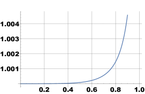
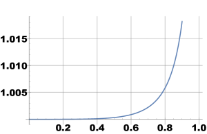
Figure 1. 1: The graph of $\mu(r)/u_{1}(r)$, where $0<r<1$ 1: The graph of $v_{2}(r)/\mu(r)$, where $0<r<1$.

Remark 2.13.

It is worth mentioning that the new upper and lower bounds for $\varphi_{K}$ are more accurate than those bounds in (2.15). Indeed,

$$r^{1/K}<u_{1}^{-1}(u_{1}(r)/K)<\varphi_{K}(r)<v_{2}^{-1}(v_{2}(r)/K)<4^{1-1/K}r^{1/K}$$

for all $K>1$ and $r\in(0,1)$.

3. Landen Approximations

The three functions $\mu,\mu^{-1},\varphi_{K}$ were extensively investigated in [4], with computer implementations in languages, Mathematica, MATLAB, C on the accompanying diskette. Here our goal is to show that for a large range of the arguments we obtain results with accuracy to those in [4], now only using Mathematica. The methods applied in [4] for the numerical evaluation of  K and $\mu$ were based on the arithmetic-geometric meanwhile for $\mu^{-1}$ and $\varphi_{K}$ a Newton iteration was used. Here we show that the Landen sequences yield approximations with errors close to machine epsilon agreement with the results of [4] when the recursion level is moderate, 4 or 5.

Our starting point is the following lemma.

Lemma 3.1.

(1) The function $\mu(r)+\log r$ is a monotone decreasing function from $(0,1)$ onto $(0,\log 4).$

(2) For $0<r<1,p\in\mathbb{Z}$

$$2^{-p}\log\frac{1}{L(r,-p)}<\mu(r)<2^{-p}\log\frac{4}{L(r,-p)},$$

and, in particular, for $p=1$ we have

$$u_{5}(r)<\mu(r)<v_{2}(r),$$

where $u_{5}$ and $v_{2}$ are defined as in Tables 2 and 3, respectively.

Proof.

(1) This is well-known, see [4, p. 84, Thm 5.13].

(2) The proof follows from (2.13) and part (1). ∎

The upper bound of Lemma 3.1(2) with $p=4$ seems to be very precise. Figure 2 shows the difference $\mu(r)-2^{-4}\log(4/L(r,-4))$, where $r\in(0,1)$ and $\mu(r)$ is computed using the cip.nb file from [4].

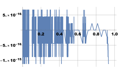
Figure 2. The difference between $\mu(r)$ and the upper bound of Lemma 3.1(2) with $p=4$ and $r\in(0,1)$.

Proposition 3.2.

Let $u,v:(0,1)\rightarrow(0,\infty)$ be continuous functions with $|u(r)-v(r)|<M$ for some constant $M$ and for all $r\in(0,1)$. Also let $u(r)<\mu(r)<v(r)$ for all $r\in(0,1)$. Then

$$\lim_{p\rightarrow-\infty}2^{p}u(L(r,p))=\lim_{p\rightarrow-\infty}2^{p}v(L(r,p))=\mu(r).$$

Proof.

By (2.13)

$$2^{p}u(L(r,p))<\mu(r)=2^{p}\mu(L(r,p))<2^{p}v(L(r,p))$$

which implies that

$$|2^{p}v(L(r,p))-2^{p}u(L(r,p))|<2^{p}M,$$

concluding the proof. ∎

Remark 3.3.

By (2.18) we can apply Proposition 3.2, for example, with $u_{2}$ and $v_{2}$, where $u_{2}$ and $v_{2}$ are defined as in Tables 2 and 3, respectively.

Below, we will find the best and simplest approximation for $\mu^{-1}(y)$, based on the Landen transformation.

Proposition 3.4.

Let $u,v:(0,1)\rightarrow(0,\infty)$ be decreasing homeomorphism with $u(r)<\mu(r)<v(r)$ for all $r\in(0,1)$. Then for $y>0$ and $r=\mu^{-1}(y)$ we have

$$L(u^{-1}(2^{-p}y),-p)<r=\mu^{-1}(y)<L(v^{-1}(2^{-p}y),-p).$$

Proof.

By (2.13)

$$y=\mu(r)=2^{p}\mu(L(r,p))<2^{p}v(L(r,p))$$

and because $v$ is decreasing $L(r,p)<v^{-1}(2^{-p}y)$. Hence $r<L(v^{-1}(2^{-p}y),-p)$. The proof of the lower bound is similar, so we omit the details. ∎

Remark 3.5.

We know by (2.19) that

$$u_{1}(r)<\mu(r)<v_{1}(r)$$

for all $r\in(0,1)$, where $u_{1}$ and $v_{1}$ are defined as in Tables 2 and 3, respectively. It is easy to see that $u_{1}$ and $v_{1}$ are a homeomorphism of $(0,1)$ onto $(0,\infty)$. Applying Proposition 3.4 with $u_{1}(r)$, $v_{1}(r)$, and their inverses we obtain

$$\mu^{-1}(y)\approx L\left(u_{1}^{-1}(2^{-p}y),-p\right)=:f_{1}(y,p)$$

and

$$\mu^{-1}(y)\approx L\left(v_{1}^{-1}(2^{-p}y),-p\right)=:g_{1}(y,p).$$

It also follows from (2.18) that the following inequalities

$$u_{3}(r)<\mu(r)<v_{2}(r),$$

hold true for $r\in(0,1)$, where $u_{3}$ and $v_{2}$ are a homeomorphism of $(0,1)$ onto $(0,\infty)$ and $(\log 2,\infty)$, respectively. If we apply Proposition 3.4 for $u_{3}$ and $v_{2}$, we get

$$\mu^{-1}(y)\approx L\left(u_{3}^{-1}(2^{-p}y),-p\right)=:f_{2}(y,p)$$

and

$$\mu^{-1}(y)\approx L\left(v_{2}^{-1}(2^{-p}y),-p\right)=:g_{2}(y,p).$$

Finally, applying

$$u_{4}(r)<\mu(r)<v_{3}(r)$$

and applying Proposition 3.4 with $u_{4}$ and $v_{3}$ (which are a homeomorphism of $(0,1)$ onto $(0,\infty)$ and $(\log 4,\infty)$, respectively) we obtain

$$\mu^{-1}(y)\approx L\left(u_{4}^{-1}(2^{-p}y),-p\right)=:f_{3}(y,p)$$

and

$$\mu^{-1}(y)\approx L\left(v_{3}^{-1}(2^{-p}y),-p\right)=:g_{3}(y,p).$$

Computational results for some values $y$ in the range $(0.2,20)$ are summarized in Table 5. Only the cases $p=-4,-5$ are taken into account in this table. When $p=\ldots,-6,-3,-2,-1,\ldots$ the error is large.

$y$	$\mu^{-1}(y)-g_{2}(y,-4)$	$\mu^{-1}(y)-g_{3}(y,-5)$
$0.5$	$0$	$0$
$1.5$	$-2.22045\times 10^{-16}$	$-2.22045\times 10^{-16}$
$2.5$	$1.11022\times 10^{-16}$	$1.11022\times 10^{-16}$
$3.5$	$-1.38778\times 10^{-17}$	$-1.38778\times 10^{-17}$
$4.5$	$2.08167\times 10^{-17}$	$2.08167\times 10^{-17}$
$5.5$	$0$	$0$
$6.5$	$0$	$0$
$7.5$	$-1.30104\times 10^{-18}$	$-1.30104\times 10^{-18}$
$8.5$	$-4.33681\times 10^{-19}$	$-4.33681\times 10^{-19}$
$9.5$	$-7.58942\times 10^{-19}$	$-7.58942\times 10^{-19}$
$10.5$	$-2.1684\times 10^{-19}$	$-2.1684\times 10^{-19}$
$11.5$	$3.38813\times 10^{-20}$	$3.38813\times 10^{-20}$
$12.5$	$-1.18585\times 10^{-20}$	$-1.18585\times 10^{-20}$
$13.5$	$-3.38813\times 10^{-21}$	$-3.38813\times 10^{-21}$
$14.5$	$-4.23516\times 10^{-22}$	$0$
$15.5$	$-1.90582\times 10^{-21}$	$-1.90582\times 10^{-21}$
$16.5$	$-5.82335\times 10^{-22}$	$-5.82335\times 10^{-22}$
$17.5$	$2.24993\times 10^{-22}$	$2.24993\times 10^{-22}$
$18.5$	$7.27919\times 10^{-23}$	$7.27919\times 10^{-23}$
$19.5$	$1.65436\times 10^{-23}$	$1.65436\times 10^{-23}$

Table 5. The error between $\mu^{-1}(y)$ and $g_{2}(y,-4)$, and $\mu^{-1}(y)$ and $g_{3}(y,-5)$ for some values in range $y\in(0.2,20)$. For the computation of $\mu^{-1}(y)$ we have used the Mathematica "cip.m" file from [4, Appendix B].

Computer experiments show that $g_{2}(y,-4)$ and $g_{3}(y,-5)$ are the best approximations for $\mu^{-1}(y)$. We note that $\mu^{-1}(y)-g_{2}(y,-4)$ and $\mu^{-1}(y)-g_{3}(y,-5)$ have an error value of order $10^{-14},\ldots,10^{-24}$ in the interval $(0.2,20)$, see Figure 3. For the computation of $\mu^{-1}(y)$ we use the Mathematica "cip.m" file from [4, Appendix B].

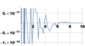
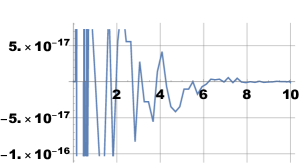
Figure 3. 1: The graph of $\mu^{-1}(y)-g_{2}(y,-4)$, where $0<y<10$ 1: The graph of $\mu^{-1}(y)-g_{3}(y,-5)$, where $0<y<10$.

$p$	$\mu^{-1}(y)$	$\mu(r)$
$1$	$\displaystyle{\frac{4\sqrt{\exp(-\max\{2r,\log 4\})}}{1+4\exp(-\max\{2r,\log 4\})}}$	$\displaystyle{\log\frac{2(1+r^{\prime})}{r}}$
$2$	$\displaystyle{\frac{4\sqrt{\frac{\sqrt{\exp(-\max\{4r,\log 4\})}}{1+4\exp(-\max\{4r,\log 4\})}}}{1+\frac{4\sqrt{\exp(-\max\{4r,\log 4\})}}{1+4\exp(-\max\{4r,\log 4\})}}}$	$\displaystyle{\frac{1}{4}\log\frac{4\left(1+r^{\prime}\right)^{4}\left(1+\sqrt{w}\right)^{2}}{r^{4}}}$

Table 6. Two steps of Landen approximations of $\mu^{-1}$ by $g_{3}(y,-p))$, and $\mu$ by Lemma 3.1(2).

3.1.

The special function $\varphi_{K}(r)$. In the study of Hölder continuity of quasiconformal mappings of the plane, the special function $\varphi_{K}(r)$ defined as (2.14) has an important role. Based on Proposition 3.2 and Remark 3.5 we study the approximation [4, Theorem 5.43]

(3.2) $$\varphi_{K}(r)=L(\varphi_{K}(L(r,-p)),p)\approx L\left(4^{1-1/K}L(r,-p)^{1/K},p\right)=:L_{\varphi}(K,r,p)$$

for various values of $p$. Table 7 shows a structural formula for $L_{\varphi}(K,r,p)$, where $p=0,1$.

$p$	$L_{\varphi}(K,r,p)$	c
$0$	$4^{1-1/K}r^{1/K}$	$-$
$1$	${\displaystyle{\frac{2\sqrt{4^{1-1/K}\,\,c^{1/K}}}{1+4^{1-1/K}\,\,c^{1/K}}}}$	$\displaystyle{\left(\frac{r}{1+\sqrt{1-r^{2}}}\right)^{2}}$

Table 7. The function $L_{\varphi}(K,r,p)$ for $p=0,1$.

Here we note that $L_{\varphi}(K,r,p)$ is a majorant for the function $\varphi_{K}(r)$. We also study the following approximation by applying Remark 3.5 and Lemma 3.1(2)

(3.3) $$\varphi_{K}(r)\approx g_{3}\left(2^{-p}\log(4/L(r,-p))/K,-5\right)=:LM(K,r,p),$$

where $K>1$, and $r\in(0,1)$. Computer experiments show that $LM(K,r,5)$ is the best approximation for $\varphi_{K}(r)$, see Figure 4.

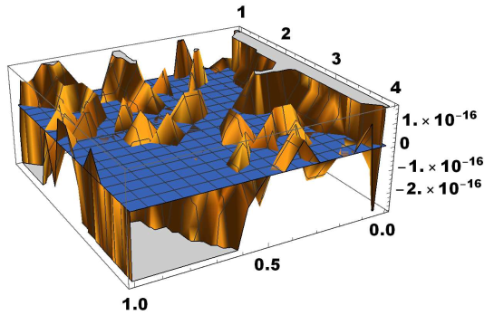
Figure 4. The 3D plot of $\varphi_{K}(r)-LM(K,r,5)$ for $1<K<4$ and $0<r<1$.

3.4.

Remark. The next few lines of Mathematica code

L[s_, p_] :=  Module[{j = 0, y = s},
   While[((j < Abs[p])), If[p < 0, y = (y / (1 + Sqrt[1 - y^2]))^2,
     y = 2 * Sqrt[y] / (1 + y) ]; j++]; y];
LPhi[K_, r_, p_] := L[4 * Exp[(1 / K) * Log[L[r, -p] / 4]], p];

define an approximation for $\varphi_{K}$. This function satisfies

(3.5) $$4^{1-1/K}r^{1/K}>{\tt LPhi[K,r,1]}$$

as we see using the command

 Plot3D[{0, 4^(1 - 1/K) r^(1/K) - LPhi[K, r, 1]}, {r, 0, 1}, {K, 1, 3}]
 

The LHS function of (3.5) here is a majorant for $\varphi_{K},K>1,$ i.e. $\varphi_{K}(r)<4^{1-1/K}r^{1/K}$ for $K>1,r\in(0,1)$ by [8, Thm 9.32].

The RHS function LPhi[K, r, 1] of (3.5) is not a majorant for $\varphi_{K},K>1,$ because for the values $K=2,r=0.9$ it is smaller than $\varphi_{2}(r)=2\sqrt{r}/(1+r),$ that is $\varphi_{2}(0.9)=0.998614>0.993649={\tt LPhi[2,0.9,1]}$.

3.6.

Conclusion. For $K\in(1,20)$ and $r\in(0,1)$ the approximations (3.2) and (3.3) with $p=5$ yield maximal error of the order $10^{-14}$. The reported error is based on the identity (2.17). The approximation (3.2) based only on the Landen transformation is remarkably simple and precise, as it makes no use of elliptic integrals. One could also use this identity (2.16) to test the above algorithm.

3.7.

Some open problems. Computational experiments have led us to formulate the following questions:
(1) Let $L_{\varphi}(K,r,p)$ be defined as in (3.2). Then

$$L_{\varphi}(K,r,p)\leq 4^{1-{1}/{K}}r^{{1}/{K}}$$

for $1<K<4.6$, $r\in(0,0.7]$, and $p=0,1,2,\ldots$.

Motivation. Considering that $p=0$ is obvious, we may assume that $p=1,2,3,\ldots$. Since $L(\cdot,p):(0,1)\rightarrow(0,1)$ is an increasing homeomorphism, we are looking for $r\in(0,1)$ and $K>1$ such that $4^{1-1/K}L(r,-p)^{1/K}<1$. Computer experiments show that $4^{1-1/K}L(r,-p)^{1/K}<1$ holds true for all $r\in(0,0.7]$, $1<K<4.6$, and $p=1,2,\ldots$.

(2) Remark 3.4 only deals with the case $p=1$. What about $p=2$? Can we find some pair of functions $u,v$ where $u$ is a minorant of $\mu$ and $v$ a majorant of $\mu$ such that the corresponding $L_{\varphi}(K,r,1)$ would be a majorant of $\varphi_{K}$?

Funding
The first author received financial support provided by the Doctoral Programme (formerly MATTI and now EXACTUS) of the Department of Mathematics and Statistics of the University of Turku. The research of the second author was supported by the Finnish Cultural Foundation.

Orcid
Rahim Kargar ORCID ID: http://orcid.org/0000-0003-1029-5386
Oona Rainio ORCID ID: http://orcid.org/0000-0002-7775-7656
Matti Vuorinen ORCID ID: http://orcid.org/0000-0002-1734-8228