Effective Heat Transfer Between a Porous Medium and a Fluid Layer: Homogenization and Simulation

Abstract

We are investigating the effective heat transfer in complex systems involving porous media and surrounding fluid layers in the context of mathematical homogenization. We differentiate between two fundamentally different cases: Case (a), where the solid part of the porous media is assumed to consist of disconnected inclusions and Case (b), where the solid matrix is assumed to be connected. For both scenarios, we consider a heat equation with convection where a small scale parameter $\varepsilon>0$ characterizes the heterogeneity of the porous medium and conduct a limit process $\varepsilon\to 0$ via two-scale convergence for the solutions of the $\varepsilon$-problems. In Case (a), we arrive at a one-temperature problem exhibiting a memory term and, in Case (b), at a two-phase mixture model. We compare and discuss these two limit models with several simulation studies both with and without convection.

Keywords: Homogenization, mathematical modeling, FEniCS simulations, heat transfer, memory terms

MSC2020: 80M40, 35B27, 65N30, 80A19, 76S05

1 Introduction

The effective transfer of (heat) energy at interfaces between fluid-saturated porous media and adjacent fluid layers plays an important role in many applications; drying processes, metalworking with cutting fluids, geothermal engineering, or transpiration cooling to name just a few [3]. The exact conditions usually depend not just on the specific application but also on the precise geometric setup of the porous medium. One specific application motivating our research is the impact of cooling fluids during grinding processes. Some grinding wheels exhibit a porous behaviour due to the binding material while the mechanical forces during grinding processes lead to a substantial heat production. But, as there is a constant resupply of cooling fluid, local thermal equilibrium ([38]) between the fluid inside the porous media and the solid matrix may not hold. In addition, the specific transfer conditions for the heat across the interface between porous media and fluid layer are unclear. Some early experimental investigations and corresponding simulations for such a scenario can be found in [39].

From an engineering, more applied perspective, this search for effective transfer conditions is often conducted via volume averaging techniques [38]. Regarding the specific case of effective heat transfer conditions, the seminal work of Ochoa-Tapia and Whitaker [30], where flux conditions were formally derived under the assumption of continuity of temperature and velocity across the interface, stands out; though, as is often the case, there were some earlier contributions as well, e.g., [33, 34, 37]. With similar approaches several different models and conditions were derived and discussed based on that, cf. [1, 4, 24, 29, 40]. However, there still seems to be some disagreement about under which circumstances those models are valid [29].

A different strategy is usually chosen in the context of mathematical homogenization, where limits are investigated with respect to a scale parameter $\varepsilon$. Two-temperature models describing the dispersive and convective transport in porous media were derived in [20]. Closely related, thermo-elasticity problems for different two-phase structures were investigated in [13, 15]. To our knowledge, there does not yet exist a rigorous investigation of the effective heat transfer model for porous media in contact with a fluid layer. Similar geometric setups can be found in fluid scenarios (without heat) involving an interface between porous media and fluid layers, e.g., [14, 25, 27].

In this work, we start with a two-domain heat-equation for the fluid and solid phase of our system with imperfect heat transfer and a prescribed fluid velocity. Conducting a limit analysis with respect to a scale parameter $\varepsilon$ representing the size of the microstructures of the porous media, we identify effective model descriptions. This is done for two different sets of microstructures (see also Fig. 1):

• Case (a): Disconnected solid inclusions inside the fluid. Here, we arrive at a two-scale problem where the solid takes the role of distributed microstructures similarly as in [12, 35] (Theorem 2). We show that the solid temperature can be eliminated from this model via a memory term, leading to a non-local in time parabolic limit system (lemma 1). For examples with comparable memory terms in the context of porous media we point to [2, 5, 9, 11, 32].

• Case (b): Both the pore space and the solid matrix are connected. Here, the limit problem is structurally a two-phase mixture model similar to [19, 40] (Theorem 3).

Numerical investigations for similar limit problems can be found in the literature, e.g., [1, 3, 33]. In our finite element simulations (using FEniCS), we experiment with different parameters (e.g., heat conductivity, permeability) to compare the two different models both with and without convection. In particular, we are able to highlight the transition from Case (b) to Case (a) for geometries with bad connectivity (see Section 5.1).

This paper is structured as follows: In Section 2, we introduce the mathematical model and the two different geometric setups. This is followed by Section 3, where we present the main results, in particular the homogenization limits for the disconnected case (Theorem 2) and the connected case (Theorem 3). The detailed proof of these limits via two-scale convergence is presented in Section 4. Finally, in Section 5, several simulation results are used to compare the different homogenization limits in cases with and without convection.

2 Setup, mathematical model, and assumptions

In this section, we provide the two different geometric setups as well as the mathematical model we are considering in this work. We also collect the assumptions on the coefficients and data.

First, let $S=(0,T)$, $T>0$, represent the time interval of interest. For some $H>0$, let $\Omega=\tilde{\Omega}\times(0,H)\subset\mathbb{R}^{d}$ ($d=2,3$) where $\tilde{\Omega}\subset\mathbb{R}^{d-1}$ is a bounded Lipschitz domain. For technical reasons, we assume that $\tilde{\Omega}$ is a finite union of axis-parallel cubes with corner coordinates in $\mathbb{Z}^{d-1}$. We denote the outer normal vector of $\Omega$ by $\nu=\nu(x)$. We subdivide $\Omega$ into subdomains $\Omega^{p}=\tilde{\Omega}\times(0,h)$ and $\Omega^{ff}=\tilde{\Omega}\times(h,H)$ (for some $0<h<H$) representing the porous domain and the domain of free-flowing fluid. The interface between these subdomains will be denoted by $\Sigma=\tilde{\Omega}\times\{h\}$.

Now, for the reference geometry, let $Y=(0,1)^{d}$. Take $Y^{f},$ $Y^{s}\subset Y$ to be two disjointed Lipschitz domains such that $Y=Y^{f}\cup Y^{s}\cup\Gamma$ where $\Gamma:=\overline{Y^{f}}\cap\overline{Y^{s}}$. Also, let $\Sigma_{0}=(0,1)^{d-1}\times\{0\}$ denote the lower face of the unit cube. Let $\varepsilon_{0}>0$ be chosen such that $\Omega$ can be perfectly tiled with $\varepsilon_{0}Y$ cells and set $\varepsilon_{n}=2^{-n}\varepsilon_{0}$. We introduce the periodic structures (for the sake of readability we suppress the subscript $n$ and just write $\varepsilon$)

$$Z_{\varepsilon}^{r}=\operatorname{int}\left(\bigcup_{k\in\mathbb{Z}^{d}}\varepsilon(\overline{Y^{r}}+k)\right)\quad(r=s,f)$$

and consider two distinct specific cases:

• Case (a): We assume $\overline{Y^{s}}\subset Y$. As a consequence, $Z_{\varepsilon}^{s}$ is disconnected.

• Case (b): $Z_{\varepsilon}^{r}$ are Lipschitz domains for both phases $r=f,s$. In particular, both sets are connected.

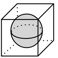
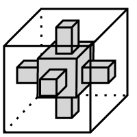
Figure 1: Left: two dimensional cross-section of the macroscopic domain $\Omega$. Middle: unit cell representing the disconnected solid inclusions. Right: unit cell representing a connected solid matrix.

In both cases, the normal vector of $\Gamma$ pointing outwards of $Y^{s}$ will be denoted with $n_{\Gamma}=n_{\Gamma}(y)$, $y\in\Gamma$. Now, for $\varepsilon>0$, we introduce the $\varepsilon Y$-periodic domains $\Omega_{\varepsilon}^{f}$, $\Omega_{\varepsilon}^{s}\subset\Omega^{p}$ and the interface $\Gamma_{\varepsilon}$ representing the fluid and solid parts of the porous domain and their internal boundary, respectively:

$$\Omega_{\varepsilon}^{f}=\operatorname{int}\left(\overline{\Omega^{ff}}\cup\left(\Omega^{p}\cap Z_{\varepsilon}^{f}\right)\right),\quad\Omega_{\varepsilon}^{s}=\Omega^{p}\cap Z_{\varepsilon}^{s},\quad\Gamma_{\varepsilon}=\Omega^{p}\cap\left(\bigcup_{k\in\mathbb{Z}^{d}}\varepsilon(\overline{\Gamma}+k)\right).$$

In Case (a) $\Omega_{\varepsilon}^{f}$ is connected and $\Omega_{\varepsilon}^{s}$ is disconnected; in Case (b) both phases are connected. The normal vector of $\Gamma_{\varepsilon}$ pointing outwards $\Omega_{\varepsilon}^{s}$ is given by $n_{\varepsilon}=n_{\varepsilon}(x)$, $x\in\Gamma_{\varepsilon}$. We also introduce the sets

$$\Sigma_{\varepsilon}^{r}=\overline{\Omega_{\varepsilon}^{r}}\cap\Sigma,\quad(\partial\Omega)_{\varepsilon}^{r}=\partial\Omega_{\varepsilon}^{p}\cap\partial\Omega$$

and note that in Case (a) $\Sigma_{\varepsilon}^{s}=(\partial\Omega)_{\varepsilon}^{s}=\emptyset$. In the following, $\chi_{\varepsilon}^{r}\colon\Omega\to\{0,1\}$ and $\chi^{r}\colon Y\to\{0,1\}$ denotes the characteristic functions corresponding to $\Omega_{\varepsilon}^{i}$ and $Y^{r}$, respectively.

Now, regarding the mathematical model, let $\theta_{\varepsilon}^{r}=\theta_{\varepsilon}^{r}(t,x)$ ($r=f,s$) represent the temperature at time $t\in S$ at $x\in\Omega_{\varepsilon}^{r}$. The standard linear heat equation models the heat dynamics in fluid and solid regions via

$$\rho^{f}c^{f}\partial_{t}\theta_{\varepsilon}^{f}-\operatorname{div}(\kappa^{f}\nabla\theta_{\varepsilon}^{f}-\rho^{f}c^{f}v_{\varepsilon}\theta_{\varepsilon}^{f}) =f_{\varepsilon}^{f} \text{in}\ \ S\times\Omega_{\varepsilon}^{f},$$ (1a)

$$\rho^{s}c^{s}\partial_{t}\theta_{\varepsilon}^{s}-\operatorname{div}(\kappa^{s}_{\varepsilon}\nabla\theta_{\varepsilon}^{s}) =f_{\varepsilon}^{s} \text{in}\ \ S\times\Omega_{\varepsilon}^{s}.$$ (1b)

Here, $$\rho^{r} r c^{r} \kappa^{f} \kappa_{\varepsilon}^{s} f_{\varepsilon}^{r} v_{\varepsilon} v_{\varepsilon}\cdot n_{\varepsilon}=0 \Gamma_{\varepsilon}$$ denotes the mass density of phase , the specific heat, , the heat conductivities, and possible volume source densities. Moreover, denotes the Eulerian fluid velocity that is assumed to be given a priori (see also Remark 1) but has to satisfy on , i.e., no inflow of fluid into the solid structure is possible.

Remark 1.

In a general setting, the velocity $v_{\varepsilon}$ should ideally be given via the solution to a Navier-Stokes or Stokes system. In our setting, we just assume the velocity to be given and to satisfy certain assumptions that we specify later.

At the fluid-solid interface $\Gamma_{\varepsilon}$, we assume continuity of fluxes (energy balance) and heat exchange via temperature difference (here, we use $v_{\varepsilon}\cdot n_{\varepsilon}=0$)

$$-\kappa^{f}\nabla\theta_{\varepsilon}^{f}\cdot n_{\varepsilon} =-\kappa_{\varepsilon}^{s}\nabla\theta_{\varepsilon}^{s}\cdot n_{\varepsilon} \text{on}\ \ S\times\Gamma_{\varepsilon},$$ (1c)

$$\kappa^{f}\nabla\theta_{\varepsilon}^{f}\cdot n_{\varepsilon} =\alpha_{\varepsilon}(\theta_{\varepsilon}^{f}-\theta_{\varepsilon}^{s}) \text{on}\ \ S\times\Gamma_{\varepsilon}.$$ (1d)

Here, $\alpha_{\varepsilon}$ denotes the heat exchange coefficient. Finally, we pose homogeneous Neumann boundary condition at the outer boundary and initial conditions ($r=f,s$):

$$-\kappa^{r}\nabla\theta_{\varepsilon}^{r}\cdot\nu =0 \text{on}\ \ S\times(\partial\Omega)_{\varepsilon}^{r},$$ (1e)

$$\theta_{\varepsilon}^{r} =\theta_{\varepsilon,0}^{r} \text{in}\ \ \Omega_{\varepsilon}^{r}.$$ (1f)

Please note that in Case (a), condition (1e) is vacuously true for the solid part as $(\partial\Omega)_{\varepsilon}^{s}=\emptyset$ and $(\partial\Omega)_{\varepsilon}^{f}=\partial\Omega$, but in Case (b) both conditions are needed. The $\varepsilon$-dependent micro-model in its PDE form is then given by System (1).

In the following, we collect the main assumptions we are placing on the coefficients and data regarding the problem. The precise definition of a solution will be presented in Section 3. In general, for a function $f$ defined on $\Omega_{\varepsilon}^{f}$ or $\Omega_{\varepsilon}^{s}$, $\tilde{f}$ denotes the trivial zero-continuation to the whole of $\Omega$ or $\Omega^{p}$, respectively. Also, the subscript $\#$ in function spaces is taken to indicate periodicity, e.g.,

$$H^{1}_{\#}(Y):=\left\{u\in H^{1}_{loc}(\mathbb{R}^{d})\ :\ u_{|Y}\in H^{1}(Y),\ \ u(x+e_{i})=u(x)\ \text{for almost all}\ x\in\mathbb{R}^{d},\ i=1,2,3\right\}.$$

Assumptions on the data.

• The coefficients $\rho^{r}$, $c^{r}$, and $\kappa^{f}$ are positive. Also, there are positive constants $\alpha$, $\kappa^{s}$ such that

  • $\Omega_{\varepsilon}^{s}$ disconnected: $\kappa_{\varepsilon}^{s}=\varepsilon^{2}\kappa^{s}$, $\alpha_{\varepsilon}=\varepsilon\alpha$

  • $\Omega_{\varepsilon}^{s}$ connected: $\kappa_{\varepsilon}^{s}=\kappa^{s}$, $\alpha_{\varepsilon}=\varepsilon\alpha\chi_{\Gamma_{\varepsilon}\cap\Omega^{p}}+\alpha\chi_{\Sigma_{\varepsilon}^{s}}$

  Please note that the $\varepsilon^{2}$-scaling in Case (a) is standard for this particular typ of the disconnected solid geometry, cf. [7, 11, 16, 23] for comparable situations. The heat exchange coefficient $\alpha$ is scaled with $\varepsilon$ to counteract the interface blow-up $\varepsilon|\Gamma_{\varepsilon}|=|\Omega^{p}||\Gamma|$; as is common with this kind of interface terms [23, 28, 31]. In the connected case, the additional interface $\Sigma_{\varepsilon}^{s}$ does not blow-up and for that reason is not scaled.

• The volume source densities $(f_{\varepsilon}^{f},f_{\varepsilon}^{s})\in L^{2}(S\times\Omega_{\varepsilon}^{f})\times L^{2}(S\times\Omega_{\varepsilon}^{s})$ satisfy

  $$C_{f}:=\sup_{\varepsilon>0}\left(\|f_{\varepsilon}^{f}\|_{L^{2}(S\times\Omega_{\varepsilon}^{f})}^{2}+\|f_{\varepsilon}^{s}\|^{2}_{L^{2}(S\times\Omega_{\varepsilon}^{s})}\right)<\infty.$$

• The initial conditions $(\theta_{\varepsilon,0}^{f},\theta_{\varepsilon,0}^{s})\in L^{2}(\Omega_{\varepsilon}^{f})\times L^{2}(\Omega_{\varepsilon}^{s})$ satisfy

  $$C_{0}:=\sup_{\varepsilon>0}\left(\|\theta_{\varepsilon,0}^{f}\|_{L^{2}(\Omega_{\varepsilon}^{f})}^{2}+\|\theta_{\varepsilon,0}^{s}\|^{2}_{L^{2}(\Omega_{\varepsilon}^{s})}\right)<\infty.$$

• The velocity $v_{\varepsilon}\in L^{\infty}(S\times\Omega_{\varepsilon}^{f})^{d}$ satisfies

  $$C_{v}:=\sup_{\varepsilon>0}\|v_{\varepsilon}\|_{L^{\infty}(S\times\Omega_{\varepsilon}^{f})}<\infty.$$

  Also, we assume the fluid to be incompressible as well as $v_{\varepsilon}\cdot n_{\varepsilon}=0$ on $\Gamma_{\varepsilon}$.

• There are limit functions $f^{f}\in L^{2}(S\times\Omega)$ as well as $\theta_{0}^{f}\in L^{2}(S\times\Omega)$ such that

  $$\tilde{f}_{\varepsilon}^{f}\to f^{f},\quad\tilde{\theta}_{\varepsilon}^{f}\to\theta_{0}^{f}\quad\text{in}\ L^{2}(S\times\Omega).$$

• • $\Omega_{\varepsilon}^{s}$ disconnected. There are functions $f^{s}\in L^{2}(S\times\Omega^{p}\times Y)$ as well as $\theta_{0}^{s}\in L^{2}(\Omega^{p}\times Y)$ such that

    $$f_{\varepsilon}^{s}\stackrel{{\scriptstyle 2}}{{\rightharpoonup}}\chi^{s}f^{s},\quad\theta_{\varepsilon,0}^{s}\stackrel{{\scriptstyle 2}}{{\rightharpoonup}}\chi^{s}\theta_{0}^{s}.$$

  • $\Omega_{\varepsilon}^{s}$ connected. There are functions $f^{s}\in L^{2}(S\times\Omega^{p})$ as well as $\theta_{0}^{s}\in L^{2}(\Omega^{p})$ such that

    $$f_{\varepsilon}^{s}\to f^{s},\quad\theta_{\varepsilon,0}^{s}\to\theta_{0}^{s}\quad\text{in}\ L^{2}(S\times\Omega).$$

• There are functions $v\in L^{2}(S\times\Omega^{ff})$, $v_{D}\in L^{2}(S\times\Omega^{p};H_{\#}^{1}(Y))$ where $v_{D}(t,\cdot,y)\in H^{1}(\Omega^{p})$ for almost all $(t,y)\in S\times Y$ such that

  $$v_{\varepsilon}\to v\quad\text{in}\ L^{2}(S\times\Omega^{ff}),\quad{\tilde{v}_{\varepsilon}}{}_{|\Omega^{p}}\stackrel{{\scriptstyle 2}}{{\rightharpoonup}}\chi^{f}v_{D}.$$

  We also assume that $v_{D}\cdot n_{\Gamma}=0$ almost everywhere on $S\times\Omega\times\Gamma$ and incompressibility, i.e., $\operatorname{div}_{y}v_{D}=0$ almost everywhere in $S\times\Omega\times Y^{f}$.

From this list, Assumptions (A1)-(A4) are needed to ensure the existence of unique solutions with certain $\varepsilon$-uniform estimates and Assumptions (A5)-(A7) for the limit process $\varepsilon\to 0$. The letters (a) and (b) indicate the specific geometric setup.

Remark 2.

Relating to Remark 1, in a more general setting, we would hope to find the limit functions $v$ and $v_{D}$ via a limit process done on an $\varepsilon$-dependent Stokes problem for the initial fluid-solid system. These kinds of problems were investigated in. e.g., [14, 25] and lead to specific interface conditions (like Joseph-Beavers-Saffmann) at $\Sigma$ that allow for velocity discontinuities laterally to the interface. The limit function $v_{D}$, in that example, would be the well-known Darcy velocity. This, Stokes flow for $\Omega^{ff}$ coupled with Darcy flow in $\Omega^{p}$ with Joseph-Beavers condition is also the approach taken in the simulations (see section 5.2).

3 Main results

We fix our solution space

$$W_{\varepsilon}=\left\{(u^{f},u^{s})\in L^{2}(S;H^{1}(\Omega_{\varepsilon}^{f})\times H^{1}(\Omega_{\varepsilon}^{s}))\ :\ \partial_{t}(u^{f},u^{s})\in L^{2}(S;L^{2}(\Omega_{\varepsilon}^{f}\times\Omega_{\varepsilon}^{s}))\right\}$$

and call $(\theta_{\varepsilon}^{f},\theta_{\varepsilon}^{s})\in W_{\varepsilon}$ a solution to the $\varepsilon$-dependent problem given by System (1) if it satisfies $(\theta_{\varepsilon}^{f}(0),\theta_{\varepsilon}^{s}(0))=(\theta_{\varepsilon,0}^{f},\theta_{\varepsilon,0}^{s})$ as well as

$$(\rho^{f}c^{f}\partial_{t}\theta_{\varepsilon}^{f},\varphi^{f})_{\Omega_{\varepsilon}^{f}}+(\kappa^{f}\nabla\theta^{f}_{\varepsilon}-\rho^{f}c^{f}v_{\varepsilon}\theta^{f}_{\varepsilon},\nabla\varphi^{f})_{\Omega_{\varepsilon}^{f}}+(\rho^{s}c^{s}\partial_{t}\theta_{\varepsilon}^{s},\varphi^{s})_{\Omega_{\varepsilon}^{s}}+\kappa_{\varepsilon}^{s}(\nabla\theta^{s}_{\varepsilon},\nabla\varphi^{s})_{\Omega_{\varepsilon}^{s}}\\ +\alpha_{\varepsilon}(\theta_{\varepsilon}^{f}-\theta_{\varepsilon}^{s},\varphi^{f}-\varphi^{s})_{\Gamma_{\varepsilon}}=(f_{\varepsilon}^{f},\varphi^{f})_{\Omega_{\varepsilon}^{f}}+(f_{\varepsilon}^{s},\varphi^{s})_{\Omega_{\varepsilon}^{s}}$$ (2)

for all test functions $(\varphi^{f},\varphi^{s})\in H^{1}(\Omega_{\varepsilon}^{f})\times H^{1}(\Omega_{\varepsilon}^{s})$ and almost all $t\in S$.

Theorem 1 (Existence and estimates).

Let Assumptions (A1)-(A4) be satisfied. Then, there is a unique $(\theta_{\varepsilon}^{f},\theta_{\varepsilon}^{s})\in W_{\varepsilon}$ satisfying $(\theta_{\varepsilon}^{f}(0),\theta_{\varepsilon}^{s}(0))=(\theta_{\varepsilon,0}^{f},\theta_{\varepsilon,0}^{s})$ and (2) for all test functions $(\varphi^{f},\varphi^{s})\in H^{1}(\Omega_{\varepsilon}^{f})\times H^{1}(\Omega_{\varepsilon}^{s})$ and almost all $t\in S$. In addition, it holds

$$\|\theta_{\varepsilon}^{f}\|^{2}_{L^{\infty}(S;L^{2}(\Omega_{\varepsilon}^{f}))}+\|\theta_{\varepsilon}^{s}\|^{2}_{L^{\infty}(S;L^{2}(\Omega_{\varepsilon}^{s}))}+\|\nabla\theta_{\varepsilon}^{f}\|^{2}_{L^{2}(S\times\Omega_{\varepsilon}^{f})}+\varepsilon^{\gamma}\|\nabla\theta_{\varepsilon}^{s}\|^{2}_{L^{2}(S\times\Omega_{\varepsilon}^{s})}+\varepsilon\|\theta_{\varepsilon}^{f}-\theta_{\varepsilon}^{s}\|^{2}_{L^{2}(S\times\Gamma_{\varepsilon})}\leq C$$ (3)

where $\gamma=2$ in Case (a) and $\gamma=0$ in Case (b).

Proof.

For each $\varepsilon>0$, equation (2) is the weak form of a standard advection-diffusion parabolic system that admits a unique solution $(\theta_{\varepsilon}^{f},\theta_{\varepsilon}^{s})\in W_{\varepsilon}$ under the given assumptions. The estimates are the result of energy estimates: Taking $(\theta_{\varepsilon}^{f},\theta_{\varepsilon}^{s})$ as a test function, we get

$$\rho^{f}c^{f}\frac{\operatorname{d}}{\operatorname{d}t}\|\theta_{\varepsilon}^{f}\|^{2}_{L^{2}(\Omega_{\varepsilon}^{f})}+\kappa^{f}\|\nabla\theta^{f}_{\varepsilon}\|^{2}_{L^{2}(\Omega_{\varepsilon}^{f})}+\rho^{s}c^{s}\frac{\operatorname{d}}{\operatorname{d}t}\|\theta_{\varepsilon}^{s}\|^{2}_{L^{2}(\Omega_{\varepsilon}^{s})}+\varepsilon^{\gamma}\kappa^{s}\|\nabla\theta^{s}_{\varepsilon}\|^{2}_{L^{2}(\Omega_{\varepsilon}^{s})}+\varepsilon\alpha\|\theta_{\varepsilon}^{f}-\theta_{\varepsilon}^{s}\|^{2}_{L^{2}(\Gamma_{\varepsilon})}\\ \leq(f_{\varepsilon}^{f},\theta_{\varepsilon}^{f})_{\Omega_{\varepsilon}^{f}}+(f_{\varepsilon}^{s},\theta_{\varepsilon}^{s})_{\Omega_{\varepsilon}^{s}}+\rho^{f}c^{f}(v_{\varepsilon}\theta^{f}_{\varepsilon},\nabla\theta_{\varepsilon}^{f})_{\Omega_{\varepsilon}^{f}}$$

Integrating over $(0,t)$ and using $|v_{\varepsilon}|\leq C_{v}$ (Assumption (A4)) yields

$$\rho^{f}c^{f}\|\theta_{\varepsilon}^{f}(t)\|^{2}_{L^{2}(\Omega_{\varepsilon}^{f})}+\rho^{s}c^{s}\|\theta_{\varepsilon}^{s}(t)\|^{2}_{L^{2}(\Omega_{\varepsilon}^{s})}\\ +\frac{\kappa^{f}}{2}\int_{0}^{t}\|\nabla\theta^{f}_{\varepsilon}\|^{2}_{L^{2}(\Omega_{\varepsilon}^{f})}\,\mathrm{d}\tau+\varepsilon^{r}\kappa^{s}\int_{0}^{t}\|\nabla\theta^{s}_{\varepsilon}\|^{2}_{L^{2}(\Omega_{\varepsilon}^{s})}\,\mathrm{d}\tau+\varepsilon\alpha\int_{0}^{t}\|\theta_{\varepsilon}^{f}-\theta_{\varepsilon}^{s}\|^{2}_{L^{2}(\Gamma_{\varepsilon})}\,\mathrm{d}\tau\\ \leq\int_{0}^{t}(f_{\varepsilon}^{f},\theta_{\varepsilon}^{f})_{\Omega_{\varepsilon}^{f}}\,\mathrm{d}\tau+\int_{0}^{t}(f_{\varepsilon}^{s},\theta_{\varepsilon}^{s})_{\Omega_{\varepsilon}^{s}}\,\mathrm{d}\tau+\frac{(C_{v}\rho^{f}c^{f})^{2}}{2\kappa^{f}}\int_{0}^{t}\|\theta^{f}_{\varepsilon}\|^{2}\,\mathrm{d}\tau+\|\theta_{\varepsilon,0}^{f}\|^{2}_{L^{2}(\Omega_{\varepsilon}^{f})}+\|\theta_{\varepsilon,0}^{s}\|^{2}_{L^{2}(\Omega_{\varepsilon}^{s})}.$$

Consequently, using Gronwalls inequality, we arrive at estimate (3) where $C>0$ is independent of $\varepsilon$. ∎

Theorem 2 (Homogenization (Case a)).

Let Assumptions (A1)-(A8) (in their (a)-Variants) be satisfied. Then, $\theta_{\varepsilon}^{f}\to\theta^{f}$ in $L^{2}(S\times\Omega)$ and $\theta_{\varepsilon}^{s}\stackrel{{\scriptstyle 2}}{{\rightharpoonup}}\theta^{s}$ in $L^{2}(S\times\Omega^{p}\times Y^{s})$ for $\varepsilon\to 0$, where

$$(\theta^{f},\theta^{s})\in L^{2}(S;H^{1}(\Omega))\times L^{2}(S\times\Omega;H^{1}(Y^{s}))\ \text{s.t.}\ (\partial_{t}\theta^{f},\partial_{t}\theta^{s})\in L^{2}(S\times\Omega)\times L^{2}(S\times\Omega\times Y^{s}))$$

is the unique solution of the homogenized fluid-heat system

$$\rho^{f}c^{f}\partial_{t}\theta^{f}-\operatorname{div}(\kappa^{f}\nabla\theta^{f}-\rho^{f}c^{f}v\theta^{f}) =f^{f} \text{in}\ \ S\times\Omega^{ff},$$ (4a)

$$|Y^{f}|\rho^{f}c^{f}\partial_{t}\theta^{f}-\operatorname{div}(\kappa_{h}^{f}\nabla\theta^{f}-\rho^{f}c^{f}\bar{v}_{D}\theta^{f})+\alpha\int_{\Gamma}(\theta^{f}-\theta^{s})\,\mathrm{d}\sigma =|Y^{f}|f^{f} \text{in}\ \ S\times\Omega^{p},$$ (4b)

$$-(\kappa^{f}\nabla\theta^{f}-\rho^{f}c^{f}v\theta^{f})\cdot n_{\Sigma}-(\kappa_{h}^{f}\nabla\theta^{f}+\bar{v}_{D}\theta^{f})\cdot n_{\Sigma} =0 \text{on}\ \ S\times\Sigma,$$ (4c)

$$-\kappa^{f}\nabla\theta^{f}\cdot\nu =0 \text{on}\ \ S\times(\partial\Omega\cap\partial\Omega^{ff}),$$ (4d)

$$-\kappa_{h}^{f}\nabla\theta^{f}\cdot\nu =0 \text{on}\ \ S\times(\partial\Omega\cap\partial\Omega^{p}),$$ (4e)

$$\theta^{f} =\theta^{f}_{0} \text{in}\ \ \Omega,$$ (4f)

coupled with the microscale solid-heat problem

$$\rho^{s}c^{s}\partial_{t}\theta^{s}-\kappa^{s}\Delta_{y}\theta^{s} =f^{s} \text{in}\ \ S\times\Omega^{p}\times Y^{s},$$ (4g)

$$-\kappa^{s}\nabla\theta^{s}\cdot n_{\Gamma} =\alpha(\theta^{s}-\theta^{f}) \text{on}\ \ S\times\Omega^{p}\times\Gamma,$$ (4h)

$$\theta^{s} =\theta_{0}^{s} \text{in}\ \ \Omega^{p}\times Y_{s}.$$ (4i)

The velocity field $\bar{v}_{D}$ and the heat conductivity matrix $\kappa_{h}^{f}$ are given by

$$\bar{v}_{D}(t,x)=\int_{Y^{f}}v_{D}(t,x,y)\,\mathrm{d}y,\quad(\kappa_{h}^{f})_{ij}=\frac{\kappa^{f}}{|Y^{f}|}\int_{Y^{f}}(\nabla_{y}\xi_{i}^{f}+e_{i})\cdot e_{j}\,\mathrm{d}y.$$

Here, the $\xi_{i}^{f}\in H^{1}_{\#}(Y^{f})$ ($i=1,2,3$) are the unique, zero-average solution to the cell problems

$$-\Delta_{y}\xi_{i}^{f} =0 \text{in}\ \ Y^{f},$$ (4j)

$$-\nabla_{y}\xi_{i}^{f}\cdot n_{\Gamma} =e_{i}\cdot n_{\Gamma} \text{on}\ \ \Gamma,$$ (4k)

$$y \mapsto\xi_{i}^{f}(y) \text{is $Y$-periodic}.$$ (4l)

Remark 3.

Since $\theta^{f}$ is continuous across $\Sigma$ (due to $\theta^{f}\in H^{1}(\Omega)$), the fluid heat system can also be written as one equation by considering piece-wise constant coefficients like, e.g., $\widetilde{\rho c}=\chi_{\Omega^{ff}}\rho^{f}c^{f}+\chi_{\Omega^{p}}|Y^{f}|\rho^{f}c^{f}$. This leads to

$$\widetilde{\rho c}\partial_{t}\theta^{f}-\operatorname{div}(\tilde{\kappa}\nabla\theta^{f}-\widetilde{\rho cv}\theta)+\widetilde{\alpha}\int_{\Gamma}(\theta^{f}-\theta^{s})\,\mathrm{d}\sigma =\tilde{f^{f}} \text{in}\ \ S\times\Omega^{ff},$$

$$-\widetilde{\kappa}\nabla\theta^{f}\cdot\nu =0 \text{on}\ \ S\times\partial\Omega,$$

$$\theta^{f} =\theta^{f}_{0} \text{in}\ \ \Omega.$$

Proof.

The convergences, up to a subsequence, and the general limiting procedure are presented in detail in Section 4.1. For uniqueness, let $(\theta_{j}^{f},\theta_{j}^{s})$ be two sets of solution, whose differences we denote by $(\overline{\theta}^{f},\overline{\theta}^{s})$. Standard energy estimates for the differences tell us

$$\frac{\operatorname{d}}{\operatorname{d}t}\|\overline{\theta}^{f}\|^{2}_{L^{2}(\Omega)}+\|\nabla\overline{\theta}^{f}\|^{2}_{L^{2}(\Omega)}+|\Gamma|\|\overline{\theta}^{f}\|_{L^{2}(\Omega)}^{2}\\ \leq C\left(\|\widehat{v}\|_{L^{\infty}(S\times\Omega)}\|\nabla\overline{\theta}^{f}\|_{L^{2}(\Omega)}\|\overline{\theta}^{f}\|_{L^{2}(\Omega)}+\|\overline{\theta}^{s}\|_{L^{2}(\Omega^{p}\times\Gamma)}\|\overline{\theta}^{f}\|_{L^{2}(\Omega)}\right)$$

for the fluid temperature and

$$\frac{\operatorname{d}}{\operatorname{d}t}\|\overline{\theta}^{s}\|^{2}_{L^{2}(\Omega^{p}\times Y^{s})}+2\kappa^{s}\|\nabla\overline{\theta}^{s}\|^{2}_{L^{2}(\Omega^{p}\times Y^{s})}+\alpha\|\overline{\theta}^{s}\|_{L^{2}(\Omega^{p}\times\Gamma)}\leq\alpha\sqrt{\Gamma}\|\overline{\theta}^{s}\|_{L^{2}(\Omega^{p}\times\Gamma)}\|\overline{\theta}^{f}\|_{L^{2}(\Omega)}$$

for the solid temperature. With the application of Youngs and Gronwalls inequalities, it follows that $\overline{\theta}^{f}\equiv 0$ and $\overline{\theta}^{s}\equiv 0$ almost everywhere in $S\times\Omega$ and $S\times\Omega\times Y^{s}$, respectively. With the uniqueness it also follows that the whole sequences converge. ∎

This resulting linear problem is a classical example of a coupled two-scale model for the porous part $\Omega^{p}$, where there is an heat exchange between solid and fluid parts via the volume source density $\alpha\int_{\Gamma}(\theta^{f}-\theta^{s})\,\mathrm{d}\sigma$ and the corresponding boundary condition (4h) for $\theta^{s}$. Please note, that energy conservation (outside the volume sources $f^{f}$ and $f^{s}$) still hold since those contributions balance. Also, while $\theta^{f}$ is continuous across $\Sigma$, the heat coefficient $\kappa_{h}$ will not be (see section 5.1). As a consequence, $\theta^{f}$ is expected to exhibit a kink there as can be seen in the simulations.

One possible interpretation of the solid inclusions is as a heat sink or heat source of the porous medium (depending on the prior history of the system): Due to the imperfect heat transfer between fluid and solid parts, there is an expected delay of temperature equilibrium. If the porous system cools or is heated, the solid heat systems delays this process by acting as a heat source or heat storage, respectively.

This idea can be made mathematically explicit by introducing a memory term accounting for the history of the system. In the resulting system the solid heat system is decoupled at the cost of two additional cell problems.

Lemma 1 (Homogenization with memory term).

The System (4a)-(4l) can alternatively be written as (plus initial, boundary, and interface conditions)

$$\rho^{f}c^{f}\partial_{t}\theta^{ff}-\operatorname{div}(\kappa^{f}\nabla\theta^{ff}-\rho^{f}c^{f}v\theta^{ff}) =f^{ff} \text{in}\ \ S\times\Omega^{ff},$$ (5a)

$$\begin{split}\rho^{f}c^{f}|Y^{f}|\partial_{t}\theta^{f}-\operatorname{div}(\kappa_{h}^{f}\nabla\theta^{f}-\rho^{f}c^{f}\bar{v}_{D}\theta^{f})\hskip 99.58464pt&\\ +\alpha|\Gamma|\theta^{f}-\int_{0}^{t}\theta^{f}(\tau)\psi(t-\tau)\,\mathrm{d}\tau&=|Y^{f}|f^{f}+\bar{\eta}\end{split} \text{in}\ \ S\times\Omega^{f},$$ (5b)

where

$$\psi(t)=\int_{\Gamma}\partial_{t}\xi(t,y)\,\mathrm{d}\sigma,\quad\bar{\eta}(t,x)=\int_{\Gamma}\eta(t,x,y)\,\mathrm{d}\sigma+|\Gamma|\theta_{0}^{f}(x).$$

Here, $\xi\in L^{2}(S;H^{1}(Y^{s}))$ with $\partial_{t}\xi\in L^{2}(S\times Y^{s})$ and $\eta\in L^{2}(S\times\Omega^{p};H^{1}(Y^{s}))$ with $\partial_{t}\eta\in L^{2}(S\times\Omega^{p}\times Y^{s})$, are the unique solutions of the cell problems

$$\rho^{s}c^{s}\partial_{t}\xi-\kappa^{s}\Delta_{y}\xi =0 \text{in}\ \ S\times Y^{s},$$

$$-\kappa^{s}\nabla\xi\cdot n_{\Gamma} =\alpha(\xi-1) \text{on}\ \ S\times\Gamma,$$

$$\xi(0) =0 \text{in}\ \ Y^{s}$$

$$\rho^{s}c^{s}\partial_{t}\eta-\kappa^{s}\Delta_{y}\eta =f^{s} \text{in}\ \ S\times Y^{s},$$

$$-\kappa^{s}\nabla\eta\cdot n_{\Gamma} =0 \text{on}\ \ S\times\Gamma,$$

$$\eta(0) =\theta_{0}^{s}-\theta_{0}^{f} \text{in}\ \ Y^{s}$$

Proof.

We take a closer look at the time convolution

$$\vartheta(t,x,y)=\theta_{0}^{f}(x)+\int_{0}^{t}\theta^{f}(\tau,x)\partial_{t}\xi(t-\tau,y)\,\mathrm{d}\tau$$

that naturally satisfies $\vartheta(0,x,y)=\theta_{0}^{f}(x)$ almost everywhere in $\Omega^{p}\times Y^{s}$. For the regularity, we have

$$\vartheta\in L^{2}(S\times\Omega^{p};H^{1}(Y^{s}))\quad\text{such that}\ \partial_{t}\vartheta\in L^{2}(S\times\Omega^{p}\times Y^{s})$$

We calculate for any test function $\phi\in H^{1}(Y^{s})$ using convolution properties:

$$\int_{Y^{s}}\partial_{t}\vartheta(t,x,y)\phi(y)\,\mathrm{d}y =\int_{Y^{s}}\int_{0}^{t}\partial_{t}\theta^{f}(t-\tau,x)\partial_{t}\xi(\tau,y)\phi(y)\,\mathrm{d}\tau\,\mathrm{d}y,$$

$$\int_{Y^{s}}\nabla_{y}\vartheta(t,x,y)\nabla_{y}\phi(y)\,\mathrm{d}y =\int_{Y^{s}}\int_{0}^{t}\partial_{t}\theta^{f}(t-\tau,x)\nabla_{y}\xi(\tau,y)\nabla_{y}\phi(y)\,\mathrm{d}\tau\,\mathrm{d}y,$$

$$\int_{\Gamma}\alpha(\vartheta(t,x,y)-\theta^{f}(t,x))\phi(y)\,\mathrm{d}\sigma =\int_{\Gamma}\alpha\left(\int_{0}^{t}\partial_{t}\theta^{f}(t-\tau,x)\xi(\tau,y)\,\mathrm{d}\tau-(\theta^{f}(t,x)-\theta_{0}^{f}(x))\right)\phi(y)\,\mathrm{d}\sigma,$$

$$=\int_{\Gamma}\int_{0}^{t}\partial_{t}\theta^{f}(t-\tau,x)\alpha\left(\xi(\tau,y)-1\right)\phi(y)\,\mathrm{d}\tau\,\mathrm{d}\sigma.$$

As a consequence, for almost all $x\in\Omega^{p}$, $\vartheta(\cdot,x,\cdot)$ is the unique weak solution of

$$\rho^{s}c^{s}\partial_{t}\vartheta-\kappa^{s}\Delta_{y}\vartheta =0 \text{in}\ \ S\times Y^{s},$$

$$-\kappa^{s}\nabla\vartheta\cdot n_{\Gamma} =\alpha(\vartheta-\theta^{f}) \text{on}\ \ S\times\Gamma,$$

$$\vartheta(0) =\theta_{0}^{f} \text{in}\ \ Y^{s}.$$

Due to the linearity of the model, we can eliminate $\theta^{s}$ with the cell problem solutions $\vartheta$ and $\eta$ via

$$\theta^{s}=\vartheta+\eta$$

which gives us the model with memory term. ∎

In this model with memory term, the additional source density $\bar{\eta}$ accounts for the heat-transfer as it pertains to the initial temperature distributions as well as to potential source densities in for the solid inclusions.

Now, taking a look at Case (b) with a connected solid matrix, we arrive at a two-phase mixture model.

Theorem 3 (Homogenization (Case b)).

Let Assumptions (A1)-(A8) (in their (b)-Variants) be satisfied. Then, $\theta_{\varepsilon}^{f}\to\theta^{f}$ in $L^{2}(S\times\Omega)$ and $\theta_{\varepsilon}^{s}\to\theta^{s}$ in $L^{2}(S\times\Omega^{p})$ for $\varepsilon\to 0$, where

$$(\theta^{f},\theta^{s})\in L^{2}(S;H^{1}(\Omega)\times H^{1}(\Omega^{p}))\ \text{s.t.}\ (\partial_{t}\theta^{f},\partial_{t}\theta^{s})\in L^{2}(S\times\Omega)\times L^{2}(S\times\Omega^{p})$$

is the unique solution of the homogenized system

$$\rho^{f}c^{f}\partial_{t}\theta^{ff}-\operatorname{div}(\kappa^{f}\nabla\theta^{ff}-\rho^{f}c^{f}v\theta^{ff}) =f^{ff} \text{in}\ \ S\times\Omega^{ff},$$ (6a)

$$|Y^{f}|\rho^{f}c^{f}\partial_{t}\theta^{f}-\operatorname{div}(\kappa^{h}\nabla\theta^{f}-\rho^{f}c^{f}\bar{v}_{D}\theta^{f}) =|Y^{f}|f^{f}-\alpha|\Gamma|(\theta^{f}-\theta^{s}) \text{in}\ \ S\times\Omega^{p},$$ (6b)

$$|Y^{s}|\rho^{s}c^{s}\partial_{t}\theta^{s}-\operatorname{div}(\kappa^{s}\nabla\theta^{s}) =|Y^{s}|f^{s}+\alpha|\Gamma|(\theta^{f}-\theta^{s}) \text{in}\ \ S\times\Omega^{p},$$ (6c)

$$\theta^{f} =\theta^{ff} \text{on}\ \ S\times\Sigma,$$ (6d)

$$-(\kappa^{s}\nabla\theta^{s}+\kappa^{h}\nabla\theta^{f}-\bar{v}_{D}\theta^{f})\cdot n_{\Sigma} =-(\kappa^{f}\nabla\theta^{ff}-v\theta^{ff})\cdot n_{\Sigma} \text{on}\ \ S\times\Sigma,$$ (6e)

$$-\kappa^{s}\nabla\theta^{s}\cdot n_{\Sigma} =\alpha|\Sigma^{s}|(\theta^{s}-\theta^{f}) \text{on}\ \ S\times\Sigma.$$ (6f)

The matrices $$\kappa^{f}_{h},\kappa^{s}_{h}\in\mathbb{R}^{3\times 3}$$ are given by

$$(\kappa_{h}^{f})_{ij}=\frac{\kappa^{f}}{|Y^{f}|}\int_{Y^{f}}(\nabla_{y}\xi_{i}^{f}+e_{i})\cdot e_{j}\,\mathrm{d}y,\qquad(\kappa_{h}^{s})_{ij}=\frac{\kappa^{s}}{|Y^{s}|}\int_{Y^{s}}(-\nabla_{y}\xi^{s}_{i}+e_{i})\cdot e_{j}\,\mathrm{d}y.$$

Here, the $\xi_{i}^{r}\in H^{1}_{\#}(Y^{f})$ ($i=1,2,3$, $r=f,s$) are the unique, zero-average solution to the cell problems

$$-\Delta_{y}\xi_{i}^{r} =0 \text{in}\ \ Y^{r},$$ (6g)

$$-\nabla_{y}\xi_{i}^{r}\cdot n_{\Gamma} =e_{i}\cdot n_{\Gamma} \text{on}\ \ \Gamma,$$ (6h)

$$y \mapsto\xi_{i}^{r}(y) \text{is $Y$-periodic}.$$ (6i)

Proof.

The convergences and the general limiting procedure are presented in Section 4.2. The uniqueness follows again from energy estimates in virtually the same way as in Theorem 3. ∎

4 Homogenization

In this section, we tend to the homogenization of System (1) in the case of disconnected inclusions (Case (a), see Section 4.1) and connected solid matrix (Case (b), see Section 4.2). This is done in the context of two-scale convergence, see., e.g., [5, 26] for an overview. For the convenience of the reader, we recall the main definition: A sequence $v_{\varepsilon}\in L^{2}(S\times\Omega)$ is said to two-scale converge to a function $v\in L^{2}(S\times\Omega\times Y)$ for $\varepsilon\to 0$ if

$$\lim_{\varepsilon\to 0}\int_{S}\int_{\Omega}v_{\varepsilon}(t,x)\varphi(t,x,\nicefrac{{x}}{{\varepsilon}})\,\mathrm{d}x\,\mathrm{d}t=\int_{S}\int_{\Omega}\int_{Y}v(t,x,y)\varphi(t,x,y)\,\mathrm{d}y\,\mathrm{d}x\,\mathrm{d}t$$

for all test functions $\varphi\in L^{2}(S\times\Omega;C_{\#}(Y))$. With both geometries, we have to deal with perforated domains depending on $\varepsilon$. Generally speaking, extending the functions and their gradients trivially by zero is sufficient for linear problems like ours: for every function $\phi$ defined on either $\Omega_{\varepsilon}^{f}$ or $\Omega_{\varepsilon}^{s}$, $\widehat{\phi}$ will denote the zero extension to the whole of $\Omega$ or $\Omega^{p}$, respectively. However, in order to identify the continuity conditions for the fluid temperatures at the virtual interface $\Sigma$, we also need uniform $H^{1}$ extension operators.

Lemma 2 (Extension operators).

There is a family of linear extension operators ${\mathcal{P}_{\varepsilon}\colon H^{1}(\Omega_{\varepsilon}^{f})\to H^{1}(\Omega)}$ such that

$$\|\mathcal{P}_{\varepsilon}\phi\|_{H^{1}(\Omega)}\leq C_{ext}\|\phi\|_{H^{1}(\Omega_{\varepsilon}^{f})}\quad(\varphi\in H^{1}(\Omega_{\varepsilon}^{f}))$$

where $C_{ext}>0$ does not depend on $\varepsilon$.

Proof.

In the case of disconnected inclusions, these operators are readily available, see, e.g., [10, Section 2.3].

In the second case, the situation is a bit more complicated as it is not immediately clear how to extend a function $\phi\in H^{1}(\Omega_{\varepsilon}^{f})$ to the whole of $\Omega$ since the virtual interface $\Sigma$ also connects with $\overline{\Omega_{\varepsilon}^{s}}$. In our specific situation of a rectilinear porous domain $\Omega^{p}$, however, this can still be handled (albeit with more technical and involved proofs). For a concrete reference, we point to [21, Theorem 2.2]. ∎

4.1 Case (a): Disconnected solid inclusions

Owing to Theorem 1, we have unique solutions $(\theta_{\varepsilon}^{f},\theta_{\varepsilon}^{s})\in W_{\varepsilon}$ which satisfy the $\varepsilon$-uniform estimate

$$\|\theta_{\varepsilon}^{f}\|^{2}_{L^{\infty}(S;L^{2}(\Omega_{\varepsilon}^{f}))}+\|\theta_{\varepsilon}^{s}\|^{2}_{L^{\infty}(S;L^{2}(\Omega_{\varepsilon}^{s}))}+\|\nabla\theta_{\varepsilon}^{f}\|^{2}_{L^{2}(S\times\Omega_{\varepsilon}^{f})}+\varepsilon^{2}\|\nabla\theta_{\varepsilon}^{s}\|^{2}_{L^{2}(S\times\Omega_{\varepsilon}^{s})}+\varepsilon\|\theta_{\varepsilon}^{f}-\theta_{\varepsilon}^{s}\|^{2}_{L^{2}(S\times\Gamma_{\varepsilon})}\leq C.$$

Based on these estimates, we are able to identify limit functions for $\varepsilon\to 0$ (for details, see [5, 26]):

Lemma 3.

There are limit functions $\theta^{f}\in L^{2}(S;H^{1}(\Omega^{p}))$, $\theta^{ff}\in L^{2}(S;H^{1}(\Omega^{ff}))$, $\theta^{s}\in L^{2}(S\times\Omega^{p};H^{1}_{\#}(Y))$, as well as $\theta_{1}^{f}\in L^{2}(S\times\Omega^{p};H^{1}_{\#}(Y))$ and $\theta_{1}^{ff}\in L^{2}(S\times\Omega^{ff};H^{1}_{\#}(Y))$ such that

$$i )\ {\widehat{\theta}_{\varepsilon}^{f}}{}_{|\Omega^{p}}\overset{2}{\rightharpoonup}\chi^{f}\theta^{f},\qquad ii )\ {\nabla\widehat{\theta}_{\varepsilon}^{f}}_{|\Omega^{p}}\overset{2}{\rightharpoonup}\chi^{f}\left(\nabla\theta^{f}+\nabla_{y}\theta_{1}^{f}\right),$$

$$iii )\ {\theta_{\varepsilon}^{f}}_{|\Omega^{ff}}\overset{2}{\rightharpoonup}\theta^{ff},\qquad iv )\ \nabla{\theta_{\varepsilon}^{f}}_{|\Omega^{ff}}\overset{2}{\rightharpoonup}\nabla\theta^{ff}+\nabla_{y}\theta_{1}^{ff},$$

$$v )\ \widehat{\theta}_{\varepsilon}^{s}\overset{2}{\rightharpoonup}\chi^{s}\theta^{s},\qquad vi )\ \varepsilon\nabla\widehat{\theta}_{\varepsilon}^{s}\overset{2}{\rightharpoonup}\chi^{s}\nabla_{y}\theta^{s}$$

at least up to a subsequence. At the interface $\Sigma$, we have continuity of the fluid temperature, that is, $\theta^{f}=\theta^{ff}$ on $S\times\Omega$. In addition, for the interface integral over $\Gamma_{\varepsilon}$, we have

$$\varepsilon\int_{\Gamma_{\varepsilon}}(\theta_{\varepsilon}^{f}-\theta_{\varepsilon}^{s})\varphi_{\varepsilon}(x,\nicefrac{{x}}{{\varepsilon}})\,\mathrm{d}\sigma\to\int_{\Omega^{p}}\int_{\Gamma}(\theta^{f}-\theta^{s})\varphi(x,y)\,\mathrm{d}\sigma\,\mathrm{d}x$$ (7)

for all admissible test functions $\varphi$.

Proof.

The two-scale limits $(i)$–$(vi)$ follow directly from the $\varepsilon$-uniform estimates given via Theorem 1, see, e.g., [5].

With the use of the extension operators given via Lemma 2 and the corresponding estimate for $\|\mathcal{P}_{\varepsilon}\theta_{\varepsilon}^{f}\|_{H^{1}(\Omega)}$ based on the a priori estimates for $\theta_{\varepsilon}^{f}$, we can conclude the existence of $\vartheta\in H^{1}(\Omega)$ such that $\mathcal{P}_{\varepsilon}\theta_{\varepsilon}^{f}\to\vartheta$ converges weakly in $H^{1}(\Omega)$ up to a subsequence. Due to the compact embedding $H^{1}(\Omega)\hookrightarrow L^{2}(\Omega)$, this implies strong convergence $\mathcal{P}\theta_{\varepsilon}^{f}\to\vartheta$ in $L^{2}(\Omega)$. As a consequence, we find that $\vartheta_{|\Omega^{ff}}=\theta^{ff}$ as well as $\vartheta_{|\Omega^{p}}=\theta^{f}$ due to $\chi_{\varepsilon}^{f}\stackrel{{\scriptstyle 2}}{{\rightharpoonup}}\chi^{f}$. The temperatures are therefore continuous across the interface $\Sigma$. For the surface integral limit (7), we refer to [31, Theorem 2.39 (iii)]. ∎

With these limits in mind, we are now passing to the limit $\varepsilon\to 0$. To that end, let $\varphi_{0}^{f}\in C^{\infty}(\overline{S\times\Omega})$ and $\varphi_{1}^{r}\in C^{\infty}(\overline{S\times\Omega};C_{\#}(Y^{r}))$ ($r=s,f$) satisfying $\varphi_{0}^{f}(T)=0$ and $\varphi_{1}^{r}(T)=0$. In addition, let $\varphi_{1}^{ff}\in C^{\infty}(\overline{S\times\Omega};C_{\#}(Y))$ such that $\varphi_{1}^{f}(\cdot,x,y)=\varphi_{1}^{ff}(\cdot,x,y)$ for all $(x,y)\in\Sigma\times\Sigma_{0}$ as well as $\varphi_{1}^{ff}(T)=0$. We take as test functions $\varphi_{\varepsilon}^{r}\colon S\times\Omega_{\varepsilon}^{r}\to\mathbb{R}$ ($r=s,f$) defined via

$$\varphi_{\varepsilon}^{f}(t,x) =\varphi^{f}_{0}(t,x)+\varepsilon\begin{cases}\varphi_{1}^{f}(t,x,\nicefrac{{x}}{{\varepsilon}})&(t,x)\in S\times\Omega_{\varepsilon}^{f}\cap\Omega^{p},\\ \varphi_{1}^{ff}(t,x,\nicefrac{{x}}{{\varepsilon}})&(t,x)\in S\times\Omega^{ff}\end{cases},$$

$$\varphi_{\varepsilon}^{s}(t,x) =\varphi_{1}^{s}(t,x,\nicefrac{{x}}{{\varepsilon}}).$$

Due to the equality of $\varphi_{1}^{f}$ and $\varphi_{1}^{ff}$ for $y_{2}=0$, $\varphi_{\varepsilon}^{f}$ is continuous across $\Sigma$ thereby satisfying $\theta_{\varepsilon}^{f}(t,\cdot)\in H^{1}(\Omega_{\varepsilon}^{f})$. With the two-scale limits of $\theta_{\varepsilon}^{f}$ and $\theta_{\varepsilon}^{s}$ (as established in lemma 3), the limits $\varepsilon\to 0$ in the weak formulation Eq. 2 can be evaluated. For the time derivatives, we find that

$$\int_{\Omega}\chi_{\varepsilon}^{f}\rho^{f}c^{f}\theta_{\varepsilon}^{f}\partial_{t}\varphi_{\varepsilon}^{f}\,\mathrm{d}x \to\int_{\Omega^{p}}|Y^{f}|\rho^{f}c^{f}\theta^{f}\partial_{t}\varphi_{0}^{f}\,\mathrm{d}x+\int_{\Omega^{ff}}\rho^{f}c^{f}\theta^{ff}\partial_{t}\varphi_{0}^{f}\,\mathrm{d}x,$$ (8a)

$$\int_{\Omega}\chi_{\varepsilon}^{s}\rho^{s}c^{s}\theta_{\varepsilon}^{s}\partial_{t}\varphi_{\varepsilon}^{s}\,\mathrm{d}x \to\int_{\Omega^{p}\times Y^{s}}\rho^{s}c^{s}\theta^{s}\partial_{t}\varphi_{1}^{s}\,\mathrm{d}(y,x).$$ (8b)

Here, in (8a), we have used that both $$\theta^{f} \varphi_{0}^{f} y\in Y$$ and are independent of . For the diffusive flux terms, we similarly get

$$\int_{\Omega}\chi_{\varepsilon}^{f}\kappa^{f}\nabla\theta^{f}_{\varepsilon}\cdot\nabla\varphi_{\varepsilon}^{f}\,\mathrm{d}x \to\int_{\Omega^{p}\times Y^{f}}\kappa^{f}(\nabla\theta^{f}+\nabla_{y}\theta_{1}^{f})\cdot(\nabla\varphi_{0}^{f}+\nabla_{y}\varphi_{1}^{f})\,\mathrm{d}(x,y)$$

$$\hskip 28.45274pt+\int_{\Omega^{p}\times Y}\kappa^{f}(\nabla\theta^{ff}+\nabla_{y}\theta_{1}^{ff})\cdot(\nabla\varphi_{0}^{f}+\nabla_{y}\varphi_{1}^{ff})\,\mathrm{d}(x,y),$$ (8c)

$$\varepsilon^{2}\int_{\Omega}\chi_{\varepsilon}^{s}\kappa^{s}\nabla\theta^{s}_{\varepsilon}\cdot\nabla\varphi_{\varepsilon}^{s}\,\mathrm{d}x \to\int_{\Omega^{p}\times Y^{s}}\kappa^{s}\nabla_{y}\theta^{s}\cdot\nabla_{y}\varphi_{1}^{s}\,\mathrm{d}(x,y).$$ (8d)

For the convective flux term, we use the strong convergence of ${v_{\varepsilon}}_{|\Omega^{ff}}$ to $v$ and the two-scale convergence of ${v_{\varepsilon}}_{|\Omega^{p}}$ to $v_{D}$ (Assumption (A7)). We also use $\mathcal{P}_{\varepsilon}{\theta_{\varepsilon}^{f}}_{\Omega^{p}}$ converges strongly to $\theta^{f}$ in $L^{2}(S\times\Omega^{p})$:

$$\int_{\Omega}\chi_{\varepsilon}^{f}\rho^{f}c^{f}v_{\varepsilon}\theta^{f}_{\varepsilon}\cdot\nabla\varphi_{\varepsilon}^{f}\,\mathrm{d}x=\int_{\Omega^{p}}\rho^{f}c^{f}v_{\varepsilon}\mathcal{P}_{\varepsilon}\theta^{f}_{\varepsilon}\cdot\nabla\varphi_{\varepsilon}^{f}\,\mathrm{d}x+\int_{\Omega^{ff}}\rho^{f}c^{f}v_{\varepsilon}\theta^{f}_{\varepsilon}\cdot\nabla\varphi_{\varepsilon}^{f}\,\mathrm{d}x\\ \to\int_{\Omega^{p}\times Y^{f}}\rho^{f}c^{f}v_{D}\theta^{f}\cdot(\nabla\varphi^{f}+\nabla_{y}\varphi_{1}^{f})\,\mathrm{d}(x,y)+\int_{\Omega^{ff}\times Y}\rho^{f}c^{f}v\theta^{ff}\cdot(\nabla\varphi^{f}+\nabla_{y}\varphi_{1}^{ff})\,\mathrm{d}(x,y).$$ (8e)

In the data terms, namely heat sources and initial conditions, Assumption (A5) and (A6a) allow us to pass to the limit:

$$\int_{\Omega}\chi_{\varepsilon}^{f}f_{\varepsilon}^{f}\varphi_{\varepsilon}^{f}\,\mathrm{d}x+\int_{\Omega^{p}}\chi_{\varepsilon}^{f}f_{\varepsilon}^{s}\varphi_{\varepsilon}^{s}\,\mathrm{d}x \to|Y^{f}|\int_{\Omega^{p}}f^{f}\varphi_{0}^{f}\,\mathrm{d}x+\int_{\Omega^{ff}}f^{f}\varphi_{0}^{f}\,\mathrm{d}x+\int_{\Omega^{p}\times Y^{s}}f^{s}\varphi_{1}^{s}\,\mathrm{d}(x,y),$$ (8f)

$$\int_{\Omega}\chi_{\varepsilon}^{f}\theta_{\varepsilon,0}^{f}\varphi_{\varepsilon}^{f}\,\mathrm{d}x+\int_{\Omega^{p}}\chi_{\varepsilon}^{s}\theta_{\varepsilon,0}^{s}\varphi_{\varepsilon}^{s}\,\mathrm{d}x \to|Y^{f}|\int_{\Omega^{p}}\theta_{0}^{f}\varphi_{0}^{f}\,\mathrm{d}x+\int_{\Omega^{ff}}\theta_{0}^{f}\varphi_{0}^{f}\,\mathrm{d}x+\int_{\Omega^{p}\times Y^{s}}\theta_{0}^{s}\varphi_{1}^{s}\,\mathrm{d}(x,y).$$ (8g)

Finally, for the interfacial heat transfer term, we have

$$\varepsilon\int_{\Gamma_{\varepsilon}}\alpha(\theta_{\varepsilon}^{f}-\theta_{\varepsilon}^{s})(\varphi_{\varepsilon}^{f}-\varphi_{\varepsilon}^{s})\,\mathrm{d}\sigma\to\int_{\Omega^{p}\times\Gamma}\alpha(\theta^{f}-\theta^{s})(\varphi_{0}^{f}-\varphi_{1}^{s})\,\mathrm{d}(x,\sigma).$$ (8h)

Via a typical density argument, the limit problem must also hold for all

$$\varphi_{0}^{f} \in L^{2}(S;H^{1}(\Omega))\quad\text{such that}\ \ \partial_{t}\varphi_{0}^{f}\in L^{2}(S\times\Omega),$$

$$\varphi_{1}^{f} \in L^{2}(S\times\Omega^{p};H^{1}_{\#}(Y)),$$

$$\varphi_{1}^{ff} \in L^{2}(S\times\Omega^{ff};H^{1}_{\#}(Y)),$$

$$\varphi_{1}^{s} \in L^{2}(S\times\Omega^{p};H^{1}_{\#}(Y))\quad\text{such that}\ \ \partial_{t}\varphi_{1}^{s}\in L^{2}(S\times\Omega^{p}\times Y),$$

with the continuity relation $\varphi_{1}^{f}(\cdot,x,y)=\varphi_{1}^{ff}(\cdot,x,y)$ satisfied for almost all $(x,y)\in\Sigma\times\Sigma_{0}$. Again, $\varphi_{0}^{f}(T)=0$ a.e. in $\Omega$ and $\varphi_{1}^{s}(T)=0$ a.e. in $\Omega^{p}\times Y$.

We want to decouple this complex homogenization limit with the goal of arriving at a more intuitive description of the effective model. To that end, we start by choosing $\varphi_{0}^{f}\equiv 0$, $\varphi_{1}^{f}\equiv 0$, $\varphi_{1}^{ff}\equiv 0$ so that we are left with the solid heat problem

$$-\int_{S}\int_{\Omega^{p}\times Y^{s}}\rho^{s}c^{s}\theta^{s}\partial_{t}\varphi_{1}^{s}\,\mathrm{d}(x,y)\,\mathrm{d}t+\int_{S}\int_{\Omega^{p}\times Y^{s}}\kappa^{s}\nabla_{y}\theta^{s}\cdot\nabla_{y}\varphi_{1}^{s}\,\mathrm{d}(x,y)\,\mathrm{d}t+\int_{S}\int_{\Omega^{p}\times\Gamma^{s}}\alpha(\theta^{s}-\theta^{f})\varphi_{1}^{s}\,\mathrm{d}(x,\sigma)\,\mathrm{d}t\\ =\int_{S}\int_{\Omega^{p}\times Y^{s}}f^{s}\varphi_{1}^{s}\,\mathrm{d}(x,y)\,\mathrm{d}t+\int_{\Omega^{p}\times Y^{s}}\rho^{s}c^{s}\theta_{0}^{s}\varphi_{1}^{s}(0)\,\mathrm{d}(x,y)\,\mathrm{d}t$$ (9a)

where the macroscopic variable $$x\in\Omega^{p} y\in Y^{s} \varphi_{0}^{f} \Omega^{ff} \varphi_{1}^{f}\equiv 0 \varphi_{1}^{ff}\equiv 0 \varphi_{1}^{s}\equiv 0$$ only acts as a parameter (all derivatives are either with respect to time or the microscopic variable ). We choose a test function with compact support in and let , , :

$$-\int_{S}\int_{\Omega^{ff}}\rho^{f}c^{f}\theta^{ff}\partial_{t}\varphi_{0}^{f}\,\mathrm{d}x\,\mathrm{d}t+\int_{S}\int_{\Omega^{ff}\times Y}\kappa^{f}(\nabla\theta^{ff}+\nabla_{y}\theta_{1}^{ff})\cdot\nabla\varphi_{0}^{f}\,\mathrm{d}(x,y)\,\mathrm{d}t\\ +\int_{S}\int_{\Omega^{ff}\times Y}\rho^{f}c^{f}\theta^{ff}v\cdot\nabla\varphi_{0}^{f}\,\mathrm{d}(x,y)\,\mathrm{d}t=\int_{S}\int_{\Omega^{ff}}f^{f}\varphi_{0}^{f}\,\mathrm{d}x\,\mathrm{d}t+\int_{\Omega^{ff}}\rho^{f}c^{f}\theta_{0}^{f}\varphi_{0}^{f}(0)\,\mathrm{d}x.$$ (9b)

Similarly, with $\varphi_{0}^{f}$ having compact support in $\Omega^{p}$:

$$-\int_{S}\int_{\Omega^{p}}|Y^{f}|\rho^{f}c^{f}\theta^{f}\partial_{t}\varphi_{0}^{f}\,\mathrm{d}x\,\mathrm{d}t+\int_{S}\int_{\Omega^{p}\times Y^{f}}\kappa^{f}(\nabla\theta^{f}+\nabla_{y}\theta_{1}^{f})\cdot\nabla\varphi_{0}^{f}\,\mathrm{d}(x,y)\,\mathrm{d}t\\ +\int_{S}\int_{\Omega^{p}}\rho^{f}c^{f}\theta^{f}\bar{v}_{D}\cdot\nabla\varphi_{0}^{f}\,\mathrm{d}(x,y)\,\mathrm{d}t+\int_{S}\int_{\Omega^{p}}\int_{\Gamma}\alpha(\theta^{f}-\theta^{s},\varphi_{0}^{f})\,\mathrm{d}\sigma\,\mathrm{d}x\,\mathrm{d}t\\ =\int_{S}\int_{\Omega^{p}}|Y^{f}|f^{f}\varphi_{0}^{f}\,\mathrm{d}x\,\mathrm{d}t+\int_{\Omega^{p}}|Y^{f}|\rho^{f}c^{f}\theta_{0}^{f}\varphi_{0}^{f}(0)\,\mathrm{d}x,$$ (9c)

where we have set

$$\bar{v}_{D}(t,x)=\int_{Y^{f}}v_{D}(t,x,t)\,\mathrm{d}y.$$

Next, choosing $\varphi_{0}^{f}\equiv 0$ and $\varphi_{1}^{s}\equiv 0$, we get the elliptic problem

$$\kappa^{f}(\nabla\theta^{f}+\nabla_{y}\theta_{1}^{f},\nabla_{y}\varphi_{1}^{f})_{\Omega^{p}\times Y^{f}}+\kappa^{f}(\nabla\theta^{ff}+\nabla_{y}\theta_{1}^{ff},\nabla_{y}\varphi_{1}^{ff})_{\Omega^{ff}\times Y}\\ +(\rho^{f}c^{f}v_{D}\theta^{f},\nabla_{y}\varphi_{1}^{f})_{\Omega^{p}\times Y^{f}}+(\rho^{f}c^{f}v\theta^{ff},\nabla_{y}\varphi_{1}^{ff})_{\Omega^{ff}\times Y^{f}}=0,$$

where we are allowed to vary test functions $\varphi_{1}^{f}$ and $\varphi_{1}^{ff}$ freely as long as the compatibility condition $\varphi_{1}^{f}=\varphi_{1}^{ff}$ is satisfied almost everywhere on $\Sigma\times\Sigma_{0}$. As a consequence, we can decouple this elliptic problem into two separate problems (note that $x\in\Omega^{p}$ and $x\in\Omega^{ff}$ implies $x\notin\Sigma$)

$$\kappa^{f}(\nabla\theta^{f}+\nabla_{y}\theta_{1}^{f},\nabla_{y}\varphi_{1}^{f})_{S\times\Omega^{p}\times Y^{f}}+(\rho^{f}c^{f}v_{D}\theta^{f},\nabla_{y}\varphi_{1}^{f})_{S\times\Omega^{p}\times Y^{f}} =0,$$ (9d)

$$\kappa^{f}(\nabla\theta^{ff}+\nabla_{y}\theta_{1}^{ff},\nabla_{y}\varphi_{1}^{ff})_{S\times\Omega^{ff}\times Y}+(\rho^{f}c^{f}v\theta^{ff},\nabla_{y}\varphi_{1}^{ff})_{S\times\Omega^{ff}\times Y} =0.$$ (9e)

Since $\varphi_{1}^{ff}$ is $Y$-periodic, we have $\int_{Y}\nabla_{y}\varphi_{1}^{ff}\,\mathrm{d}y=0$, and since $v$ and $\theta^{ff}$ are $y$-independent, Eq. 9e simplifies to

$$\kappa^{f}(\nabla_{y}\theta_{1}^{ff},\nabla_{y}\varphi_{1}^{ff})_{Y}=0\quad\text{a.e.~{}in}\ S\times\Omega^{p}.$$

This elliptic problem has only the constant functions as solutions in the periodic functions implying $\nabla_{y}\theta_{1}^{ff}\equiv 0$. Note that the same argument does not work for Eq. 9d; due to the perforated structure it holds

$$\int_{Y^{f}}\nabla_{y}\varphi_{1}^{f}\,\mathrm{d}y=\int_{\Gamma}\varphi_{1}^{f}n_{\Gamma}\,\mathrm{d}\sigma$$

which, in general, will not vanish. However, since $v_{D}(t,x,y)\cdot n_{\Gamma}(y)=0$ almost everywhere on $S\times\Omega^{p}\times\Gamma$ as well as $\operatorname{div}_{y}(v)=0$ in $S\times\Omega\times Y^{f}$ (Assumption (A7)), we do find that

$$\int_{\Omega^{P}}\rho^{f}c^{f}\theta_{f}\int_{Y^{f}}v_{D}\cdot\nabla_{y}\varphi_{1}^{f}\,\mathrm{d}y\,\mathrm{d}x=0.$$

As time is only a parameter in equation (9d), we localize in time

$$(\kappa^{f}(\nabla\theta^{f}+\nabla_{y}\theta_{1}^{f}),\nabla_{y}\varphi_{1}^{f})_{\Omega^{p}\times Y^{f}} =0\quad(\text{for a.a.}\ t\in S).$$ (9f)

The homogenization limit therefore can equivalently be formalized in the following weak system (summarizing Eqs. 9a, 9b, 9c, 9e and 9f):

$$\int_{S}\int_{\Omega^{ff}}-\rho^{f}c^{f}\theta^{ff}\partial_{t}\varphi_{0}^{f}+\left(\kappa^{f}\nabla\theta^{ff}-\rho^{f}c^{f}v\theta^{ff}\right)\cdot\nabla\varphi_{0}^{f}\,\mathrm{d}x\,\mathrm{d}t\\ =\int_{S}\int_{\Omega^{ff}}f^{f}\varphi_{0}^{f}\,\mathrm{d}x\,\mathrm{d}t+\int_{\Omega^{ff}}\rho^{f}c^{f}\theta_{0}^{ff}\varphi_{0}^{f}(0)\,\mathrm{d}x,$$ (10a)

$$-\int_{S}\int_{\Omega^{p}}|Y^{f}|\rho^{f}c^{f}\theta^{f}\partial_{t}\varphi_{0}^{f}\,\mathrm{d}x\,\mathrm{d}t+\int_{S}\int_{\Omega^{p}\times Y^{f}}\kappa^{f}(\nabla\theta^{f}+\nabla_{y}\theta_{1}^{f})\cdot\nabla\varphi_{0}^{f}\,\mathrm{d}(x,y)\,\mathrm{d}t\\ +\int_{S}\int_{\Omega^{p}}\rho^{f}c^{f}\bar{v}_{D}\theta^{f}\cdot\nabla\varphi_{0}^{f}\,\mathrm{d}x\,\mathrm{d}t+\int_{S}\int_{\Omega^{p}\times\Gamma}\alpha(\theta^{f}-\theta^{s})\varphi_{0}^{f}\,\mathrm{d}(x,\sigma)\,\mathrm{d}t\\ =\int_{S}\int_{\Omega^{p}}|Y^{f}|f^{f}\varphi_{0}^{f}\,\mathrm{d}x\,\mathrm{d}t+\int_{\Omega^{p}}|Y^{f}|\rho^{f}c^{f}\theta_{0}^{f}\varphi_{0}^{f}(0)\,\mathrm{d}x,$$ (10b)

$$-\int_{S}\int_{\Omega^{p}\times Y^{s}}\rho^{s}c^{s}\theta^{s}\partial_{t}\varphi_{1}^{s}\,\mathrm{d}(x,y)\,\mathrm{d}t+\int_{S}\int_{\Omega^{p}\times Y^{s}}\kappa^{s}\nabla_{y}\theta^{s}\cdot\nabla_{y}\varphi_{1}^{s}\,\mathrm{d}(x,y)\,\mathrm{d}t\\ +\int_{S}\int_{\Omega^{p}\times\Gamma}\alpha(\theta^{s}-\theta^{f})\varphi_{1}^{s}\,\mathrm{d}(x,\sigma)\,\mathrm{d}t=\int_{S}\int_{\Omega^{p}\times Y^{s}}f^{s}\varphi_{1}^{s}\,\mathrm{d}(x,y)\,\mathrm{d}t+\int_{\Omega^{p}\times Y^{s}}\rho^{s}c^{s}\theta_{0}^{s}\varphi_{1}^{s}(0)\,\mathrm{d}(x,y),$$ (10c)

$$\int_{S}\int_{\Omega^{p}\times Y^{f}}\kappa^{f}(\nabla\theta^{f}+\nabla_{y}\theta_{1}^{f})\cdot\nabla_{y}\varphi_{1}^{f}\,\mathrm{d}(x,y)\,\mathrm{d}t=0$$ (10d)

for all appropriate test functions. We want to further decouple this problem by eliminating $\theta_{1}^{f}$ from the system. Introducing cell solutions $\xi_{i}\in H_{\#}^{1}(Y^{f})$, $i=1,2,3$, as the unique, zero-average solution of

$$\int_{Y^{f}}(\nabla_{y}\xi_{i}^{f}+e_{i})\cdot\nabla_{y}\phi\,\mathrm{d}y=0\qquad(\phi\in H_{\#}^{1}(Y^{f})).$$ (11)

and setting ($\xi^{f}=(\xi_{1}^{f},\xi_{2}^{f},\xi_{3}^{f})$)

$$\tau(t,x,y):=\xi^{f}(y)\cdot\nabla\theta^{f}(t,x)-\theta_{1}^{f}(t,x,y),$$

we are able to calculate

$$(\kappa^{f}(\nabla\theta^{f}+\nabla_{y}\theta_{1}^{f}),\nabla_{y}\varphi_{1}^{f})_{\Omega^{p}\times Y^{f}}=\sum_{i=1}^{3}\int_{\Omega^{p}}\kappa^{f}\partial_{i}\theta^{f}\int_{Y^{f}}(\nabla_{y}\xi_{i}^{f}+e_{i})\cdot\nabla_{y}\varphi_{1}^{f}\,\mathrm{d}y\,\mathrm{d}x\\ -\int_{\Omega_{p}\times Y^{f}}\nabla_{y}\tau\cdot\nabla_{y}\varphi_{1}^{f}\,\mathrm{d}(x,y),$$

where the first term on the right hand side vanishes as $\xi_{i}^{f}$ solve Problem (11). The function $\tau$ thus satisfies

$$\int_{\Omega_{p}\times Y^{f}}\nabla_{y}\tau\cdot\nabla_{y}\varphi_{1}^{f}\,\mathrm{d}(x,y)=0$$

which implies that $\tau$ is constant in $y\in Y^{f}$. As a result, we can characterize $\theta_{1}^{f}(t,x,y)$ via the relation

$$\theta_{1}^{f}(t,x,y)=\xi^{f}(y)\cdot\nabla\theta^{f}(t,x)+r(t,x)$$

for some function $r$. For the diffusive flux term in (10b), we then get

$$\int_{\Omega^{p}\times Y^{f}}\kappa^{f}(\nabla\theta^{f}+\nabla_{y}\theta_{1}^{f})\cdot\nabla\varphi_{0}^{f}\,\mathrm{d}(x,y)\\ =\int_{\Omega^{p}}\kappa^{f}\sum_{i=1}^{3}\partial_{i}\theta^{f}\int_{Y^{f}}(e_{i}+\nabla_{y}\xi_{i})\,\mathrm{d}y\cdot\nabla\varphi_{0}^{f}\,\mathrm{d}x.$$

Introducing the matrix $\kappa^{h}\in\mathbb{R}^{3\times 3}$ via

$$\kappa^{h}_{ij} =\kappa^{f}\int_{Y^{f}}(\nabla_{y}\xi_{i}^{f}+e_{i})\cdot e_{j}\,\mathrm{d}y,$$

the diffusive flux simplifies to

$$\int_{\Omega^{p}\times Y^{f}}\kappa^{f}(\nabla\theta^{f}+\nabla_{y}\theta_{1}^{f})\cdot\nabla\varphi_{0}^{f}\,\mathrm{d}(x,y)=\int_{\Omega^{p}}\kappa^{h}\nabla\theta^{f}\cdot\nabla\varphi_{0}^{f}\,\mathrm{d}x.$$ (12)

Summarizing these results, we are finally led to the following system of partial differential equations

$$\rho^{f}c^{f}\partial_{t}\theta^{ff}-\operatorname{div}(\kappa^{f}\nabla\theta^{ff}-\rho^{f}c^{f}v\theta^{ff}) =f^{f} \text{in}\ \ S\times\Omega^{ff},$$ (13a)

$$|Y_{f}|\rho^{f}c^{f}\partial_{t}\theta^{f}-\operatorname{div}(\kappa^{h}\nabla\theta^{f}-\rho^{f}c^{f}\bar{v}_{D}\theta^{f})+\alpha\int_{\Gamma}(\theta^{f}-\theta^{s}) =|Y_{f}|f^{f} \text{in}\ \ S\times\Omega^{p},$$ (13b)

$$\rho^{s}c^{s}\partial_{t}\theta^{s}-\kappa^{s}\Delta_{y}\theta^{s} =f^{s} \text{in}\ \ S\times\Omega^{p}\times Y^{s}.$$ (13c)

supplemented by conditions at the interfaces $$\Sigma \Gamma$$ and

$$\theta^{f} =\theta^{ff} \text{on}\ \ S\times\Sigma,$$ (13d)

$$-(\kappa^{h}\nabla\theta^{f}-\rho^{f}c^{f}\overline{v}_{D}\theta^{f})\cdot n_{\Sigma} =-(\kappa^{f}\nabla\theta^{ff}-\rho^{f}c^{f}v\theta^{ff})\cdot n_{\Sigma} \text{on}\ \ S\times\Sigma,$$ (13e)

$$-\kappa^{s}\nabla\theta^{s}\cdot n_{\Gamma} =\alpha(\theta^{s}-\theta^{f}) \text{on}\ \ S\times\Omega^{p}\times\Gamma.$$ (13f)

as well as initial and outer boundary conditions

$$\theta^{ff} =\theta_{0}^{f} \text{in}\ \ \Omega^{ff},$$ (13g)

$$\theta^{f} =\theta_{0}^{f} \text{in}\ \ \Omega^{p},$$ (13h)

$$\theta^{s} =\theta_{0}^{s} \text{in}\ \ \Omega^{p}\times Y^{s},$$ (13i)

$$-\kappa^{f}\nabla\theta^{ff}\cdot\nu =0 \text{on}\ \ S\times(\partial\Omega^{ff}\setminus\Sigma),$$ (13j)

$$-\kappa^{h}\nabla\theta^{f}\cdot\nu =0 \text{on}\ \ S\times(\partial\Omega^{p}\setminus\Sigma).$$ (13k)

4.2 Case (b): Connected solid matrix.

In this case, we take a very similar approach to as in the preceding section with the main difference being the connectedness of the solid matrix of the porous medium. As a consequence, we start with a slightly different $\varepsilon$ scaling and have to be a bit more careful with the interface limits. While the final homogenized model is structurally different in this scenario, the arguments for the limit to $\varepsilon\to 0$ can largely be directly transferred from the previous section.

Again, we can identify two-scale limits:

Lemma 4.

There are limit functions $\theta^{f}\in L^{2}(S;H^{1}(\Omega^{p}))$, $\theta^{ff}\in L^{2}(S;H^{1}(\Omega^{ff}))$, $\theta^{s}\in L^{2}(S;H^{1}(\Omega^{p}))$, as well as $\theta_{1}^{f}\in L^{2}(S\times\Omega^{p};H^{1}_{\#}(Y))$, $\theta_{1}^{s}\in L^{2}(S\times\Omega^{p};H^{1}_{\#}(Y))$ and $\theta_{1}^{ff}\in L^{2}(S\times\Omega^{ff};H^{1}_{\#}(Y))$ such that

$$i )\ \widehat{\theta}_{\varepsilon}^{f}\overset{2}{\rightharpoonup}\chi^{f}\theta^{f},\qquad ii )\ \nabla\widehat{\theta}_{\varepsilon}^{f}\overset{2}{\rightharpoonup}\chi^{f}\left(\nabla\theta^{f}+\nabla_{y}\theta_{1}^{f}\right),$$

$$iii )\ \theta_{\varepsilon}^{ff}\overset{2}{\rightharpoonup}\theta^{f},\qquad iv )\ \nabla\theta_{\varepsilon}^{ff}\overset{2}{\rightharpoonup}\nabla\theta^{ff}+\nabla_{y}\theta_{1}^{ff},$$

$$v )\ \widehat{\theta}_{\varepsilon}^{s}\overset{2}{\rightharpoonup}\chi^{s}\theta^{s},\qquad vi )\ \nabla\widehat{\theta}_{\varepsilon}^{s}\overset{2}{\rightharpoonup}\chi^{s}\left(\nabla\theta^{s}+\nabla_{y}\theta_{1}^{s}\right).$$

At the interface $\Sigma$, we have continuity of the fluid temperature, that is, $\theta^{f}=\theta^{ff}$ on $S\times\Sigma$. In addition, for the interior part of the interface integral ($\Gamma_{\varepsilon}^{int}=\Gamma_{\varepsilon}\cap\Omega^{p}$), we have

$$\varepsilon\int_{\Gamma_{\varepsilon}^{int}}(\theta_{\varepsilon}^{f}-\theta_{\varepsilon}^{s})\varphi_{\varepsilon}(x,\nicefrac{{x}}{{\varepsilon}})\,\mathrm{d}\sigma\to\int_{\Omega^{p}}\int_{\Gamma}(\theta^{f}-\theta^{s})\varphi(x,y)\,\mathrm{d}\sigma\,\mathrm{d}x$$

and for the exterior part, $\Sigma_{\varepsilon}^{s}$, it holds

$$\int_{\Sigma_{\varepsilon}^{s}}(\theta_{\varepsilon}^{f}-\theta_{\varepsilon}^{s})\varphi_{\varepsilon}(x,\nicefrac{{x}}{{\varepsilon}})\,\mathrm{d}\sigma\to|\Sigma^{s}|\int_{\Omega^{p}}(\theta^{f}-\theta^{s})\varphi(x,y)\,\mathrm{d}x$$

for all admissible test functions $\varphi$.

Proof.

The proof of this lemma is similar to the one of Lemma 3: the limits follow directly from the $\varepsilon$-uniform estimates given via Theorem 1, see, e.g., [5], and the continuity via extension operators Lemma 2.

For the exterior part, we note that in our specific geometric setup the characteristic function of $\Sigma_{\varepsilon}^{s}$ converges to $|\Sigma^{s}|$ weakly in $L^{2}(\Sigma)$, [18, Theorem 3]. The limit then follows since $\theta^{f},\theta^{s}$ are $y$-independent. ∎

Let $\varphi_{0}^{r}\in C^{\infty}(\overline{S\times\Omega})$ and $\varphi_{1}^{r}\in C^{\infty}(\overline{S\times\Omega};C_{\#}(Y^{r}))$ ($r=s,f$). Also, let $\varphi_{1}^{ff}\in C^{\infty}(\overline{S\times\Omega};C_{\#}(Y))$ such that $\varphi_{1}^{f}(\cdot,x,y)=\varphi_{1}^{ff}(\cdot,x,y)$ for all $(x,y)\in\Sigma\times\Sigma_{0}$. We also expect $\varphi_{0}^{r}(T)=0$, $\varphi_{1}^{r}(T)=0$, and $\varphi_{1}^{ff}=0$. We take as test functions $\varphi_{\varepsilon}^{r}\colon S\times\Omega_{\varepsilon}^{r}\to\mathbb{R}$ defined via

$$\varphi_{\varepsilon}^{f}(t,x) =\varphi^{f}_{0}(t,x)+\varepsilon\begin{cases}\varphi_{1}^{f}(t,x,\nicefrac{{x}}{{\varepsilon}})&(t,x)\in S\times\Omega_{\varepsilon}^{f}\cap\Omega^{p},\\ \varphi_{1}^{ff}(t,x,\nicefrac{{x}}{{\varepsilon}})&(t,x)\in S\times\Omega^{ff}\end{cases},$$

$$\varphi_{\varepsilon}^{s}(t,x) =\varphi_{0}^{s}(t,x)+\varepsilon\varphi_{1}^{s}(t,x,y).$$

Due to the equality of $\varphi_{1}^{f}$ and $\varphi_{1}^{ff}$ on $(x,y)\in\Sigma\times\Sigma_{0}$, we find that $\varphi_{\varepsilon}^{f}$ is continuous across $\Sigma_{\varepsilon}^{f}$ thereby satisfying $\theta_{\varepsilon}^{f}(t,\cdot)\in H^{1}(\Omega_{\varepsilon}^{f})$. The limits mostly follow with the same arguments as for their counterparts in the previous section. For the diffusive flux in the solid medium, we get

$$\int_{\Omega_{\varepsilon}^{s}}\kappa^{s}\nabla\theta^{s}_{\varepsilon}\cdot\nabla\varphi_{\varepsilon}^{s}\,\mathrm{d}x \to\int_{\Omega^{p}\times Y^{s}}\kappa^{s}(\nabla\theta^{s}+\nabla_{y}\theta_{1}^{s})\cdot(\nabla\varphi_{0}^{s}+\nabla_{y}\varphi_{1}^{s})\,\mathrm{d}(x,y).$$ (14)

Introducing additional cell solutions $\xi^{s}_{i}\in H_{\#}^{1}(Y^{f})$, $i=1,2,3$, as the unique, zero-average solution of

$$\int_{Y^{s}}(\nabla_{y}\xi^{s}_{i}-e_{i})\cdot\nabla_{y}\phi\,\mathrm{d}y=0\qquad(\phi\in H_{\#}^{1}(Y^{s})),$$ (15)

we again can argue that

$$\theta_{1}^{s}(t,x,y)=\xi^{s}(y)\cdot\nabla\theta^{s}(t,x)+r(t,x),$$

where the function $r$ does not depend to $y\in Y^{s}$. With this we can introduce the homogenized heat conductivities $\kappa_{h}^{f},\kappa_{h}^{s}\in\mathbb{R}^{3\times 3}$ with entries

$$(\kappa_{h}^{f})_{ij}=\kappa^{f}\int_{Y^{f}}(\nabla_{y}\xi^{f}_{i}+e_{i})\cdot e_{j}\,\mathrm{d}y,\qquad(\kappa_{h}^{s})_{ij}=\kappa^{s}\int_{Y^{s}}(-\nabla_{y}\xi^{s}_{i}+e_{i})\cdot e_{j}\,\mathrm{d}y.$$

Please note that the definition of $\kappa_{h}^{f}$ is identical with its counterpart from Section 4.1 (of course, the value most certainly will be different due to the changes in geometry). Focusing on the interfacial heat transfer term, we have

$$\alpha_{\varepsilon}(\theta_{\varepsilon}^{f}-\theta_{\varepsilon}^{s},\varphi_{\varepsilon}^{f}-\varphi_{\varepsilon}^{s})_{\Gamma_{\varepsilon}}=\varepsilon\alpha(\theta_{\varepsilon}^{f}-\theta_{\varepsilon}^{s},\varphi_{\varepsilon}^{f}-\varphi_{\varepsilon}^{s})_{\Omega^{p}\cap\Gamma_{\varepsilon}}+\alpha(\theta_{\varepsilon}^{f}-\theta_{\varepsilon}^{s},\varphi_{\varepsilon}^{f}-\varphi_{\varepsilon}^{s})_{\Sigma_{\varepsilon}^{s}}.$$

The individual parts converge

$$\varepsilon\alpha(\theta_{\varepsilon}^{f}-\theta_{\varepsilon}^{s},\varphi_{\varepsilon}^{f}-\varphi_{\varepsilon}^{s})_{\Omega^{p}\cap\Gamma_{\varepsilon}}\to\alpha|\Gamma|(\theta^{f}-\theta^{s},\varphi_{0}^{f}-\varphi_{0}^{s})_{\Omega^{p}}.$$ (16)

$$\alpha(\theta_{\varepsilon}^{f}-\theta_{\varepsilon}^{s},\varphi_{\varepsilon}^{f}-\varphi_{\varepsilon}^{s})_{\Sigma_{\varepsilon}^{s}}\to\alpha|\Sigma^{s}|(\theta^{ff}-\theta^{s},\varphi_{0}^{f}-\varphi_{0}^{s})_{\Omega^{p}}.$$ (17)

With that, we can state the effective system of partial differential equations

$$\rho^{f}c^{f}\partial_{t}\theta^{ff}-\operatorname{div}(\kappa^{f}\nabla\theta^{ff}-\rho^{f}c^{f}v\theta^{ff}) =f^{ff} \text{in}\ \ S\times\Omega^{ff},$$ (18a)

$$|Y^{f}|\rho^{f}c^{f}\partial_{t}\theta^{f}-\operatorname{div}(\kappa_{h}^{f}\nabla\theta^{f}-\rho^{f}c^{f}\overline{v}_{D}\theta^{f})+\alpha|\Gamma|(\theta^{f}-\theta^{s}) =|Y^{f}|f^{f} \text{in}\ \ S\times\Omega^{p},$$ (18b)

$$|Y^{s}|\rho^{s}c^{s}\partial_{t}\theta^{s}-\operatorname{div}(\kappa_{h}^{s}\nabla\theta^{s})-\alpha|\Gamma|(\theta^{f}-\theta^{s}) =|Y^{s}|f^{s} \text{in}\ \ S\times\Omega^{p}.$$ (18c)

coupled with interface conditions at $$\Sigma$$

$$\theta^{f} =\theta^{ff} \text{on}\ \ S\times\Sigma,$$ (18d)

$$-(\kappa_{h}^{s}\nabla\theta^{s}+\kappa_{h}^{f}\nabla\theta^{f}-\rho^{f}c^{f}\overline{v}_{D}\theta^{f})\cdot n_{\Sigma} =-(\kappa^{f}\nabla\theta^{ff}-\rho^{f}c^{f}v\theta^{ff})\cdot n_{\Sigma} \text{on}\ \ S\times\Sigma,$$ (18e)

$$-\kappa_{h}^{s}\nabla\theta^{s}\cdot n_{\Sigma} =\alpha|\Sigma^{s}|(\theta^{s}-\theta^{f}) \text{on}\ \ S\times\Sigma.$$ (18f)

as well as outer boundary and initial conditions.

5 Simulations

In this section, we present some numerical simulations of our derived models, to demonstrate differences, similarities, and other interesting aspects. We start by considering systems without convection to better examine the behavior regarding heat diffusion and energy storage inside the different domains. In the later experiments, convection, computed via a combination of Navier-Stokes- and Darcy-equation, is included.

All simulations are carried out with the FEM library FEniCS [6]. The software Gmsh [17] is used, to create the meshes of the different pore structures used in the simulations. The time dependency will be resolved with the implicit Euler method. Inside FEniCS, the space discretization of the homogenized system for a connected matrix, Case (b) (Section 4.2), can be achieved by defining one global function space for the fluid temperature, combining $\theta^{f}$ and $\theta^{ff}$, and one function space on $\Omega^{p}$ for the solid temperature $\theta^{s}$.

The implementation of the system for the disconnected matrix, Case (a) (Section 4.1), is more involved, because of the domain $Y^{s}$ of $\theta^{s}$ and the coupling of $\theta^{f}$ and $\theta^{s}$ via the heat exchange over $\Gamma$. In the following, we apply at each time step a fixed point algorithm to compute the current temperature. For this, we again define a global function space for the fluid temperature and choose a discrete set of points $\{\mathbf{x}_{i}\}_{i=1}^{N}\subset\Omega^{p}$. Instead of solving (13c) on the whole domain $\Omega^{p}$, we only solve it at the points $\mathbf{x}_{i}$. This leads to $N$ cell problems, given by

$$\partial_{t}\theta^{s}_{i}-\kappa^{s}\Delta_{y}\theta_{i}^{s} =f_{i}^{s} \text{in}\ \ S\times Y^{s},$$ (19)

$$-\kappa_{s}\nabla_{y}\theta^{s}\cdot n_{\Gamma} =\alpha(\theta^{s}_{i}-\theta_{i}^{f}) \text{on}\ \ S\times\Gamma,$$

$$\theta^{s}_{i}(0) =\theta^{s}_{0,i} \text{in}\ \ Y^{s}$$

with $f^{s}_{i}=f^{s}(\cdot,\mathbf{x}_{i},\cdot)$, $\theta_{i}^{f}=\theta^{f}(\cdot,\mathbf{x}_{i})$, and $\theta^{s}_{0,i}=\theta^{s}_{0}(x_{i},\cdot)$. To be consistent with the discretization of the fluid function space, $\{\mathbf{x}_{i}\}_{i=1}^{N}$ could include all mesh vertices that are inside $\Omega^{p}$. But to reduce the computational effort, one may, depending one the given problem, choose only some specific points and interpolate the solutions accordingly. We define ${\Theta^{s}:=\Theta^{s}[\theta^{s}_{1},\dots,\theta^{s}_{N}]:S\times\Omega^{p}\times Y^{s}\to\mathbb{R}}$, such that $\Theta^{s}(\cdot,\mathbf{x}_{i},\cdot)=\theta^{s}_{i}$ for all $i=1,\dots,N$, as the representation of the temperatures $\{\theta^{s}_{i}\}_{i=1}^{N}$ on $\Omega^{p}$. Additionally, since $\theta^{f}$ is independent of $y$, the integral in (13b) reduces to

$$\int_{\Gamma}(\theta^{f}-\Theta^{s})=|\Gamma|\theta^{f}-\int_{\Gamma}\Theta^{s}.$$

At each time step we apply algorithm 1, to solve the disconnected problem.

Input: Information $\theta^{ff}_{n},\theta^{f}_{n},\{\theta^{s}_{i,n}\}_{i=1}^{N}$, at time step $t_{n}$, and tolerance $\tau$.

Do the time step $t_{n}\to t_{n+1}$ of the equations (13a)-(13b), by replacing $\theta^{s}$ with $\Theta^{s}_{n}[\theta^{s}_{1,n},\dots,\theta^{s}_{N,n}]$, to compute $\overline{\theta}^{ff}_{n+1},\overline{\theta}^{f}_{n+1}$.

Set $e\geq\tau$.

while $e\geq\tau$ do

      for $i=1$ to $N$ do

             Use $\overline{\theta}^{f}_{n+1}$ to do the time step $t_{n}\to t_{n+1}$ of the system (19) to compute $\overline{\theta}_{i,n+1}^{s}$.

      Repeat the time step of (13a)-(13b) with $\{\overline{\theta}_{i,n+1}^{s}\}_{i=1}^{N}$, denote the solutions by $\hat{\theta}^{ff}_{n+1},\hat{\theta}^{f}_{n+1}$.

       Compute $e=\sqrt{\|\overline{\theta}^{ff}_{n+1}-\hat{\theta}^{ff}_{n+1}\|_{L^{2}(\Omega^{ff})}^{2}+\|\overline{\theta}^{f}_{n+1}-\hat{\theta}^{f}_{n+1}\|_{L^{2}(\Omega^{p})}^{2}}$.

       Set $\overline{\theta}^{ff}_{n+1}=\hat{\theta}^{ff}_{n+1}$, $\overline{\theta}^{f}_{n+1}=\hat{\theta}^{f}_{n+1}$.

return $\overline{\theta}^{ff}_{n+1},\overline{\theta}^{f}_{n+1}$ and $\{\overline{\theta}_{i,n+1}^{s}\}_{i=1}^{N}$.

Algorithm 1 Iterative scheme for the disconnected model

Here we do not present any guarantee that algorithm 1 reaches the stopping criterion. But from our experience the scheme convergences and for a larger heat exchange value $\alpha$ more iterations are needed to reach the given tolerance. For more complex problems, e.g. where multiple local problems (19) have to be solved, it may be advantageous to switch to the memory representation mentioned in lemma 1, for a reduction of the computational effort. Additionally the problems can also be solved in parallel, since each cell is independent of the other ones.

Before we present the simulation results, we collect some general information regarding our numerical experiments. We set $\Omega^{ff}=[0,2]\times[0.5,1]\times[0,2]$, $\Omega^{p}=[0,2]\times[0,0.5]\times[0,2]$ and $S=[0,20]$. For the space discretization we take $H=0.025$, for the time stepping with the Euler method $\text{dt}=0.1$ and our tolerance in the above iteration scheme is set to $\tau=10^{-5}$. For all temperature fields we use linear function spaces, the fluid flow and pressure in Section 5.2 are computed with the standard Taylor-Hood-Elements [36]. Additionally we set $\kappa^{f}=0.1$, $\kappa^{s}=0.4$ and $\alpha=0.1$, the value of $\alpha$ will later be varied. All densities $\rho$ and and heat capacities $c$ are normalized to 1.

We will consider different pore structures, which are shown in the tables 1 and 2. Most geometries are constructed in such a way that either the size of $|Y^{f}|$ or $|\Gamma|$ are comparable between different cases. The effective parameters were computed by numerically solving the corresponding cell problems.

Name tag	(DC1)	(DC2)	(DC3)
Geometry info	$a=0.6764$	$r=0.4196$	$r=0.4673$
Porosity $|Y^{f}|$	0.6906	0.6906	0.5726
$|\Gamma|$	2.7451	2.2125	2.7451
$\kappa^{h}/\kappa^{f}$	$0.848I$	$0.863I$	$0.803I$
$K$	$0.008I$	$0.01I$	$0.005I$

Table 1: Considered pore structures for the disconnected case. If only one side length is specified, the geometry is a cube.

Name tag	(C1)	(C2)	(C3)
Geometry info	$a=0.2525,b=0.495$	$a=0.2525,b=0.495$	$a=\tfrac{1-b}{2},b=0.5813,c=0.3$
Porosity $|Y^{f}|$	0.6906	0.6906	0.6906
$|\Gamma|$, $|\Sigma|$	2.7451, 0.245	2.7451, 0.0638	2.9948, 0.09
$\kappa^{f}_{h}/\kappa^{f}$	$\begin{pmatrix}0.501&0.0&0.0\\ 0.0&0.624&0.0\\ 0.0&0.0&0.501\end{pmatrix}$	$\begin{pmatrix}0.624&0.0&0.0\\ 0.0&0.501&0.0\\ 0.0&0.0&0.501\end{pmatrix}$	$\begin{pmatrix}0.783&0.0&0.0\\ 0.0&0.783&0.0\\ 0.0&0.0&0.783\end{pmatrix}$
$\kappa^{s}_{h}/\kappa^{s}$	$\begin{pmatrix}0.093&0.0&0.0\\ 0.0&0.256&0.0\\ 0.0&0.0&0.093\end{pmatrix}$	$\begin{pmatrix}0.256&0.0&0.0\\ 0.0&0.093&0.0\\ 0.0&0.0&0.093\end{pmatrix}$	$\begin{pmatrix}0.451&0.0&0.0\\ 0.0&0.451&0.0\\ 0.0&0.0&0.451\end{pmatrix}$
$K$	$\begin{pmatrix}0.008&0.0&0.0\\ 0.0&0.013&0.0\\ 0.0&0.0&0.008\end{pmatrix}$	$\begin{pmatrix}0.013&0.0&0.0\\ 0.0&0.008&0.0\\ 0.0&0.0&0.008\end{pmatrix}$	$\begin{pmatrix}0.008&0.0&0.0\\ 0.0&0.008&0.0\\ 0.0&0.0&0.008\end{pmatrix}$

Table 2: Considered pore structures for the connected case.

5.1 Simulations without convection

Stationary temperature profile.

We start by considering a stationary case, to validate our model in regard to the varying diffusion values inside the different subdomains. In this section we set all production terms to zero and use the Dirichlet conditions: $\theta^{ff}=0,\text{if }x_{2}=1\text{ and }\theta^{f}=1,\text{if }x_{2}=0$. In the connected model we also set $-\kappa^{s}_{h}\nabla\theta^{s}\cdot\nu=\alpha|\Sigma|(1-\theta^{s}),\text{if }x_{2}=0$. With these conditions we obtain a one dimensional profile along the $x_{2}$ axis. Therefore we solve the problems (19) only at the points $\{\mathbf{x}_{i}\}_{i=1}^{11}$, with $\mathbf{x}_{i,1}=\mathbf{x}_{i,3}=1$ and $\mathbf{x}_{i,2}=\tfrac{i-1}{20}$, and use a linear interpolation in between.

The computed temperature is shown in figure 2. In the disconnected case there does not exist one single temperature of the solid that can be depicted along the $x_{2}$ axis, since $\Theta^{s}$ also depends on $y$. Therefore, we display at the point $x$ the averaged temperature

$$\overline{\Theta}^{s}(x)=\frac{1}{|Y^{s}|}\int_{Y^{s}}\Theta^{s}(x,y)\,\mathrm{d}y.$$ (20)

The expected kink of the fluid temperature can be seen in both models. One noticeable difference is the temperature of the solid. In the disconnected case, fluid and solid temperature are equal, while they differ in the connected one. The reason for this, is the interplay of heat transfer inside the solid and heat exchange at the outer boundary and on $\Sigma$, in the connected model.

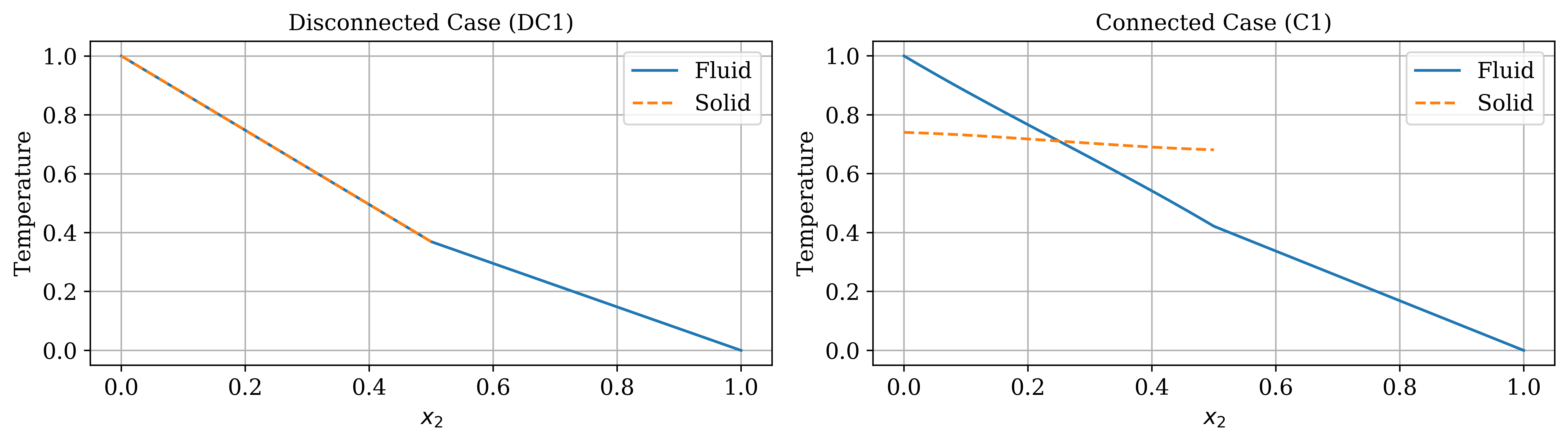
Figure 2: Fluid and solid temperature profile along the $x_{2}$ axis for both models. The pore structures mentioned in tables 1 and 2 are used.

Influence of the pore structure.

To somewhat model our motivating example of a grinding process, where the heat would be produced through the friction between grinding wheel and material, we consider a production term

$$f_{\Sigma}(t,x)=\begin{cases}1,&\text{if }t\leq 10.0\text{ and }x\in\Sigma\\ 0,&\text{otherwise}\end{cases},$$

at the interface. We use this step function in time, to also demonstrate the energy balancing process. In the disconnected case the production $f_{\Sigma}$ can be just added to the interface equation (13e). In the case of a connected structure, we split the production between fluid and solid via the conditions

$$-\kappa^{f}\nabla\theta^{ff}\cdot n_{\Sigma} =-\kappa_{h}^{f}\nabla\theta^{f}\cdot n_{\Sigma}+(1-|\Sigma^{s}|)f_{\Sigma}+\alpha|\Sigma^{s}|(\theta^{s}-\theta^{f}) \text{on}\ \ S\times\Sigma,$$

$$-\kappa_{h}^{s}\nabla\theta^{s}\cdot n_{\Sigma} =\alpha|\Sigma^{s}|(\theta^{s}-\theta^{f})-|\Sigma^{s}|f_{\Sigma} \text{on}\ \ S\times\Sigma.$$

At all outer boundaries a homogeneous Neumann condition is applied.

Again, these condition lead to a one dimensional temperature profile. For this reason we use the same points $\{\mathbf{x}_{i}\}_{i=1}^{11}$, as in the previous section. For comparison, we consider, at different time points $t$, the temperature along the $x_{2}$ axis and the energy inside the subdomains, which correspond to

$$E^{ff}(t)=\int_{\Omega^{ff}}\theta^{ff}(t,x)\,\mathrm{d}x,\quad E^{f}(t)=|Y^{f}|\int_{\Omega^{p}}\theta^{f}(t,x)\,\mathrm{d}x\quad\text{and}\quad E^{s}(t)=|Y^{s}|\int_{\Omega^{p}}\theta^{s}(t,x)\,\mathrm{d}x.$$ (21)

The energy and temperature are presented in figures 3 and 4. One can see, that for the pore geometries (DC1) and (DC2), where the porosity $|Y^{f}|$ is the same, temperature and energy profile almost match. For (DC2) the solid is cooler, since the interface $\Gamma$ is smaller. The structure (DC3) yields more deviations, because of the difference in $|Y^{f}|$ the equilibrium energy distributions are unequal.

The models for connected and disconnected matrices also produce noticeable differences, even when the geometry parameters are the same. Which can be seen by comparing the results for (DC1) and (C1). This is mainly due to the interface production on the solid and possibility of heat diffusion in the connected case. Varying the size of $|\Gamma|$ and $|\Sigma|$ produce expected results, since smaller values correspond to a slower heat transfer into the solid.

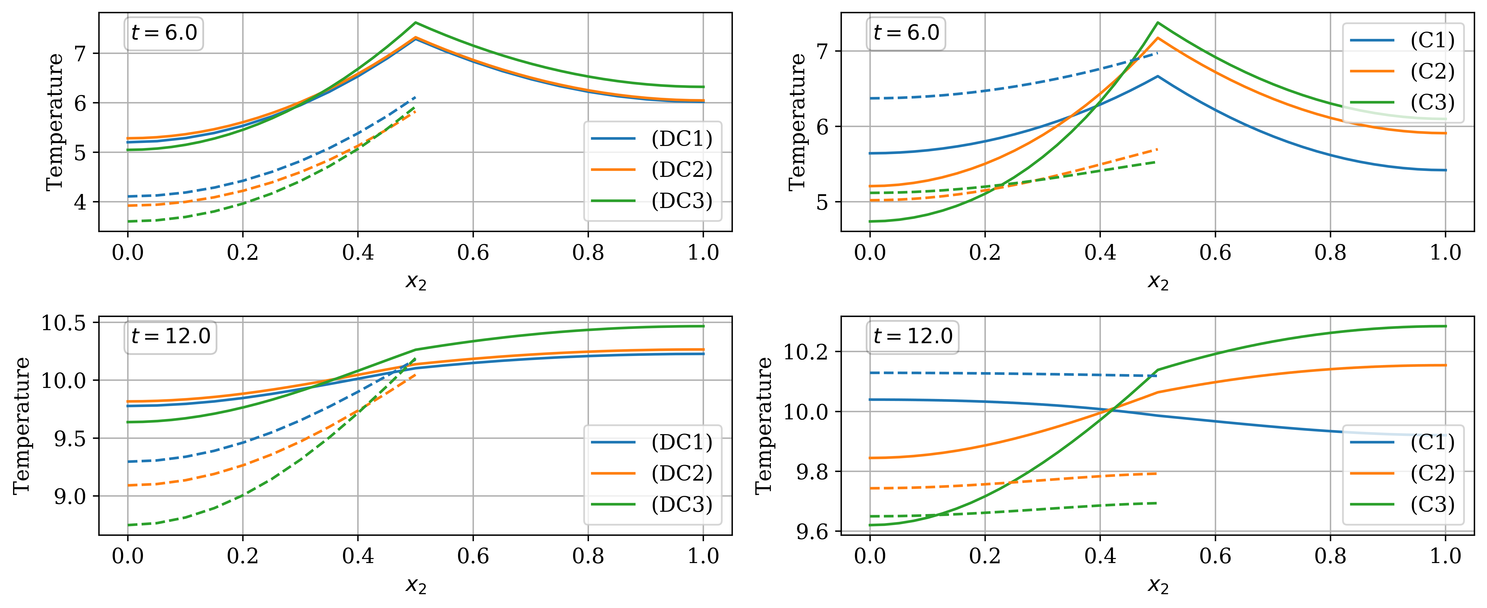
Figure 3: Temperature profiles for different pore structures and at two distinct snap shots in time, along the $x_{2}$ axis. The dashed lines represent the temperatures of the solid.

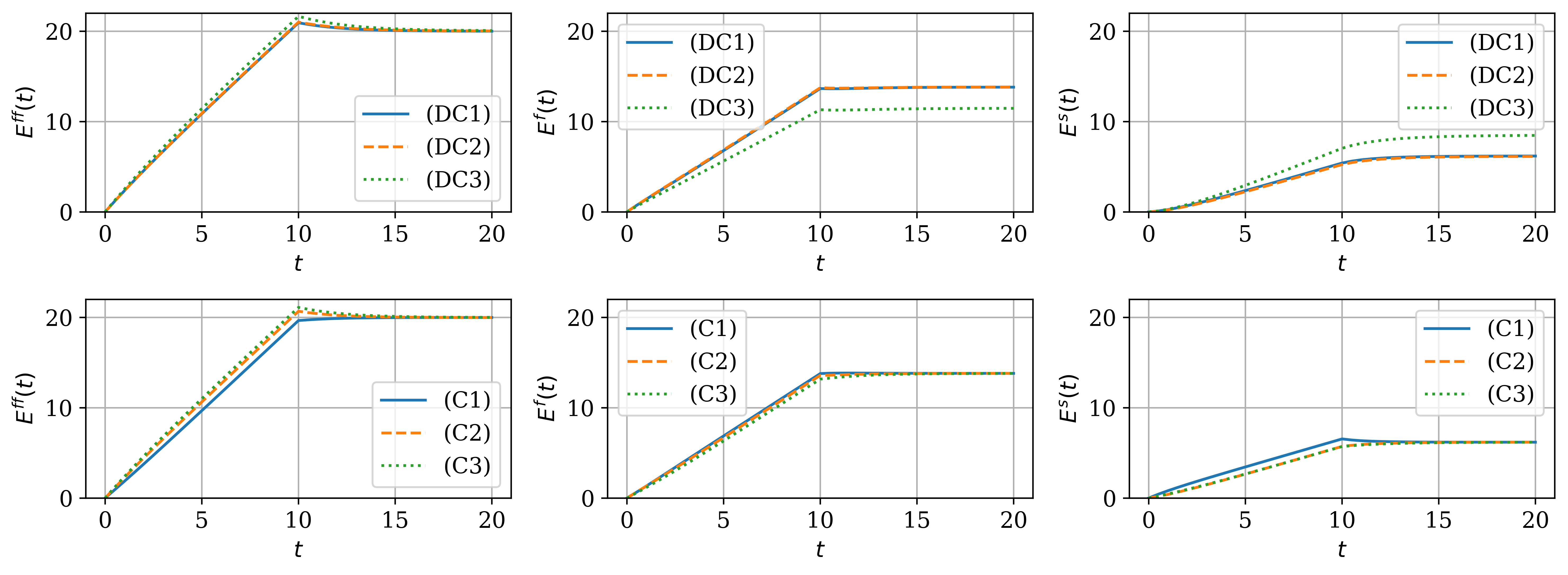
Figure 4: Heat energy (21) inside the different subdomains, for the introduced pore structures in table 1 and 2.

Transition from connected to non connected case.

One question is, whether the results for the connected matrix approach the result of the disconnected case if the connected pore structure transitions to a disconnected one. To examine this aspect, we use the pores (DC1) and (C3) and reduce the side length $c$ while increasing $b$ and keeping $|Y^{f}|$ fixed. The parameters, for different values of $c$, are listed in table 3.

As an comparison we compute the temperature difference between both models in the $L^{2}$-norm, at each time step. For the solid temperature we again use the average (20). The results are shown in figure 5. The expected trend, that for $c\to 0$ both model yield comparable solutions, is visible. It appears to be also possible to just plug the case $c=0$ into the model 4.2 and gain reasonable results. The small difference of around $10^{-3}$, is mainly given by numerical errors regarding energy conservation.

$c$	$b$	$|\Gamma|$	$|\Sigma|$	$\kappa^{f}_{h}/\kappa^{f}$	$\kappa^{s}_{h}/\kappa^{s}$
0.2	0.6437	3.1012	0.04	$0.817I$	$0.251I$
0.1	0.6691	3.0232	0.01	$0.841I$	$0.079I$
0.05	0.6746	2.9108	0.0025	$0.845I$	$0.022I$
0.0	0.6764	2.7451	0.0	$0.848I$	$0.0I$

Table 3: Parameters of (C3) for different side lengths $c$.

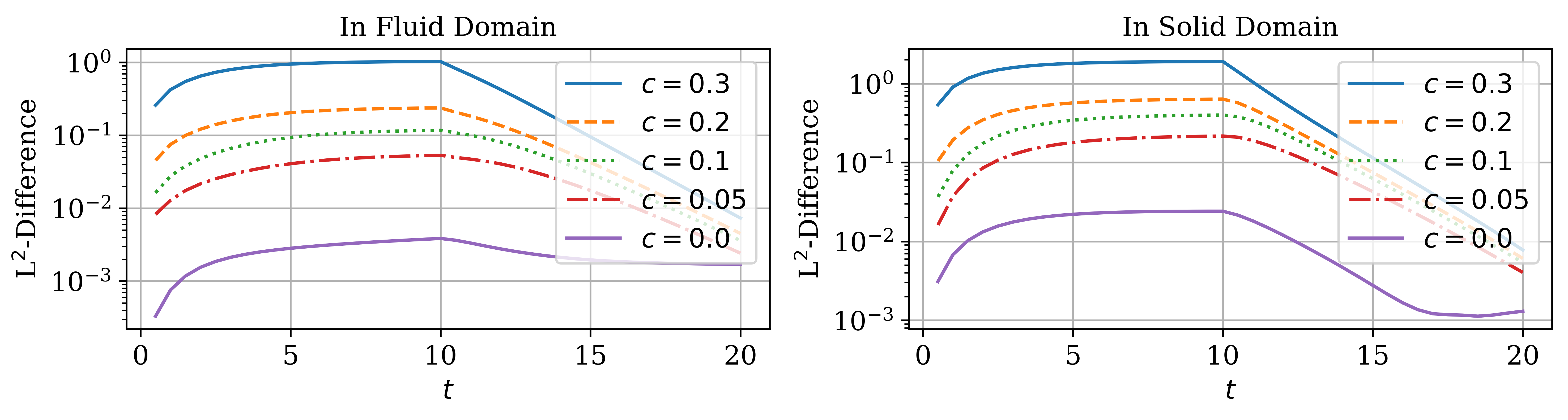
Figure 5: $L^{2}$-difference between the solution of the connected and disconnected cases. Left the fluid temperature, right the solid temperature. Compared are the pore geometries (DC1) and (C3), for different values of $c$.

5.2 Simulations with convection

In the last simulations we will also include some fluid flow. Motivated by engineering applications, where the fluid acts as a coolant, we assume a described inflow temperature and velocity. Additionally we assume, that the influence of the temperature on the flow (e.g. through buoyancy) is negligible and consider a stationary flow profile that has been established before the system heats up.

To compute the fluid flow we use the Navier-Stokes system and the Darcy equation, which is coupled at the interface $\Sigma$ through the Beavers-Joseph conditions [8, 22, 25].

One important parameter for the Darcy equation is the permeability tensor $K$. For a given pore structure, the permeability can be computed via the solutions of problems inside the cell $Y^{f}$ [22]. Some exemplary values are listed in the previous tables 1 and 2.

To further simplify the model and the presentation, we will consider a two dimensional flow and temperature profile, that is constant in the $x_{3}$ direction. As an inflow, we set the two Dirichlet conditions $u^{ff}=(16(x_{2}-0.5)(1-x_{2}),0,0)$ and $\theta^{ff}=0$, if $x_{1}=0$ and $x_{2}\geq 0.5$. On the opposite boundary, at $x_{1}=2$ and $x_{2}\geq 0.5$, we apply a free outflow condition, $(\tfrac{\mu}{2}(\nabla u^{ff}+(\nabla u^{ff})^{T})-p^{ff}I)\cdot\nu=0$, and only allow convective heat transport, $\kappa^{f}\nabla\theta^{ff}\cdot\nu=0$. At all other boundaries, a no-slip condition for the flow and homogeneous Neumann condition for the temperature are used. The viscosity is set to $\mu=1$. Additionally, we apply now an oscillating production: We set ${\tilde{f}_{\Sigma}(t,x)=f_{\Sigma}(2(t\mod{10}),x)}$ and consider the larger time interval $S=[0,50]$.

Again, both the connected and disconnected models will be simulated, where we only consider the geometries (C1) and (DC1). Since the temperature profile will also vary in the $x_{1}$ direction, we solve the cell problems (19) at the points $\{\mathbf{x}_{ij}\}_{i,j=1}^{11}$, with $\mathbf{x}_{ij,1}=\tfrac{j-1}{5},\mathbf{x}_{ij,2}=\tfrac{i-1}{20}$ and $\mathbf{x}_{ij,3}=1$.

The resulting velocity and temperature profiles, at $t=45$, for both model types are presented in figure 6. The difference in the fluid velocity are rather small, especially the flow inside $\Omega^{ff}$. On the other hand, the temperature profiles show noticeable deviations. In the model for the connected matrix, the solid is hotter than in the disconnected case. Additionally, the connected model allows heat diffusion inside the solid, which leads to a stronger counteraction against the heat convection inside the fluid of $\Omega^{p}$.

We also study the influence of the heat exchange value $\alpha$. Where we expect larger $\alpha$ to lead to similar temperature profiles in fluid and solid, smaller values may allow heat to accumulate in the solid domain. The corresponding energy curves for different $\alpha$ values are displayed in figure 7. In the curves for the connected system, we see that the overall energies exactly follow the oscillations of the heat source $\tilde{f}_{\Sigma}$. For small values of $\alpha$ the solid can heat up considerably due to the production on $\Sigma$ and the effect of the coolant is weaker. For the disconnected system the solid is in general a lot cooler than the connected model. Interesting are the cases $\alpha=0.01$ or $0.1$, where the oscillations of heat inside the solid are lagging behind the oscillation of $\tilde{f}_{\Sigma}$ and the energy inside the fluid. Here, we can see the memory effect present in the one-temperature model given in lemma 1. For large $\alpha$ both models exhibit similar results, since a larger heat exchange decreases the ability to store heat inside the solid and, in the connected model, also lessens the impact of heat diffusion in the solid.

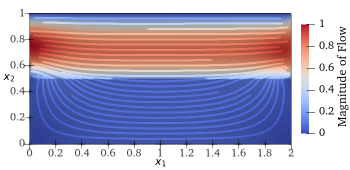
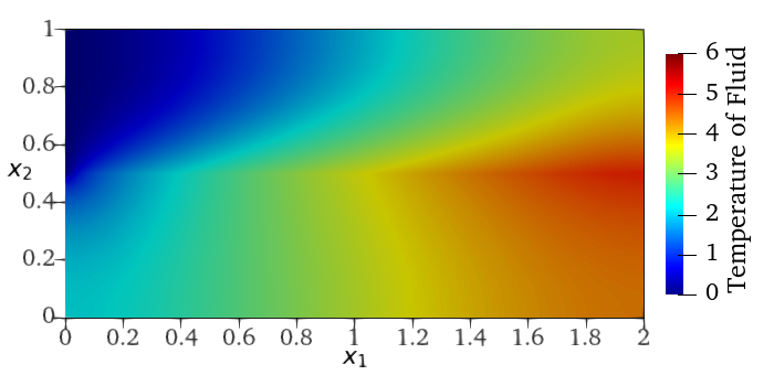
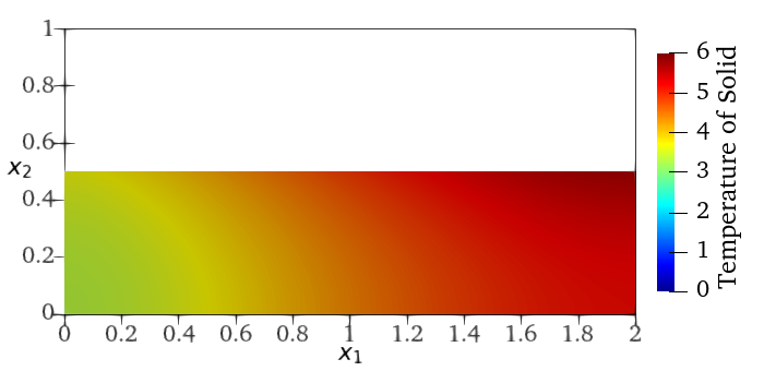
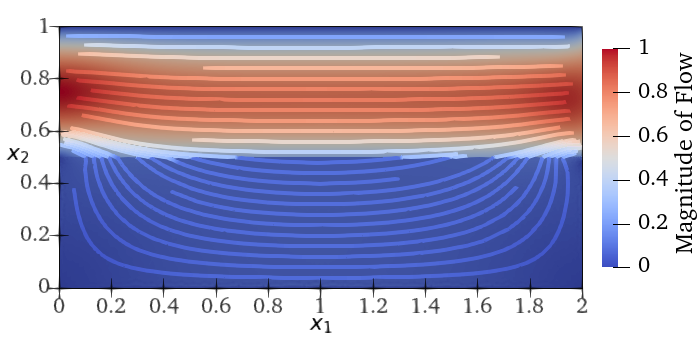
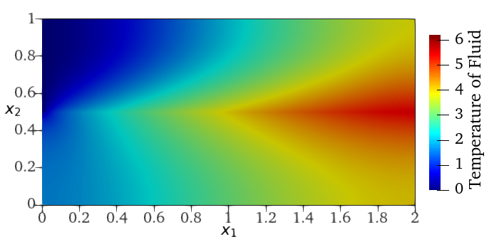
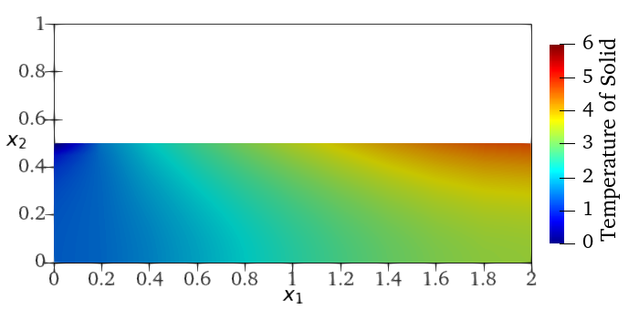
Figure 6: Cross-section of the simulation results. Left: magnitude and streamlines of the flow. Middle and right: the (average) temperature profile at $t=45$ and with $\alpha=0.1$ for the fluid and solid domain respectively. The first row corresponds to the connected system the second to the disconnected system.

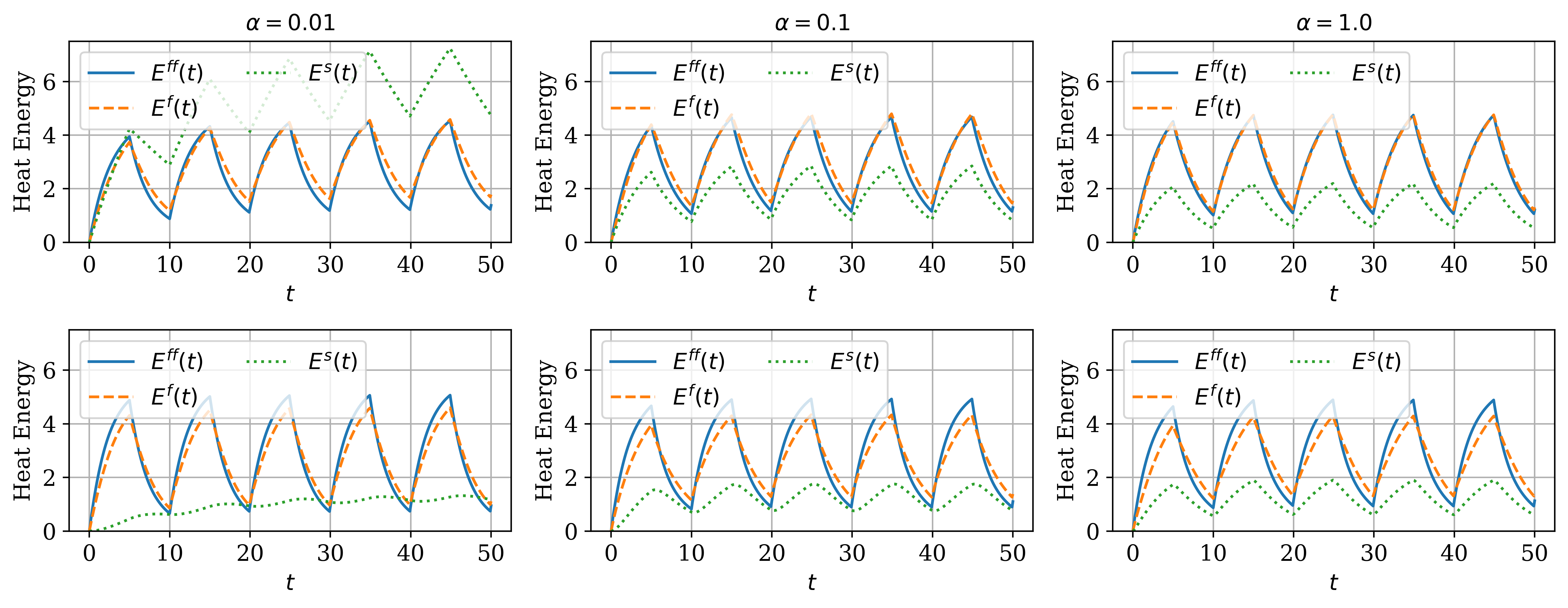
Figure 7: Heat energy (21) plotted over time, for different $\alpha$, the system with convection and an oscillating heat source. Each column shows the results for different heat exchange values $\alpha$, the first row corresponds to the connected system the second to the disconnected system.

References

- [1] C. G. Aguilar-Madera, F. J. Valdés-Parada, B. Goyeau, and J. Alberto Ochoa-Tapia, One-domain approach for heat transfer between a porous medium and a fluid, Int. J. Heat Mass Transfer, 54 (2011), pp. 2089–2099.
- [2] A. Ainouz, Homogenization of a double porosity model in deformable media, Electron. J. Differential Equations, 2013 (2012).
- [3] B. Alazmi and K. Vafai, Analysis of fluid flow and heat transfer interfacial conditions between a porous medium and a fluid layer, Int. J. Heat Mass Transfer, 44 (2001), pp. 1735–1749.
- [4] A. Alhusseny, Q. Al-Aabidy, N. Al-Zurfi, A. Nasser, and M. Aljanabi, Cooling of high-performance electronic equipment using graphite foam heat sinks, Appl. Therm. Eng., 191 (2021), p. 116844.
- [5] G. Allaire, Homogenization and two scale convergence, SIAM J. Math. Anal., 23 (1992), pp. 1482–1518.
- [6] M. S. Alnaes, J. Blechta, J. Hake, A. Johansson, B. Kehlet, A. Logg, C. Richardson, J. Ring, M. E. Rognes, and G. N. Wells, The FEniCS project version 1.5, Arch. Num. Soft., 3 (2015).
- [7] T. Arbogast, J. Douglas, Jim, and U. Hornung, Derivation of the double porosity model of single phase flow via homogenization theory, SIAM J. Math. Anal., 21 (1990-07), pp. 823–836.
- [8] G. S. Beavers and D. D. Joseph, Boundary conditions at a naturally permeable wall, J. Math. Fluid Mech., 30 (1967), pp. 197–207.
- [9] A. Bourgeat, S. Luckhaus, and A. Mikelić, Convergence of the homogenization process for a double-porosity model of immiscible two-phase flow, SIAM J. Math. Anal., 27 (1996), pp. 1520–1543.
- [10] D. Cioranescu and J. Saint Jean Paulin, Homogenization of reticulated structures, vol. 136 of Applied Mathematical Sciences, Springer-Verlag, New York, 1999.
- [11] M. Eden and M. Böhm, Homogenization of a poro-elasticity model coupled with diffusive transport and a first order reaction for concrete, Netw. Heterog. Media, 9 (2014), pp. 599–615.
- [12] M. Eden and H. S. Mahato, Homogenization of a poroelasticity model for fiber-reinforced hydrogels, Math. Methods Appl. Sci., 45 (2022), pp. 11562–11580.
- [13] M. Eden and A. Muntean, Homogenization of a fully coupled thermoelasticity problem for a highly heterogeneous medium with a priori known phase transformations, Math. Methods Appl. Sci., 40 (2017), pp. 3955–3972.
- [14] E. Eggenweiler and I. Rybak, Effective coupling conditions for arbitrary flows in Stokes-Darcy systems, Multiscale Model. Simul., 19 (2021), pp. 731–757.
- [15] H. I. Ene, C. Timofte, and I. Ţenţea, Homogenization of a thermoelasticity model for a composite with imperfect interface, Bull. Math. Soc. Sci. Math. Roumanie (N.S.), 58 (106) (2015), pp. 147–160.
- [16] M. Gahn, M. Neuss-Radu, and I. S. Pop, Homogenization of a reaction-diffusion-advection problem in an evolving micro-domain and including nonlinear boundary conditions, J. of Differential Equations, 289 (2021), pp. 95–127.
- [17] C. Geuzaine and J.-F. Remacle, Gmsh: A 3-d finite element mesh generator with built-in pre- and post-processing facilities, Int. J. Numer. Methods. Eng., 79 (2009), pp. 1309 – 1331.
- [18] I. Graf and M. A. Peter, Homogenization of fast diffusion on surfaces with a two-step method and an application to -cell signaling, Nonlinear Anal. Real World Appl., 17 (2014), pp. 344–364.
- [19] I. Graf, M. A. Peter, and J. Sneyd, Homogenization of a nonlinear multiscale model of calcium dynamics in biological cells, J. Math. Anal. Appl., 419 (2014), pp. 28–47.
- [20] I. Gruais and D. Poliševski, Model of two-temperature convective transfer in porous media, Z. Angew. Math. Phys., 68 (2017), p. 143.
- [21] M. Höpker and M. Böhm, A note on the existence of extension operators for Sobolev spaces on periodic domains, C. R. Math. Acad. Sci. Paris, 352 (2014), pp. 807–810.
- [22] U. Hornung, Homogenization and Porous Media, Springer New York, 1997.
- [23] U. Hornung and W. Jäger, Diffusion, convection, adsorption, and reaction of chemicals in porous media, J. of Differential Equations, 92 (1991), pp. 199–225.
- [24] D. Jamet and M. Chandesris, On the intrinsic nature of jump coefficients at the interface between a porous medium and a free fluid region, Int. J. Heat Mass Transfer, 52 (2009), pp. 289–300.
- [25] W. Jäger and A. Mikelić, On the interface boundary condition of Beavers, Joseph, and Saffman, SIAM J. Appl. Math., 60 (2000), pp. 1111–1127.
- [26] D. Lukkassen, G. Nguetseng, and P. Wall, Two-scale convergence, Int. J. Pure Appl. Math., 2 (2002), pp. 35–86.
- [27] A. Marciniak-Czochra and A. Mikelić, Effective pressure interface law for transport phenomena between an unconfined fluid and a porous medium using homogenization, Multiscale Model. Simul., 10 (2012), pp. 285–305.
- [28] M. Neuss-Radu, Some extensions of two-scale convergence, C. R. Acad. Sci. Paris Sér. I Math., 322 (1996), pp. 899–904.
- [29] D. A. Nield, A note on local thermal non-equilibrium in porous media near boundaries and interfaces, Transp. Porous Media, 95 (2012), pp. 581–584.
- [30] J. A. Ochoa-Tapia and S. Whitaker, Heat transfer at the boundary between a porous medium and a homogeneous fluid: the one-equation model, J. Porous Media, 1 (1998).
- [31] G. A. Pavliotis and A. M. Stuart, Multiscale methods, vol. 53 of Texts in Applied Mathematics, Springer, New York, 2008.
- [32] M. Peszyńska, R. E. Showalter, and S.-Y. Yi, Flow and transport when scales are not separated: numerical analysis and simulations of micro- and macro-models, Int. J. Numer. Anal. Model., 12 (2015), pp. 476–515.
- [33] M. Prat, Modelling of heat transfer by conduction in a transition region between a porous medium and an external fluid, Transp. Porous Med., 5 (1990), pp. 71–95.
- [34] M. Sahraoui and M. Kaviany, Slip and no-slip temperature boundary conditions at the interface of porous, plain media: Convection, Int. J. Heat Mass Transfer, 37 (1994), pp. 1029–1044.
- [35] R. E. Showalter and D. B. Visarraga, Double-diffusion models from a highly-heterogeneous medium, J. Math. Anal. Appl., 295 (2004), pp. 191–210.
- [36] C. Taylor and P. Hood, A numerical solution of the Navier-Stokes equations using the finite element technique, Comput. & Fluids, 1 (1973), pp. 73–100.
- [37] K. Vafai and R. Thiyagaraja, Analysis of flow and heat transfer at the interface region of a porous medium, Int. J. Heat Mass Transfer, 30 (1987), pp. 1391–1405.
- [38] S. Whitaker, The Method of Volume Averaging, vol. 13 of Theory and Applications of Transport in Porous Media, Springer Netherlands, 1999.
- [39] F. Wiesener, B. Bergmann, M. Wichmann, M. Eden, T. Freudenberg, and A. Schmidt, Modeling of heat transfer in tool grinding for multiscale simulations. submitted (in revision), 2022.
- [40] K. Yang and K. Vafai, Restrictions on the validity of the thermal conditions at the porous-fluid interface: an exact solution, J. Heat Transfer, 133 (2011).