An empirical spectroscopic model for eleven electronic states of VO

Abstract

Previously-determined empirical energy levels are used to construct a rovibronic model for the $\mathrm{X}\,^{4}\Sigma^{-}$, $\mathrm{A}^{\prime}\,{}^{4}\Phi$, $\mathrm{A}\,^{4}\Pi$, $\mathrm{B}\,^{4}\Pi$, $\mathrm{C}\,^{4}\Sigma^{-}$, $\mathrm{D}\,^{4}\Delta$, $\mathrm{1}\,^{2}\Delta$, $\mathrm{1}\,^{2}\Sigma^{+}$, $\mathrm{1}\,^{2}\Phi$, $\mathrm{1}\,^{2}\Pi$ and $\mathrm{2}\,^{2}\Pi$ electronic states of vanadium mononoxide. The spectrum of VO is characterized by many couplings and crossings between the states associated with these curves. The model is based on the use of potential energy curves, represented as extended Morse oscillators, and couplings (spin-orbit, spin-spin, angular momentum), represented by polynomials, which are tuned to the data plus an empirical allowance for spin-rotation couplings. The curves are used as input for the variational nuclear motion code Duo. For the $\mathrm{X}\,^{4}\Sigma^{-}$, $\mathrm{1}\,^{2}\Phi$ and $\mathrm{1}\,^{2}\Pi$ states the model reproduces the observed energy to significantly better than 0.1 cm^-1. For the other states the standard deviations are between 0.25 and 1.5 cm^-1. Further experimental data and consideration of hyperfine effects would probably be needed to significantly improve this situation.

[UCL]organization=Department of Physics and Astronomy, University College London,city=London, postcode=WC1E 6BT, country=United Kingdom

1 Introduction

Vanadium monoxide (VO) is a diatomic molecule with a complicated open shell structure [1, 2]; it absorbs strongly at red and near infrared wavelengths. VO is thought to provide an important source of opacity in the atmospheres of both cool stars [3] and of exoplanets [4, 5]. While VO bands are well-know in the spectrum of cool stars [6] and sunspots [7], only tentative detections have been made in the atmospheres of exoplanets [8, 9, 10, 11, 12, 13, 14]. The charged species VO^- and VO^+ are also important targets of theoretical and experimental studies, see e.g., Miliordos and Mavridis [15] and the references therein.

Theoretically modelling of VO spectra is a challenge both from the perspective of electronic structure calculations [16, 15, 17, 18] and, as will be seen below, from the perspective of representing the nuclear motion due to many resonances between different states. McKemmish et al. [19] constructed the so-called VOMYT line list for VO as part of the ExoMol project [20, 21]. The VOMYT line list probably provides a reasonable basis for modelling VO opacities but has been demonstrated to be inadequate for high resolution studies of exoplanetary spectra [22].

The spectrum of VO has been well-studied experimentally [23, 24, 25, 26, 27, 28, 29, 30, 31, 32, 33, 34, 35], see the summary by Bowesman et al. [36]; however, the complexity of its spectrum means that there are still important gaps in these studies. Although, as discussed below, our general approach to constructing a spectroscopic model for open shell molecules such as VO is based on variational solutions of the nuclear motion Schrodinger equation, our work on VO [2, 36] and other open shell molecules [37, 38, 39, 40] has made extensive use of Western’s effective Hamiltonian program PGOPHER [41]. We favour the method based on variational solutions as it usually shows much more stable extrapolation properties which is an important feature when one wishes to compute line lists for hot molecules.

In this paper, we attempt to build a spectroscopic model which covers the most important low-lying states of VO, including 6 quartet and 5 doublet electronic states; given the difficulty in fully characterizing the couplings between these state we limit ourselves to considering only the coupling terms necessary to provide a reasonable spectroscopic model. The 11 electronic states considered are shown in Fig. 1; these state are all part of the VOMYT model. They are responsible for the main absorption bands in the near infrared and visible, or are states which are known to interact with them.

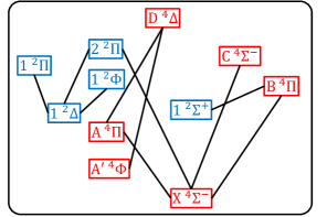
Figure 1: Band systems connecting the 11 electronics included in the model of this work. See Bowesman et al. [36] for a more comprehensive diagram.

The purpose of this work is to provide the basis for a more reliable model than VOMYT as well providing for the quantum number assignments for unassigned recent observations [35, 36]. Thus, our focus is on the accuracy of energy levels and we develop an empirical model that excludes most of the off-diagonal couplings considered in VOMYT [19]. In the recent study by Bowesman et al. [36], a spectroscopic network of VO transitions was constructed as a prelude to a MARVEL (measured active rotation vibration energy levels) [42] study of the 11 states involved in this network. The next two sections will demonstrate our effort to reproduce the rovibronic energy levels obtained from the MARVEL study. The other two states ($\mathrm{a}\,^{2}\Sigma^{-}$ and $\mathrm{b}\,^{2}\Gamma$ ) included in VOMYT [19] were not analyzed in the work of Bowesman et al. [36] and are, therefore, excluded from our model as well.

2 Spectroscopic model

The model was developed using the open-source program for variational calculation of diatomic spectra, Duo [43]. All nuclear motion calculations used 10 vibrationally contracted basis functions for each electronic states based on 401 sinc-DVR grid points, covering the internuclear distance range from 1.2 to 4 $\mathrm{\SIUnitSymbolAngstrom}$. The upper bound of the energy was set to $50\,000\text{\,}{\mathrm{cm}}^{-1}$, however energy levels of interest for this work are expected to be below $21\,000\text{\,}{\mathrm{cm}}^{-1}$. The number of vibrational levels considered for each electronic state is listed in Table 1.

Table 1: Vibrational states considered for each electronic state. Table 5 of Bowesman et al. [36] lists the corresponding experimental studies.

Number	States	$v$
1	$\mathrm{X}\,^{4}\Sigma^{-}$	0-2
2	$\mathrm{A}^{\prime}\,{}^{4}\Phi$	0-2
3	$\mathrm{A}\,^{4}\Pi$	0
4	$\mathrm{B}\,^{4}\Pi$	0-1
5	$\mathrm{C}\,^{4}\Sigma^{-}$	0-2
6	$\mathrm{D}\,^{4}\Delta$	0-1
9	$\mathrm{1}\,^{2}\Delta$	0-1
10	$\mathrm{1}\,^{2}\Sigma^{+}$	2-3
11	$\mathrm{1}\,^{2}\Phi$	0
12	$\mathrm{1}\,^{2}\Pi$	0-3
13	$\mathrm{2}\,^{2}\Pi$	0-1

2.1 Potential energy curves

The potential energy curves (PECs) of all states are represented by second-order extended Morse oscillator (EMO) function [44]

$$V(R)=T_{\mathrm{e}}+\left(D_{\mathrm{e}}-T_{\mathrm{e}}\right)\left[1-\exp\left(-\beta_{\mathrm{EMO}}(R)\left(R-R_{\mathrm{e}}\right)\right)\right]^{2},$$ (1)

where $R$ is the internuclear distance, $R_{\mathrm{e}}$ is the equilibrium bond length and $T_{\mathrm{e}}$ is the potential minimum; $\beta_{\mathrm{EMO}}$ is given by the formula:

$$\beta_{\mathrm{EMO}}(R)=b_{0}+b_{1}\,y_{p}(R)+b_{2}\,y_{p}^{2}(R),$$ (2)

where $y_{p}(R)$ is:

$$y_{p}(R)=\frac{R^{p}-(R_{\mathrm{e}})^{p}}{R^{p}+(R_{\mathrm{e}})^{p}}\,.$$ (3)

Duo’s users can set independent integer values of $p$ on the left- and right-hand sides of $R_{\mathrm{e}}$ and we chose $p=4$ for both sides. The parameters of fitted EMO functions are listed in Table 2.

Table 2: Optimized extended Morse oscillator (EMO) parameters for the potential energy curves, see Eq.(1).

Number	State	$T_{\mathrm{e}}$ [${\mathrm{cm}}^{-1}$]	$R_{\mathrm{e}}$ [$\mathrm{\SIUnitSymbolAngstrom}$]	$b_{0}$ [${\mathrm{\SIUnitSymbolAngstrom}}^{-1}$]	$b_{1}$ [${\mathrm{\SIUnitSymbolAngstrom}}^{-1}$]	$b_{2}$ [${\mathrm{\SIUnitSymbolAngstrom}}^{-1}$]
1	$\mathrm{X}\,^{4}\Sigma^{-}$	0	1.58947260	1.87183393	$6.042\,606\,63\text{\times}{10}^{-03}$	$-1.158\,731\,02\text{\times}{10}^{-01}$
2	$\mathrm{A}^{\prime}\,{}^{4}\Phi$	7292.4851	1.62591915	1.88461684	$-1.332\,091\,48\text{\times}{10}^{-02}$	$1.585\,203\,16\text{\times}{10}^{-01}$
3	$\mathrm{A}\,^{4}\Pi$	9534.8342	1.63405670	1.92275217
4	$\mathrm{B}\,^{4}\Pi$	12659.4107	1.64032109	1.93810207	0	$-2.273\,213\,32\text{\times}{10}^{-01}$
5	$\mathrm{C}\,^{4}\Sigma^{-}$	17494.4977	1.67098029	1.94981612	$-5.170\,578\,88\text{\times}{10}^{-02}$	$3.271\,206\,99\text{\times}{10}^{-01}$
6	$\mathrm{D}\,^{4}\Delta$	19238.8720	1.68337218	1.91485252	0	3.03001473
7	$\mathrm{1}\,^{2}\Delta$	9867.6920	1.58225344	2.06276090	0	$-4.155\,158\,02\text{\times}{10}^{-01}$
8	$\mathrm{1}\,^{2}\Sigma^{+}$	10376.3396	1.57856000	2.15102878	0	$-3.663\,042\,53\text{\times}{10}^{-01}$
9	$\mathrm{1}\,^{2}\Phi$	15442.9452	1.62904530	2.09925561
10	$\mathrm{1}\,^{2}\Pi$	17099.9353	1.62955854	2.10656122	$2.732\,894\,47\text{\times}{10}^{-01}$	$1.641\,222\,98\text{\times}{10}^{-01}$
11	$\mathrm{2}\,^{2}\Pi$	18139.4421	1.62244306	2.15748234

2.2 Diagonal couplings within a electronic state

All coupling curves are represented by low-order polynomials

$$p(R)=a_{0}+\sum_{n=1}^{\dots}a_{n}\,(R-R_{\mathrm{e}})^{n}.$$ (4)

Our aim is to use the fewest terms to satisfactorily reproduce the experimental energy levels. Thus, we started with uncoupled PECs for each state and then, added those couplings curves necessary to reduce the fitting errors.

We assume the spin splittings of $\mathrm{X}\,^{4}\Sigma^{-}$ and $\mathrm{C}\,^{4}\Sigma^{-}$ mainly depend on spin-spin coupling terms. Although the assumption is not supported by ab initio calculations, e.g. see our previous discussion of the $\mathrm{X}\,^{4}\Sigma^{-}$ state[2], this empirical representation can usually give accurate energy levels. Apart from the spin-spin interaction, spin-rotation terms were used to resolve $J$-dependent spin splittings of ${}^{2}\Sigma$ and ${}^{4}\Sigma$ states, where $J$ is the total angular momentum.

In contrast, spin-orbit terms dominate the spin splittings of $\Pi$, $\Delta$, $\Phi$ and $\Gamma$ states and are $J$-dependent too. Therefore, we replaced spin-rotation curves with spin-orbit coupling ones for those states. Spin-spin coupling curves were still used for the quartet states, i.e. $\mathrm{A}^{\prime}\,{}^{4}\Phi$, $\mathrm{A}\,^{4}\Pi$, $\mathrm{B}\,^{4}\Pi$ and $\mathrm{D}\,^{4}\Delta$.

The optimized parameters of diagonal spin-spin, spin-rotation and spin-orbit couplings are listed in Tables 3, 4 and 5, respectively.

Table 3: Optimized polynomial parameters for diagonal spin-spin coupling curves.

State	$a_{0}$ [${\mathrm{cm}}^{-1}$]	$a_{1}$ [${\mathrm{cm}}^{-1}\text{\,}{\mathrm{\SIUnitSymbolAngstrom}}^{-1}$]	$a_{2}$ [$\mathrm{c}\mathrm{m}^{-1}\mathrm{\SIUnitSymbolAngstrom}^{-2}$]
$\mathrm{X}\,^{4}\Sigma^{-}$	2.05042406	2.76918955
$\mathrm{A}^{\prime}\,{}^{4}\Phi$	-1.08746355
$\mathrm{A}\,^{4}\Pi$	1.89104909
$\mathrm{B}\,^{4}\Pi$	2.62698261
$\mathrm{C}\,^{4}\Sigma^{-}$	0.73293575
$\mathrm{D}\,^{4}\Delta$	1.29783687	0	$-6.220\,435\,54\text{\times}{10}^{02}$

Table 4: Optimized polynomial parameters for diagonal spin-rotation coupling curves.

State	$a_{0}$ [${\mathrm{cm}}^{-1}$]	$a_{1}$ [$\mathrm{c}\mathrm{m}^{-1}\mathrm{\SIUnitSymbolAngstrom}^{-1}$]
$\mathrm{X}\,^{4}\Sigma^{-}$	$2.143\,878\,41\text{\times}{10}^{-02}$	$1.587\,127\,88\text{\times}{10}^{-01}$
$\mathrm{C}\,^{4}\Sigma^{-}$	$-1.834\,643\,08\text{\times}{10}^{-02}$
$\mathrm{1}\,^{2}\Sigma^{+}$	$-7.900\,000\,00\text{\times}{10}^{-03}$

Table 5: Optimized polynomial parameters for diagonal spin-orbit coupling curves.

State	$a_{0}$ [${\mathrm{cm}}^{-1}$]	$a_{1}$ [${\mathrm{cm}}^{-1}\text{\,}{\mathrm{\SIUnitSymbolAngstrom}}^{-1}$]	$a_{2}$ [$\mathrm{c}\mathrm{m}^{-1}\mathrm{\SIUnitSymbolAngstrom}^{-2}$]	$a_{3}$[$\mathrm{c}\mathrm{m}^{-1}\mathrm{\SIUnitSymbolAngstrom}^{-3}$]
$\mathrm{A}^{\prime}\,{}^{4}\Phi$	$2.607\,527\,43\text{\times}{10}^{02}$	$-3.083\,775\,40\text{\times}{10}^{02}$	$-3.019\,871\,04\text{\times}{10}^{03}$	$5.206\,561\,86\text{\times}{10}^{04}$
$\mathrm{A}\,^{4}\Pi$	$5.264\,954\,55\text{\times}{10}^{01}$
$\mathrm{B}\,^{4}\Pi$	$9.703\,432\,61\text{\times}{10}^{01}$	$-3.312\,045\,51\text{\times}{10}^{01}$
$\mathrm{D}\,^{4}\Delta$	$1.390\,545\,88\text{\times}{10}^{02}$	0	$2.599\,205\,12\text{\times}{10}^{03}$
$\mathrm{1}\,^{2}\Delta$	$1.800\,558\,32\text{\times}{10}^{02}$	$-1.587\,723\,00\text{\times}{10}^{02}$
$\mathrm{1}\,^{2}\Phi$	$1.860\,528\,51\text{\times}{10}^{02}$
$\mathrm{1}\,^{2}\Pi$	$1.245\,874\,33\text{\times}{10}^{02}$	$8.268\,778\,79\text{\times}{10}^{01}$	$-2.704\,796\,01\text{\times}{10}^{02}$
$\mathrm{2}\,^{2}\Pi$	$6.037\,144\,58\text{\times}{10}^{01}$

We also modeled the $\varLambda$ - doubling of $\Pi$ states by using the empirical terms defined by Brown and Merer [45]:

$$\matrixelement{\mp 1,\varSigma\pm 2,J,\varOmega}{\hat{H}_{\mathrm{LD}}}{\pm 1,\varSigma,J,\varOmega}=\frac{1}{2}\left(o_{v}+p_{v}+q_{v}\right)\times$$

$$\sqrt{[S(S+1)-\varSigma(\varSigma\pm 1)][S(S+1)-(\varSigma\pm 1)(\varSigma\pm 2)]}\,,$$ (5)

$$\matrixelement{\mp 1,\varSigma\pm 1,J,\varOmega\mp 1}{\hat{H}_{\mathrm{LD}}}{\pm 1,\varSigma,J,\varOmega}=-\frac{1}{2}\left(p_{v}+2q_{v}\right)\times$$

$$\sqrt{[S(S+1)-\varSigma(\varSigma\pm 1)][J(J+1)-\varOmega(\varOmega\mp 1)]}\,,$$ (6)

$$\matrixelement{\mp 1,\varSigma,J,\varOmega\mp 2}{\hat{H}_{\mathrm{LD}}}{\pm 1,\varSigma,J,\varOmega}=\frac{1}{2}q_{v}\times$$

$$\sqrt{[J(J+1)-\varOmega(\varOmega\mp 1)][J(J+1)-(\varOmega\mp 1)(\varOmega\mp 2)]}\,.$$ (7)

In these equations, $o$, $p$ and $q$ depend on vibrational quantum number, $v$, as Brown and Merer derived the equations based on effective Hamiltonians. In our variational model, we use coupling curves instead. For quartet states, we include all the three coupling curves, while for doublet states, Eq. (5) is automatically zero and we only need the curves of $p+2q$ and $q$. The fitted parameters for the $o+p+q$, $p+2q$ and $q$ curves are listed in Table 6.

Table 6: Optimized polynomial parameters for the $o+p+q$, $p+2q$ and $q$ curves due to $\varLambda$ - doubling coupling.

Coupling	State	$a_{0}$ [${\mathrm{cm}}^{-1}$]
$o+p+q$	$\mathrm{A}\,^{4}\Pi$	2.05253781
	$\mathrm{B}\,^{4}\Pi$	1.20113529
$p+2q$	$\mathrm{A}\,^{4}\Pi$	$-1.416\,923\,02\text{\times}{10}^{-02}$
	$\mathrm{B}\,^{4}\Pi$	$3.189\,748\,36\text{\times}{10}^{-02}$
	$\mathrm{1}\,^{2}\Pi$	$-3.121\,071\,39\text{\times}{10}^{-02}$
	$\mathrm{2}\,^{2}\Pi$	$-2.196\,020\,31\text{\times}{10}^{-02}$
$q$	$\mathrm{A}\,^{4}\Pi$	$-2.092\,792\,99\text{\times}{10}^{-04}$
	$\mathrm{B}\,^{4}\Pi$	$-1.633\,370\,99\text{\times}{10}^{-04}$
	$\mathrm{1}\,^{2}\Pi$	$-2.043\,450\,34\text{\times}{10}^{-04}$
	$\mathrm{2}\,^{2}\Pi$	$1.002\,402\,89\text{\times}{10}^{-03}$

2.2.1 Off-diagonal spin-orbit couplings

We can observe obvious avoided-crossing structures from the rovibronic energy distributions of $\mathrm{B}\,^{4}\Pi-\mathrm{1}\,^{2}\Sigma^{+}$ and $\mathrm{C}\,^{4}\Sigma^{-}-\mathrm{2}\,^{2}\Pi$ coupled states. Thus, off-diagonal spin-orbit coupling curves, whose parameters are given in Table 7, were introduced to model those structures in crossing regions. The $\mathrm{B}\,^{4}\Pi-\mathrm{1}\,^{2}\Sigma^{+}$ spin-orbit coupling term was optimized using Duo, while the $\mathrm{C}\,^{4}\Sigma^{-}-\mathrm{2}\,^{2}\Pi$ coupling was manually given an estimated value. See the next section where the results are discussed.

Table 7: Polynomial parameters for the off-diagonal spin-orbit coupling curves.

State	$a_{0}$ [${\mathrm{cm}}^{-1}$]
$\mathrm{B}\,^{4}\Pi-\mathrm{1}\,^{2}\Sigma^{+}$	$21.510\,737\,9$
$\mathrm{C}\,^{4}\Sigma^{-}-\mathrm{2}\,^{2}\Pi$	10

3 Results

3.1 Uncoupled states

The fitting residues of the uncoupled quartet states are given in Fig. 2. The energy levels of $\mathrm{X}\,^{4}\Sigma^{-}$ and $\mathrm{A}\,^{4}\Pi$ are accurately reproduced. Compared with the $\mathrm{X}\,^{4}\Sigma^{-}$ and $\mathrm{A}\,^{4}\Pi$ states, the spin-splittings of $\mathrm{A}^{\prime}\,{}^{4}\Phi$ and $\mathrm{D}\,^{4}\Delta$ are not well estimated which may arise from electronic state interactions not included in our model. However, the assignment will not be affected as the energy gaps due to spin-orbit couplings of $\mathrm{A}^{\prime}\,{}^{4}\Phi$ and $\mathrm{D}\,^{4}\Delta$ are usually more than a hundred wavenumbers.

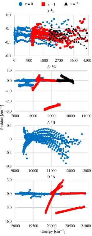
Figure 2: Fitting residues of four uncoupled quartet states: $\mathrm{X}\,^{4}\Sigma^{-}$, $\mathrm{A}^{\prime}\,{}^{4}\Phi$, $\mathrm{A}\,^{4}\Pi$ and $\mathrm{D}\,^{4}\Delta$.

The fitting residues of the uncoupled doublet states are shown in Fig. 3. The doublet states only have two fine structure series which makes it easier to get good refinement results. The errors for the high-$J$ levels of $\mathrm{1}\,^{2}\Delta$ increase dramatically which is also due to state interactions.

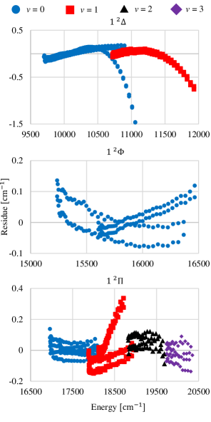
Figure 3: Fitting residues of three uncoupled doublet states: $\mathrm{1}\,^{2}\Delta$, $\mathrm{1}\,^{2}\Phi$ and $\mathrm{1}\,^{2}\Pi$.

3.2 Coupled states

In our model, $\mathrm{B}\,^{4}\Pi-\mathrm{1}\,^{2}\Sigma^{+}$ and $\mathrm{C}\,^{4}\Sigma^{-}-\mathrm{2}\,^{2}\Pi$ are coupled by spin-orbit terms to give reasonable avoided crossing structures, as shown from Fig. 4 to Fig. 7.

Figures 4 and 5 demonstrate the smooth transitions from on electronic state to another in both $e$ and $f$ series. Note that, the electronic state quantum numbers of the energy levels near the interaction region are not well-determined. They are assigned according to the dominant contribution of the corresponding basis function to the rovibronic wavefunction. The MARVEL energy levels indicated by the black arrows in these figures were excluded from the fits. They seems belong to another electronic state but were not recognized in the current model.

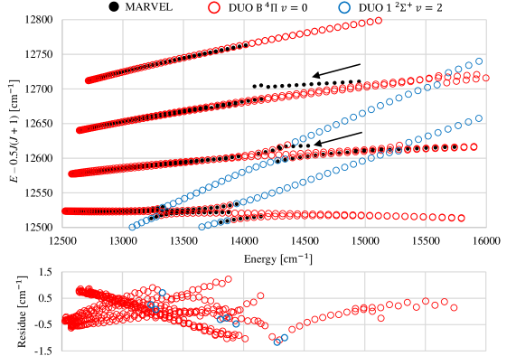
Figure 4: State interaction of $\mathrm{B}\,^{4}\Pi,v=0$ and $\mathrm{1}\,^{2}\Sigma^{+},v=2$. The black dots in the top panel are the rovibronic energy levels obtained from MARVEL analysis [36] while the circles are the fitting results of Duo. The black arrows indicate some unreasonable data which were excluded in our fitting. The bottom panel shows the fitting residues.

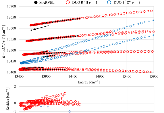
Figure 5: State interaction of $\mathrm{B}\,^{4}\Pi,v=1$ and $\mathrm{1}\,^{2}\Sigma^{+},v=3$. The black dots in the top panel are the rovibronic energy levels obtained from MARVEL analysis [36] while the circles are the fitting results of Duo. The bottom panel shows the fitting residues.

The off-diagonal $\mathrm{C}\,^{4}\Sigma^{-}-\mathrm{2}\,^{2}\Pi$ spin-orbit coupling term was not fitted but visually estimated to give an acceptable avoided-crossing structure as shown in Figs. 6 and 7. The $v=0,F_{2}$ levels of $\mathrm{2}\,^{2}\Pi$ shown in Fig. 6 are recently assigned in the work of Bowesman et al. [36]. However, the crossing point of this series with $F_{2}$ series of $\mathrm{C}\,^{4}\Sigma^{-}$ is different from the previously determined one, as indicated by the black arrow in Fig. 6. All transitions connecting the $\mathrm{C}\,^{4}\Sigma^{-}$ and $\mathrm{2}\,^{2}\Pi$ states in the MARVEL spectroscopic network are under review and some of them may be reassigned. Thus, we did not make too much effort to improve the accuracy here.

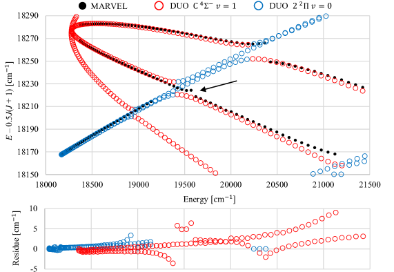
Figure 6: State interaction of $\mathrm{C}\,^{4}\Sigma^{-},v=1$ and $\mathrm{2}\,^{2}\Pi,v=0$. The black dots in the top panel are the rovibronic energy levels obtained from MARVEL analysis [36] while the circles are the fitting results of Duo. The rotational constant of $\mathrm{2}\,^{2}\Pi,v=0$ in derived from our model is consistent with that of the recently assigned results (see the blue circles in the top panel). However, it crossing point with the $F_{2}$ series of $\mathrm{C}\,^{4}\Sigma^{-},v=1$ is inconsistent with experimental values (see the area pointed by the black arrow). The bottom panel shows the fitting residues.

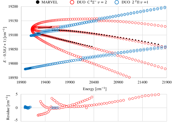
Figure 7: State interaction of $\mathrm{C}\,^{4}\Sigma^{-},v=2$ and $\mathrm{2}\,^{2}\Pi,v=1$. The black dots in the top panel are the rovibronic energy levels obtained from MARVEL analysis [36] while the circles are the fitting results of Duo. The bottom panel shows the fitting residues.

The $v=0$ levels of $\mathrm{C}\,^{4}\Sigma^{-}$ do not interact with the $\mathrm{2}\,^{2}\Pi$ state. Thus, the diagonal spin-rotation coupling term in Table 4 was determined by the states with the $v=0$ levels. Nevertheless, there are still systematic errors as shown in Fig. 8. The $J$-dependent fitting residues of high-$J$ levels should be attributed to $\mathrm{C}\,^{4}\Sigma^{-}-\mathrm{1}\,^{2}\Pi$ interaction, although more experimental data are needed to verify this.

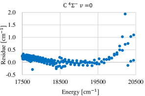
Figure 8: Fitting residues of $\mathrm{C}\,^{4}\Sigma^{-},v=0$.

3.3 Fitting quality

The root-mean-square error ($\mathrm{RMSE}$) of the fitting residues for each electronic state is calculated as

$$\mathrm{RMSE}=\sqrt{\frac{1}{N}\sum_{i=1}^{N}e_{i}}\,,$$ (8)

where $e_{i}$ is the fitting error of the $i$-th energy level and $N$ is the number of rovibronic states included. The values of $\mathrm{RMSE}$ are listed in Table 8.

Table 8: RMSE and maximum absolute error of each state in cm^-1.

State	${v}$	RMSE	Max absolute error
$\mathrm{X}\,^{4}\Sigma^{-}$	0	0.0777	0.2404
	1	0.0168	0.2369
	2	0.0651	0.1884
$\mathrm{A}^{\prime}\,{}^{4}\Phi$	0	0.2241	0.5760
	1	1.3634	2.8620
	2	0.206	0.5821
$\mathrm{A}\,^{4}\Pi$	0	0.1766	0.5131
$\mathrm{D}\,^{4}\Delta$	0	0.1893	0.9044
	1	2.3556	4.2883
$\mathrm{1}\,^{2}\Delta$	0	0.2675	1.4664
	1	0.2107	0.7573
$\mathrm{1}\,^{2}\Phi$	0	0.0507	0.1362
$\mathrm{1}\,^{2}\Pi$	0	0.0363	0.1380
	1	0.1145	0.3368
	2	0.0696	0.1217
	3	0.0603	0.1372
$\mathrm{B}\,^{4}\Pi-\mathrm{1}\,^{2}\Sigma^{+}$		0.4234	1.2228
$\mathrm{C}\,^{4}\Sigma^{-}$	0	0.2949	1.9393
$\mathrm{C}\,^{4}\Sigma^{-}-\mathrm{2}\,^{2}\Pi$		1.4829	9.0335

The VOMYT model was refined using Model Hamiltonian, combination difference energy levels and transition frequencies [19]. As most of the transitions connect to the ground electronic state, VOMYT has a reasonable representation of $\mathrm{X}\,^{4}\Sigma^{-}$. However, its vibrational structure was still not accurately determined as shown in Fig. 9. There is an obvious offset of the $v=2$ energy levels, which is likely to be significantly worse for higher vibrationally excited states. The $\mathrm{RMSE}$ value for the VOMYT model is $0.3015\text{\,}{\mathrm{cm}}^{-1}$, about four times worse than ours.

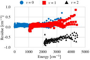
Figure 9: Energy errors for the $\mathrm{X}\,^{4}\Sigma^{-}$ state as given by the VOMYT model.

The rotational constants of all states in our model are around $0.5\text{\,}{\mathrm{cm}}^{-1}$ and the rotational energy gaps are estimated as

$$\Delta E=0.5(J+2)(J+1)-0.5(J+1)J=J+1\quad${\mathrm{cm}}^{-1}$.$$ (9)

Thus, our model achieves sufficient accuracy to make rotational assignments. The coupling curves can be further refined once revised or extended data is available.

4 Conclusions

We propose an empirical spectroscopic model for 6 quartet and 5 doublet states of VO. The most recent MARVEL analysis of VO [36] generates accurate energy term values for this molecule, which makes it possible to achieve experimental accuracy for some vibronic levels compared with VOMYT [19]. The interactions of $\mathrm{B}\,^{4}\Pi-\mathrm{1}\,^{2}\Sigma^{+}$ and $\mathrm{C}\,^{4}\Sigma^{-}-\mathrm{1}\,^{2}\Pi$ are analyzed by introducing the off-diagonal spin-orbit couplings between them.

While our model represents a significant advance on what is currently available, there remains two outstanding issues. The first is the treatment of resonance interactions which is discussed extensively above. Given that state-of-the-art ab initio calculations on systems with a transition metal atom are not capable of even approaching the accuracy required for high resolution studies, improving our model will require further experimental input.

The second issue is the hyperfine structure. The main isotope of vanadium, ⁵¹V, has a nuclear spin $I=7/2$ which is known to lead to pronounced hyperfine effects in the spectrum of VO [25, 30, 34]. We have started to address this issue by extending our nuclear motion program Duo to explicitly include hyperfine effects [46] within its variational model. We have also built a hyperfine-resolved spectroscopic model for the ground $\mathrm{X}\,^{4}\Sigma^{-}$ state of ⁵¹V¹⁶O [2]. We are working on extending the model to other electronic states of VO to give a spectroscopically-accurate, hyperfine-resolved model of the molecule. Given the limited experimental hyperfine-resolved data available for VO, particularly for spectra involving excited vibrational states, further experimental input into this problem would be particularly welcome.

Data Availability

The open access programs ExoCross and Duo are available from github.com/exomol. The Duo input file used in this work is given as supplementary material; our potential energy and coupling curves are included as part of this input file.

References

- [1] A. J. Merer, Spectroscopy of the diatomic 3d transition-metal oxides, Ann. Rev. Phys. Chem. 40 (1989) 407–438. doi:10.1146/annurev.pc.40.100189.002203.
- [2] Q. Qu, S. N. Yurchenko, J. Tennyson, A variational model for the hyperfine resolved spectrum of VO in its ground electronic state, J. Chem. Phys. (2022). doi:10.1063/5.0105965.
- [3] P. F. Bernath, Molecular astronomy of cool stars and sub-stellar objects, Int. Rev. Phys. Chem. 28 (2009) 681–709. doi:10.1080/01442350903292442.
- [4] J. J. Fortney, K. Lodders, M. S. Marley, R. S. Freedman, A Unified Theory for the Atmospheres of the Hot and Very Hot Jupiters: Two Classes of Irradiated Atmospheres, Astrophys. J. 678 (2008) 1419–1435. doi:10.1086/528370.
- [5] N. Madhusudhan, S. Seager, On the inference of thermal inversions in hot Jupiter atmospheres, Astrophys. J. 725 (2010) 261. doi:10.1088/0004-637X/725/1/261.
- [6] R. Tylenda, T. Kamiński, M. Schmidt, R. Kurtev, T. Tomov, High-resolution optical spectroscopy of V838 Monocerotis in 2009, Astron. Astrophys. 532 (2011) A138. doi:10.1051/0004-6361/201116858.
- [7] P. Sriramachandran, S. P. Bagare, N. Rajamanickam, K. Balachandrakumar, Presence of LaO, ScO and VO Molecular Lines in Sunspot Umbral Spectra, Sol. Phys. 252 (2008) 267–281. doi:10.1007/s11207-008-9261-1.
- [8] T. M. Evans, D. K. Sing, H. R. Wakeford, N. Nikolov, G. E. Ballester, B. Drummond, T. Kataria, N. P. Gibson, D. S. Amundsen, J. Spake, Detection of H2O and evidence for tio/vo in an ultra-hot exoplanet atmosphere, Astrophys. J. 822 (2016) L4. doi:10.3847/2041-8205/822/1/l4.
- [9] J. D. Turner, R. M. Leiter, L. I. Biddle, K. A. Pearson, K. K. Hardegree-Ullman, R. M. Thompson, J. K. Teske, I. T. Cates, K. L. Cook, M. P. Berube, M. N. Nieberding, C. K. Jones, B. Raphael, S. Wallace, Z. T. Watson, R. E. Johnson, Investigating the physical properties of transiting hot Jupiters with the 1.5-m Kuiper Telescope, Mon. Not. R. Astron. Soc. 472 (2017) 3871–3886. doi:10.1093/mnras/stx2221.
- [10] E. Palle, G. Chen, J. Prieto-Arranz, G. Nowak, F. Murgas, L. Nortmann, D. Pollacco, K. Lam, P. Montanes-Rodriguez, H. Parviainen, N. Casasayas-Barris, Feature-rich transmission spectrum for WASP-127b Cloud-free skies for the puffiest known super-Neptune?, Astron. Astrophys. 602 (2017). doi:{10.1051/0004-6361/201731018}.
- [11] A. Tsiaras, I. P. Waldmann, T. Zingales, M. Rocchetto, G. Morello, M. Damiano, K. Karpouzas, G. Tinetti, L. K. McKemmish, J. Tennyson, S. N. Yurchenko, A population study of gaseous exoplanets, Astron. J. 155 (2018) 156. doi:10.3847/1538-3881/aaaf75.
- [12] J. M. Goyal, N. Mayne, B. Drummond, D. K. Sing, E. Hebrard, N. Lewis, P. Tremblin, M. W. Phillips, T. Mikal-Evans, H. R. Wakeford, A library of self-consistent simulated exoplanet atmospheres, Mon. Not. R. Astron. Soc. 498 (2020) 4680–4704. doi:10.1093/mnras/staa2300.
- [13] N. K. Lewis, H. R. Wakeford, R. J. MacDonald, J. M. Goyal, D. K. Sing, J. Barstow, D. Powell, T. Kataria, I. Mishra, M. S. Marley, N. E. Batalha, J. I. Moses, P. Gao, T. J. Wilson, K. L. Chubb, T. Mikal-Evans, N. Nikolov, N. Pirzkal, J. J. Spake, K. B. Stevenson, J. Valenti, X. Zhang, Into the UV: The Atmosphere of the Hot Jupiter HAT-P-41b Revealed, Astrophys. J. Lett. 902 (2020) L19. doi:{10.3847/2041-8213/abb77f}.
- [14] Q. Changeat, B. Edwards, The hubble WFC3 emission spectrum of the extremely hot jupiter KELT-9b, Astrophys. J. Lett. 907 (2021) L22. doi:10.3847/2041-8213/abd84f.
- [15] E. Miliordos, A. Mavridis, Electronic structure of vanadium oxide. Neutral and charged species, VO0,±, J. Phys. Chem. A 111 (2007) 1953–1965. doi:10.1021/jp067451b.
- [16] T. Rivlin, L. K. McKemmish, K. E. Spinlove, J. Tennyson, Low-temperature scattering with the R-matrix method: from nuclear scattering to atom-atom scattering and beyond, SciPost Phys. Proc. (2020).
- [17] L. K. McKemmish, S. N. Yurchenko, J. Tennyson, Ab initio calculations to support accurate modelling of the rovibronic spectroscopy calculations of vanadium monoxide (VO), Mol. Phys. 114 (2016) 3232–3248. doi:10.1080/00268976.2016.1225994.
- [18] T. Jiang, Y. Chen, N. A. Bogdanov, E. Wang, A. Alavi, J. Chen, A full configuration interaction quantum Monte Carlo study of ScO, TiO, and VO molecules, J. Chem. Phys. (2021) 164302doi:10.1063/5.0046464.
- [19] L. K. McKemmish, S. N. Yurchenko, J. Tennyson, ExoMol Molecular linelists – XVIII. The spectrum of Vanadium Oxide, Mon. Not. R. Astron. Soc. 463 (2016) 771–793. doi:10.1093/mnras/stw1969.
- [20] J. Tennyson, S. N. Yurchenko, ExoMol: molecular line lists for exoplanet and other atmospheres, Mon. Not. R. Astron. Soc. 425 (2012) 21–33. doi:10.1111/j.1365-2966.2012.21440.x.
- [21] J. Tennyson, S. N. Yurchenko, A. F. Al-Refaie, V. H. J. Clark, K. L. Chubb, E. K. Conway, A. Dewan, M. N. Gorman, C. Hill, A. E. Lynas-Gray, T. Mellor, L. K. McKemmish, A. Owens, O. L. Polyansky, M. Semenov, W. Somogyi, G. Tinetti, A. Upadhyay, I. Waldmann, Y. Wang, S. Wright, O. P. Yurchenko, The 2020 release of the ExoMol database: molecular line lists for exoplanet and other hot atmospheres, J. Quant. Spectrosc. Radiat. Transf. 255 (2020) 107228. doi:10.1016/j.jqsrt.2020.107228.
- [22] S. de Regt, A. Y. Kesseli, I. A. G. Snellen, S. R. Merritt, K. L. Chubb, A quantitative assessment of the VO line list: Inaccuracies hamper high-resolution VO detections in exoplanet atmospheres, Astron. Astrophys. 661 (2022) A109. doi:10.1051/0004-6361/202142683.
- [23] A. Lagerqvist, L. E. Selin, Rotationsanalyse der sichtbaren Vanadiumoxydbanden, Arkiv for Fysik 12 (1957) 553–568.
- [24] W. H. Hocking, A. J. Merer, D. J. Milton, Resolved hyperfine structure in the C–X electronic transition of VO. An internal hyperfine perturbation in the C state, Can. J. Phys. 59 (1981) 266–270. doi:10.1139/p81-035.
- [25] A. S.-C. Cheung, R. C. Hansen, A. J. Merer, Laser spectroscopy of VO: Analysis of the rotational and hyperfine structure of the C –X (0, 0) band, J. Mol. Spectrosc. 91 (1982) 165–208. doi:10.1016/0022-2852(82)90039-X.
- [26] A. S.-C. Cheung, A. W. Taylor, A. J. Merer, Fourier transform spectroscopy of VO: Rotational structure in the A –X system near 10 500 Å, J. Mol. Spectrosc. 92 (1982) 391–409. doi:10.1016/0022-2852(82)90110-2.
- [27] A. J. Merer, G. Huang, A. S.-C. Cheung, A. W. Taylor, New quartet and doublet electronic transitions in the near-infrared emission spectrum of VO, J. Mol. Spectrosc. 125 (1987) 465–503. doi:10.1016/0022-2852(87)90110-X.
- [28] R. D. Suenram, G. T. Fraser, F. J. Lovas, C. W. Gillies, Microwave spectra and electric dipole moments of X VO and NbO, J. Mol. Spectrosc. 148 (1991) 114–122. doi:10.1016/0022-2852(91)90040-H.
- [29] A. S.-C. Cheung, P. G. Hajigeorgiou, G. Huang, S. Z. Huang, A. J. Merer, Rotational Structure and Perturbations in the B –X (1, 0) Band of VO, J. Mol. Spectrosc. 163 (1994) 443–458. doi:10.1006/jmsp.1994.1039.
- [30] A. G. Adam, M. Barnes, B. Berno, R. D. Bower, A. J. Merer, Rotational and Hyperfine Structure in the B –X (0,0) Band of VO at 7900 Å: Perturbations by the a , v = 2 Level, J. Mol. Spectrosc. 170 (1995) 94–130. doi:10.1006/jmsp.1995.1059.
- [31] L. Karlsson, B. Lindgren, C. Lundevall, U. Sassenberg, Lifetime Measurements of the A , B , and C States of VO, J. Mol. Spectrosc. 181 (1997) 274–278. doi:10.1006/jmsp.1996.7173.
- [32] R. S. Ram, P. F. Bernath, S. P. Davis, A. J. Merer, Fourier Transform Emission Spectroscopy of a New –1 System of VO, J. Mol. Spectrosc. 211 (2002) 279–283. doi:10.1006/jmsp.2001.8510.
- [33] R. S. Ram, P. F. Bernath, Emission spectroscopy of a new –1 system of VO, J. Mol. Spectrosc. 229 (2005) 57–62. doi:10.1016/j.jms.2004.08.014.
- [34] M. A. Flory, L. M. Ziurys, Submillimeter-wave spectroscopy of VN (X ) and VO (X ): A study of the hyperfine interactions, J. Mol. Spectrosc. 247 (2008) 76–84. doi:10.1016/j.jms.2007.09.007.
- [35] W. S. Hopkins, S. M. Hamilton, S. R. Mackenzie, The electronic spectrum of vanadium monoxide across the visible: New bands and new insight, J. Chem. Phys. 130 (2009) 144308. doi:10.1063/1.3104844.
- [36] C. A. Bowesman, H. Akbari, S. Hopkins, S. N. Yurchenko, J. Tennyson, Fine and hyperfine resolved empirical energy levels for VO, J. Quant. Spectrosc. Radiat. Transf. 289 (2022) 108295. doi:10.1016/j.jqsrt.2022.108295.
- [37] L. K. McKemmish, T. Masseron, J. Hoeijmakers, V. V. Pérez-Mesa, S. L. Grimm, S. N. Yurchenko, J. Tennyson, ExoMol Molecular line lists – XXXIII. The spectrum of Titanium Oxide, Mon. Not. R. Astron. Soc. 488 (2019) 2836–2854. doi:10.1093/mnras/stz1818.
- [38] C. A. Bowesman, M. Shuai, S. N. Yurchenko, J. Tennyson, A high resolution line list for AlO, Mon. Not. R. Astron. Soc. 508 (2021) 3181–3193. doi:10.1093/mnras/stab2525.
- [39] S. N. Yurchenko, J. Tennyson, A.-M. Syme, A. Y. Adam, V. H. J. Clark, B. Cooper, C. P. Dobney, S. T. E. Donnelly, M. N. Gorman, A. E. Lynas-Gray, T. Meltzer, A. Owens, Q. Qu, M. Semenov, W. Somogyi, A. Upadhyay, S. Wright, J. C. Zapata Trujillo, ExoMol line lists – XLIV. IR and UV line list for silicon monoxide (28Si16O), Mon. Not. R. Astron. Soc. 510 (2022) 903–919. doi:10.1093/mnras/stab3267.
- [40] M. Semenov, J. Tennyson, S. N. Yurchenko, ExoMol line lists – XLVI: Empirical rovibronic spectra of silicon mononitrate (SiN) covering 6 lowest electronic states and 4 isotopologues, Phys. Chem. Chem. Phys. 516 (2022) 1158–1169. doi:10.1093/mnras/stac2004.
- [41] C. M. Western, PGOPHER: A program for simulating rotational, vibrational and electronic spectra , J. Quant. Spectrosc. Radiat. Transf. 186 (2017) 221–242. doi:10.1016/j.jqsrt.2016.04.010.
- [42] T. Furtenbacher, A. G. Császár, J. Tennyson, MARVEL: measured active rotational-vibrational energy levels, J. Mol. Spectrosc. 245 (2007) 115–125. doi:10.1016/j.jms.2007.07.005.
- [43] S. N. Yurchenko, L. Lodi, J. Tennyson, A. V. Stolyarov, Duo: a general program for calculating spectra of diatomic molecules, Comput. Phys. Commun. 202 (2016) 262–275. doi:10.1016/j.cpc.2015.12.021.
- [44] E. G. Lee, J. Y. Seto, T. Hirao, P. F. Bernath, R. J. Le Roy, FTIR emission spectra, molecular constants, and potential curve of ground state GeO, J. Mol. Spectrosc. 194 (1999) 197–202. doi:10.1006/jmsp.1998.7789.
- [45] J. M. Brown, A. J. Merer, Lambda-type doubling parameters for molecules in -electronic states of triplet and higher multiplicity, J. Mol. Spectrosc. 74 (1979) 488–494. doi:10.1016/0022-2852(79)90172-3.
- [46] Q. Qu, S. N. Yurchenko, J. Tennyson, Hyperfine-resolved variational nuclear motion spectra of diatomic molecules, J. Chem. Theory Comput. 18 (2022) 1808–1820. doi:10.1021/acs.jctc.1c01244.