Tidal disruption of stellar clusters and their remnants’ spatial distribution near the galactic center

Abstract

The accretion of massive star clusters via dynamical friction has previously been established to be a likely scenario for the build up of nuclear stellar clusters (NSCs). A remaining issue is whether strong external tidal perturbation may lead to the severe disruption of loosely-bound clusters well before they sink deeply into the center of their host galaxies. We carry out a series of $N$-body simulations and verify our early idealized analytic models. We show if the density profile of the host galaxies can be described by a power-law distribution with an index, $\alpha<1$, the cluster would be compressed in the radial direction by the external galactic tidal field. In contrast, the galactic tidal perturbation is disruptive in regions with a steep, $\alpha>1$, density fall-off or in the very center where gravity is dominated by the point-mass potential of super-massive black holes (SMBHs). This sufficient criterion supplements the conventional necessary Roche-lobe-filling condition in determining the preservation versus disintegration of satellite stellar systems. We simulate the disruption of stellar clusters which venture on nearly-circular, modestly- or highly-eccentric orbits into the center of galaxies with a range of background density profiles and SMBHs. We obtain the spatial distribution of the stellar-cluster remnants. We apply these results to the NSC within a few parsecs from SMBH Sgr A^∗ at the Galactic Center. Recent observations indicate the coexistence of two populations of stars with distinctively separate ages and metallicities. We verify that the subsolar-metalicity population can be the debris of disrupted stellar clusters.

1 Introduction

The widely adopted $\Lambda$CDM model of galaxy formation is based on the assumption that relative dense early-generation dwarf galaxies form, merge, and assemble into larger entities(White & Rees, 1978; Blumenthal et al., 1984). A prediction of this hypothesis is the preservation of ubiquitous satellites which survived the tidal disruption during their dynamical evolution(Navarro et al., 1995). Recent discoveries of many debris stellar streams provide supporting evidences for this scenario (Myeong et al., 2018; Helmi et al., 2018). If their dense nuclei with sufficient mass ($\gtrsim 3\times 10^{7}M_{\odot}$) can be preserved, they may converge towards the centers of amalgamated stellar systems and their merged halo(Fall & Rees, 1977).

Nuclear stellar clusters are also commonly found in galaxies (see the extensive contributions by many investigators cited in two annual review articles by Kormendy & Ho (2013) and Neumayer et al. (2020)). A natural extrapolation is that these clusters were formed in the inner ($<$ a few kpc) region and migrated to the center of their host galaxies under the action of dynamical friction (Tremaine et al., 1975; Tremaine, 1976). Near the central region of the Galaxy, there are several stellar clusters including Archies and Quintuplet (Nagata et al., 1995; Cotera et al., 1996). Within a few pc from the Sgr A^∗ supermassive black hole (SMBH) (Genzel et al., 1997; Ghez et al., 1998), there is a nuclear cluster with $\sim 1-2\times 10^{7}$ mature stars (Do et al., 2009; Schödel et al., 2014) in addition to the $\sim 10^{2}$ bright young massive S and disk stars (Ghez et al., 2003). The nuclear-cluster stars show substructure in kinematics, heavy element abundance, and stellar ages (Feldmeier et al., 2014; Do et al., 2020).

In addition to the Occam’s-razor in-situ formation scenario for the origin of nuclear clusters(Loose et al., 1982; Agarwal & Milosavljević, 2011), it has been widely suggested that they contain stars formed in progenitor clusters beyond a few Kpc, endured orbital decay under the action of dynamical friction (e.g., Capuzzo-Dolcetta, 1993; Oh & Lin, 2000; Lotz et al., 2001; Capuzzo-Dolcetta & Mastrobuono-Battisti, 2009; Antonini, 2013; Feldmeier et al., 2014; Gnedin et al., 2014; Arca-Sedda & Capuzzo-Dolcetta, 2014). Several series of N-body simulations provided quantitative supports for this hypothesis (e.g., Oh & Lin, 2000; Capuzzo-Dolcetta & Miocchi, 2008; Antonini et al., 2012; Perets & Mastrobuono-Battisti, 2014; Arca-Sedda et al., 2015a, 2016; Arca-Sedda & Capuzzo-Dolcetta, 2017a, b; Arca-Sedda & Gualandris, 2018; Tsatsi et al., 2017; Arca Sedda et al., 2020). They have already demonstrated this scenario can account for the origin of common-rotation and diverse-abundance properties among subgroups of nuclear cluster stars (e.g., Feldmeier et al., 2014; Tsatsi et al., 2017; Fahrion et al., 2020; Arca Sedda et al., 2020).

Nevertheless, there is a remaining issue of how close to the Galactic center can the clusters deliver a substantial fraction of their constituent stars. Loosely bond stellar clusters and satellite dwarf galaxies have a tendency to undergo tidal disruptions within a conventionally-defined “tidal disruption distance” $R_{\rm d}$ at Galactocentric distances of a fraction to a few kpc (Fall & Rees, 1977; Oh & Lin, 1992; Oh et al., 1995; Fellhauer & Lin, 2007). The central objective of this paper is to examine this ongoing dispersal issue based on the assumption that the parent clusters can make their way towards the Galactic center.

The Galactic potential has a complex radial dependence which has been approximated as a composite of several components, including the bulge, disk, halo (Gnedin et al., 2005; Widrow & Dubinski, 2005), and the SMBH. Moreover satellite galaxies and stellar clusters have diverse internal structure(Baumgardt et al., 2019; Baumgardt & Vasiliev, 2021). Many investigators have studied how star clusters can survive in the effect of tidal disruption during their arduous journey through different regions and at various evolutionary stages of their host galaxies. In some cases, they combine semi-analytic treatments to model star cluster dynamics with actual galaxy models from magneto hydro-dynamical cosmological simulations(e.g. Gnedin et al., 2014; Longmore et al., 2014; Kruijssen et al., 2014, 2015; Pfeffer et al., 2018; Choksi et al., 2018; Li et al., 2018). Near the Galactic center, if the mass of SMBH significantly exceeds the mass of infalling GCs, they would be completely disrupted before they reach a few pc from the SMBH (Arca-Sedda et al., 2015a). This issue is directly relevant to the dynamical structure at the very center of NSCs and perhaps the formation of SMBHs in galaxies. Fittings of the observed surface brightness with the Sersic (1968) model show a wide variation in the light and mass distribution among different galaxy populations, including those with or without nuclear clusters (Böker et al., 2002; Misgeld & Hilker, 2011; Kormendy & Ho, 2013). The poorly-resolved surface-brightness and the inferred mass-density distribution within the central few pc from any SMBH at the galactic centers also vary considerably. A complementary study on the disruption and survivability of stellar clusters in a diverse set of galactic potential is warranted.

Motivated by this generic problem, we carried out an investigation on the secular evolution of stellar clusters in a general galactic tidal field (Ivanov & Lin, 2020). Based on a rigorously-constructed, idealized formalism (Mitchell & Heggie, 2007), we analytically showed that the tidal field of a background potential associated with a sufficiently flat density distribution can lead to compression rather than disruption. We also showed that even the most vulnerable homogeneous star cluster (in contrast with the more tightly-bound models with dense cores or intermediate-mass black holes, IMBHs) can meander to distances much smaller than the conventional $R_{\rm d}$ without disruption, thus potentially contribute to the accumulation of stars in the NSCs. Although these analytic approximations provide a quantitative illustration on the critical conditions, they are derived for clusters with idealized, uniform density distribution. In order to verify and generalize the results of our previous analytic approximation, we carry out a series of numerical N-body simulations with more a general Michie (1963)-King (1966) model for the initial stellar density distributions. In §2, we briefly describe the numerical method, initial and boundary condition. In §3, we simulate the evolution of a cluster’s internal density distribution. For initial conditions, we chose the cluster’s density to be homogeneous or follows King models with various concentration parameter. The cluster is initially on a circular orbit around galactic potential associated with various mass distribution, including a point mass to represent a SMBH. We consider, in §4 the survival of clusters with gradually decaying (nearly circular) and plunging (highly eccentric) orbits. In §5, we summarize the results of our numerical simulation and discuss their implications including the possibilities that in-situ star formation may also be a major contribution to the NSC build-up (e.g. Antonini et al., 2015; Portegies Zwart et al., 2002) and the Milky-Way NSC may be built-up by both accreted massive star clusters and in-situ star formation, as shown from Chemo-dynamical analysis by Do et al. (2020).

2 Numerical simulations

We aim to investigate whether a star cluster can survive the tidal perturbation induced by the galactic potential. If the cluster is severely or completely disrupted during its passage through the conventional tidal-disruption radius $R_{\mathrm{d}}$, its tidal debris would form a ring along that radius and there would not be any subsequent mechanism that can efficiently bring the detached stars closer to the galactic center. But if the cluster is tidally compressed, it would survive and migrate well inside $R_{\mathrm{d}}$, as suggested by Ivanov & Lin (2020). To verify whether debris stars can reach the SMBH proximity, we carry out a series of N-body simulations, to demonstrate the effects of tidal compression and disruption, depending on the density profiles of the star clusters, the potentials of the galaxies, and the orbits of the clusters.

2.1 N-body code

In this work, we use the $N$-body code petar (Wang et al., 2020a) to perform the numerical simulations of the star clusters. The code is designed for simulating dense stellar systems where close encounters and dynamics of binaries are important. The particle-tree and particle-particle methods (Oshino et al., 2011), embedded in the framework for developing parallel particle simulation codes (fdps), are used to achieve a high computing performance (Iwasawa et al., 2016, 2020). The slow-down algorithmic regularization method (SDAR; Wang et al., 2020b) is designed and implemented to accurately follow the orbital motions of binaries, hyperbolic encounters and hierarchical few-body systems. The tidal force from the Galactic potential is calculated with the galpy code (Bovy, 2015).

2.2 Star cluster model

In our $N$-body simulation, we neglect stellar evolution and non-uniform mass function, i.e. all stars are assigned with the same mass and lifespan longer than the computational time span. In principle, the stellar-wind mass loss and the phase-space segregation of multiple-mass components can affect the dynamical evolution of star clusters and subsequently influence the survival of star clusters (Portegies Zwart et al., 2002). In general, these physical processes cannot be ignored. But the mixture of them in one set of simulations would introduce some difficulties in disentangling their relative impacts. For the purpose of this investigation, we adopt an idealized approximation to keep the $N$-body models relatively simple.

The total initial number of stars in most $N$-body models are fixed to be 1000. At the beginning of each simulation, the system is constructed to be in a virial equilibrium. This model does not fully represent a genuine globular cluster in nature, which typically contains million evolving stars with a range of masses. But it is time-consuming to carry out such comprehensive simulations. In this investigation, we simulate many models with a wide range of other parameters, including the clusters’ internal and galaxies’ external mass distribution as well as clusters’ orbital evolution (Table 2). With limited computational resources, it is practical to simplify and speed up the simulations with cluster models more sensitive to the tidal effect and neglect less-dominant relaxation effects. Nevertheless, we compare the results of tidal-response models with NoTide calibration models and verify that our results are not significantly affected by spurious internal two-body relaxation effects during the simulated time intervals. Our analysis does not lose generality, since the external (Galactic) tidal effect is always present, regardless of the clusters’ mass, albeit their evolutionary time scale may vary.

We adopt two types of initial-density profile for the clusters: an idealized spherical-symmetric, homogeneous mass-density distributionMitchell & Heggie (2007) and a series of Michie (1963)- King (1966) models. The former setup is the simplest model where the tidal effect can be described and analyzed with an analytic approach. These clusters are also most vulnerable to external perturbation. We adopt it to validate the prediction of Ivanov & Lin (2020). But this idealized homogeneous model is unrealistic with respect to the observed star clusters. Thus, we carry out additional simulations with the Michie (1963)-King (1966) profile, which is commonly adopted to describe the observed surface-brightness distribution of globular clusters with a dense core and tidal cutoff of the outer region.

Most of our models contain $10^{3}$ stars which is well below the star counts inside typical globular clusters in nature. In order to build-up statistical significance with such small number of cluster stars, we usually need to carry out many simulations with the same initial condition but different random seeds to generate the positions and velocities of stars. We obtain some average trends among these models to represent the mean expectation values and to smooth out any stochastic scatter. In this work, we only prepare one initial model (one random seed) for each type of density profile. With this approach, when we choose a certain density profile and compare the effect from different Galactic potentials, we are ensured to compare the simulations with the identical initial positions and velocities of stars. This prescription can also reduce the impact from small-number stochastic scatter. With a series of statistical tests (Fig. 5), we verify that this approach is sufficient in our analysis, since the tidal effect is very pronounced.

2.2.1 Units and scaling

To describe the dynamical evolution of star clusters, we calculate two important timescales: the crossing time ($T_{\mathrm{cr}}$) and the two-body relaxation time ($T_{\mathrm{rh}}$). The crossing time $T_{\mathrm{cr}}$ is defined to be

$$T_{\mathrm{cr}}\equiv\sqrt{\frac{r_{\mathrm{h}}^{3}}{GM_{\mathrm{sc}}}},$$ (1)

where $r_{\mathrm{h}}$ is the half-mass radius of a cluster. For equal-mass system, $T_{\mathrm{rh}}$ can be described as (Spitzer, 1987)

$$T_{\mathrm{rh}}\approx 0.138\frac{N^{1/2}r_{\mathrm{h}}^{3/2}}{m^{1/2}G^{1/2}\ln\Lambda},$$ (2)

where $\Lambda=0.4N$ and $m$ is the mass of star. We use the initial $T_{\mathrm{rh}}$ ($T_{\mathrm{rh0}}$) as the time unit and the cluster’s initial cut-off (tidal) radius $r_{\mathrm{t}}$ (Eq. 3) as the radial unit. Thus, the result can be scaled to arbitrary systems with a free choice of $M_{\mathrm{sc}}$ and $r_{\mathrm{h}}$, and it can also represent star clusters with different $N$ but the same $T_{\mathrm{rh}}$.

2.2.2 Idealized clusters with spherically symmetric homogeneous density profile

For a star cluster moving in a circular orbit, the conventional tidal radius of the cluster can be approximated as

$$r_{\mathrm{t}}(R)\approx\left[\frac{M_{\mathrm{sc}}}{3M_{\mathrm{g}}(R)}\right]^{\frac{1}{3}}R$$ (3)

where $M_{\mathrm{sc}}$ is the total mass of the cluster. The density profile of a homogeneous star cluster can be described as

$$\rho_{\mathrm{sc}}(r)=\begin{cases}\frac{4M_{\mathrm{sc}}}{3\pi r_{\rm cut}^{3}}&\text{for}~{}r<r_{\mathrm{cut}}\\ 0&\text{otherwise}\end{cases}$$ (4)

where $r$ is the distance to the center of a cluster (§3.1.1), and $r_{\mathrm{cut}}$ is the cut-off radius of the cluster. The velocity distribution of stars follows the Maxwell distribution with a distance dependent scaling factor:

$$f(v,r)=\sqrt{\frac{2GM_{\mathrm{sc}}}{3\pi}}v^{2}\exp{\left(\frac{-v^{2}}{2}\right)}\frac{r}{r_{\mathrm{cut}}}.$$ (5)

We place the clusters at $R=R_{\mathrm{g}}$ from the center of the galactic potential where $R_{\mathrm{g}}$ is a reference distance (also see Eq. 6) and the clusters’ $r_{\mathrm{cut}}$ is set to be $r_{\mathrm{t}}$. This location corresponds to the conventional galacto-centric distance where the clusters are assumed to be on the verge of tidal disruption.

2.2.3 The Michie-King model of stellar clusters

The Michie (1963)-King (1966) model describes a stellar system with a non-singular isothermal sphere. There are two free parameters: $r_{\mathrm{cut}}$ and the concentration parameter $W_{0}$, which indicates the ratio between $r_{\mathrm{cut}}$ and the core radius ($r_{\mathrm{c}}$). In observational interpretation, $r_{\mathrm{cut}}$ is often considered to be $r_{\mathrm{t}}$ . We also adopt this convention in most models presented here such that $R_{\mathrm{g}}$ is the conventional galacto-centric distance where the clusters are assumed to be on the verge of tidal disruption and the conventional, necessary, Roche-lobe-filling condition for tidal disruption is $R\leq R_{\mathrm{g}}$. To verify whether the computational results are independent of the initial conditions (§2.3.2), $r_{\mathrm{t}}$ and $r_{\rm cut}$ are chosen separately in some test models. A part of our models adopt three Michie-King profiles with $W_{0}=2,6$ and $8$ (hereafter named as W2, W6 and W8), respectively (§3.1.2). The W2 profile has a low concentration, the W6 profile is similar to the Plummer (1911) profile. Due to the low number of stars, the W8 profile does not show significant difference of central density referring to that of W6. Thus, these three are sufficient to represent a wide range of density distribution.

2.3 Galactic potential

Ivanov & Lin (2020) suggest that for a static power-law spherically symmetric galactic potential with a small power index ($\alpha$), a star cluster with the homogeneous density profile can suffer tidal compression instead of tidal disruption. Consequently, the cluster can migrate to the inner region of the galactic center. Firstly, we carry out $N$-body simulations with this one-component static potential for different values of $\alpha$, in order to validate the theoretical prediction. This potential represents that of the galactic bulge. We place star clusters with different density profiles on a circular orbit to investigate their morphological evolution. We determine the critical value of $\alpha$ which represents the boundary between tidal disruption and compression.

For the next step, we introduce a point-mass potential superimposed onto the power-law potential to represent galaxies with central SMBHs. We choose the power-law potential with $\alpha=0.5$ which, in the absence of the SMBH, provides the effect of tidal compression. The additional SMBH provides the counter-effect of tidal disruption. We vary the mass ratio between these two components and find the boundary between these competing effects.

Previous investigations have provided well-established evidences that clusters migrate inwards under the action of dynamical friction. In their presence at the center of the galaxy, SMBHs’ tidal influence intensify as a stellar cluster undergoes orbital decay towards the galactic center. To reproduce the migration of clusters, we artificially increase the total mass of the potential instead of implementing dynamical friction in the $N$-body code. In this prescription, the cluster smoothly sinks into the center of the galaxy with an in-spiraling orbit (§A). We investigate whether the tidal compression can help the cluster to survive inside the conventional $R_{\mathrm{d}}$. We also investigate the survival of star clusters with modestly and highly eccentric orbits, where they approach the galactic center at their perigee much faster than any in-spiraling migration due to dynamical friction.

2.3.1 One-component static background potential

By defining $R$ as the distance to the galactic center, the density profile for the static power-law spherically-symmetric potential can be written as

$$\rho_{\mathrm{g}}(R)=\rho_{\mathrm{g0}}\left(\frac{R_{\mathrm{g}}}{R}\right)^{\alpha},$$ (6)

where $0<\alpha\leq 3$, $R_{\mathrm{g}}$ is a reference distance, and $\rho_{\mathrm{g0}}$ is the reference density defined at $R=R_{\mathrm{g}}$. The corresponding enclosed mass of the galaxy at $R$ is

$$M_{\mathrm{g}}(R)=4\pi\rho_{\mathrm{g0}}R_{\mathrm{g}}^{\alpha}\begin{cases}\frac{R^{3-\alpha}}{3-\alpha}&\text{for}~{}\alpha\neq 3\\ \ln(R)&\text{for}~{}\alpha=3.\end{cases}$$ (7)

The corresponding galactic potential has the form

$$\Psi_{\mathrm{g}}(R)=4\pi G\rho_{\mathrm{g0}}R_{\mathrm{g}}^{\alpha}\begin{cases}\frac{R^{2-\alpha}}{(3-\alpha)(2-\alpha)}&\text{for}~{}\alpha\neq 2,~{}\alpha\neq 3\\ \ln(R)&\text{for}~{}\alpha=2\\ -\frac{\ln(R)+1}{R}&\text{for}~{}\alpha=3,\end{cases}$$ (8)

where $G$ is gravitational constant.

For the power-law potential of Equation 6, Ivanov & Lin (2020) derives a galacto-centric transitional distance from tidal compression to disruption distance

$$R_{\mathrm{d}}=\left(\frac{3\alpha^{4}}{3-\alpha}\right)^{1/\alpha}R_{\mathrm{g}}$$ (9)

which differs from the conventional tidal disruption radius derived for $R$ from Equation (3) with $r_{\mathrm{t}}=r_{\rm cut}$ ($R\leq R_{\mathrm{g}}$). Clusters with $R_{\mathrm{g}}\geq R_{\mathrm{d}}$ are outside the tidal disruption region and they endure tidal compression rather than disruption. The sufficient criterion for disruptive tidal perturbation is $R\leq R_{\mathrm{d}}$, instead. The corresponding tidal-compression criterion is $\alpha\leq\alpha_{\mathrm{max}}\approx 0.913$. In order to validate this conjecture, we carry out 5 sets of $N$-body simulations of the star clusters which include three values of $\alpha$ (0.5, 1 and 2) for power-law potentials, a point-mass potential, and in the absence of galactic potential, respectively (§3). The corresponding values of $R_{\mathrm{d}}=0.005625$, $1.500$ and $6.928~{}R_{\mathrm{g}}$ for $\alpha=0.5$, 1 and 2, respectively. The small value of $R_{\mathrm{d}}/R_{\mathrm{g}}$ for small $\alpha$ again shows that clusters can be tidally compressed at galacto-centric distance well inside the conventional tidal disruption radius. Without the loss of generality, we place these clusters at $R_{\mathrm{g}}=100~{}r_{\mathrm{t}}$ and let them move on a circular orbit.

For each value of $\alpha$, we perform four sets of simulations with a homogeneous density profile. The results of these simulations are shown in §3.1.1 and in §3.1.2. Using the Michie-King prescription, we focus on the W2 clusters and vary the setups of galactic potentials in the following sections. With a low central concentration, these clusters are sensitive to the tidal effect.

2.3.2 SMBH’s contribution

The potential of a SMBH can be described by a point-mass potential with the form as

$$\Psi_{\mathrm{bh}}(R)=-\frac{GM_{\bullet}}{R},$$ (10)

where $M_{\bullet}$ is the mass of the SMBH. We define a mass ratio of SMBH, $f_{\bullet}$, which is evaluated by the mass of SMBH ($M_{\bullet}$) divided by the total mass of the bulge and the SMBH within $R$, i.e.

$$f_{\bullet}(R)=\frac{M_{\bullet}}{M_{\rm g}(R)+M_{\bullet}}.$$ (11)

Thus, we can obtain $M_{\bullet}$ from Equation 7 and $f_{\bullet}(R_{\mathrm{g}})$ as:

$$M_{\bullet}=\frac{4\pi\rho_{\mathrm{g0}}R_{\mathrm{g}}^{3}f_{\bullet}(R_{\mathrm{g}})}{1-f_{\bullet}(R_{\mathrm{g}})}\begin{cases}\frac{1}{3-\alpha}&\text{for}~{}\alpha\neq 3\\ \log{R_{\mathrm{g}}}&\text{for}~{}\alpha=3\end{cases}$$ (12)

For two-component (galaxy+SMBH) potentials, we can also find a similar boundary between tidal disruption and compression like Equation 9. Based on the disruption criterion (Equation 36 in Ivanov & Lin, 2020) for star clusters with homogeneous density profile, tidal compression occurs with

$$\gamma/\Omega>(\Omega/\omega_{0})^{-1/4}$$ (13)

where

$$\Omega^{2} =\frac{1}{R}\frac{\partial}{\partial R}\Psi$$ (14)

$$\gamma^{2} =4\Omega^{2}-\frac{2\Omega}{R}\frac{\partial}{\partial R}\left(R^{2}\Omega\right)$$

$$\omega_{0}^{2} =\frac{4\pi}{3}G\rho_{\mathrm{g0}}.$$

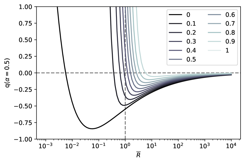
Figure 1: The $q-\overline{R}$ relation for $\alpha=0.5$. Colors indicate $f_{\bullet}$ and the values are shown in the legend. The overlap points between the $q-\overline{R}$ curves and the horizontal dashed line ($q=0$) indicates the $\overline{R}$ boundary of tidal disruption ($q>0$) and compression ($q<0$). The vertical line ($\overline{R}=1$) indicates the position of star cluster in the two-component potential. If $q\leq 0$ at $\overline{R}=1$, the cluster does not suffer tidal disruption.

For presentation convenience, we define

$$\overline{R}\equiv\frac{R}{R_{\mathrm{g}}},$$ (15)

where $\overline{R}$ represents the dimensionless distance to the galactic center normalized in the unit of $R_{\mathrm{g}}$. For a power-law galactic potential,

$$\frac{\Omega_{\mathrm{g}}^{2}}{\omega_{0}^{2}} =\begin{cases}\frac{3\overline{R}^{-\alpha}}{3-\alpha}&\text{for}~{}\alpha\neq 3\\ \frac{3\ln{\overline{R}}}{\overline{R}^{3}}&\text{for}~{}\alpha=3\end{cases}$$ (16)

$$\gamma_{\mathrm{g}}^{2} =\alpha\Omega_{\mathrm{g}}^{2}$$

where $\Omega_{\mathrm{g}}=\Omega(Rg)$, and $\gamma_{\mathrm{g}}=\gamma(R_{\mathrm{g}})$. For the point-mass (SMBH) potential at the same $R$,

$$\Omega_{\bullet}^{2} =\frac{GM_{\bullet}}{R^{3}}$$ (17)

$$\gamma_{\bullet}^{2} =3\Omega_{\bullet}^{2}$$

With the two components, the criterion of Equation 9 can be written as

$$\frac{f_{\bullet}(R_{\mathrm{g}})\gamma_{\bullet}^{2}+\left(1-f_{\bullet}(R_{\mathrm{g}})\right)\gamma_{\mathrm{g}}^{2}}{\left[f_{\bullet}(R_{\mathrm{g}})\Omega_{\bullet}^{2}+\left(1-f_{\bullet}(R_{\mathrm{g}})\right)\Omega_{\mathrm{g}}^{2}\right]^{3/4}}>\omega_{0}^{-1/2}.$$ (18)

After some algebra, this condition for tidal disruption (with $\alpha<\alpha_{\mathrm{max}}$) can be rewritten as

$$q =\frac{3\overline{R}^{3-\alpha}\alpha\left(f_{\bullet}(R_{\mathrm{g}})-1\right)^{2}+9^{2}}{\overline{R}^{3}\left(f_{\bullet}(R_{\mathrm{g}})-1\right)\left(\alpha-3\right)}$$ (19)

$$-\left(\frac{3\overline{R}^{3-\alpha}\left(f_{\bullet}(R_{\mathrm{g}})-1\right)^{2}+3f_{\bullet}(R_{\mathrm{g}})^{2}}{\overline{R}^{3}\left(f_{\bullet}(R_{\mathrm{g}})-1\right)\left(\alpha-3\right)}\right)^{\frac{3}{4}}>0.$$

The value of $R$ (or $\overline{R}$) at $q=0$ is equivalent to $R_{\mathrm{d}}$ in Equation (9) which again differs from the conventional tidal disruption radius of $R$ inferred from Equation (3) with $r_{\mathrm{t}}=r_{\rm cut}$. Hereafter, $R<R_{\mathrm{d}}$ refers to the sufficient criterion for tidal disruption.

We calculate $q-\overline{R}$ relation with $\alpha=0.5\ (<\alpha_{\mathrm{max}})$ for different $f_{\bullet}(R_{\mathrm{g}})$, as shown in Figure 1. The location of $R_{\mathrm{d}}$ indicates the outer boundary of the tidal disruption domain. When $f_{\bullet}(R_{\mathrm{g}})<0.3$, $R_{\mathrm{d}}<R_{\mathrm{g}}$, and thus, the cluster does not suffer tidal disruption. Figure 2 shows the relation of $R_{\mathrm{d}}$ and $f_{\bullet}(R_{\mathrm{g}})$ for three values of $\alpha$ (0.5, 0.9, and 2). For $\alpha=0.5$, the corresponding $f_{\bullet}(R_{\mathrm{g}})=1/3$ for $R_{\mathrm{d}}=R_{\mathrm{g}}$. With relative low SMBH-galaxy mass ratios, there is a range of galacto-centric distance from the SMBH smaller than that leads to cluster’s Roche-lobe overflow (the conventional necessary condition for tidal disruption), where the tidal perturbation on the cluster is compressive. For $\alpha=0.9$, which is close $\alpha_{\mathrm{max}}$ in the case of the single power-law potential, the minimum $R_{\mathrm{d}}\simeq R_{\mathrm{g}}$ and $f_{\bullet}(R_{\mathrm{g}})\approx 0.1$ when $R_{\mathrm{d}}=R_{\mathrm{g}}$. For $\alpha=2$, $R_{\mathrm{d}}>R_{\mathrm{g}}$ for all region of $f_{\bullet}(R_{\mathrm{g}})$ such that star clusters always suffer tidal disruption in this galactic+SMBH potential even in the limit of small SMBH-galaxy mass ratio. The sufficient criterion for tidal disruption would be satisfied when the necessary condition is met with $R_{\mathrm{d}}>R_{\mathrm{g}}$.

To validate this prediction, we perform 4 $N$-body simulations of W2 star clusters under the two-component (galaxy+SMBH) potential, where $\alpha=0.5$ and $f_{\bullet}(R_{\mathrm{g}})=0.01$, $0.1$, $1/3$, and $0.5$ respectively (§3.2). The corresponding $R_{\mathrm{d}}/R_{\mathrm{g}}\approx 0.0711,0.364,1.00$ and $1.56$ for these values of $f_{\bullet}(R_{\mathrm{g}})$, respectively. Similar to the discussion in §2.3.1, the small $R_{\mathrm{d}}$ value for small $f_{\bullet}(R_{\mathrm{g}})$ indicates the tidal compression can occur well inside the conventional galacto-centric tidal disruption distance. These clusters are again placed at $R_{\mathrm{g}}=100~{}r_{\mathrm{t}}$ with a circular orbit. We also perform another group of simulations with the same two-component potential, but placing the clusters on a circular orbit with different $R_{\mathrm{g}}$’s. This group of models represents a set of more general condition, where the values of $R_{\mathrm{g}}$ are independently specified, hence the ratio $r_{\mathrm{t}}/r_{\mathrm{cut}}$ differs from unity. Since $f_{\bullet}(R_{\mathrm{g}})$ increases when $R_{\mathrm{g}}$ decreases with the same potential, these models also have different $f_{\bullet}(R_{\mathrm{g}})$. The differences from the previous model set are that the clusters suffer a stronger tidal force and their orbital period is shorter when $R_{\mathrm{g}}$ is smaller. The cut-off radius $r_{\rm cut}$ of this set of cluster models need not be the tidal radius $r_{\mathrm{t}}$ (Eq. 3). In the limit $R_{\mathrm{g}}<100~{}r_{\mathrm{t}}$, a fraction of the cluster stars are initially placed inside $r_{\rm cut}$ but outside $r_{\mathrm{t}}$. With this general prescription, we investigate how the tidal effect determines the dynamical evolution of these stars. The initial value of $R_{\mathrm{g}}$ and corresponding $f_{\bullet}(R_{\mathrm{g}})$ are shown in Table 1. The results of the two model sets are shown in Section 3.2.

$R_{\mathrm{g}}[r_{\mathrm{t}}]$	5	10	20	40	60	80	100
$f_{\bullet}(R_{\mathrm{g}})$	0.948	0.762	0.361	0.091	0.035	0.017	0.010

Table 1: $R_{\mathrm{g}}$ and the corresponding $f_{\bullet}(R_{\mathrm{g}})$ for the star cluster models under a two-component potential ($\alpha=0.05$).

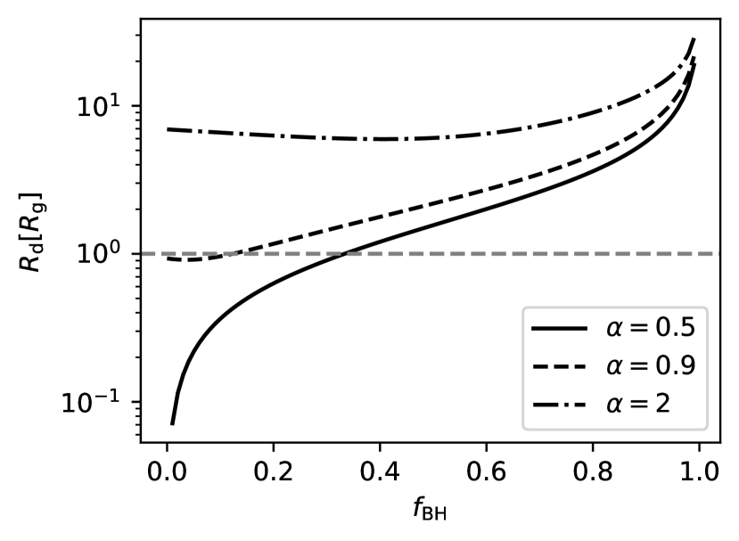
Figure 2: The $f_{\rm BH}(\equiv f_{\bullet})-R_{\mathrm{d}}$ relation of the two-component potential. Three values of $\alpha$ are shown. When $f_{\rm BH}$ is larger than the overlap point between the dashed line ($R_{\mathrm{d}}=R_{\mathrm{g}}$) and the curves, the cluster suffer tidal disruption. For $\alpha=2$, the cluster always suffers tidal disruption.

2.3.3 Time-dependent background potential for clusters with slowly decaying orbit

Star clusters undergo orbital decay due to dynamical friction and endure increasingly strong external potential. In order to represent this effect, we smoothly increase the scaled mass which contributes to the galactic potential in the co-moving frame centered on the cluster. Note that this generic scaling prescription is equivalent to the evolving external tidal field imposed on an in-spiraling stellar cluster in a static galactic potential. It does not correspond an actual (physical) mass gain for the galaxy and the SMBH. For a reference, we also integrate the orbit of a point-mass satellite in the single component potential with the Chandrasekhar’s dynamical friction, the results are presented and discussed in Appendix. For the time-dependent two-component potential, the masses of the SMBH and the galactic bulge should increase with the same rate to correctly represent the static potential. But this scaling prescription does not mean that $f_{\bullet}(R)$ is a constant of radius. As star clusters approach to the center, $R$ decreases while $f_{\bullet}(R)$ increases.

We consider an evolved power-law potential (with $\alpha=0.5$) and an evolved two-component potential (with $\alpha=0.5$ and $f_{\bullet}(R_{\mathrm{g}})=0.01$) where $\rho_{\mathrm{g0}}$ increases exponentially as

$$\rho_{\mathrm{g0}}(t)=\rho_{\mathrm{g0}}(0)e^{\mathcal{R_{\mathrm{\rho}}}t}.$$ (20)

By changing $\mathcal{R_{\mathrm{\rho}}}$, we can investigate clusters with different in-spiraling time scales (§4.1). When $\mathcal{R_{\mathrm{\rho}}}$ is small, $T_{\mathrm{rh}}$ is less than the in-spiral time and star cluster follows a tightly wrapped spiral pathway. We investigate three values of $\mathcal{R_{\mathrm{\rho}}}$: 0.033, 0.065 and 0.13 $T_{\mathrm{rh0}}^{-1}$, for both power-law and two-component potentials. Meanwhile, when massive GC’s (with the same internal density) sink into the galactic center via dynamical friction, their inspiral time scale can be much shorter than its $T_{\mathrm{rh}}$. Thus, we include three additional models with the power-law potential and $\mathcal{R_{\mathrm{\rho}}}$ of 4.2, 8.3, 17 $T_{\mathrm{rh0}}^{-1}$. The results of simulations are shown in § 4.1 (Fig. 11).

Our $N$-body models assume initial number of stars, $N=1000$. To validate that the tidal compression feature is independent of $N$, we also include a group of simulations with $N=10000$ and the same total mass (Fig. 10). The clusters move in power-law potentials with $\alpha=0.5$ and $\mathcal{R_{\mathrm{\rho}}}=0,0.17$ and $21T_{\mathrm{rh0}}^{-1}$, where $0$ represents a static potential. The initial position is the same where $R_{\mathrm{g}}=100r_{\mathrm{t0}}$.

2.3.4 Time-dependent background potential for clusters with highly eccentric orbits

We investigate two sets of clusters moving on elliptical orbits around some static (both power-law and two-component) tidal potentials. We adopt a modest eccentricity in the first set by setting the initial tangential velocity of the cluster to be half of that in a circular orbit. We consider a nearly parabolic set by setting a small initial tangential velocity (about 8 percent of the circular one). Table 2 summarizes the model parameter of all simulations in this study. The results of these simulations are shown in § 4.3.

Profile	Potential	Varying parameters	Number of models
Homo.	power-law	$\alpha=0.5,1,2$, point-mass, NoTide	5
King	power-law	$\alpha=0.5,1,2$, point-mass, NoTide	15
		$W_{0}=2,6,8$ for each galactic potential
King	power-law	$\alpha=0.5,1,2$, point-mass, NoTide	30
$W_{0}=2$		6 groups of different random seeds
	two-component	$f_{\bullet}(R_{\mathrm{g}})=0.01,0.1,1/3,0.5$	4
	$\alpha=0.5+f_{\bullet}=0.01$	$R_{\mathrm{g}}[r_{\mathrm{t}}]=5,10,20,40,60,80,100$	7
	secular decay, $N=1000$	$\mathcal{R_{\mathrm{\rho}}}=0.033,0.065,0.13[T_{\mathrm{rh0}}]$	6
		$\alpha=0.5$, $\alpha=0.5+f_{\bullet}=0.01$
		$\mathcal{R_{\mathrm{\rho}}}=4.2,8.3,17~{}[T_{\mathrm{rh0}}]$	3
	secular decay, $N=10000$	$\mathcal{R_{\mathrm{\rho}}}=0.033,0.065,0.13~{}[T_{\mathrm{rh0}}]$ for $\alpha=0.5$, NoTide	4
	eccentric orbit	eccentric, nearly-radial	4
		$\alpha=0.5$, $\alpha=0.5+f_{\bullet}=0.01$

Table 2: Initial conditions of all simulations. ”Homo.” and ”King” represent the homogeneous and Michie (1963)-King (1966) profiles, respectively. $\alpha=0.5$ and $\alpha=0.5+f_{\bullet}=0.01$ represent the power-law potential with $\alpha=0.5$ and the two-component potential with $\alpha=0.5$ and $f_{\bullet}(R_{\mathrm{g}})=0.01$, respectively.

3 Clusters on nearly circular orbit around the galaxy

3.1 Static one-component galactic potential

3.1.1 Homogeneous sphere

Figure 3 shows the morphology of star clusters with the homogeneous sphere (§2.2.2) in a power-law potential (§2.3.1) at $4~{}T_{\mathrm{rh0}}$ and the evolution of different Lagrangian radii ($r_{\mathrm{lagr}}$) and the core radius ($r_{\mathrm{c}}$). We separate the tidal response from the clusters’ internal two-body-relaxation effects using comparisons between clusters embedded in the external tidal field and the appropriate NoTide calibration model. For these isolated star clusters (last panel), the system’s core contracts within $0.1~{}T_{\mathrm{rh0}}$ or $2~{}T_{\mathrm{cr0}}$ ($T_{\mathrm{rh0}}\approx 18.3~{}T_{\mathrm{cr0}}$, where $T_{\mathrm{cr0}}$ is the initial crossing time in Eq. 1), then expands and virializes to its original structure after about $4~{}T_{\mathrm{cr0}}$. During the subsequent quasi-stable relaxation, the inner radii ($<r_{\mathrm{h}}\equiv r_{\mathrm{lagr}}(50\%)$, the half-mass radius) contract while the outer radii ($>r_{\mathrm{h}}$) expand. This evolution is a direct consequence of two-body relaxation(Spitzer, 1987; Heggie & Hut, 2003) and we use this model for calibrator to accentuate the tidal influence. The effects of tidal compression and disruption respectively leads to the deceleration and acceleration in the expansion of the outer $r_{\mathrm{lagr}}>r_{\rm h}$.

In the proximity of a point-mass potential, clusters with $r_{\rm cut}\gtrsim r_{\mathrm{t}}$ quickly suffers total tidal disruption within one $T_{\mathrm{rh0}}$. For single power-law potentials with various values of $\alpha$ (Eq. 6), the clusters become less vulnerable to tidal disruption in the limit of small $\alpha$. In the case of $\alpha=1$, which is close to $\alpha_{\mathrm{max}}$, the radii $r_{\mathrm{lagr}}$ within the half mass radius $r_{\mathrm{h}}$ follow similar evolutionary paths as those in the NoTide calibration model without the galactic potential. Nevertheless, the outer radii for this model show modest amount of tidal removal. In contrast, the model with $\alpha=0.5$ shows the characteristics of tidal compression, where outer radii do not expand. For the $\alpha=2$ model and the point-mass potential, both the sufficient and necessary conditions for tidal disruption are satisfied and the cluster’s $r_{\mathrm{lagr}}$ expands faster than their equivalent radii for the NoTide calibration model. This $\alpha$-dependence is consistent with the analytic calculation carried out by Ivanov & Lin (2020).

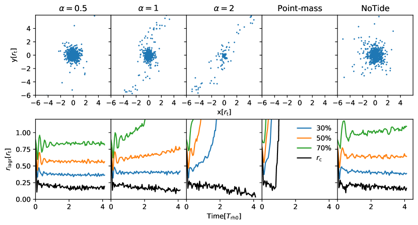
Figure 3: The morphology at about $4~{}T_{\mathrm{rh0}}$ (upper panel) and the evolution of Lagrangian radii ($r_{\mathrm{lagr}}$) and core radii ($r_{\mathrm{c}}$) of star clusters with the spherical symmetric homogeneous mass-density distribution (lower panel). The columns show different galactic potentials. The first three represent power-law spherically symmetric potentials with different $\alpha$ (see Equation 6). The last two show the point-mass potential and the reference without tidal field (NoTide). Colors in the lower panels indicates the mass fractions of $r_{\mathrm{lagr}}$, except that the red color represents the core radius $r_{\mathrm{h}}$.

3.1.2 Clusters with a Michie-King initial density distribution

Figure 4: The evolution of Lagrangian radii of star clusters with different $W_{0}$ of King model. The galactic potential set is the same as that in Figure 3.

Figure 4 show the evolution of $r_{\mathrm{lagr}}$ and $r_{\mathrm{c}}$ for models with Michie-King profiles (§2.2.3) in the clusters and power-law potentials (§2.3.1) for the host galaxy. All models are evolved for more than $80~{}T_{\mathrm{rh0}}$. In the absence of galactic potential, the NoTide calibration model shows core collapse after the first $20~{}T_{\mathrm{rh}}$. During the long-term evolution in the post-core-collapse phase, all $r_{\mathrm{lagr}}$ expands because binary systems form in the core and stars are ejected from the core through binary-single-star close encounters.

For the $\alpha=2$ as well as the point-mass galactic potential, the clusters with small $W_{0}$ are rapidly disrupted. Similar to the case in Figure 3, the evolution for $\alpha=1$ power-law potential is close to that without galactic potential. Although the half-mass radius $r_{\rm h}(\equiv r_{\mathrm{lagr}}(50\%))$ in the W2, W6, and W8 clusters with $\alpha=0.5$ galactic potential increases with time, its expansion rate is slower than that in the NoTide calibration model. This evolutionary pattern is the characteristics of tidal compression. Comparison between Figures 3 and 4 indicate that the internal density profile of star clusters does not significantly affect the criterion for tidal disruption and compression (Equation 9). Since the structure evolution of the W2 model is most sensitive to the galactic potential, we apply this density profile as a default model for the star clusters in the following analysis with different galactic potentials.

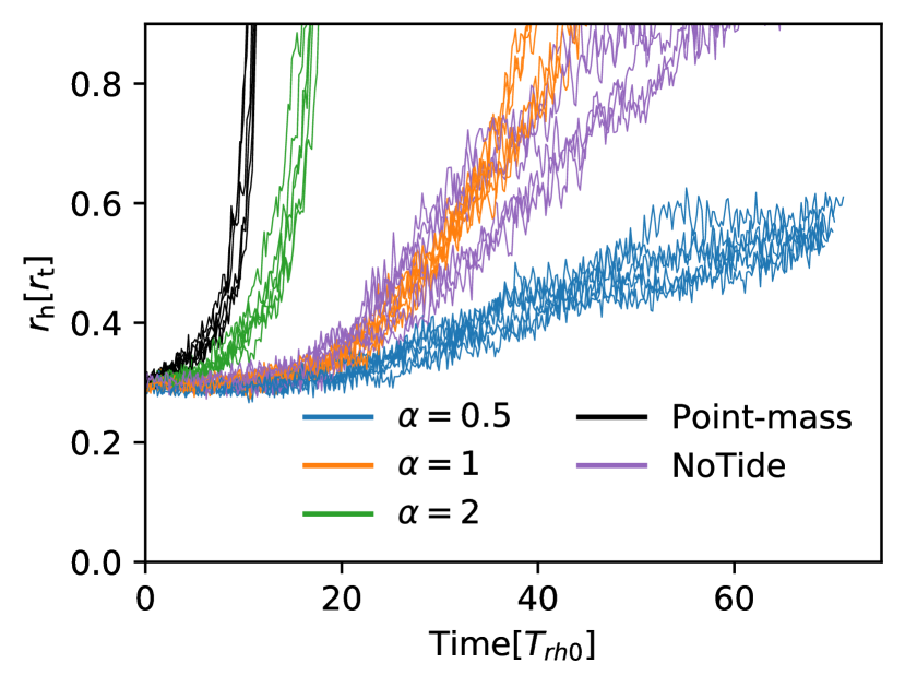
Figure 5: The evolution of $r_{\mathrm{h}}$ of star clusters with $W_{0}=2$, different galactic potentials and 6 different sets of random seeds for initial conditions. Each curve represents one simulation. Curves with the same color have the same potential.

Models with the same density profile (i.e. identical initial stellar positions and velocities) in Figure 3 and 4 are embedded in different galactic potentials. Keeping the same initial condition can reduce the stochastic scatter due to the low number of stars. To confirm that the tidal compression is robust, we perform a set of tested models with 6 different random seeds, and compare how $r_{\mathrm{h}}$ evolves under different galactic potential. The results in Figure 5 show that the stochastic scatter due to the random seeds is much smaller than the difference caused by tidal effect imposed by various prescriptions for the galactic potentials.

3.2 A two-component model for the galaxy-SMBH composite potential

Figure 6 shows the evolution of $r_{\mathrm{lagr}}$ and $r_{\mathrm{c}}$ for the two-component models of $\alpha=0.5$ with four values of $f_{\bullet}$ (§2.3.2). Based on their comparison with the NoTide calibration model, the clusters surrounded by the $f_{\bullet}=0.01$ and $0.1$ potential are tidally compressed. For relative high SMBH-galaxy mass ratios (with $f_{\bullet}=1/3$ and $0.5$ at $R_{\mathrm{d}}=R_{\mathrm{g}}$), the sufficient criterion for tidal disruption is satisfied when the conventional, Roche-lobe-filling, necessary condition is met and the cluster’s $r_{\mathrm{lagr}}$ expand faster than their equivalent radii for the NoTide calibration model. These results are consistent with the value of $f_{\bullet}$ for the $R_{\mathrm{d}}=R_{\mathrm{g}}$ transition inferred from Figure 2 and Equation (19). The evolution of $r_{\mathrm{lagr}}$ for both homogeneous and Michie-King profiles show that the outermost $r_{\mathrm{lagr}}$ is most sensitive to the tidal effect. To simplify the comparison, for the following analysis of tidal effect, we only show the evolution of $r_{\mathrm{lagr}}$ with the mass fraction of 90 percent.

When $R_{\mathrm{g}}=100~{}r_{\mathrm{cut}}$, a special condition occurs in which star cluster’s $r_{\mathrm{t}}$ overlaps $r_{\mathrm{cut}}$ of the King profile. We consider more general cases with this special condition as a reference point. In models with $R_{\mathrm{g}}<100~{}r_{\mathrm{cut}}$, a fraction of the cluster stars are initially located outside $r_{\mathrm{t}}$ (Table 1). As $R_{\mathrm{g}}$ changes, the corresponding $f_{\bullet}$ also varies. In the range $R_{\mathrm{g}}\geq 40~{}r_{\mathrm{t}}$ ($f_{\bullet}<1/3$), $r_{\mathrm{lagr}}(90\%)$ increases slower than that of the NoTide calibration model (Fig. 7). This difference suggests a tidal compression process which is also consistent with critical value of $f_{\bullet}$ for the $R_{\mathrm{d}}=R_{\mathrm{g}}$ transition (Fig. 2). After about $8~{}T_{\mathrm{rh0}}$, $R_{\mathrm{g}}\leq R_{\mathrm{d}}\simeq 40~{}r_{\mathrm{t}}$, $r_{\mathrm{lagr}}(90\%)$ of increases faster than that of the NoTide calibration model, which suggests a tidal disruption feature. Similar values of $R_{\mathrm{d}}$ are obtained for models with larger initial $R_{\mathrm{g}}$, albeit the transition take place at later times. These results suggest that stars outside $r_{\mathrm{t}}$ suffer both tidal compression and disruption effects at different stages.

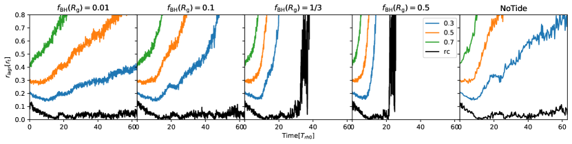
Figure 6: The evolution of Lagrangian radii of star clusters in the two-component potential with $\alpha=0.5$. Columns show different mass ratios between SMBH and galactic background. The model without galactic potential is shown in the last column.

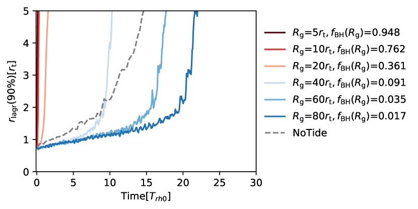
Figure 7: The evolution of $r_{\mathrm{lagr}}(90\%)$ for star clusters in the two-component potential with different $R_{\mathrm{g}}$ (see Table 1). The NoTide model is shown as dashed curve for a reference.

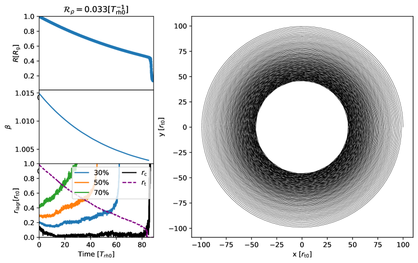
Figure 8: In the left panel from the top to the bottom: the distance ($R$) to the galactic center, $\beta$ from Equation 22 with the $P$ calculated at $r_{\mathrm{t}}$, and the evolution of $r_{\mathrm{lagr}}$ and $r_{\mathrm{c}}$. The star cluster evolve in an time-dependent power-law potential with $\alpha=0.5$ and $\mathcal{R_{\mathrm{\rho}}}\approx 0.033~{}T_{\mathrm{rh0}}^{-1}$. In the right panel: the trajectory of the star cluster in the orbital plane of the galactic frame. The length unit $r_{\mathrm{t0}}$ is the initial $r_{\mathrm{t}}$. After the complete tidal disruption where $r_{\mathrm{c}}\gg r_{\mathrm{t}}$, no physical core exists, and a transition in the orbital trajectory appears near $R=0.4~{}R_{\mathrm{g}}$.

4 Time-dependent potential due to orbital decay

In this section, we investigate clusters’ evolution in some time-dependent potentials including those due to their inward migration or due to their eccentric orbits. For the former case, we artificially increase the scaled masses of the galaxy and the SMBH as a generic approximation to the effect of orbital decay due to dynamical friction (§2.3.3). The physical mass and potential distribution of the host galaxy that the model represents do not actually change over time. To characterize the star clusters’ initial structure, we choose the W2 density profile since its response to the galactic tidal effect is more pronounced.

4.1 Clusters with monotonic secular orbital decay

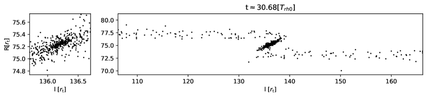
Figure 9: The projected morphology of the star cluster shown in Figure 8 at about $30.68~{}T_{\mathrm{rh0}}$. The polar coordinate in the galactic orbital plane ($x$-$y$) is used, where $l=R\phi$ and $\phi$ is angle. The left panel is the zoomed-in image.

We investigate how $\mathcal{R_{\mathrm{\rho}}}$ affects the evolution of star clusters under the time-dependent potential described by Equations 20 and 22. To guide our interpretation, we first analyze how the local density of the galactic background varies as a function of $\mathcal{R_{\mathrm{\rho}}}$. We define $\Delta\rho_{\mathrm{g}}$ to be the maximum variation in the circumscribed galactic mass density as a typical star revolves around a cluster. For a static power-law galactic potential, it can be approximated as:

$$\Delta\rho_{\mathrm{g}} \simeq\rho_{\mathrm{g0}}\left[\left(\frac{R_{\mathrm{g}}}{R-\Delta R}\right)^{\alpha}-\left(\frac{R_{\mathrm{g}}}{R+\Delta R}\right)^{\alpha}\right]$$ (21)

$$\approx 2\alpha\rho_{\mathrm{g0}}R_{g}^{\alpha}\Delta R\frac{1}{R^{\alpha+1}}$$

where $\Delta R$ is the maximum difference of $R$ for the star (traveling from the minimum of to the maximum of $R$), and the approximation of $\Delta\rho_{\mathrm{g}}$ is derived by taking the first-order Taylor expansion of Equation 6. If $R$ does not change, i.e. $\Delta R$ changes sign throughout each orbit, the net amount of $\Delta\rho_{\mathrm{g}}$ would vanish.

For a time-dependent potential resulting from the cluster’s orbital decay, clusters travel from $R-\Delta R$ to $R+\Delta R$ with a finite $\Delta R\propto R^{-\beta}$ where $\beta=e^{\mathcal{R_{\mathrm{\rho}}}P/2}$ during each orbital period $P$. The corresponding finite net residual

$$\Delta\rho_{\mathrm{g}} =\rho_{\mathrm{g0}}\left[\left(\frac{R_{\mathrm{g}}}{R-\Delta R}\right)^{\alpha}-e^{\frac{\mathcal{R_{\mathrm{\rho}}}P}{2}}\left(\frac{R_{\mathrm{g}}}{R+\Delta R}\right)^{\alpha}\right]$$ (22)

$$\approx\rho_{\mathrm{g0}}R_{g}^{\alpha}\left[\frac{1-\beta}{R^{\alpha}}+\left(1+\beta\right)\frac{\alpha\Delta R}{R^{\alpha+1}}\right].$$

In the limit $\mathcal{R_{\mathrm{\rho}}}=0$ and $\beta=1$, Equation(22) reduces to Equation(21) with no net residual $\Delta\rho_{\mathrm{g}}$. Provided $\beta$ is slightly larger than unity, stars in the clusters adjust to adiabatic modifications in the strength of the host galaxy’s tidal potential.

4.2 Tidal disruption along the course of orbital decay

Figure 8 shows the evolution of $R$, $\beta$, $r_{\mathrm{lagr}}$, $r_{\mathrm{c}}$ and $r_{\mathrm{t}}$ for the model with a power-law potential in which $\alpha=0.5$, $f_{\bullet}(R_{\mathrm{g}})=0.01$, and $\mathcal{R_{\mathrm{\rho}}}\approx 0.033~{}T_{\mathrm{rh0}}^{-1}$. As the scaled mass of the galaxy increases, the star cluster spirals towards the galactic center. Note that the cluster’s orbital trajectory obtained with idealized, generic prescription qualitatively agrees with the numerical integration of the conventional dynamical friction formulae (Fig. 18). As $R$ decreases, the cluster’s corresponding $r_{\mathrm{t}}$ shrinks. After the cluster’s core collapse, the outer $r_{\mathrm{lagr}}(\geq r_{\rm h})$ continues to expand. During the entire course of evolution, $\beta$ is close to unity and decreases monotonically (Eq. 22). The system initially evolves in an adiabatic manner. As different $r_{\mathrm{lagr}}$’s increase beyond $r_{\mathrm{t}}$, their expansion rate accelerates. This pattern is an indication that stars outside $r_{\mathrm{lagr}}$ have suffered tidal disruption, analogous to that of models with $R_{\mathrm{d}}=40~{}r_{\mathrm{t}}$ in Figure 7. Eventually, when $r_{\mathrm{c}}>r_{\mathrm{t}}$, the cluster completely and the determination of the cluster center becomes invalid. After core disruption, dynamical friction ceases to be effective (Fellhauer & Lin, 2007) and the evolution of $R$ can no longer represents the position of the star cluster.

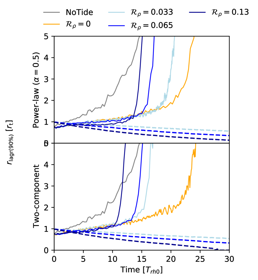
Figure 10: The evolution of $r_{\mathrm{lagr}}(90\%)$ (solid lines) and $r_{\mathrm{t}}$ (dashed lines) for models with time-dependent power-law potential (upper panel) and two-component potential (lower panel). The reference models with static potentials and NoTide calibration model are shown as grey and orange colors, respectively. The value of $\mathcal{R_{\mathrm{\rho}}}$ are in the unit if $T_{\mathrm{rh0}}^{-1}$.

To understand how tidal disruption occurs in the limit $r_{\mathrm{lagr}}>r_{\mathrm{t}}$, we plot, in Figure 9, the morphology of the cluster at about $30.68~{}T_{\mathrm{rh0}}$ when the half-mass radius almost reaches $r_{\mathrm{t}}$. Although the cluster is tidally compressed in the $R$ direction, it is also distorted along the tangential direction with some phase lag and two tidal tails form. Thus, both radial compression and azimuthal disruption determine the evolution of star clusters. This illustration also explains why the evolution of $r_{\mathrm{lagr}}$ depends on the clusters’ orbits as shown in Figure 7.

With a follow-up study, we compare models with different $\mathcal{R_{\mathrm{\rho}}}$ and show the evolution of $r_{\mathrm{lagr}}(90\%)$ and $r_{\mathrm{t}}$ in Figure 10. Here the three $\mathcal{R_{\mathrm{\rho}}}$ values are small such that the cluster’s in-spiral time is much longer than $T_{\mathrm{rh}}$ and the cluster’s orbits undergo tightly wrapped decay. Both the time-dependent power-law potentials and the two-component potentials are investigated. For the two-component (galaxy+SMBH) potentials, both the scaled mass of the galaxy and the SMBH increase with the same $\mathcal{R_{\mathrm{\rho}}}$ , i.e, $f_{\bullet}(R_{\mathrm{g}})$ does not change with time. In this case, as $R$ (or equivalently $\overline{R}={R}/{R_{\mathrm{g}}}$) of the star cluster decreases, $f_{\bullet}(R)$ increases. The corresponding $R$ for $f_{\bullet}(R)=1/3$ is about $0.21~{}R_{\mathrm{g}}$.

With a larger $\mathcal{R_{\mathrm{\rho}}}(=0.13)$, $r_{\mathrm{lagr}}(90\%)$ shows more pronounced characteristics of tidal compression compared with the case of the NoTide calibration and the static ($\mathcal{R_{\mathrm{\rho}}}=0$) power-law potential. But the system also reaches the disruption phase earlier as $r_{\mathrm{t}}$ shrinks faster than the model with smaller $\mathcal{R_{\mathrm{\rho}}}$. In general, clusters dissolute slightly faster under the two-component (galaxy+SMBH) than the power-law galactic potential.

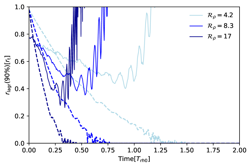
Figure 11: The solid and dashed lines represent the same quantities as in Figure 10. Only models with power-law potential and large $\mathcal{R_{\mathrm{\rho}}}$ are presented here.

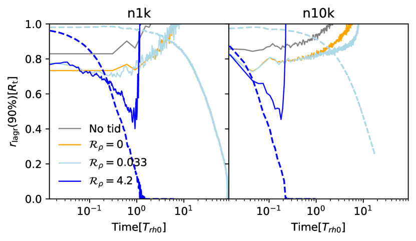
Figure 12: Comparing the models with different $N$. The plotting style is similar to Figure 10.

Figure 11 shows another set of three models with much larger $\mathcal{R_{\mathrm{\rho}}}$, where $T_{\mathrm{rh}}$ is longer than the in-spiral time. In these cases, $r_{\mathrm{lagr}}(90\%)$ contracts slightly before any significant expansion. This evolutionary pattern clearly indicates the onset of tidal compression before disruption. Moreover, $r_{\mathrm{lagr}}(90\%)$ continues to decrease for a while after $r_{\mathrm{t}}$ has become smaller than it. This tendency suggests that tidal compression in the radial direction can cause some delays in the tidal disruption of the cluster in the azimuthal direction and clusters in galaxies with sufficiently small $\alpha$ can preserve their integrity after their orbits have decayed, with modest $f_{\bullet}(R)$, inside the conventional Roche-lobe-filling tidal disruption radius. Nevertheless, they eventually disintegrate due to the tidal dispersal in the azimuthal direction.

Figure 12 compares the models with different $N$. With 10 times larger $N$, the evolution of $r_{\mathrm{lagr}}$ has nearly identical tendency (including the NoTide calibration model), albeit the evolution timescale is slight shorter for the $\mathcal{R_{\mathrm{\rho}}}=4.2$ case.

4.3 Nearly-radial orbits

To explore the possibility of injecting the debris stars from the disrupted clusters to the immediate neighborhood of SMBHs, we compare models with modestly and highly eccentric orbits as described in §2.3.4. Figure 13 show the spatial distribution of stars at about $92~{}T_{\mathrm{rh0}}$ for four models with a static ($\mathcal{R_{\mathrm{\rho}}}=0$), power-law ($\alpha=0.5$) and a static, two-component potential ($\alpha=0.5$ and $f_{\bullet}(R_{\mathrm{g}})=0.01$).

For the modestly eccentric orbit, long tidal tails appear between $R\simeq 50-100~{}r_{\mathrm{t0}}$ but no cluster stars enter into the region with $R\lesssim R_{\mathrm{d}}\simeq 40~{}r_{\mathrm{t0}}$ in both power-law and two-component (with SMBH) galactic potentials. For the cluster with a highly-eccentric (nearly-plunging) orbit, the outcome of peri-galacticon passage is very different for these two types of galactic potentials. Under the power-law potential the cluster stars are distributed along narrow bridges and tails along the original orbit of the star cluster. Under the two-component (galaxy+SMBH) potential, the disrupted stars widely spread out in all regions. This feature indicates that the SMBH has a strong scattering impact on the stars in the tidal debris of the disrupted star clusters as they venture to its proximity.

Figure 14 shows the evolution of $r_{\mathrm{lagr}}(90\%)$ and $r_{\mathrm{t}}$, analogous to Figure 10. For both modestly-eccentric and nearly-radial models under the power-law potential, the effect of tidal compression before $r_{\mathrm{lagr}}(90\%)<r_{\mathrm{t}}$ remains apparent. The nearly-radial model has a rapid $r_{\mathrm{h}}$ expansion due to a strong mass loss which also lead to a fast reduction of $r_{\mathrm{t}}$. Under the tidal influence of the SMBH, the cluster with a nearly-radial orbit quickly suffers severe tidal disruption.

The ratio between the period of star clusters on a circular orbit at $R_{\mathrm{d}}=100~{}r_{\mathrm{t}}$ and $T_{\mathrm{rh0}}$ is about 1.57. The modestly-eccentric clusters have shorter orbital periods. The frequent oscillation of $r_{\mathrm{lagr}}$ and $r_{\mathrm{t}}$ is due to the cluster’s motion between apo- and peri-galactic passages. For both the modestly-eccentric and nearly-radial orbits, the tidal disruption occur smoothly over a few orbits.

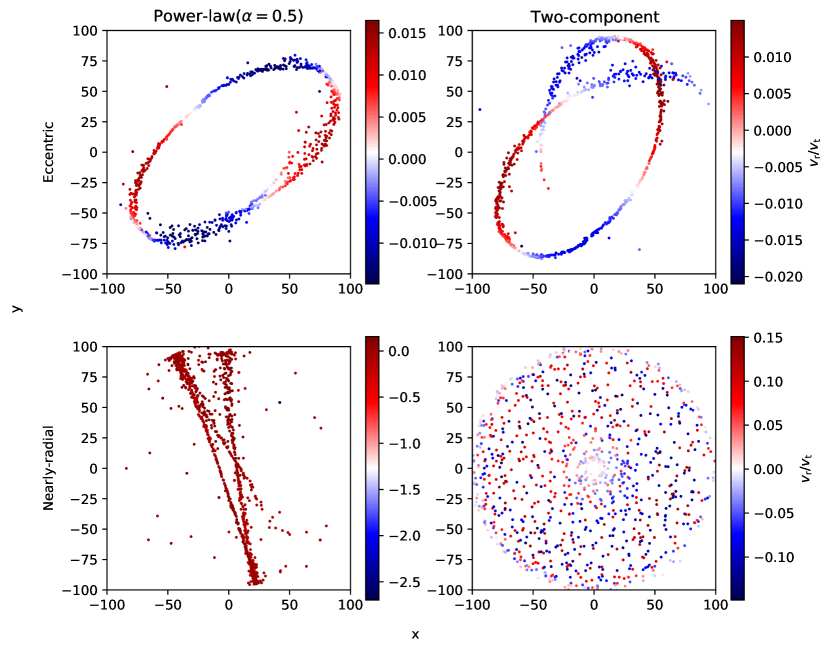
Figure 13: The positions of stars in the orbital plane ($x$-$y$) in the galactic frame. Colors represent the ratio between radial and tangential velocities of stars. The upper and lower panels show models with eccentric and nearly-radial orbits, respectively. The left and right columns show the power-law and two-component potentials, respectively.

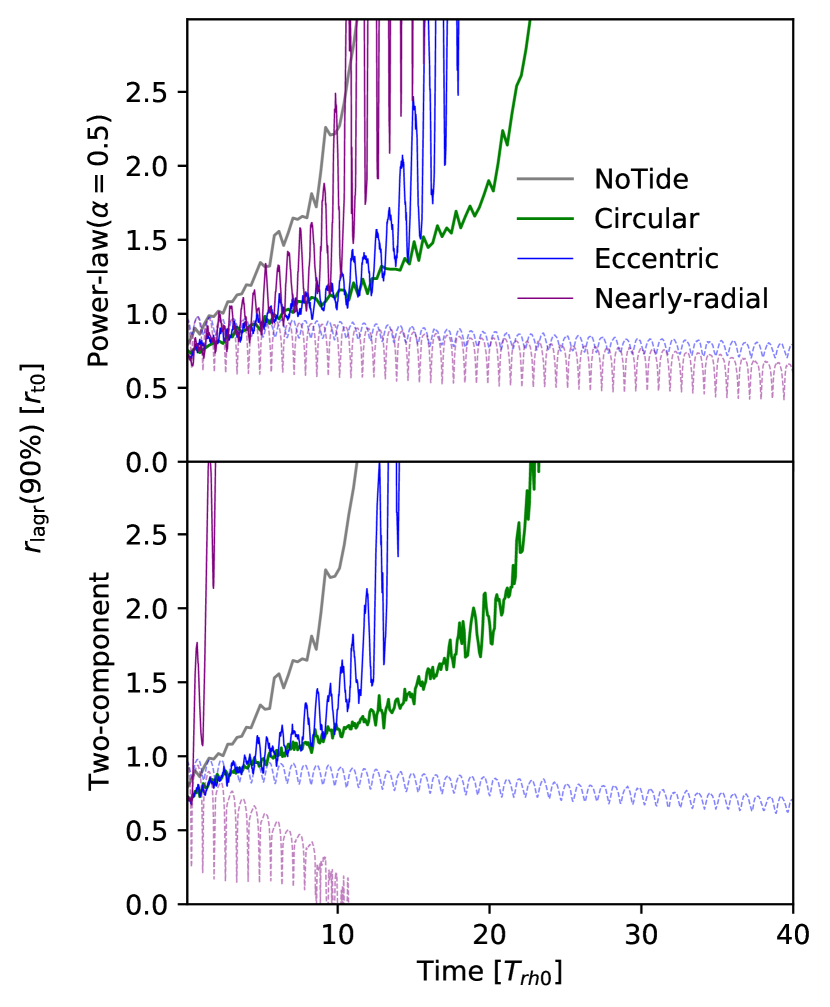
Figure 14: The evolution of $r_{\mathrm{lagr}}(90\%)$ (solid lines) and $r_{\mathrm{t}}$ (dashed lines) for models with different orbits in a power-law ($\alpha=0.5$) and a static two-component potentials are compared. The reference model with no tidal field is shown as grey color. The models with a circular, an eccentric and a nearly-radial orbits are shown with different colors.

Figure 15 shows the radial distribution of stars relative to the galactic center at $92~{}T_{\mathrm{rh0}}$. The peak of the distribution indicates the location of star cluster. There are no stars within $R\simeq 40~{}r_{\mathrm{t0}}$ for the models with modestly-eccentric orbit. But, the SMBH has a strong impact on the distribution of stars for the cluster with nearly-radial orbit. A significant fraction of stars can reach inside the tidal disruption distance ($R_{\mathrm{d}}\simeq 40~{}r_{\mathrm{t0}}$). In contrast, in the case with gradually in-spiraling decay, dynamical friction is quenched when a star cluster is completely tidally disrupted near $R_{\mathrm{d}}$ so that only a few stars can reach inside $R_{\mathrm{d}}$ (Fig. 8).

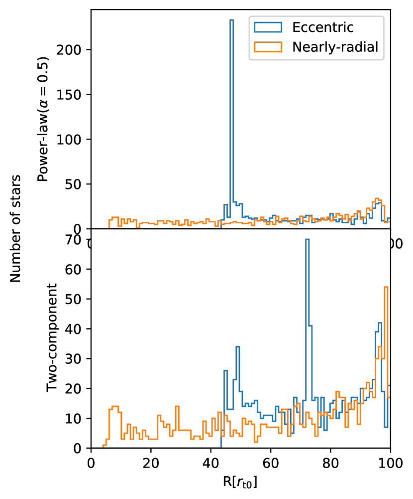
Figure 15: The radial distribution of stars referring to the galactic center for models with eccentric and radial orbits. The upper and lower panel show models with a power-law ($\alpha=0.5$) and a static two-component potentials respectively.

Figure 16 shows the $x$-$y$ and distribution of stars for models with eccentric and radial orbits and different potentials at $92~{}T_{\mathrm{rh0}}$. For the single power-law potential, clusters still keep a narrow shape when $\alpha=0.5$ but their tidal debris spreads over much more extended region in the model with $\alpha=2$. This difference provides another evidence that tidal compression in galaxies with low $\alpha$ density distribution delays the disruption of clusters.

Due to fast differential precession, the stars removed from the cluster quickly disperse to establish a nearly isotropic (in the cluster’s original orbital plane) distribution. Nevertheless, they retain the kinematic properties of their original host clusters. Figure 17 shows the $v_{\mathrm{R}}$-$R$ distribution for the same group of models. All models show a clearly correlated patterns. Models with $\alpha=2$ show large $v_{\mathrm{R}}$. In comparison, more stars occupy the central region of the galaxy in models with $\alpha=0.5$ (Fig. 16) where they are near their orbital peri-center with smaller $v_{\mathrm{R}}$ (Fig. 17). In principle, this distribution can be extracted from the observed radial velocity proper motion of stars near the galactic center and be used to identify lost members of tidally disrupted clusters.

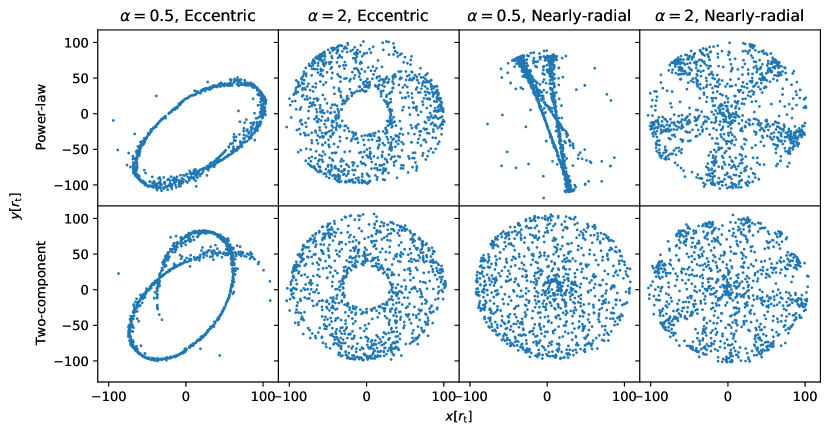
Figure 16: The $x$-$y$ distribution of stars referring to the cluster center at $92~{}T_{\mathrm{rh0}}$ for models with eccentric and radial orbits. The upper and lower panel show models with a power-law and a static two-component potentials respectively. For the power-law component, results of $\alpha=0.5$ and $2$ are compared for both eccentric and radial orbits.

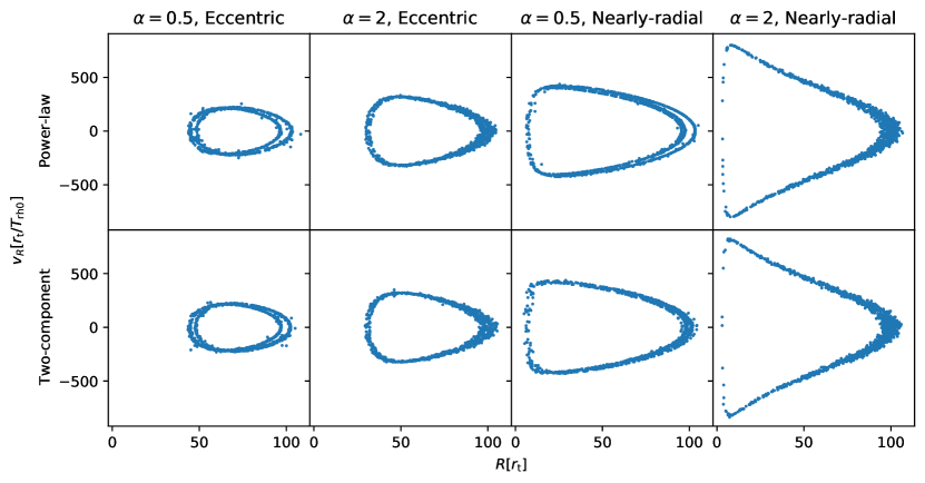
Figure 17: Similar to Figure 16, but the radial velocity vs. $R$ of stars are shown.

5 Summary and Discussions

This work is primarily motivated by the possibility of populating the innermost region of galaxies by inward migration of stellar clusters formed elsewhere. The main physical processes which may lead to such migration includes dynamical friction, mergers, and secular perturbation by galactic companions and satellites (see references of previous investigations in §1). The main focus of this paper is whether clusters can reach the central region. To highlight this outstanding issue, we apply our simulated results to the interpretation of observational data. Do et al. (2020) found two populations of stars near (within $\sim 4$ pc in projected distance from) the Galactic center, separated by different velocity dispersion and metallicity. We revisit the suggestion that these diverse stellar populations are the debris of disrupted stellar cluster. The mass contained in the NSC in this region is $M(R)\sim$ a few $10^{7}M_{\odot}$ in addition to that of the Sgr^⋆ SMBH. If the parent clusters have $M_{\mathrm{sc}}\sim 1-2\times 10^{6}M_{\odot}$, $r_{\mathrm{h}}\sim$ a few pc, and $r_{\rm cut}\sim{\mathcal{O}}(10r_{\mathrm{h}}$) (those of the most massive globular cluster in the Galaxy), their conventional galacto-centric tidal disruption distance would be at least an order of magnitude larger than the location where diverse stellar populations were found (§2.2.2 and §2.2.3). Even with the most-compact (and relative low-mass) cores of known globular clusters, their conventional tidal radius $r_{\mathrm{t}}$ at $R\sim$ a few pc is $\lesssim$ their $r_{\mathrm{c}}$ (Eqs. 3 and 4), i.e. they are expected to have disrupted at larger galacto-centric distances. Note that the existence of a hypothetical IMBH at the center of an in-spiral star cluster (Arca-Sedda & Gualandris, 2018) can provide a lower limit of $r_{\mathrm{t}}$ depending on its mass ($M_{\mathrm{IMBH}}$). For $M_{\mathrm{IMBH}}\simeq 10^{4}M_{\odot}$, the corresponding $r_{\mathrm{t}}\approx 0.3$ pc at $R=4$ pc from the Galactic center, which is roughly the core radius of a dense star cluster. Thus, an IMBH may help to prevent the core from tidal disruption and bring it further towards the center of the Galaxy, albeit relatively small number of cluster stars may migrate to the last few pc from Sgr A^⋆.

Our first attempt to bypass this migration barrier (imposed by the conventional, Roche-lobe-filling, necessary tidal disruption condition) is to consider the possibility of tidal compression. In this work, we carry out a series $N$-body simulations of equal-mass star clusters under different types of galactic potential, in order to determine the sufficient criterion for compressive tidal perturbation in addition to the conventional necessary Roche-lobe-filling condition for tidal disruption of satellite stellar systems. We find that for a smooth power-law, galaxy-only, potential where $\alpha<0.913$, star clusters with a circular orbit suffer tidal compression instead of tidal disruption (Figure 3). The effect is independent of the density profiles of clusters (Figure 4).

In the case of two-component galaxy+SMBH potential, the boundary of tidal disruption and compression (Figure 6) depends on $f_{\bullet}$ (or equivalently $R$ or $\overline{R}$). Analytic approximation indicates that, with $\alpha=0.5$, for $f_{\bullet}(R_{\mathrm{g}})<1/3$, there is a range of galacto-centric distance from the SMBH smaller than the conventional Roche limit (the necessary condition), where the tidal perturbation on the cluster is compressive. But for $f_{\bullet}(R_{\mathrm{g}})>1/3$, the sufficient criterion for tidal disruption is satisfied when the conventional, Roche-lobe-filling necessary condition is met. Numerical simulations confirms this expectation. In models with a fraction of the cluster stars initially outside $r_{\mathrm{t}}$ (Figure 7), these also undergo temporary tidal compression before they are tidally removed from their host clusters. The observed density distribution of some galactic bulge have $\alpha<1$ and we expect star clusters in these host environment to be tidally compressed in the radial direction with respect to their centers.

When a star cluster induces and endures dynamical friction, it sinks towards the galactic center on an in-spiraling orbit. With a representative prescription for the cluster’s orbital decay in terms of an exponentially increases of galactic and SMBH’s scaled masses (§2.3.3), we find that tidal disruption still occurs (Figs. 10 and 11). Although the tidal compression is effective in the galacto-centric direction stars can escape along the tangential direction (Fig. 9). In general, star clusters cannot avoid tidal disruption near the conventional tidal disruption distance $R_{\mathrm{d}}$ during tightly wrapped course of their in-spiraling orbital decay. Stars in the tidal debris carry similar specific orbital energy and angular momentum, relative to the galactic center, as their parent clusters shortly prior to their dispersal such that very few stars can venture inside $R_{\mathrm{d}}$ (Fig. 8).

In a follow-up attempt, we investigate excursion in the proximity of the galactic center by clusters with modestly-eccentric and nearly-radial orbits. These orbits may be the results of mergers of their host galaxies or be induced by secular perturbation of other satellite galaxies. In our simulations, tidal compression is observed (Figure 14) for both types of orbits. Long tails of tidal debris also appear (Figure 13). During and after the disruption of a cluster on a nearly-radial orbit, a significant fraction of the stars in the tidal debris retain $R\lesssim 40~{}r_{\mathrm{t0}}$, including some with $R\sim 10~{}r_{\mathrm{t0}}$(Fig. 15). This outcome is different from the case of an in-spiral cluster with a tightly-wrapped orbit, where the detached stars’ closest distance $>40~{}r_{\mathrm{t0}}$ (Fig. 8). In general, clusters with plunging orbits carry much less specific angular momentum around the galactic center and they venture to much smaller $R$’s. Although they eventually suffer tidal disruption, their stellar debris retain the clusters’ original kinematic properties (similar to comets’ tails in the solar system) and the detached stars can reach much closer to the SMBH.

Our $N$-body simulations provide supporting evidence to the hypothesis that the diverse stellar populations within a few pc’s from the Galactic nuclei may have originated from both the in-situ star formation and the accretion of globular clusters or dwarf galaxies (Feldmeier et al., 2014; Tsatsi et al., 2017) and delivered to the nearest proximity of Sgr A^∗ (Arca-Sedda & Gualandris, 2018) without the requirements of a hypothetical IMBH in or an exceptionally compact initial structure of the clusters. The SMBH in the Galaxy has the mass of $4.28\times 10^{6}M_{\odot}$ (Gillessen et al., 2017). Based on the MWPotential2014 from galpy (Bovy, 2015), the enclosed Galactic mass within 4 pc is about $3.1\times 10^{6}M_{\odot}$. With $M_{\mathrm{sc}}\approx 2\times 10^{5}M_{\odot}$, and $r_{\mathrm{c}}\approx 1$ pc, a typical globular cluster has $r_{\mathrm{t}}\approx 0.83$ pc for $M_{\mathrm{g}}\approx 7.38\times 10^{6}M_{\odot}$. It is possible for such clusters to survive tidal disruptions before reaching this distance via either in-spiral induced by dynamical fraction or on an initially plunging orbit. For the in-spiral orbit, only the cluster core is left at 4 pc, and the halo is tidally stripped. Arca-Sedda et al. (2015b) argues that such low-mass globular clusters contribute little to the formation of the nuclear star cluster. Indeed, the cluster core only contain a few hundred objects and most of them are stellar-mass black holes. But with nearly-radial orbits, the stellar debris from a disrupted cluster may reach $R$ which is 4 times smaller than $R_{\mathrm{d}}(\sim 0.4R_{\mathrm{g}})$ (Fig. 15). It is therefore possible for such orbit, the contribution from globular cluster to the nuclear cluster is somewhat enhanced. To identify this contribution, one possible way is to measure the orbit of stars and to identify some $v_{\mathrm{R}}-R$ correlations (Fig. 17), if any, within a few pc’s from the Galactic center.

Our model is a highly simplified approximation to the more general processes of star-clusters’ orbital evolution including the concurrent evolution of their host-galaxy’s mass and potential, drag by and accretion of gas outside and inside the clusters, and the evolution of cluster stars. These additional processes are likely to affect the course and destiny of in-spiralling clusters during the early phases of galaxy formation and evolution. Here we specifically focus on the tidal compression effect from a group of power-law potential with $\alpha<1.0$. We find that this effect cannot dramatically change the fate of star cluster, but it can somewhat delay the disruption and enable the stellar debris to settle in the proximity of the Galactic center.

Appendix A Dynamical friction of a point mass

We approximate the dynamical friction by increasing the galactic mass with the controlling parameter of $\mathcal{R_{\mathrm{\rho}}}$. Since we focus on how tidal compression works for an in-spiral orbit. The major impact is the evolution of $r_{\mathrm{t}}$ as $R$ decreases. The speed of in-spiral as controlled by $\mathcal{R_{\mathrm{\rho}}}$ does not suppress tidal compression but only affect the timescale. Thus, discrepancies in the in-spiral speed between our idealized approximation and the conventional formulae does not change our general conclusion.

Just for comparison, we integrate a point mass orbit in a power-law potential with $\alpha=0.5$. The initial condition of the point mass follows that of the center-of-the-mass of the star cluster shown in Figure 8. In addition to the gravitational force from the galaxy, we include the friction force based on the conventional Chandrasekhar (1943) dynamical-friction formula (Binney & Tremaine, 2008):

$$\frac{\mathrm{d}\mathbf{v}}{\mathrm{d}t}=-\frac{4\pi^{2}G^{2}M\rho_{\mathrm{g}}\ln{\Lambda}}{v^{3}}\left[{\rm erf}(X)-\frac{2X}{\sqrt{\pi}}e^{-X^{2}}\right]\mathbf{v}$$ (A1)

where $\mathbf{v}$ is velocity vector of the point mass and $X\equiv v/\left(\sqrt{(}2)\sigma\right)$. The one-dimensional velocity dispersion is evaluated by assuming a virial equilibrium as $\sigma=\sqrt{\Psi_{\mathrm{g}}(R)/3}$. We assume the velocity distribution of field stars is Maxwellian with an isotropic dispersion of $\sigma$. The Coulomb logarithm ($\ln{\Lambda}$) affects the timescale of dynamical friction. We simply adopt it to be 10.

As star cluster loses mass, the efficiency of dynamical friction weakens. To approximate the mass loss, we assumes the mass of the point linearly depends on $R$:

$$m_{\mathrm{p}}=m_{\mathrm{p0}}\frac{R-0.4R_{\mathrm{g}}}{0.6R_{\mathrm{g}}}.$$ (A2)

The factor 0.4 represents the transition shown in Figure 8, where the cluster lose equilibrium and reach the phase of fast disruption.

With this setup, we integrate the orbit of the point mass until it reaches the minimum $R=0.4R_{\mathrm{g}}$. The orbital trajectory is shown in Figure 18. Similar to Figure 8 (where the idealized prescription for dynamical friction is applied), the radial migration rate decrease when $R$ is close to $0.4~{}R_{\mathrm{g}}$, as the efficiency of dynamical friction weakens. The migration rate can vary with different value of $\ln{\Lambda}$ and $\alpha$. Although our idealized prescription of dynamical friction does not exactly reproduce cluster’s exact orbital path computed with the conventional dynamical-friction for this set of model parameters, it match the general trend.

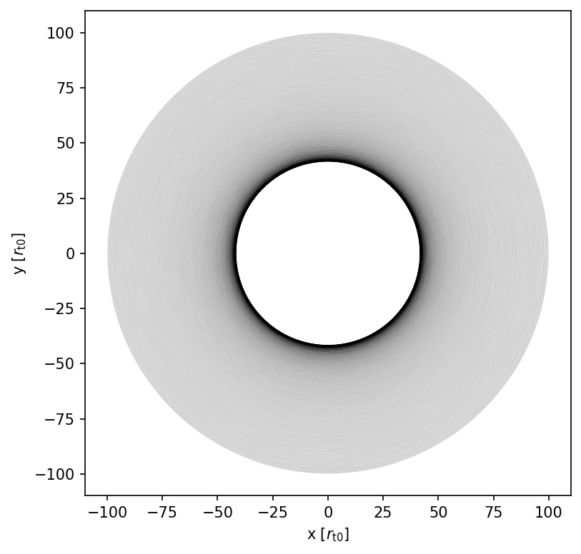
Figure 18: Orbit of a point mass under dynamical friction in the power-law potential with $\alpha=0.5$.

References

- Agarwal & Milosavljević (2011) Agarwal, M., & Milosavljević, M. 2011, ApJ, 729, 35, doi: 10.1088/0004-637X/729/1/35
- Antonini (2013) Antonini, F. 2013, ApJ, 763, 62, doi: 10.1088/0004-637X/763/1/62
- Antonini et al. (2015) Antonini, F., Barausse, E., & Silk, J. 2015, ApJ, 812, 72, doi: 10.1088/0004-637X/812/1/72
- Antonini et al. (2012) Antonini, F., Capuzzo-Dolcetta, R., Mastrobuono-Battisti, A., & Merritt, D. 2012, ApJ, 750, 111, doi: 10.1088/0004-637X/750/2/111
- Arca-Sedda & Capuzzo-Dolcetta (2014) Arca-Sedda, M., & Capuzzo-Dolcetta, R. 2014, MNRAS, 444, 3738, doi: 10.1093/mnras/stu1683
- Arca-Sedda & Capuzzo-Dolcetta (2017a) —. 2017a, MNRAS, 464, 3060, doi: 10.1093/mnras/stw2483
- Arca-Sedda & Capuzzo-Dolcetta (2017b) —. 2017b, MNRAS, 471, 478, doi: 10.1093/mnras/stx1586
- Arca-Sedda et al. (2015a) Arca-Sedda, M., Capuzzo-Dolcetta, R., Antonini, F., & Seth, A. 2015a, ApJ, 806, 220, doi: 10.1088/0004-637X/806/2/220
- Arca-Sedda et al. (2015b) —. 2015b, ApJ, 806, 220, doi: 10.1088/0004-637X/806/2/220
- Arca-Sedda et al. (2016) Arca-Sedda, M., Capuzzo-Dolcetta, R., & Spera, M. 2016, MNRAS, 456, 2457, doi: 10.1093/mnras/stv2835
- Arca-Sedda & Gualandris (2018) Arca-Sedda, M., & Gualandris, A. 2018, MNRAS, 477, 4423, doi: 10.1093/mnras/sty922
- Arca Sedda et al. (2020) Arca Sedda, M., Gualandris, A., Do, T., et al. 2020, ApJ, 901, L29, doi: 10.3847/2041-8213/abb245
- Baumgardt et al. (2019) Baumgardt, H., Hilker, M., Sollima, A., & Bellini, A. 2019, MNRAS, 482, 5138, doi: 10.1093/mnras/sty2997
- Baumgardt & Vasiliev (2021) Baumgardt, H., & Vasiliev, E. 2021, MNRAS, 505, 5957, doi: 10.1093/mnras/stab1474
- Binney & Tremaine (2008) Binney, J., & Tremaine, S. 2008, Galactic Dynamics: Second Edition
- Blumenthal et al. (1984) Blumenthal, G. R., Faber, S. M., Primack, J. R., & Rees, M. J. 1984, Nature, 311, 517, doi: 10.1038/311517a0
- Böker et al. (2002) Böker, T., Laine, S., van der Marel, R. P., et al. 2002, AJ, 123, 1389, doi: 10.1086/339025
- Bovy (2015) Bovy, J. 2015, ApJS, 216, 29, doi: 10.1088/0067-0049/216/2/29
- Capuzzo-Dolcetta (1993) Capuzzo-Dolcetta, R. 1993, ApJ, 415, 616, doi: 10.1086/173189
- Capuzzo-Dolcetta & Mastrobuono-Battisti (2009) Capuzzo-Dolcetta, R., & Mastrobuono-Battisti, A. 2009, A&A, 507, 183, doi: 10.1051/0004-6361/200912255
- Capuzzo-Dolcetta & Miocchi (2008) Capuzzo-Dolcetta, R., & Miocchi, P. 2008, MNRAS, 388, L69, doi: 10.1111/j.1745-3933.2008.00501.x
- Chandrasekhar (1943) Chandrasekhar, S. 1943, ApJ, 97, 255, doi: 10.1086/144517
- Choksi et al. (2018) Choksi, N., Gnedin, O. Y., & Li, H. 2018, MNRAS, 480, 2343, doi: 10.1093/mnras/sty1952
- Cotera et al. (1996) Cotera, A. S., Erickson, E. F., Colgan, S. W. J., et al. 1996, ApJ, 461, 750, doi: 10.1086/177099
- Do et al. (2020) Do, T., David Martinez, G., Kerzendorf, W., et al. 2020, ApJ, 901, L28, doi: 10.3847/2041-8213/abb246
- Do et al. (2009) Do, T., Ghez, A. M., Morris, M. R., et al. 2009, ApJ, 703, 1323, doi: 10.1088/0004-637X/703/2/1323
- Fahrion et al. (2020) Fahrion, K., Müller, O., Rejkuba, M., et al. 2020, A&A, 634, A53, doi: 10.1051/0004-6361/201937120
- Fall & Rees (1977) Fall, S. M., & Rees, M. J. 1977, MNRAS, 181, 37P, doi: 10.1093/mnras/181.1.37P
- Feldmeier et al. (2014) Feldmeier, A., Neumayer, N., Seth, A., et al. 2014, A&A, 570, A2, doi: 10.1051/0004-6361/201423777
- Fellhauer & Lin (2007) Fellhauer, M., & Lin, D. N. C. 2007, MNRAS, 375, 604, doi: 10.1111/j.1365-2966.2006.11308.x
- Genzel et al. (1997) Genzel, R., Eckart, A., Ott, T., & Eisenhauer, F. 1997, MNRAS, 291, 219, doi: 10.1093/mnras/291.1.219
- Ghez et al. (1998) Ghez, A. M., Klein, B. L., Morris, M., & Becklin, E. E. 1998, ApJ, 509, 678, doi: 10.1086/306528
- Ghez et al. (2003) Ghez, A. M., Duchêne, G., Matthews, K., et al. 2003, ApJ, 586, L127, doi: 10.1086/374804
- Gillessen et al. (2017) Gillessen, S., Plewa, P. M., Eisenhauer, F., et al. 2017, ApJ, 837, 30, doi: 10.3847/1538-4357/aa5c41
- Gnedin et al. (2005) Gnedin, O. Y., Gould, A., Miralda-Escudé, J., & Zentner, A. R. 2005, ApJ, 634, 344, doi: 10.1086/496958
- Gnedin et al. (2014) Gnedin, O. Y., Ostriker, J. P., & Tremaine, S. 2014, ApJ, 785, 71, doi: 10.1088/0004-637X/785/1/71
- Heggie & Hut (2003) Heggie, D., & Hut, P. 2003, The Gravitational Million-Body Problem: A Multidisciplinary Approach to Star Cluster Dynamics
- Helmi et al. (2018) Helmi, A., Babusiaux, C., Koppelman, H. H., et al. 2018, Nature, 563, 85, doi: 10.1038/s41586-018-0625-x
- Ivanov & Lin (2020) Ivanov, P. B., & Lin, D. N. C. 2020, ApJ, 904, 171, doi: 10.3847/1538-4357/abbc6f
- Iwasawa et al. (2020) Iwasawa, M., Namekata, D., Nitadori, K., et al. 2020, PASJ, 72, 13, doi: 10.1093/pasj/psz133
- Iwasawa et al. (2016) Iwasawa, M., Tanikawa, A., Hosono, N., et al. 2016, PASJ, 68, 54, doi: 10.1093/pasj/psw053
- King (1966) King, I. R. 1966, AJ, 71, 64, doi: 10.1086/109857
- Kormendy & Ho (2013) Kormendy, J., & Ho, L. C. 2013, ARA&A, 51, 511, doi: 10.1146/annurev-astro-082708-101811
- Kruijssen et al. (2015) Kruijssen, J. M. D., Dale, J. E., & Longmore, S. N. 2015, MNRAS, 447, 1059, doi: 10.1093/mnras/stu2526
- Kruijssen et al. (2014) Kruijssen, J. M. D., Longmore, S. N., Elmegreen, B. G., et al. 2014, MNRAS, 440, 3370, doi: 10.1093/mnras/stu494
- Küpper et al. (2011) Küpper, A. H. W., Maschberger, T., Kroupa, P., & Baumgardt, H. 2011, MNRAS, 417, 2300, doi: 10.1111/j.1365-2966.2011.19412.x
- Li et al. (2018) Li, H., Gnedin, O. Y., & Gnedin, N. Y. 2018, ApJ, 861, 107, doi: 10.3847/1538-4357/aac9b8
- Longmore et al. (2014) Longmore, S. N., Kruijssen, J. M. D., Bastian, N., et al. 2014, in Protostars and Planets VI, ed. H. Beuther, R. S. Klessen, C. P. Dullemond, & T. Henning, 291, doi: 10.2458/azu_uapress_9780816531240-ch013
- Loose et al. (1982) Loose, H. H., Kruegel, E., & Tutukov, A. 1982, A&A, 105, 342
- Lotz et al. (2001) Lotz, J. M., Telford, R., Ferguson, H. C., et al. 2001, ApJ, 552, 572, doi: 10.1086/320545
- Michie (1963) Michie, R. W. 1963, MNRAS, 125, 127, doi: 10.1093/mnras/125.2.127
- Misgeld & Hilker (2011) Misgeld, I., & Hilker, M. 2011, MNRAS, 414, 3699, doi: 10.1111/j.1365-2966.2011.18669.x
- Mitchell & Heggie (2007) Mitchell, D. G. M., & Heggie, D. C. 2007, MNRAS, 376, 705, doi: 10.1111/j.1365-2966.2007.11456.x
- Myeong et al. (2018) Myeong, G. C., Evans, N. W., Belokurov, V., Amorisco, N. C., & Koposov, S. E. 2018, MNRAS, 475, 1537, doi: 10.1093/mnras/stx3262
- Nagata et al. (1995) Nagata, T., Woodward, C. E., Shure, M., & Kobayashi, N. 1995, AJ, 109, 1676, doi: 10.1086/117395
- Navarro et al. (1995) Navarro, J. F., Frenk, C. S., & White, S. D. M. 1995, MNRAS, 275, 56, doi: 10.1093/mnras/275.1.56
- Neumayer et al. (2020) Neumayer, N., Seth, A., & Böker, T. 2020, A&A Rev., 28, 4, doi: 10.1007/s00159-020-00125-0
- Oh & Lin (1992) Oh, K. S., & Lin, D. N. C. 1992, ApJ, 386, 519, doi: 10.1086/171037
- Oh & Lin (2000) —. 2000, ApJ, 543, 620, doi: 10.1086/317118
- Oh et al. (1995) Oh, K. S., Lin, D. N. C., & Aarseth, S. J. 1995, ApJ, 442, 142, doi: 10.1086/175429
- Oshino et al. (2011) Oshino, S., Funato, Y., & Makino, J. 2011, PASJ, 63, 881, doi: 10.1093/pasj/63.4.881
- Perets & Mastrobuono-Battisti (2014) Perets, H. B., & Mastrobuono-Battisti, A. 2014, ApJ, 784, L44, doi: 10.1088/2041-8205/784/2/L44
- Pfeffer et al. (2018) Pfeffer, J., Kruijssen, J. M. D., Crain, R. A., & Bastian, N. 2018, MNRAS, 475, 4309, doi: 10.1093/mnras/stx3124
- Plummer (1911) Plummer, H. C. 1911, MNRAS, 71, 460, doi: 10.1093/mnras/71.5.460
- Portegies Zwart et al. (2002) Portegies Zwart, S. F., Makino, J., McMillan, S. L. W., & Hut, P. 2002, ApJ, 565, 265, doi: 10.1086/324141
- Schödel et al. (2014) Schödel, R., Feldmeier, A., Kunneriath, D., et al. 2014, A&A, 566, A47, doi: 10.1051/0004-6361/201423481
- Sersic (1968) Sersic, J. L. 1968, Atlas de Galaxias Australes
- Spitzer (1987) Spitzer, L. 1987, Dynamical evolution of globular clusters (Princeton University Press)
- Tremaine (1976) Tremaine, S. D. 1976, ApJ, 203, 345, doi: 10.1086/154085
- Tremaine et al. (1975) Tremaine, S. D., Ostriker, J. P., & Spitzer, L., J. 1975, ApJ, 196, 407, doi: 10.1086/153422
- Tsatsi et al. (2017) Tsatsi, A., Mastrobuono-Battisti, A., van de Ven, G., et al. 2017, MNRAS, 464, 3720, doi: 10.1093/mnras/stw2593
- Wang et al. (2020a) Wang, L., Iwasawa, M., Nitadori, K., & Makino, J. 2020a, MNRAS, 497, 536, doi: 10.1093/mnras/staa1915
- Wang et al. (2020b) Wang, L., Nitadori, K., & Makino, J. 2020b, MNRAS, 493, 3398, doi: 10.1093/mnras/staa480
- White & Rees (1978) White, S. D. M., & Rees, M. J. 1978, MNRAS, 183, 341, doi: 10.1093/mnras/183.3.341
- Widrow & Dubinski (2005) Widrow, L. M., & Dubinski, J. 2005, ApJ, 631, 838, doi: 10.1086/432710